The Complexity of CEO Compensation: Incentives and Learning∗

Arantxa Jarque

Richmond Fed

(PRELIMINARY AND INCOMPLETE DRAFT)

May 15, 2014

Abstract

I study what are the firm characteristics that may justify the use of options or refresher

grants in the compensation packages for CEOs as part of an optimal contract in the presence of

moral hazard. I model explicitly the determination of stock prices from the output realizations

of the firm: Symmetric learning by all players about the exogenous quality of the firm makes

stock prices sensitive to output observations. Compensation packages become an instrument

to transform this sensitivity of prices to output into the optimal sensitivity of consumption

to output that is dictated by the optimal contract. Heterogeneity in the structure of firm

uncertainty implies that some firms are able to implement the optimal contract with very simple

schemes that do not contain options, refresher grants, or perks, while others necessarily need to

use these more complex and non—transparent instruments.

Journal of Economic Literature Classification Numbers: D80, D82, D86, G30.

Key Words: mechanism design; moral hazard; CEO compensation; stock options; repricing;

refresher grants; perks; learning

1 Introduction

It is widely accepted that in order to solve the agency problem between a CEO and the owners of the

firm he works in, the compensation of the executive must be tied to the results of the firm. However,

it is less clear how the efficient provision of incentives must be implemented in practice. The recent

financial crises has revived an on—going debate about compensation practices for CEOs in US big

public firms. Although the interest in explaining the level of compensation is still present,1 there

has been a shift towards understanding the form of compensation: is the use of certain instruments,

like stock options, golden shakehands and parachutes, a sign of captured compensation boards and

misaligned incentives? In a similar spirit, concerns that certain pay practices, like the use of options,

∗I would like to thank Andy Atkeson, Marco Celentani, Huberto Ennis, Willie Fuchs, Juan Carlos Hatchondo, HugoHopenhayn, Ángel Hernando, Nobu Kiyotaki, Ned Prescott and audiences at the University of Iowa, the Feedback

group at Carlos III, and Yonsei University for valuable comments.1Academics have recently proposed explanations for the increase of the level of pay in the past decades, mainly

based on assortative matching combined with the sharp increase in the size of firms during this period (see Gabaix

and Landier (2008) and references therein).

1

may induce excessive risk taking have prompted regulatory agencies to increase their involvement in

overseeing pay practices in the banking sector. Given the state of the debate and the increased will

for intervention, a necessary first step is to enhance our understanding of the form of compensation

packages that are consistent with a correct alignment of the interests of shareholders and the CEO.

This is the objective of this paper.

Contract theory informs us about the properties of contracts that implement incentives opti-

mally (Holmstrom (1979), Grossman and Hart (1983), Wang, 1997). But such characterizations are

mainly given in a context that allows the transfers to the CEO to depend on signals of performance

(accounting measures, stock prices) in a very general way (what I will refer to as “unrestricted”

transfers). On the other hand, in real life we observe the use of a fairly limited set of compensation

instruments, like bonus programs and stock grants, which depend on accounting measures and stock

prices in specific ways. A commonly cited reason for the implementation through these type of in-

struments is their simplicity, which makes clear the ties of the compensation of the executive to the

performance of the firm. This may facilitate both the communication of objectives of stockholders

to CEOs, and the transparency of compensation practices to potential outside investors. Hence,

especially in times of heavier scrutiny of CEO pay like the ones we have seen recently, compensa-

tion boards may find it in their interest to restrict their proposals for CEO pay to commonly used

instruments that are clearly tied to firm performance measures. Another reason frequently cited for

the proliferation of stock grants is the tax advantages of compensation contingent on performance

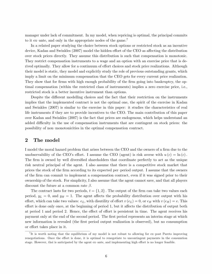
over base salaries.2 Whatever the reason, the fact is that most of the compensation given to the

CEOs of the largest public firms in the US is given in the form of salary, bonus, restricted stock

and option grants. Figure 1 illustrates this regularity for the CEOs of the largest 1,200 firms that

are listed in the S&P index.3

In spite of this evidence, a common avenue taken in the literature that studies the properties of

real life compensation instruments has been to exogenously restrict the class of instruments that

are available to the firm, and derive the optimal scheme within that class.4 The restriction on the

number and generality of instruments is necessary for practical purposes, since the complexity of

the optimization problem increases very fast with the number of instruments allowed. Although

interesting insights on the way particular instruments may work are gained with this approach, it

poses a big problem: we are restricting the firm to use an inefficient compensation scheme.

In this paper, I take a different approach: I look at the problem of implementing the optimal

contract with a rich enough set of instruments, so that the transfers given to the CEO with the

real—life instruments correspond to those derived assuming an unrestricted set of instruments. The

issue that I want to study is not whether, for an exogenously given set of compensation instruments,

2The Omnibus Budget Reconciliation Act (OBRA) resolution 162(m) of 1992 imposed a one million dollar cap

on the amount of non—performance based compensation of the top executives of the firm that qualifies for a tax

deduction. Certain restricted stock and option plans are considered performance based pay.3CEOs who owned more than 3% of the total stock of the firm at any point in the sample were considered “owners,”

i.e., not subject to a morak hazard problem, and they were dropped when constructing Figure 1.4See for example Kandan and Swinkles (2007), Clementi, Cooley and Wang (2006), Assef and Santos (2005),

Edmans and Liu (2010), or Bolton, Merah and Shapiro (2010). Alternatively, Edmans et al. (forthcoming) make

assumtions on the structure of the model that imply that very simple contracts consisting of cash and stock implement

the unrestricted optimal contract.

2

0

2,00

0

4,00

0

6,00

0

8,00

0

10,0

00

2010

US

$

1993

1994

1995

1996

1997

1998

1999

2000

2001

2002

2003

2004

2005

2006

2007

2008

2009

2010

Source: Author’s calculations using Execucomp data

Salary Bonus andIncentive Compensation

Restricted Stock Grants Option grantsOther Compensation

Figure 1: Relative importance of the different components of CEO compensation packages over

time. Column height represents average compensation.

the optimal contract is feasible, but rather what are the necessary instruments to implement it.

Just as in the data, the stylized compensation package that I consider will potentially include a

salary, a bonus program, restricted stock, options and “other compensation” (which I will refer to

as “perks”).

My framework allows me to evaluate some counterintuitive compensation practices, such as that

of issuing “refresher” grants – compensation that is set contingent on some new information on

the performance of the firm, typically to substitute option grants that have gone well out of the

money. Such practice arguably makes the compensation contract more complex, and potentially

less transparent to outside investors. In my analysis, I find that, in some instances, it is optimal

to commit to such complexity or lack of transparency: it is the least expensive way of providing

incentives for the CEO to work hard in the interest of the shareholders.

I model the moral hazard problem between the owners of the firm and the CEO as a principal

—agent problem. I propose a simple two period framework in which a risk averse CEO is asked

to exert an unobservable and costly effort in the first period only. The risk neutral owners of the

firm coordinate to act as the unique principal who designs the compensation package of the CEO.

I assume commitment to the contract for the two periods for both the CEO and the firm owners,

and I abstract from firing or quitting decisions. The effort of the CEO determines the distribution

of the results of the firm in both the first and the second period. I interpret the first period as

an interim stage at which information about performance is revealed (the company announces its

earnings in the middle of the fiscal year). New grants may be awarded to the CEO at this interim

stage (refresher grants), but no consumption takes place then; the CEO receives and consumes his

compensation in period two only, after two outcome observations are available.

Under these assumptions, if potential (risk neutral) buyers of the stock of the firm value it

according to the expected stream of future output, stock prices would not change contingent on the

value of earnings announced in the interim stage. This is because, in equilibrium, the recommended

3

level of effort is chosen. Hence, the expectations about output in the second period are independent

of the first period realization. To capture the fact that stock prices vary in reality with firm results,

I augment the model by introducing an exogenous source of uncertainty: a stochastic state that

affects the effectiveness of the effort of the CEO. This can be interpreted as the quality of the match

of the CEO and the firm, or as idiosyncratic market conditions for the firm. I assume that both

the CEO and the owners, as well as potential buyers of the stock, have a prior about this state,

which they update through Bayes’ rule when they observe a new realization of the output of the

firm. This generates contingent stock prices. As an important difference with the literature, these

assumptions imply that in my framework the distribution of stock prices contingent on effort is

endogenously generated through the learning process.

The interplay of the learning about the exogenous state and the optimal provision of incentives

has important implications for the optimal contract, which in turn influence the composition of

the compensation package. In particular, the sensitivity of compensation to price movements on

the optimal contract may decrease with the cumulative output of the firm, i.e., optimal pay may

be a concave function of cumulative output. This means that issuing options or stock grants

after a bad sequence of results (refresher grants) is needed to implement a higher sensitivity of

compensation following bad results than following good ones. In other words, the transfers implied

by real life compensation instruments are (weakly) convex in prices, by their own nature; prices

are weakly increasing and sometimes may be convex in output. In these cases, concavity of the

optimal contract can only be achieved by granting new stock or options in the interim period, even

after a bad earnings realization. What may look, to the uneducated eye, like undoing incentives,

and a sign of entrenchment, may in fact arise as part of the optimal provision of incentives.

In section 3.3 I present my conclusions about the form of real life compensation packages. I

define three types of pay schemes, according to the instruments that are included in each. My first

distinction is for schemes that include “perks,” i.e., forms of compensation that are not clearly tied

to measures of performance (for example, perquisites, pension payments, life insurance premiums,

subsidized loans, discounted share purchases or tax reimbursements). I label schemes that include

perks as “non—transparent”. In contrast, transparent schemes include only instruments that depend

on output or stock prices, i.e. they may include a bonus program and both restricted stock or

options. Within this category, I distinguish between simple schemes (including only restricted

stock issued before any realization of output is observed,) or complex (which include stock options,

or refresher grants issued contingent on the first period realization). I numerically characterize the

combinations of parameters that determine whether a firm is able to implement the optimal contract

with each type of scheme. In particular, I report the distribution of firms within the parameter

space for which a simple scheme is feasible, and those for which a non—transparent one is necessary.

I provide examples to illustrate the role of refresher grants in implementing the optimal contract

without the use of perks (i.e., with complex but transparent schemes).

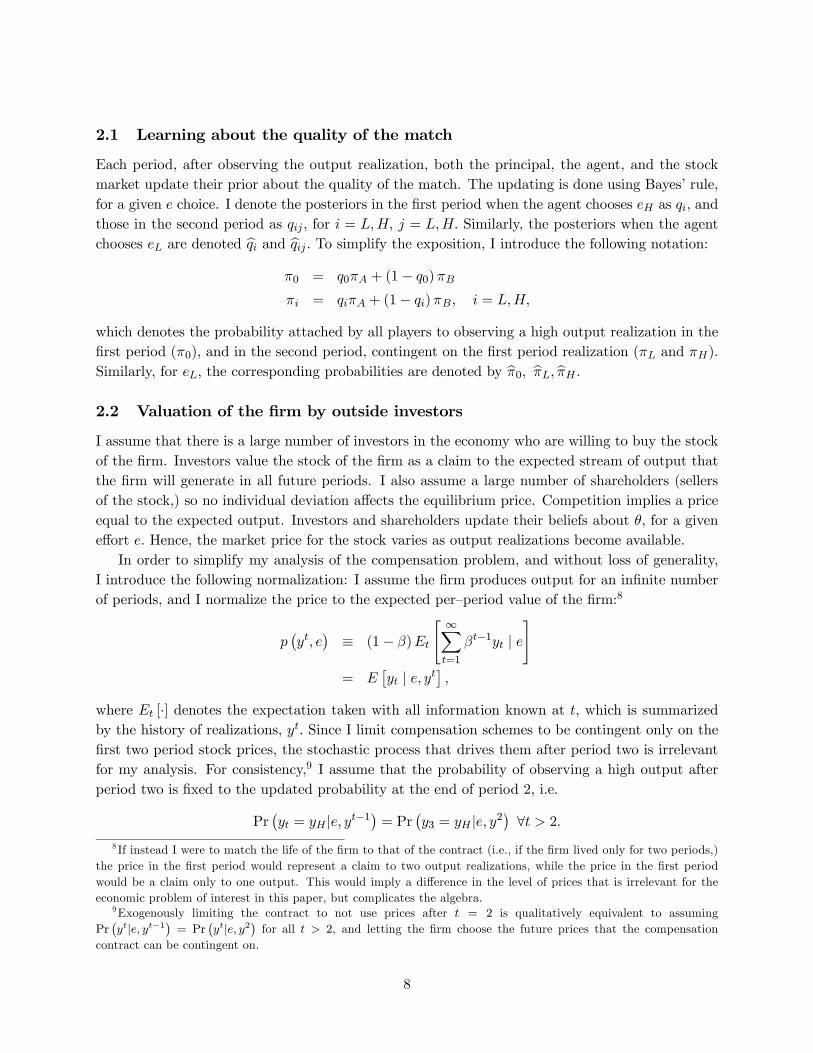
In the data publicly available about compensation practices (Execucomp), not every firm seems

to have compensation packages of the same complexity. In Fig. 2 I illustrate this fact by presenting

the percentage of firms that use stock or options in the compensation of their CEO in a given year.5

5These are all firms for which the CEO owns less than 3% of the stock, and which have a positive number

4

.75

.8.8

5.9

Ave

rage

Usa

ge o

f Gra

nts

1990 1995 2000 2005 2010Fiscal Year

Source: Author’s calculations using Execucomp data

Figure 2: Portion of firms that include stock or options in their compensation package in a given

year.

This percentage was at its lowest (77%) in 1993, and it is currently at its highest (90%). I discuss

the link of the model to the data in more detail in section 5.

1.1 Related literature

In a related theoretical paper, Acharya, John and Sundaram (2000) present a model that implies

that the practice of repricing options (i.e., changing the exercise price of options previously granted,

typically to make options that are currently out—of—the—money to be at—the—money) can be optimal

in a wide range of circumstances. The practice of repricing is, in practice, equivalent to that of

issuing refresher grants.6 Their model is also a two period problem, but they assume a risk neutral

CEO, and both output and consumption occur only at the end of the second period. In their model

there is one action every period, and the distribution of output in the second period depends on

both actions. Also, there is a signal revealed in the first period, and the agent can make his action

contingent on it. Although there is persistence through output, incentives in the second period are

independent of actions taken in the first period, and their model reduces formally to a repeated

moral hazard with consumption in the final period only. In their framework, the rigidity of options

structure that they assume implies the following inefficiency: in some branches of the second period

there are no instruments to provide incentives, and the agent does not exert (otherwise efficient)

effort. Repricing in these branches allows to implement high effort, without lowering the utility of

the agent. However, this repricing is anticipated by the agent in the first period and potentially

increases the cost of the contract. The authors show that, in many cases, the benefits of adjusting

incentives offset the cost of lack of commitment, and hence repricing is optimal.

In my model, I do not relax the assumption of commitment. Contrary to the case studied in

Acharya, John and Sundaram (2000), refresher grants or repricing do not arise to reincentivate the

(regardless of its magnitude) in either stock or option grants in the Execucomp entry for the compensation of their

CEO in a given year.6The main difference may be that options granted outside of a shareholder pre—aproved long term option plan are

not tax deductible; hence, repricing may be an attractive alternative for companies that have exhausted the options

available in their option plans.

5

manager under lack of commitment. In my model, when repricing is optimal, the principal commits

to it ex—ante, and only in the appropriate nodes of the game.7

In a related paper studying the choice between stock options or restricted stock as an incentive

device, Kadan and Swinkles (2007) model the hidden effort of the CEO as affecting the distribution

over stock prices directly. They assume this distribution is such that compensation is monotonic.

They restrict compensation instruments to a wage and an option with an exercise price that is de-

rived optimally. They allow for a continuum of effort choices and stock price realizations. Although

their model is static, they model and explicitly study the role of previous outstanding grants, which

imply a limit on the minimum compensation that the CEO gets for every current price realization.

They show that for firms with high enough probability of the firm going into bankruptcy, the op-

timal compensation (within the restricted class of instruments) implies a zero exercise price, i.e.,

restricted stock is a better incentive instrument than options.

Despite the different modelling choices and the fact that their restriction on the instruments

implies that the implemented contract is not the optimal one, the spirit of the exercise in Kadan

and Swinkles (2007) is similar to the exercise in this paper: it studies the characteristics of real

life instruments if they are to provide incentives to the CEO. The main contribution of this paper

over Kadan and Swinkles (2007) is the fact that prices are endogenous, which helps understand an

added difficulty in the use of compensation instruments that are contingent on stock prices: the

possibility of non—monotonicities in the optimal compensation contract.

2 The model

I model the moral hazard problem that arises between the CEO and the owners of a firm due to the

unobservability of the CEO’s effort. I assume the CEO (agent) is risk averse with () = ln ()

The firm is owned by well diversified shareholders that coordinate perfectly to act as the unique

risk neutral principal of the agent. I also assume that there is a competitive stock market that

prices the stock of the firm according to its expected per—period output. I assume that the owners

of the firm can commit to implement a compensation contract, even if it was signed prior to their

ownership of the stock. For simplicity, I also assume that the agent cannot save, and that all players

discount the future at a common rate .

The contract lasts for two periods, = {1 2} The output of the firm can take two values each

period, = 0 and = 1. The agent affects the probability distribution over output with his

effort, which can take two values: with disutility of effort () = 0, or with () = This

effort is done only once, at the beginning of period 1, but it affects the distribution of output both

at period 1 and period 2. Hence, the effect of effort is persistent in time. The agent receives his

payment only at the end of the second period. The first period represents an interim stage at which

new information is revealed (the first period output realization is observed), but no consumption

or effort takes place in it.

7 It is worth noting that the equilibrium of my model is not robust to allowing for ex—post Pareto improving

renegotiations. Once the effort is done, it is optimal to renegotiate to uncontingent payments in the consumtion

stage. However, thsi is anticipated by the agent ex—ante, and implementing high effort is no longer feasible.

6

The distribution over output is also affected by another parameter: a state that determines the

effectiveness of the effort of the CEO, denoted ∈ {} The true state is unknown by both theagent, the principal, and the stock market, and all players attach a prior probability of 0 to =

The probability of observing a high output contingent on an effort level and a realization of the

match is as follows, for every :

(0) (1− 0)

Pr ( = | )

b b(1)

where I assume = b = b and = b = 1 In such a firm, when effort is not effective thefirm always produces high output. This is a simplifying assumption that I will relax in section 4,

when I will consider firms for which output is always low in state ( = b = 0) and firms forwhich effort is also effective in state but it implements different probabilities than in state .

To distinguish this type of firm in matrix 1 from other types introduced later, I will refer to it as

a type H firm.

All probabilities are common knowledge. I assume that the prior over = satisfies 0 0 1

Also, higher effort () implies higher probability of observing in = that is, 1 b 0.

The timing and the stochastic structure are depicted in Fig. 1. The above assumptions on the

probabilities imply that, at time 0 all the nodes of the tree have positive probability of being

reached under both levels of effort.

Timing and probabilities of output realizations.

Matrix 1 constitutes a very stylized model of a firm’s technology. However, moral hazard

and learning are present in this technology, complicating the analysis of compensation that is the

objective of this paper.

7

2.1 Learning about the quality of the match

Each period, after observing the output realization, both the principal, the agent, and the stock

market update their prior about the quality of the match. The updating is done using Bayes’ rule,

for a given choice. I denote the posteriors in the first period when the agent chooses as and

those in the second period as for = = Similarly, the posteriors when the agent

chooses are denoted b and b To simplify the exposition, I introduce the following notation:0 = 0 + (1− 0)

= + (1− ) =

which denotes the probability attached by all players to observing a high output realization in the

first period (0), and in the second period, contingent on the first period realization ( and ).

Similarly, for , the corresponding probabilities are denoted by b0 b b 2.2 Valuation of the firm by outside investors

I assume that there is a large number of investors in the economy who are willing to buy the stock

of the firm. Investors value the stock of the firm as a claim to the expected stream of output that

the firm will generate in all future periods. I also assume a large number of shareholders (sellers

of the stock,) so no individual deviation affects the equilibrium price. Competition implies a price

equal to the expected output. Investors and shareholders update their beliefs about , for a given

effort Hence, the market price for the stock varies as output realizations become available.

In order to simplify my analysis of the compensation problem, and without loss of generality,

I introduce the following normalization: I assume the firm produces output for an infinite number

of periods, and I normalize the price to the expected per—period value of the firm:8

¡

¢ ≡ (1− )

" ∞X=1

−1 | #

= £ |

¤

where [·] denotes the expectation taken with all information known at which is summarizedby the history of realizations, Since I limit compensation schemes to be contingent only on the

first two period stock prices, the stochastic process that drives them after period two is irrelevant

for my analysis. For consistency,9 I assume that the probability of observing a high output after

period two is fixed to the updated probability at the end of period 2, i.e.

Pr¡ = | −1

¢= Pr

¡3 = | 2

¢ ∀ 28 If instead I were to match the life of the firm to that of the contract (i.e., if the firm lived only for two periods,)

the price in the first period would represent a claim to two output realizations, while the price in the first period

would be a claim only to one output. This would imply a difference in the level of prices that is irrelevant for the

economic problem of interest in this paper, but complicates the algebra.9Exogenously limiting the contract to not use prices after = 2 is qualitatively equivalent to assuming

Pr| −1 = Pr

| 2 for all 2, and letting the firm choose the future prices that the compensation

contract can be contingent on.

8

I introduce the following notation for prices. The price of the stock corresponds to the expected

value of the firm given the history of realizations, and a given effort choice:

0 ≡ (∅ ) = 0 + (1− 0) (2)

≡ ( ) = + (1− ) = (3)

≡ ( ) = + (1− ) = = (4)

under high effort, and similarly under low effort:

b0 ≡ () = 0b + (1− 0) b = b ≡ ( ) = bb + (1− b) b = b ≡ ( ) = bb + (1− b) b = =

2.3 Compensation Packages

In this section I define the compensation instruments available to the firm. I allow the compensation

package to include the following elements: an annual wage, a bonus plan, perks, and long term

performance—based plans that include both stock and option grants. With these elements I try to

capture the most important features of real—life compensation practices.10 In the year 2010, data

in Execucomp for the CEOs of the 1,500 largest public companies in the US shows that the average

pay was $4,371,060, with a minimum of $200,000 and a maximum of $25,761,432. The median pay

of the highly skewed distribution of pay was of $3,022,00.11 Of this total pay, the salary represented

an average of a 25% (or a median 19%), the bonus and incentive program represented an average

of a 25% (or a median of 23%), stock grants a 28% (median of 25%), option grants an average of

19% (median of 13%), and perks and other compensation an average of 3% (median of 1%).

I now present a brief description of each instrument and how it is captured in the model.

Base Salaries

In real life, salaries for CEOs are normally negotiated at the time of signing a contract, based

on industry benchmarks. The negotiation usually includes a pre—specified annual increase for the

duration of the contract, independently of performance.

In the model the salary is a constant payment given in period 2. I denote the salary as

Bonus plans

In real life, virtually all companies offer bonus plans paid annually based on the current year’s

performance only. They usually specify a performance target, together with a minimum and maxi-

mum limit for bonuses and the sensitivity of the bonus to the performance measure. These perfor-

mance measures consist mainly on objective measures such as net—income, revenue, pre—tax income,

10See Murphy (1999) for a detailed description of compensation instruments based on compensation surveys. See

Clementi and Cooley (2009) for a recent and careful description of the main facts related to the level and structure

of compensation of the executives of the largest public US firms in the last two decades.11This calculation excludes CEOs that at some point in their tenure with their firms owned more than 3% of the

total stock of their company; in picking this threshole I follow Clementi and Cooley (2010), who argue that such a

high ownership is not consistent with a moral hazard problem.

9

or other accounting figures. About a 25% of the total measures used in the evaluation are labeled

as “individual performance” measures, which are subjective evaluations.

In the model, I summarize these characteristics by making the bonus plan depend only on

accumulated annual output, (1 + 2) in two possible variations, as follows: = (1 2) =

min { (1 + 2)}. This mimics the structure of bonus programs in real life, were a “pool” availablefor bonuses determines a “cap” ( in this case) for annual payments.12

Perks

This instrument includes categories such as personal benefits, pension payments, perks, life

insurance premiums, subsidized loans, discounted share purchases or tax reimbursements. This

fraction of compensation is not clearly tied to any objective of performance.

In the model all these payments are simply a transfer that is contingent potentially in the whole

history of realizations. I simply refer to this category as “perks” throughout the paper, and denote

them as where = represent the first and second period output realizations.

Long term plans

In real life, compensation plans include long term payments in the form of (i) stock of the

company and (ii) options to buy stock at a pre—determined price (the “exercise” price or “strike”

price.) Both come with selling restrictions: they cannot be traded before their “vesting” time. Also,

the manager cannot take these grants with him if he leaves the company, and he is not allowed to

hedge against the risk in his compensation package.

In the model I assume that all grants vest in period 2 and they are exercised immediately by

the CEO. Consistently with real life practices, I assume an exercise price equal to the market price

of the stock at the time of granting. I denote the long—term plans as follows:

• 0: restricted stock issued in period 0

• for = : restricted stock issued in period 1 contingent on realization being observed

in period 1

• 0 : stock option grant issued at time 0 with exercise price 0

• for = : stock option grant issued at time 1 contingent on realization being observed

in period 1, with exercise price

I denote the set of compensation packages as:

P =

⎧⎪⎨⎪⎩³ 0 0 {}= {}= {}=

´ 0 0 {}= {}= {}= ∈ R+

= min { (1 + 2)}

⎫⎪⎬⎪⎭

I denote an arbitrary element of P as I assume that the principal can perfectly control the savings of the agent, and force him to sell

all stock and options when they are profitable, and consume all income generated from it. Hence,

12Results for an alteraive linear bonus program, were = (1 2) = (1 + 2) are similar and are available

upon request.

10

I introduce the following notation to denote the consumption of the agent as a function of the

compensation package: C ( ) = {}= . For any ∈ P, C ( ) takes the following form:

= + + 0 + 0 ( − 0) + + ( − ) +

= + + 0 +max {0 ( − 0)}+ +

= + + 0 +max {0 ( − 0)}+ + ( − ) + (5)

= + 0 + +

It is important to note that the function C : P→ R4+ is not injective, that is, different compensationpackages may imply the same contingent consumption vector. Using the function C we can calculatethe expected utility of the agent. For a given compensation package ∈ P and high effort, thisexpected utility is:

( ) = 20 [ ln () + (1− ) ln ()]

+2 (1− 0) [ ln () + (1− ) ln ()]−

In the same way, if the agent were to choose low effort, his expected utility would be:

( ) = 2b0 [b ln () + (1− b) ln ()]

+2 (1− b0) [b ln () + (1− b) ln ()] Finally, the cost to the principal of a contract that implements is

( ) = 20 [ + (1− )]

+2 (1− 0) [ + (1− )]

The cost ( ) is constructed in a similar manner, changing the probabilities to those corre-

sponding to low effort.

2.4 Incentive problem

With the compensation packages and the consumption function in hand, we are now ready to write

the optimization problem of the principal. I assume throughout that parameters are such that it

is always profitable to implement Hence, the optimal compensation package ∗ is the solution

to the following cost minimization problem, where represents the outside utility the agent would

obtain if he were not to participate in the contract:

( ) = min∈P ( ) (P1)

≤ ( ) (PC)

( ) ≥ ( ) (IC)

11

0 0 ≥ 0 (NNC)

Problem P1 is difficult to solve in general, due to the large amount of non negativity constraints in

(NNC). I propose, instead, to solve a simplified problem in which the principal chooses directly a

tuple = {}= of transfers contingent on the history of output realizations, as follows:

() = min ( ) (PS)

≤ ( ) (PC’)

( ) ≥ ( ) (IC’)

≥ 0 (NNC’)

I denote the solution to PS as ∗ ≡n∗o=

The standard arguments valid for a static moral

hazard problem (see Grossman and Hart, 1983) justify that both the PC and the IC constraints

bind in the optimum. Note that the agent has logarithmic utility, so the non—negativity constraints

(which are now in terms of consumption levels) will never bind. Also, with a simple change of

choice variables to utility levels, the objective function is linear and the constraint set is compact

and convex, so the solution to PS exists and is unique.

Lemma 1 Any solution ∗ to problem P1 implements the same consumption for the agent as the

solution ∗ to the simplified problem PS.

It is easy to see that the set of available compensation instruments P is rich enough to implementany (positive) transfer scheme contingent on the history of output realizations, i.e., any value for

the tuple {}= . This result implies that I can study the problem of choosing the instrumentsseparately from the determination of contingent consumption in the optimal contract. However,

since the function C ( ) is not invertible there might be several compensation packages that solveproblem 1 and satisfy C ( ) = ∗

3 Equilibrium

Recall from section 2.2 that individual deviations of the shareholders and the investors do not affect

the stock prices in the equilibrium of the stock market. This implies that there are only two pricing

rules that may appear in any equilibrium: one for any contract that implements and one for

any contract that implements . By changing his effort, the CEO can only affect the probability

distribution over prices, but not the prices themselves.

An equilibrium of the above game between the principal, the agent and the stock market is

defined next.

Definition A Perfect Bayesian Equilibrium of this game in which effort is implemented consists

of a compensation contract ∗, and stock prices such that

12

) C ( ∗) = ∗ where ∗ = argmin{} ( ) and

) The utility of the agent choosing is higher than if choosing and is as large as his outside

utility

) Market prices and the beliefs of the stockmarket participants about are consistent with the

agent choosing as defined by 0 in Equations (2) -(4)

) Beliefs about are updated according to Bayes’ rule.

Since the probability of observing any history is positive under the equilibrium level of effort,

Bayesian updating provides consistent beliefs, and no refinement is necessary.

In the next subsections I describe the properties of the equilibrium.

3.1 Equilibrium Stock prices

All stock traders anticipate that, in equilibrium, the agent chooses the recommended level of effort,

Hence, they update their beliefs using the probabilities in the above matrix corresponding to

The equilibrium price of the stock corresponds to the expected value of the firm given the

history of realizations, given by and in Equations (2) -(4). For the rest of the analysis in the

paper, it will be useful to keep in mind the following property of stock prices:

Lemma 2 Stock prices are monotonic in the period’s output: ≤ and ≤ = ≤

In particular, for any histories containing at least one , the updated believes put probability

one on = , i.e., we have that H = 1 if or equals . If the observed history does not containany , instead, = has still positive probability. This is the case for histories and ( )

That is,

= 0

0 + 1− 0

= 02

02 + 1− 0

= = = 1

A direct implication of this learning is that the stock prices take the simple form:

0 = 0 + 1− 0 (6)

= + 1−

= + 1−

= = =

13

3.2 Equilibrium Consumption

Problem PS is a particular example of a static moral hazard problem, with i.i.d. output and

exogenous uncertainty about the probability distribution implemented by each effort level. The

characterization of the optimal contract with unrestricted instruments follows easily from the stan-

dard first order conditions of problemPS. Define the likelihood ratio (LR) of a history of realizations

as the ratio of the expected probabilities of that history under low and high effort:

=b00

b

=0b2 + 1− 0

02 + 1− 0

=b00

1− b1−

=(1− b) b(1− )

=1− b01− 0

b

=(1− b) b(1− )

=1− b01− 0

1− b1−

=(1− b)2(1− )2

(7)

Proposition 1 Consumption levels in the optimal contract ∗ are ranked by likelihood ratios:

∗ ∗ ⇔ for ∈ {}

Moreover, consumption is linear in the LR:

∗ = + (1− ) (8)

where is the multiplier of the constraint PC and that of the constraint IC.

It is worth noting that, if were for sure, the above characterization would always imply the

same ranking for consumptions for all combinations of parameters, as the next proposition states.

Define ∆ ≡ ∗ − ∗ and ∆ ≡ ∗ − ∗

Proposition 2 In the absence of learning about (certainty case with = ) the optimal con-

sumption is monotonic in output and it satisfies:

0 ∆ ∆

With uncertainty about , however, the posterior evolves differently under than changing

the weight of each probability in the numerator and denominator of the LR. As stated in the

next proposition, this can create non—monotonicities. The intuition for the existence of non—

monotonicities in the optimal contract is that learning shifts the weights given to certain histories

in the provision of incentives, with respect to the benchmark case characterized in Prop. 2. Since

the value of is not controllable by the agent, the principal would like to insure him against this

risk. However, under such a contract, the agent would shirk and blame poor performance on a bad

realization of . The optimal contract, hence, demands exposing the agent to some -related risk.

This, in turn, may lead to non—monotonicities in consumption, since the principal evaluates the

14

relative likelihood of effort and learns about the realization of at the same time. For example, a

high outcome following a low one may increase the likelihood that the first observed (low) output

was the result of low effort; hence, a high second period outcome is “bad news” for the agent. In

other words, the weights given to each ’s probability distribution (i.e., the posteriors,) are different

for high and low efforts, so the ordering of each ’s probabilities is not preserved in the probability

unconditional on .

As pointed out previously, for our benchmark firm we have = = = 1 This may

mean that, when the first period output has been the agent’s wage may be higher if we observe

in the second period than if we observe This is because observing in the second period

reveals that = In state the first period observation makes the history’s likelihood ratio

be much lower (it is a much less likely history under low effort than it would be if = ).

We can use the likelihood ratios in 7 to establish the following properties of consumption in the

optimal contract:

Proposition 3 When the firm is of type H, consumption spread always satisfies ∆ ∆ Also,

non-monotonicities never arise in the lower consumption, i.e., ∆ 0 always. Moreover, we have

(i) whenever + b 1 for all 0 ∈ (0 1) 0 ∆

(ii) whenever + b 1

for 0 ∈ (0 ∗) 0 ∆

for 0 ∈ (∗ 1) ∆ 0

where ∗ = 1−−+

The fact that non-monotonicities only arise in ∆ and only when + b 1 is related to the

interaction of the informativeness of the signal ( ) (or, equivalently, ( )) and the learning

about the true state. On one hand, + b 1 implies that is less than one, and hence the

optimal contract seeks to reward the agent when observing as well as when observing

Punishments are reserved for However, observing reveals perfectly that the true state is

making a more informative signal about effort than if there were still positive probability

on state (which is the case when we observe ) This tends to make large, but not

making ∆ large and ∆ small. For high enough 0 the relative informativeness of and

may be reversed and we may get ∆ 0

We conclude this section summarizing the properties of the optimal contract derived from the

above propositions:

1. Contingent consumption is ranked by the LR of output realization histories.

2. Since = we have =

3. Consumption in the optimal contract may be non monotonic in output in the second period:

4. We have ∆ ∆ always.

15

3.3 Equilibrium compensation packages

The analysis of the properties of equilibrium consumption in the previous section was based on

the solution to problem PS, with contingent consumption transfers ∗ In this section, we use theC (∗) mapping, together with the properties of ∗ to analyze the characteristics of the solutionto the original problem P1 in terms of compensation packages in P.

The first thing to note is that given the richness of the elements of P, the optimal contract ∗

characterized in section 3.2 is always feasible in a trivial way: because of the availability of perk pay-

ments, the firm can simply set = ∗ for all pairs. However, there may be other combinationsof compensation instruments that implement a given optimal contract. To solve the indeterminacy

of the compensation package, I assume that the principal, when presented with several choices

to implement a given contingent consumption scheme, chooses the simplest possible. That is, I

study the properties of the compensation packages that implement the optimal contract ∗ withthe simplest possible compensation package, and the most transparent one. I define simplicity and

transparency next.

Consider the following strict subsets of P :

S = { ∈ P such that 0 = 0 ∀ } C = { ∈ P\S such that = 0 ∀ }

Definition A compensation package is classified as:

• Transparent if it does not include any perks, i.e. ∈ C ∪ S

— Simple: if it is transparent and it includes only a wage, bonus scheme and restricted

stock granted at time 0, i.e., ∈ S— Complex: if it is transparent and it includes at least one option grant or a refresher

stock grant, but no perks, i.e., ∈ C

• Non-transparent: if it includes at least one contingent perk payment, which dependenceon performance is not transparent to an outsider, i.e., ∈ C ∪ S

In the rest of the paper, I ask the following questions: What types of firms are not able to use

a transparent scheme, and which are? Which can do with just a simple scheme?

To answer these questions, I use the following strategy. First, I spell out C ( ) under therestrictions implied by a simple and a complex scheme, with each of the two types of bonus programs

that I consider. Then, I analyze the system of equations resulting from equating C ( ) = ∗

Definition Consider a firm defined by a probability structure of the form of matrix (1). A compen-

sation scheme is feasible if, for the ∗ corresponding to the parameter values that describethe firm, the system of equations resulting from equating C ( ) = ∗ has a solution and thissolution satisfies the non—negativity constraint in (NNC).

16

Although restricting to schemes in the subsets S and C simplify the system C ( ) = ∗, it isdifficult to characterize the solution (or even to check constraint NNC) in general. In what follows,

I present a series of results that constitute a partial characterization of the choice of compensation

packages between simple, complex or non—transparent. I complement my analysis with a complete

numerical characterization of this choice.

A simple benchmark: no learning

As a preview of the method that I use to establish feasibility of the different compensation

packages, and for benchmark purposes, I analyze first the no—learning case discussed in Prop. 2).

Proposition 4 If there is no learning, compensation packages must be non—transparent.

The proof is simple so I include it in the text. It is easy to see that no in S or C is feasibleby looking at the system ∗ = C ( ) given that all prices are equal to For a linear bonus,

∗ = + 0

∗ = + + 0

∗ = + 2+ 0

It is useful to write these equations as a function of the consumptions spreads:

∗ = + 0

∆ =

∆ =

Any solution implies = ∆ but also ∆ = ∆ which is never true because ∆ ∆ by Prop.

2. If a capped bonus were used instead, the system would read:

∗ = + 0

∆ =

∆ = 0

In this case, we would need ∆ = 0 which, again by Prop. 2, is not possible.

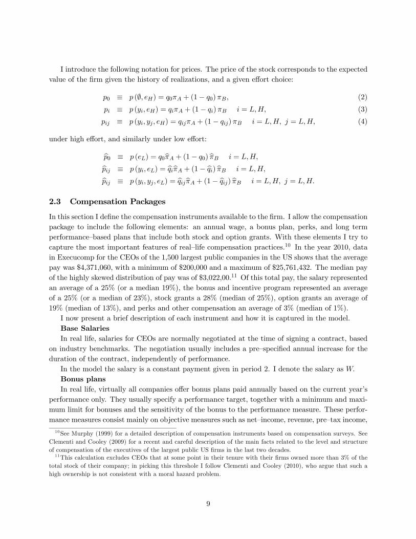
Figure 3 illustrates an example without learning in which 0 = 1 = 08 and b = 04 It iseasy to see graphically that having only one price implies that any difference between ∗

∗

and ∗ needs to be implemented with the bonus program exclusively, and this is not feasible if it

takes one of the standard forms (linear or capped).

3.3.1 Non—transparent schemes

By simple inspection of the system ∗ = C ( ), we can see that payments to the agent are necessarilymonotonic in output, and hence monotonic in prices, since prices are themselves monotonic in

output. As the following proposition describes, monotonicity of the optimal consumption is both a

necessary and a sufficient condition for a complex scheme to be feasible

17

0 p

c_LL

c_LH

c_HH

Consumption and prices for each history

p(yt)

c(yt )

Figure 3:

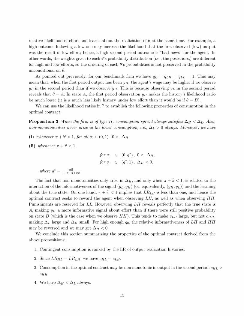
Proposition 5 For a firm of type H, compensation schemes must be non—transparent if and onlyif non—monotonicities arise (∆ 0).

Figure 4 presents graphically the analytical characterization in Prop. 3 of the parameters that

imply a non—monotonicity. For this, we assume that, for each feasible combination of and bthere is a mass one of firms whose prior 0 is distributed uniformly between 0 and 1. The vertical

axis, then, represents the proportion of firms for which non—monotonicity is present in the optimal

contract. We see that, when is high enough, or the difference −b is large enough (both cases thatlead to +b 1), consumption is monotonic. For the combinations that imply non—monotonicities,

with + b 1 it is the firms with the largest priors, 0 ∗ as defined in Prop. 3, that need touse non—transparent schemes.

3.3.2 Simple schemes

In this section, I provide necessary and sufficient conditions for the feasibility of a simple com-

pensation package in the presence of learning. One caveat is that the conditions will not be, in

general, in terms of the primitive parameters of the firm. I complement the analytical derivations

with numerical characterizations.13

Proposition 6 A simple scheme is feasible if and only if

a) ∗ (1−)∆ , and

b) ∆ 0 or, equivalently, 0 ∗ = 1−−+ (see Prop. 3)

The conditions in this proposition are restrictions that the structure of compensation instru-

ments imposes on the sensitivity of the consumption of the agent to changes in stock prices. This

sensitivity is sort of a reduced form for the composition of the sensitivity of consumption to signals

(i.e., output realizations), which is dictated by the likelihood ratios, and the sensitivity of prices to

13The proof of Proposition 6 follows from the proof of a more general statement, Prop. 15, included in Appendix

2.

18

0.1

0.2

0.3

0.4

0.5

0.6

0.7

0.8 0.2

0.3

0.4

0.5

0.6

0.7

0.8

0.9

0

0.2

0.4

0.6

0.8

1

pi

Non−Transparent scheme for B firm (dH < 0)

pihat

% o

f q0

Figure 4: Type H firm. Probability that non—monotonicities arise and a Non-transparent scheme

is necessary.

signals, which is in turn dictated by the pricing rule of outside investors. The proposition shows

that a limited set of compensation instruments like S puts severe restrictions on the relationship ofthese two sensitivities.

In particular, the proposition can be otherwise stated as a simple scheme being feasible whenever

the following solution satisfies the non—negativity constraint for the three instruments:

= ∗ − ∆

(1− )¡1− H

¢ = ∆

0 =∆

(1− )¡1− H

¢ For a firm of type H any number of low outputs is perfectly informative about the state. Hence,there is no variation in prices in the lower range, implying that the spread − needs to

be implemented with the bonus payout: = ∆ Setting the bonus to satisfy this constraint is

always feasible, since ∆ 0 always for a firm of type H. Since the bonus is capped, the spread − needs to be implemented with restricted stock:

∆ = 0 ( − )

This is feasible whenever the optimal consumption is monotonic, so that we have∆ 0 (condition

) in the above corollary). For a firm of type H high output levels are purely out of luck if weare in state which means that no incentives are needed in the upper range of output. Hence,

19

0.1

0.2

0.3

0.4

0.5

0.6

0.7

0.8 0.2

0.3

0.4

0.5

0.6

0.7

0.8

0.90

0.1

0.2

0.3

0.4

0.5

0.6

0.7

0.8

0.9

1

pi

Feasibility of simple scheme for B firm

pihat

% o

f q0

Figure 5: Fraction of firms for which a simple scheme is feasible (type H firm).

only for high enough prior that we are in state incentives are high powered enough to make ∆

positive. Finally, the level of needs to be implementable, given the restricted stock 0 with a

positive wage:

= − 0

This is feasible whenever condition ) in the corollary is satisfied. If the 0 needed to implement

∆ or are too high, a simple scheme is not feasible.

Unfortunately, condition ) depends, also for this type of firm, in a non trivial way on the

primitives of the model (through ∗) Although it is not possible to provide an analytical charac-terization of the combination of primitives for which it is satisfied, it is easy to check it numerically.

Fig. 5 plots the probability that both condition ) and ) are satisfied, and hence a simple scheme

is feasible for a firm of type H. The values that make it most likely are combinations of high valuesof with intermediate values of Whenever takes values above 0.4, no combination of and 0

makes a simple scheme feasible.

3.3.3 Complex schemes

Proposition 7 A complex scheme is feasible (with a capped bonus) if and only if ∆ 0, i.e., if

0 ∗ = 1−−+

Hence, condition b) in Prop. 6 is both necessary and sufficient for a complex scheme to be

feasible. The proof of this proposition (see Appendix 2) presents the expressions for the solutions

to the optimal packages. The system is undetermined, i.e., if it has a solution it has an infinite

number of them. However, only solutions that satisfy the non—negativity constraints on all the

20

instruments constitute feasible complex schemes. In the proof of the sufficiency it is shown that

whenever ∆ 0 we can construct a feasible scheme that uses only a limited set of instruments:

=

= ∆

=∆

− 0 = 0 = = = = 0

Hence, a refresher stock grant given to the agent after observing a high output in the first period

is instrumental in implementing the optimal scheme. Given that there is no variation in prices

following a low realization in the first period, the bonus needs to be used to implement ∆ Since

∆ ∆ the bonus needs to be capped. Hence, an instrument that will only pay off in the HH

history is needed - an option granted when market price is equal to

Given that condition b) in Prop. 6 is both necessary and sufficient for a complex scheme to

be feasible, a natural question is whether there is a non—trivial role for complex instruments. Can

they help in the implementation of the optimal contract when a simple scheme is not feasible?

The answer to these questions is positive. The next proposition illustrates that there is a role for

refresher stock grants and option grants.

Proposition 8 There is a non empty set of firms (parameter values) for which a simple scheme

is not feasible but a complex one is.

Figure 6 presents graphically the combinations of 0 and for which simple scheme is not

feasible but a complex one is (condition a) in Prop. 6 is violated but condition b) is satisfied).

4 Generalization of the model

A more general firm description than the one I have been using as the leading example (the type Hfirm) would be one as in matrix 1, where output in state is not only stochastic but it also depends

on the effort choice of the agent. When considering this general case, I assume that 6= b for atleast one and the prior over = satisfies 0 0 1 Also, higher effort () implies higher

probability of observing (for any quality of the firm): ≥ b and ≥ b with at least onebeing a strict inequality. For a firm of this generality, moral hazard and learning interact in more

complicated ways; however, the intuition behind the properties of optimal consumption will rely

on the same forces highlighted earlier for a type H firm.

It is my goal in this section to illustrate the usefulness of the results related to a firm of type

H to understand what drives the feasibility of compensation schemes for a firm of the general case.

For that purpose, I now introduce a second special type firm. Let a firm of type L be described,for all by:

L (0) (1− 0)

Pr ( = | )

0

b 0

(9)

21

0.10.2

0.30.4

0.50.6

0.70.8

0.90.1

0.2

0.3

0.4

0.5

0.6

0.7

0.8

0.9

0

0.2

0.4

0.6

0.8

1

pi

Probability that complex scheme is feasible but simple scheme is not, type H firm

pihat

% o

f q0

Figure 6: Proportion of firms for which a simple scheme is not feasible but a complex one is (type

H firm).

In such a firm, when effort is not effective the firm always produces low output. In contrast, we

may refer to the firm we have analyzed in the core of the paper as a type H firm, since output is

always high in the state when effort is not effective.

Firms of typeH and L represent particular examples of technologies that we may identify in reallife. For example, we may think of H firms as mature, successful ones in which only the possibility

of a bad match triggers bad realizations. Type L firms, instead, may be younger, struggling firmsfor which only a good match paired with high effort may improve outcomes. Other interpretations

relate to the dependence of the firm’s results on exogenous factors, such as uncertain new regulations

or R&D developments.

Moreover, these two types of firms may be valuable in understanding the determinants of

compensation packages in firms of a more general type, as described next. To see this, consider

the following case: When the quality of the firm is a high output is realized with probability

regardless of the effort choice of the agent. Learning interacts with the moral hazard problem in

this setting in a more general way than in the type H and L firms, since a high output observationis more or less informative about the moral hazard problem depending on the particular value of

. It is easy to see that, for 1 that satisfies

= 1 + (1− 0 − 1) 0 = 1

we can think of this case as a firm whose effort effectiveness varies across three states of the world:

in it is effective, in 1 output is always high, and in 2 output is always low. That is, whenever

effort is not effective, output is high with probability 1, and low with probability 1− 0 − 1.

22

0.1

0.2

0.3

0.4

0.5

0.6

0.7

0.8 0.2

0.3

0.4

0.5

0.6

0.7

0.8

0.9

0

0.2

0.4

0.6

0.8

1

pi

Non−Transparent scheme for G firm (dH − dL > 0)

pihat

% o

f q0

Figure 7: Type L firm. Probability that ∆ −∆ 0 is satisfied and a Non-transparent scheme

is necessary.

Next, I summarize the analyses of a type L firm, the details of which are included in the

appendix.

4.1 Firm of type LDerivations for the results regarding type L firms, which parallel those of a typeH firm, are includedin the appendix. Here, I present the discussion of the results, and compare them to those of a type

H firm.

4.1.1 Non—transparent schemes

For a firm of type L non—monotonicities never arise following a high realization in the first period(∆ 0 always), but we may have ∆ ∆ and non—monotonicities following a low realization

in the first period (∆ 0)

Proposition 9 For a firm of type L, compensation schemes must be non—transparent if and onlyif ∆ ∆ .

Prop. 13 in Appendix 2 characterizes formally the set of parameters for which ∆ ∆ , and

hence a non—transparent scheme is necessary for a type L firm. Figure 7 presents this characteri-zation graphically.

23

0 p_LL p_LH=p_HH

c_LL

c_LH

c_HHConsumption and prices for each history

p(yt)

c(yt )

Figure 8: Mapping of consumption to prices for the L firm in Example 1 (see matrix ??).

4.1.2 Simple schemes

Figure 8 represents an example of the mapping between consumption and stock prices for a firm of

type L The infeasibility of a capped bonus is straight forward: because for an L firm, =

or = 0 we have that, under a capped bonus, ∆ needs to be zero. This means that the only

case in which a simple scheme could implement the optimal scheme is one in which ∗ = ∗ But

this is never the case for the non-trivial parametrization that we study, with 6= b and 0 ∈ (0 1).On the other hand, a linear bonus, defined as = (1 + 2) may be feasible (see Corollary 2

in the Appendix for details). Conditions ) and ) in Corollary 2 summarize when the following

solution satisfies the non—negativity constraint for the three instruments:

= ∗ − ∆ −∆¡1− L

¢ = ∆

0 =∆ −∆¡1− L

¢

The form of this solution is intuitive. For a firm of type L any number of high output realizationsis perfectly informative about the state, so there is no variation in the upper range of prices (see

Figure 8). This means that the spread − needs to be implemented through a bonus payout: = ∆ Given the linear bonus program, this is not a problem as long as ∆ ≥ ∆ If this is the

case, the quantity of restricted stock is determined to satisfy

∆ − = 0 ( − )

It is the case that ∆ ≥ ∆ whenever incentives need to be more high powered in the low range of

outcomes; since an L firm is more likely to get low output levels out of luck (when the true state is

,) incentives are high powered in the low range of outcomes only for high enough prior that the

state is Finally, it must be the case that the implied wage given 0 is positive (condition ) in

Corollary 2):

= − 0

If this condition is not met, a simple scheme is not feasible.

24

0 p_LL p_LH=p_HH

c_LL

c_LH

c_HHConsumption and compensation instruments for s0 = 0

p(yt)

c(yt )

Figure 9: A simple compensation package is feasible for the firm in Example 1. The wage is

where the blue line intersects the vertical axis. The blue line represents the sum of plus the

value of the 0 stock grants as a function of the stock price. The green line represents the value of

the wage, plus the 0 stock plus the payoff of the bonus scheme if only one is realized (). The

red curve represents the value of the wage, plus that of 0 plus the payoff of the bonus scheme if

two are realized (2).

Example 1 The following parameters describe an example of a firm of type L for which a simplelinear bonus is feasible: = 04 = 03 0 = 8 The mapping between optimal consumption

and prices is depicted in Figure 8. The the optimal simple package is superposed in Figure

9: the wage is slightly bellow so that 0 stock grants (the value of which, as a function

of the stock price, is plotted in blue) satisfy + 0 = The green line represents the

value of the 0 stock plus the payoff of the bonus scheme if only one is realized, , and the

red curve that of 0 plus the payoff of the bonus scheme if two are realized, 2.

Fig. 10 presents the feasibility of a simple scheme for a firm of type L. Assuming a uniformdistribution of 0 in the population, the probability that conditions ) and ) in Corollary 2 are

satisfied for a firm of type L is depicted. The height of the mountain can be interpreted as theprobability that the relationship between 0 and b characterized in Prop. 13 is met, for a firmof randomly draw 0.

14 The highest probability is for high values of combined with low values of

Small differences − are only sustainable for values between 0.3 and 0.4; for values of close

to 0.2 or close to 0.9, even for differences of − = 02 a simple scheme is not feasible for any 0.

4.1.3 Complex schemes

The analysis parallels that of type H firms.

Proposition 10 A complex scheme is feasible (with a capped bonus) if and only if ∆ ∆

14Note that when I present this type of graphics, only the feasible combinations of probabilities are plotted (i.e.,

pairs that satisfy ).

25

0.10.2

0.30.4

0.50.6

0.70.8 0.2

0.30.4

0.50.6

0.70.8

0.90

0.1

0.2

0.3

0.4

0.5

0.6

0.7

0.8

0.9

1

pi

Feasibility of simple scheme for type L firm (15 q0 values between .25 and .9)

pihat

% q

0

Figure 10: Feasibility of a simple scheme for a type L firm (with a linear bonus).

Complex schemes that are feasible when ∆ ∆ also take a very simple form:

=

= ∆

=∆ −∆

=∆ −∆

− 0 = 0 = = = 0

where the bonus is linear in this case.

Again, we may ask whether there is a non—trivial role for complex schemes; the answer is positive

as well for type L firms.

Proposition 11 There is a non empty set of firms (parameter values) for which a simple scheme

is not feasible but a complex one is.

Figure presents a numerical characterization of the set of parameters. Here I provide an example

of the role of refresher grants in implementing the optimal contract without using non—transparent

schemes, for a firm of type L.

Example 2 The following parameters describe an example of a firm of type L for which a simplelinear bonus is not feasible: = 04 = 03 0 = 9 In this example, condition ) is violated.

In figure 12 we see graphically that a simple implementation with a linear bonus would imply

26

0.1

0.2

0.3

0.4

0.5

0.6

0.7

0.8

0.90.1

0.20.3

0.40.5

0.60.7

0.80.9

0

0.1

0.2

0.3

0.4

0.5

0.6

0.7

0.8

0.9

1

pi

Probability that a complex scheme is feasible but a simple scheme is not, type L firm

pihat

% o

f q0

Figure 11: Proportion of firms for whic a simple scheme is not feasible but a complex one is (type

L firm).

0 p_LL p_LH=p_HH

c_LL

c_LH

c_HHConsumption and compensation instruments for s0 = 0

p(yt)

c(yt )

Figure 12: For the firm of type L in Example 2, described by matrix (??), condition ) is violated

and hence a simple scheme is not feasible.

27

0However, I now show that the optimal contract can in this case be implemented with

a complex scheme consisting of a linear bonus, 0 0 0 and 0 With ∈ C, andunder the parametrization of example 2, we have:

= + 2+ 0 +

= + + 0 +

= + + 0 + ( − )

= + 0

The solution is:

= −

1− (∆ −∆) +

= ∆

0 =∆ −∆

(1− )−

=

We draw the following conclusions from comparing our benchmark firm to a type L firm. Fora firm that tends to be more successful when effort is very effective (type L), prices are not assensitive to output realizations as the optimal incentives; this implies that, although the firm may

be able to use a simple scheme consisting only of a wage, restricted stock and a bonus program, the

bonus should be linear in output. Instead, for a firm that tends to be more successful for exogenous

reasons than for the effect of effort (type H), prices are not as sensitive to output realizations whenthey are low as the optimal incentives should be; this implies that when a simple compensation

scheme is used, the bonus program should be capped.

5 Discussion of testable implications

What do we know about the real life relationship between firm characteristics and the use of

different compensation instruments? Here I present some regularities that emerge from my analysis

of Execucomp data on CEO compensation, and relate them to the conclusions of my model.

It is a difficult task to identify “refresher” grants in the data. Typically, however, new grants

are awarded before the selling restrictions on previous grants has expired. Hence, I interpret all

restricted stock grants as refresher grants ( and in my model). Based on the usage data

presented in figure 2, I construct a classification of “users” and “non-users” that is based on

observing repeated option or stock grants by the same firm over time.15 Because size and industry

have been shown to be important determinants of pay level (see Murphy (1999), Gabaix and

15All firms are in the sample for at least 6 years. I define “users" as firms that have granted in at least 70% of the

total years that they are in the sample. I define “non-users” as firms that have granted 4 years or less, or in less than

50% of the years they are in the sample. Out of 1,457 firms, this generates 145 non—users, 1,186 users, and 126 firms

that cannot be classified (I drop them from the analisys). There are 6 firms in the sample that never use any grant,

and 116 that use them in every one of the 18 years in the sample.

28

51015202530

(mea

n) e

mpl

1990 1995 2000 2005 2010Fiscal Year

Users Non−Users

02

46

0 20 40 60 0 20 40 60

Non−Users Users

Den

sity

Tenure of the executive in yearsGraphs by users

2000

4000

6000

800010

00012

000

(mea

n) s

ales

_rea

l

1990 1995 2000 2005 2010Fiscal Year

Users Non−Users

0.2

.4.6

Min.

/Man

.FIR

E

Utilitie

sOth

er

Min.

/Man

.FIR

E

Utilitie

sOth

er

Non−Users Users

Den

sity

sic4Graphs by users

Source: Author’s calculations using Execucomp data

Figure 13: Differences between “users" and “non-users" of grants, in terms of (from left to right,

top to bottom): the average number of employees of the firms, the average tenure of the CEOs, the

average value of annual sales, and the distribution of the firms across industries.

Landier (2008), and Clementi and Cooley, 2010), I also consider differences across the two groups

for measures of size and SIC industry classification.

In Fig. 13 we can see that user firms are larger in terms of employees, and they are larger also

in terms of their volume of annual sales. However, we do not have a good a priory explanation of

why larger firms should be more likely to be users of grants in compensation. On the other hand,

users are more likely to be Mining and Manufacturing firms, which are sectors that tend to pay less

than sectors like Finance, Insurance and Real Estate (FIRE) (Clementi and Cooley, 2010). User

firms also tend to employ CEOs for a longer tenure, as evidenced by the histogram of the average

tenure at the firm level in the upper right hand side corner of Fig. 13. The empirical evidence

about the potential complementarity of career concerns and explicit incentives is mixed; also, one

may consider the possibility that firms that have a reputation of longer tenures can expose the

CEO to higher risk through his compensation package to compensate for the added job security.

Hence, the effect on the decision to use grants is not obvious.

SIC classification % of users Total firms Users Non—Users

Utilities 0.80 163 131 32

Other 0.88 313 275 38

FIRE 0.91 197 180 17

Mining and Manufacturing 0.94 639 600 39

29

Table 1: Proportion of Users and Non-Users in a four group classification of industries.

In table 1 I report the proportion of firms that qualify as “users” in four different groups of firms,

according to their SIC industry classification. Firms in “Utilities”, which includes Transportation,

Communications, Electric, Gas, And Sanitary Services, are the ones who rely less often on grants.

On the other hand, firms in Finance, Insurance and Real Estate (FIRE) are not the ones that use

them more intensely, as one may conjecture: firms in Manufacturing and in Mining use them more

broadly, at a 94% rate.

Small firms seems to be less likely to use grants, i.e. they seem more able to use simple schemes.

Because size (employee numbers and sales volume) is correlated with the age of the firm and its

reputation, it may be important in determining the effectiveness of the actions of its CEO (whether

the firm is of type L or H, and what is the value of ) The tenure of the CEO may be related tothe level of uncertainty that the firm faces (the prior in the model).

The empirical literature in Finance has also provided some interesting –although scarce–

evidence about complex or non—transparent compensation practices: refresher grants, and repricing.

Hall and Knox (2004) find evidence that refresher grants are often used by firms both following

a stock price decline and following a stock price increase. They interpret refresher grants as a

mechanism to restore incentives for the CEO whenever the sensitivity of his compensation to stock

price movements decreases. This makes refresher grants following a stock price increase puzzling,

since stock price increases tend to increase the sensitivity of pay to firm performance. My model

provides a rational for new grants contingent on both good and bad firm performance.

A related compensation practice, option “repricing,” consists in lowering the exercise price of

options that have gone out—of—the—money (i.e., their exercise price is well above the current stock

price in the market.) This can be thought of as a substitute for refresher grants, but with potentially

different tax implications. Although this practice is fairly uncommon (Brenner, Sundaram and

Yermak (2000), report that 1.3% of the top five officers in a sample of 1500 firms between 1992

and 1995 had options repriced in a given year,) it has received both media and academic attention,

perhaps motivated by its reputation as a bad compensation practice. There is a series of empirical

papers that presents evidence on the frequency of repricing and the characteristics of the firms that

engage in it. Chance, Kumar, and Todd (2000) identify size as the main predictor for firm reprices,

with smaller firms repricing more often. Brenner, Sundaram and Yermak (2000) find that higher

volatility also significantly rises the probability of repricing. Carter and Lynch (2001) find that

young, high technology firms and those whose outstanding options are more out of the money are

more likely to reprice. Chen (2004) finds that firms that restrict repricing have a higher probability

of loosing their CEO after a decline in their stock price, and that they typically grant new options

in those circumstances, possibly in an effort to retain the CEO. With the conclusions of my model

in mind, one may suggests that the effectiveness of effort of the CEO may be different for small

and more technologically oriented firms; an empirical research along these lines may be of interest

to further understand compensation practices.

30

6 Conclusion

In this paper, I ask the question of what are the firm characteristics that may justify the use of

options or refresher grants in the compensation packages for CEOs. I view compensation packages

as particular implementations of the optimal contract in the presence of moral hazard. Working

with models of asymmetric information and risk averse agents is generally difficult. Here, I present

a necessarily stark model of a firm. Its simplicity allows me to enrich it with learning about the

effectiveness of the effort of the CEO in enhancing the output of the firm with his or her effort.

This provides me with a model that explains stock prices and compensation jointly from primitives.

One lesson emerges from the analysis of the model: the level of uncertainty about (and the priors

on) the effectiveness of the CEOs’ actions is an important factor for the type of compensation

instruments that the firm uses. Observable characteristics such as the tenure of the CEO may be

correlated with this level of uncertainty. Measures of firm size are correlated with the age of the

firm and its reputation, and hence they may be important in determining the effectiveness of the

actions of the CEO. With the theoretical analysis in mind, some new empirical questions arise that

may lead to a better understanding of what the key explanatory characteristics of compensation

practices are; for example, wether the use of certain instruments is persistent over time for a given

firm, or wether it is perhaps tied to the tenure of a given CEO.

7 Appendix 1: Proofs

Proof of Prop. 1. With () = ln () the non—negativity constraints NNC’ will not bind. With

as the multiplier for the binding PC, and for the binding IC, the first order conditions of the

problem are1

0 ()= + (1− )

These simplify to equation 8 in the case of () = ln ()

Proof of Prop. 2. It is easy to see this by looking at the likelihood ratios in this particular case

of our framework, which simplify to:

=1− b1−

1− b1−

=1− b1−

b

=b

1− b1−

=b

b

where 1 1−

1− and hence = which implies =

31

Moreover,

∆ = ( − ) = b

− b(1− )

∆ = ( − ) = 1− b1−

− b(1− )

which implies the second result in the proposition.

Proof of Prop. 3. In the first part of the proposition we want to show that, for a firm of type

H, ∆ ∆ and also that ∆ 0 We first show the second inequality holds, and then we use it

to prove the first inequality. From the expressions for the likelihood ratios in 7, we have

∆H = ¡H − H

¢=

1− b1−

− b(1− )

Since is the Lagrange multiplier of the incentive constraint in problem (P1), it will satisfy ≥ 0Since b by assumption, ∆ 0 follows. Now to establish ∆ ∆ we compare

H−H

to an upper and a lower bound for the difference H − H First, note that H =

(1−)(1−)

is independent of 0 In turn, we can show that H decreases monotonically for 0 ∈ (0 1):

H

0=

¡b2 − 1¢ £02 + 1− 0¤− ¡2 − 1¢ £0b2 + 1− 0

¤¡0

2 + 1− 0

¢2=

b2 − 2¡0

2 + 1− 0

¢2 0

Then, by taking the limit of H with respect to 0 we can bound ∆H and compare it to ∆ in

both extreme cases. When 0 approaches 0, H goes to its maximum, 1, and we have:

lim0→0

∆H =

µ(1− b) b(1− )

− 1¶

which determines the minimum possible ∆H When 0 approaches 1, instead, approaches

its minimum, which coincides with the expression for H in the no learning case,22

:

lim0→1

∆H = b

− b(1− )

This is the maximum possible value of ∆H It is easy to see that this implies ∆ ∆ for any

value of 0 Note that depends on 0 but the comparison is for a given common in both ∆

and ∆ For the second part of the proposition, note that we have that ∆H 0 if and only if

(1− )

(1− )

0 + (1− 0) 2

0 + (1− 0)2

Rearranging, this condition becomes

0

1− − +

32

Whenever + b ≥ 1 the denominator is smaller than the numerator, and hence there is no 0 forwhich ∆H 0 Whenever + b 1 instead, we can define

H1 =

1− − +

with 0 H1 1 and we have that ∆H 0 for all 0 ≥ H1

8 Appendix 2: Generalizations

8.1 Equilibrium Consumption Properties for a general firm

Proposition 12 Optimal consumption is not necessarily monotonic in output, i.e. we may have

∆ 0 or ∆ 0 Also, both ∆ ∆ and ∆ ∆ may occur.

The proof for this result, included in Miller (1999), simply analyzes the possible ranking of

likelihood ratios for different combinations of probabilities in matrix 1.16

8.2 Type L firm prices and consumption properties

Consider instead a type L firm, described by matrix (9). The analysis of this case parallels that ofcase H. For any histories containing at least one , the updated believes put probability one on = , i.e., we have that L = 1 if or equals . If the observed history does not contain any ,instead, = has still positive probability. This is the case for histories and ( ) That is,

L = 0(1− )

0 (1− ) + 1− 0

L = 0(1− )2

0 (1− )2 + 1− 0

L = L = L = 1

The stock prices take the simple form:

L0 = 0 (10)

L = L

L = L

L = L = =

For this type of firm we have that L = L = L = 1 Learning may in this case also give

rise to non—monotonicities. In particular, when the first period output has been the agent’s

wage may be lower if we observe in the second period than if we observe . This is because

observing in the second period reveals that = In state the first period observation

16See also Celentani and Loveira (2006).

33

makes the history’s likelihood ratio be much higher (it is a much more likely history under low

effort than it would be if = ). Formally, the likelihood ratios are:

L =0 (1− b)2 + 1− 0

0 (1− )2 + 1− 0(11)

L =(1− b) b(1− )

L =b22

(12)

The likelihood ratios L and L coincide in this case with the corresponding ones in the

benchmark case of no learning characterized in Prop. ??, when the true state is known to be . We

can use these likelihood ratios to establish the following properties of consumption in the optimal

contract:

Proposition 13 When the firm is of type L as described by matrix (9), consumption spread satis-fies:

(i) whenever + b 1

for 0 ∈ (0 L1 ] ∆ 0 ∆

for 0 ∈£L1

L2

¤ 0 ∆ ∆

for 0 ∈ [L2 1) 0 ∆ ∆

(ii) whenever + b 1

for 0 ∈ (0max©L2 0

ª] 0 ∆ ∆

for 0 ∈ [max©L2 0

ª 1) 0 ∆ ∆

where

L1 = + b − 1

b

L2 =2b − b2 − b2 − 2 (1− )

2b ( − b)

(The proof is included after this discussion.) Again, we find a difference depending on wether

L is greater or smaller than one. When + b 1 we have that L is greater than one andhence the contract seeks to punish the agent at as well as at When the firm is of type Lhowever, observing a high realization implies that the state is with probability one. This makes

a low realization a very valuable (and negative) signal about performance, making but not

low. This implies a small ∆ For low enough prior of being in state this can lead to ∆ 0

Higher and higher priors diminish the relative informativeness of with respect to and hence

reestablish the relationship 0 ∆ ∆ of the no learning benchmark.

34

When + b 1 we have that L is smaller than one and hence the contract seeks to

reward the agent at as well as at The posterior becomes one under either realization, so

the standard ranking of prevails, implying ∆ 0 always. However, since the only

state in which there is punishment is and this is a very likely outcome when the true state is

unrelated to effort choice, a small 0 (a high prior that we are in ) implies a very high cost

of utility imposed on the agent with very little incentive benefit (he consumes very low very often

but his incentives are little changed if the state is since is very unlikely in this state). This

tends to keep not too far from and hence it can lead to ∆ ∆ However, for + bsmaller than one but with ( − b) small the informativeness of signals in state decreases a lot;

this makes close to as well, and more so than close to for the same reasons as

in the benchmark case without learning. This is reflected in the case L2 0 which is more likely

when ( − b) is small and implies 0 ∆ ∆ always.

Proof of Prop. 13. From the expressions for the likelihood ratios in 11, we have

∆L = ¡L − L

¢=

b

− b(1− )

The expression for ∆L cannot be easily simplified. However, by taking its limit with respect to 0we can bound it and compare it to ∆ in both extreme cases. The only term in ∆L that dependson 0 is and it does so monotonically for 0 ∈ (0 1):

L0

=

h(1− b)2 − 1i h0 (1− )2 + 1− 0

i−h(1− )2 − 1

i h0 (1− b)2 + 1− 0

ih0 (1− )2 + 1− 0

i2=

(1− b)2 − (1− )2h0 (1− )2 + 1− 0

i2 0

When 0 approaches 1, L approaches its maximum, which coincides with the expression for

in the no learning case,(1−)2(1−)2 so it is easy to see that:

lim0→1

∆L = 1− b1−

− b(1− )

∆ 0

When 0 approaches 0 instead, L goes to its minimum, 1, and we have:

lim0→0

∆L =

µ1− (1− b) b

(1− )

¶

This is not conclusive; we need to analyze two cases separately, according to whether and bare such that (i) or (ii) is satisfied. First, we have that ∆L 0 if and only if

0 (1− )2 + (1− 0)

0 (1− )2 + (1− 0)

(1− )

(1− )

35

Rearranging, the threshold value for 0 becomes

L1 = + − 1

When + b 1 there is no value of 0 for which ∆L 0. Note also that L1 1 for any values of

and b ≥ 1 since: + − 1

1

+ − 1

(1− ) 1−

1

which is always true. For the second threshold, we have that ∆L ≤ ∆L if and only if

0 (1− )2 + (1− 0)

0 (1− )2 + (1− 0)− (1− )

(1− )≤ b

− b(1− )

Simplifying, we get:

L2 =2b − b2 ( + 1)− 2 (1− )

2b ( − b)

Note that L2 1 for any combination of probabilities, since the numerator can be bound by an

expression smaller than the denominator:

2b − b2 ( + 1)− 2 (1− ) 2b − 2 ( + 1)− 2 (1− )

and

2b − 2 ( + 1) + 2 ( − 1) 2b ( − b)2b − 2 ( + 1− + 1) 2b ( − b)

(b − 2) b ( − b) However, whether L2 is strictly positive depends on the sum of and b :

L2 0

2b − b2 ( + 1)− 2 (1− ) 0

2b − b2 − 2 b2 − 3¡2 − b2¢ ( − b)2

( − b) ( + b) ( − b)2 ( + b) − b

If + b ≥ 1 then the last inequality is always satisfied, and hence 0 L2 1 If + b 1

however, for some pairs of and b there will be no 0 for which ∆L ≤ ∆L .36

8.3 Generalization of results for feasibility of simple and complex schemes

In this appendix I present the feasibility results for a general firm as defined, at all by matrix

1, where I assume that 6= b for at least one and the prior over = satisfies 0 0 1

Also, higher effort () implies higher probability of observing (for any quality of the firm):

≥ b and ≥ b with at least one being a strict inequality. I also allow for a different typeof bonus program: a linear bonus = (1 2) = (1 + 2) To differentiate it from the capped

bonus, I denote the capped one as in this appendix.

8.3.1 Simple scheme

First, I study the case of a simple scheme with a linear bonus.

Proposition 14 A simple scheme with a linear bonus is feasible if and only if:

a)∗

∆−∆

− ,

b) ∆−∆

− 0

c) ∆

∆−∆

−

Proof of Prop. 14. With a linear bonus, the function C ( ) implies:

∗ = + 2+ 0

∗ = + + 0

∗ = + + 0

∗ = + 0

It is useful to write these equations as a function of the consumption differences ∆ and ∆ defined

in the previous section. To simplify, I also introduce the following notation for the differences in

prices: ≡ − and ≡ − .⎡⎢⎣ ∆

∆

∗

⎤⎥⎦ =⎡⎢⎣ 0 1

0 1

1 0

⎤⎥⎦⎡⎢⎣

0

⎤⎥⎦ The solution to this system is:

= ∗ − ∆ −∆

−

= ∆ − ∆ −∆

−

0 =∆ −∆

−

The conditions a)-c) are then derived from the non—negativity constraints imposed on and 0

37

Corollary 1 For a type H firm, a simple scheme with a linear bonus is never feasible.

Proof. It is straight forward to see that a linear bonus is infeasible. For a firm of type H wehave = or = 0 This means that the spread ∆ must be implemented with the bonus

However, a linear bonus implies ∆ ≥ while we saw in Prop. 3 that for this type of firm it is

always the case that ∆ ∆

A similar analysis can be pursued for the case of a capped bonus, for a general firm as described

in matrix 1.

Proposition 15 A simple scheme with a capped bonus is feasible if and only if:

a) ∆

,

b) ∆

∆

c) ∆ 0

Proof of Prop. 15. The function C ( ) is, in the case of a capped bonus:

∗ = + + 0

∗ = + + 0

∗ = + + 0

∗ = + 0

and hence, ⎡⎢⎣ ∆

∆

∗

⎤⎥⎦ =⎡⎢⎣ 0 0

0 1

1 0

⎤⎥⎦⎡⎢⎣

0

⎤⎥⎦ The solution to this system is

= ∗ − ∆

= ∆ − ∆

0 =∆

Corollary 2 For a type L firm, a simple scheme with a capped bonus is never feasible. A simplescheme with a linear bonus is feasible if and only if:

a) ∗ 1− (∆ −∆), and

b) ∆ ∆ or 0 L1 =2(1−)+2−2−2

2(−) (see Prop. 13).

38

8.3.2 Complex scheme

Prop. 8 is proved here for the general case. The corresponding corollaries for a firm of type H and

L follow.Proof of Prop. 15. I consider the case of a linear bonus and the case of a capped bonus.

Also, for each bonus scheme, I need to consider two cases separately: whenever 0 options

granted at time 0, 0 are not exerciseable; however, 0 is also possible for some parameter

combinations, and in this case they are. Hence, there are four cases to consider.

1. Linear bonus and 0 The implementation of the optimal contract with instruments Cand a linear bonus translates into a system of equations:

= + 2+ 0 + 0 ( − 0) + + ( − )

= + + 0 +max {0 ( − 0)}+

= + + 0 +max {0 ( − 0)}+ + ( − )

= + 0 +

It is useful to write these equations as a function of the consumption differences ∆ and ∆

defined in the previous section, as well as using the notation for the price differences, where

= − and = − :

= + 0 +

∆ = + 0 + 0 + + ( − )

∆ = + 0 + 0 ( − 0) + + ( − )

0 = − − ( − )

The third restriction comes from the property of the optimal contract that states that =

In matrix form:

⎡⎢⎢⎢⎣∗∆

∆

0

⎤⎥⎥⎥⎦ =⎡⎢⎢⎢⎣1 0 0 0 0 0

0 1 − 0 0

0 1 − 0 0 0 −

0 0 0 0 0 − − ( − )

⎤⎥⎥⎥⎦

⎡⎢⎢⎢⎢⎢⎢⎢⎢⎢⎢⎢⎢⎣

0

0

⎤⎥⎥⎥⎥⎥⎥⎥⎥⎥⎥⎥⎥⎦

The solution for the case 0 and a linear bonus, in which the variables 0, and

are undetermined, is as follows:

= 0 +10 +2 +3

= 0 +10 +2 +3

0 = 0 +10 + 2 + 3 −

= 3 +

39

where

0 = − (∆ −∆)

− ;1 =

( − 0 − )

− ;

2 = − ( − )

− ;3 =

( − )

−

µ1−

¶0 =

∆ − ∆

− ;1 =

( − 0 − )

− ;

2 = − ( − )

− ;3 = − ( − )

µ1− −

−

¶0 =

∆ −∆

− ;1 = −( − 0 − )

− ;

2 = −

− ;3 = − −

−

µ1−

¶3 =

−

It is easy to find parameters and values of 0, and for which the implied 0

are positive.

• For a type L firm, = 0 and = = so a complex schemes is feasible if

L = −

1− [∆ −∆ − (1− 0) 0 − (1− ) ] ≥ 0

L = ∆ +

1− (0 − ) 0 ≥ 0

L0 =1

[∆ −∆ − ( − 0) 0 − − ( − ) ] ≥ 0

L = + −

≥ 0

• For a type H firm, = 0 and = = so a complex scheme is feasible if

H = +

[∆ −∆ − ( − 0 − ) 0 + ( − ) ] ≥ 0

H =1

[∆ + (0 − ) 0] ≥ 0

H0 =−1

[∆ −∆ − ( − 0 − ) 0 + ( − ) − ] ≥ 0

H = ≥ 0

2. Linear bonus and ≤ 0 The two first equations vary slightly, and the system becomes:

= + 0 +

∆ = + 0 + 0 ( − 0) + + ( − ) (13)

∆ = + 0 + + ( − )

0 = − − ( − ) (14)

40

In matrix form, the case 0 becomes

⎡⎢⎢⎢⎣∗∆

∆

0

⎤⎥⎥⎥⎦ =⎡⎢⎢⎢⎣1 0 0 0 0 0

0 1 − 0 − 0 0

0 1 0 0 0 −

0 0 0 0 0 − − ( − )

⎤⎥⎥⎥⎦

⎡⎢⎢⎢⎢⎢⎢⎢⎢⎢⎢⎢⎢⎣

0

0

⎤⎥⎥⎥⎥⎥⎥⎥⎥⎥⎥⎥⎥⎦

This implies the following solution for the case ≤ 0 and a linear bonus, in which the

variables 0, and are undetermined:

= − (∆ −∆)

− − ( − 0)

− 0 − ( − )

− +

( − )

−

µ1−

¶

=∆ − ∆

− − ( − 0)

− 0 − ( − )

− +

( − )

−

µ1−

¶

0 =∆ −∆

− +( − 0)

− 0 +

−

− − − −

−

µ1−

¶

= + −

It is easy to find parameters and values of 0, and for which the implied 0

are positive.

• For a type L firm, = 0 and = = so this solution simplifies to:

L = −

[∆ −∆ + ( − 0) 0 − ( − ) ]

L = ∆ − ( − 0) 0

L0 =1

[∆ −∆ + ( − 0) 0 − − ( − ) ]

L = + −

• For a type H firm, = 0 and = = so this solution simplifies to:

H = +

[∆ −∆ + ( − 0) 0 + ( − ) ]

H = 0

H0 =−1

[∆ −∆ + ( − 0) 0 + ( − ) + ]

H =

41

3. Capped bonus and 0 The system becomes:

= + 0 +

∆ = 0 + 0 + + ( − )

∆ = + 0 + 0 ( − 0) + + ( − )

0 = − − ( − )

In matrix form:

⎡⎢⎢⎢⎣∗∆

∆

0

⎤⎥⎥⎥⎦ =⎡⎢⎢⎢⎣1 0 0 0 0 0

0 0 − 0 0

0 1 − 0 0 0 −

0 0 0 0 0 − − ( − )

⎤⎥⎥⎥⎦

⎡⎢⎢⎢⎢⎢⎢⎢⎢⎢⎢⎢⎢⎣

0

0

⎤⎥⎥⎥⎥⎥⎥⎥⎥⎥⎥⎥⎥⎦

This implies the following solution for the case 0 and a capped bonus„ in which the

variables 0, and are undetermined:

= − ∆

+ 0 +

−

+

−

= ∆ −

∆ − ( − 0) 0 +

−

− ( − )

µ1−

¶

0 =∆

− 0 − −

− − −

= + −

It is easy to find parameters and values of 0, and for which the implied 0

are positive.

• For a type L firm, = 0 and = = so this solution simplifies to:

L = −

∙∆

0− 0 − −

¸L = ∆ −

∙∆

0+( − 0)

0 + ( − )

µ1

− 1

¶

¸L0 =

∆

0− 0 − − −

L = + −

It is clear that a complex package with a capped bonus is not feasible in this case either.

42

• For a type H firm, = 0 and = = so this solution simplifies to:

H = −

∙∆

− 0 − −

¸H = ∆

H0 =∆

− 0 − −

−

H =

4. Capped bonus and ≤ 0 The system becomes:

= + 0 +

∆ = 0 + 0 ( − 0) + + ( − )

∆ = + 0 + + ( − )

0 = − − ( − )

In matrix form:

⎡⎢⎢⎢⎣∗∆

∆

0

⎤⎥⎥⎥⎦ =⎡⎢⎢⎢⎣1 0 0 0 0 0

0 0 − 0 − 0 0

0 1 0 0 0 −

0 0 0 0 0 − − ( − )

⎤⎥⎥⎥⎦

⎡⎢⎢⎢⎢⎢⎢⎢⎢⎢⎢⎢⎢⎣

0

0

⎤⎥⎥⎥⎥⎥⎥⎥⎥⎥⎥⎥⎥⎦

This implies the following solution for the case 0 and a capped bonus„ in which the

variables 0, and are undetermined:

= − ∆

+

− 0

0 +

−

− −

= ∆ −

∆ +

− 0

0 +

−

+ ( − )

µ1−

¶

0 =∆

− − 0

0 − −

− − −

= + −

It is easy to find parameters and values of 0, and for which the implied 0

are positive.

43

• For a type L firm, = 0 and = = so this solution simplifies to:

L = −

0[∆ − ( − 0) 0]

L = ∆ −

0[∆ − ( − 0) 0]

L0 =1

0[∆ − ( − 0) 0]

L = + −

So a complex package with a capped bonus is never feasible in this case.

• For a type H firm, = 0 and = = so this solution simplifies to:

H = −

[∆ − ( − 0) 0 − ( − ) ]

H = ∆

H0 =1

[∆ − ( − 0) 0 − ( − ) − ]

H =

References

[1] Acharya, Viral V., Kose John, and Rangarajan K. Sundaram. 2000. “Contract Renegotiation

and the Optimality of Resetting Executive Stock Options.” Journal of Financial Economics

57: 65—101.

[2] Jorge G. Aseff and Manuel S. Santos, “Stock options and managerial optimal contracts,”

Economic Theory 26, 813—837 (2005)

[3] Brenner, M., R. Sundaram and D. Yermak, “Altering the terms of executive stock options,”

Journal of Financial Economics 57, (2000) 103-128

[4] Bolton, P., Hamid Mehran, and Joel Shapiro. “Executive Compensation and Risk Taking”,

Mimeo (2010),

[5] Carter, Mary Ellen, and Luann J. Lynch. 2001. “An Examination of Executive Stock Option

Repricing.” Journal of Financial Economics 61 (August): 207—25.

[6] Celentani, M. and R. Loveira, “A Simple Explanation of the Relative Performance Evaluation

Puzzle,” Review of Economic Dynamics, vol. 9(3), pages 525-540, July (2006).

44

[7] Chance, D., R. Kumar, R. Todd, “The ‘repricing’ of executive stock options”. Journal of

Financial Economics 57 129-154 (2000)

[8] Chen, M.A. “Executive Option Repricing, Incentives, and Retention”. The Journal of Finance,

Vol. 59, No. 3, pp. 1167-1199 (2004)

[9] Gian Luca Clementi & Thomas F. Cooley, 2009. "Executive Compensation: Facts," NBER

Working Papers 15426, National Bureau of Economic Research, Inc.

[10] Clementi, Gian Luca & Cooley, Thomas F. & Wang, Cheng, 2006. "Stock grants as a com-

mitment device," Journal of Economic Dynamics and Control, Elsevier, vol. 30(11), pages

2191-2216, November.

[11] Edmans, Alex, Xavier Gabaix, Tomasz Sadzik, Yuliy Sannikov, “Dynamic CEO Compensa-

tion,” forthcoming, Journal of Finance

[12] Edmans, A. and Q. Liu, “Inside Debt”, Review of Finance (2010), 1—28

[13] Gabaix, X. and Augustin Landier, “Why Has CEO Pay Increased So Much?”, Quarterly

Journal of Economics, vol. 123(1), 2008, p. 49-100,

[14] Grossman, Sanford and Oliver D. Hart. “An Analysis of the Principal—Agent Problem.” Econo-

metrica 51, Issue 1 (Jan.,1983), 7-46.

[15] Brian J. Hall & Thomas A. Knox. “Underwater Options and the Dynamics of Executive Pay-to-

Performance Sensitivities,” Journal of Accounting Research, Blackwell Publishing, vol. 42(2),

pages 365-412, 05. (2004)

[16] Holmström, B. “Moral Hazard and Observability,” Bell Journal of Economics, Vol. 10 (1) pp.

74-91. (1979)

[17] Kadan, O. and J. Swinkels. “Stocks or Options? Moral Hazard, Firm Viability, and the Design

of Compensation.” Review of Financial Studies (2007)

[18] Murphy, Kevin J. 1999. “Executive Compensation.” In Handbook of Labor Economics, edited

by Orley Ashenfelter and David Card. NewYork: Elsevier Science North Holland, 2485—563.

[19] Wang, Cheng (1997), “Incentives, CEO Compensation and Shareholder Wealth in a Dynamic

Agency Model,” Journal of Economic Theory 76: 72-105.

45