the complex structure of the cl 1604 …authors.library.caltech.edu/11833/1/galapj08.pdfthe complex...

THE COMPLEX STRUCTURE OF THE Cl 1604 SUPERCLUSTER AT z � 0.9

R. R. Gal, B. C. Lemaux,1L. M. Lubin,

1D. Kocevski,

1and G. K. Squires

2

University of Hawaii, Institute for Astronomy, Honolulu, HI 96822; [email protected]

Received 2007 October 10; accepted 2008 May 27

ABSTRACT

The Cl 1604 supercluster at z ¼ 0:9 is one of a small handful of such structures discovered in the high-redshiftuniverse and is the first target observed as part of the Observations of Redshift Evolution in Large Scale Environ-ments (ORELSE) survey. To date, Cl 1604 is the largest structure mapped at z � 1, with the most constituent clustersand the largest number of spectroscopically confirmed member galaxies. In this paper we present the results of aspectroscopic campaign to create a three-dimensional map of Cl 1604 and to understand the contamination by fore-ground and background large-scale structures. Combining new Deep Imaging Multi-Object Spectrograph obser-vations with previous data yields high-quality redshifts for 1138 extragalactic objects in a�0.08 deg2 region, 413 ofwhich are supercluster members. We examine the complex three-dimensional structure of Cl 1604, providing velocitydispersions for eight of the member clusters and groups. Our extensive spectroscopic data set is used to examinepotential biases in cluster velocity dispersion measurements in the presence of overlapping structures and filaments.We also discuss other structures found along the line of sight, including a filament at z ¼ 0:6 and two serendipitouslydiscovered groups at z � 1:2.

Subject headinggs: catalogs — galaxies: clusters: general — large-scale structure of universe — surveys

Online material: color figures

1. INTRODUCTION

Superclusters are complex structures, consisting of multiplegalaxy clusters and groups connected by chains of galaxies. Theycan reach sizes of �100 h�1

70 Mpc, making them the largest struc-tures in the universe. As such, they can be used to provide anestimate of the baryonic mass fraction �b. Their frequency andtopology may be used to test the veracity of large-scale cosmol-ogical simulations. Because they contain structures spanning awide range of projected and local densities, superclusters areideal sites for studying the variety of physical processes affectinggalaxy evolution, including ram pressure stripping, mergers, tidalencounters, harassment, etc. They are also sites of cluster-clusterinteractions, allowing us to probe how cluster-scale interactionsaffect their constituent galaxies and to probe possible differencesbetween the dark and baryonic matter distributions.

Recent deep, wide-field imaging campaigns have begun to re-veal an increasing number of superclusters at z > 0:7. These in-clude a z ¼ 0:9 compact supercluster found in the Red-SequenceCluster Survey (Gilbank et al. 2008), a structure at z ¼ 0:89 inthe UK Infrared Deep Sky Survey (UKIDSS) Deep ExtragalacticSurvey (Swinbank et al. 2007), and a large galaxy density en-hancement at z � 0:74 in the COSMOS field (Scoville et al.2007). To increase the number of well-studied high-redshiftstructures, we have begun the Observations of Redshift Evolu-tion in Large Scale Environments (ORELSE) survey, a system-atic photometric and spectroscopic search for structure on scales>10Mpc around 20 known clusters at z > 0:6 (L.M. Lubin et al.2008, in preparation, hereafter ORELSE I). The Cl 1604 su-percluster at z � 0:9 was the first supercluster detected as part ofthis survey and remains the most heavily studied structure at theseredshifts. It was initially discovered as two separate clusters in theplate-based survey of Gunn et al. (1986) with redshifts and pre-liminary velocity dispersions measured by Postman et al. (1998,

2001). Deeper CCD imaging (Lubin et al. 2000) revealed a totalof four distinct galaxy density peaks in a contiguous area of10:40 ; 18:20. A large spectrographic survey using the Low-Resolution Imaging Spectrograph (LRIS; Oke et al. 1995) andthe Deep Imaging Multi-Object Spectrograph (DEIMOS; Faberet al. 2003) on the Keck 10m telescopes confirmed the new clus-ter candidates and provided improved velocity dispersions for allfour supercluster components using 230 galaxies (Gal & Lubin2004). The large radial depth of the supercluster (�93 h�1

70 Mpc) incomparison to the small imaging area (4:8 ; 8:5 h�1

70 Mpc) spurreda wide-field imaging campaign using the Large Format Camera(LFC; Simcoe et al. 2000) on the Palomar 5 m telescope. Fouradditional red (1:0 � r 0 � i0 � 1:4) galaxy overdensities, iden-tified as candidate clusters, were detected in the larger area, bring-ing to 8 the total number of possible clusters in this structure (Galet al. 2005).

Additional multiobject spectroscopy was undertaken to con-firm the new cluster candidates and improve our understandingof the supercluster structure. In this paper we utilize our completespectroscopic data set, with �1100 extragalactic redshifts, to ex-amine the three-dimensional structure of the Cl 1604 supercluster,improve our cluster detection algorithm, and study the cluster gal-axy populations. A total of 427 galaxies have been spectroscop-ically confirmed within the structure, nearly doubling the numberof known members. The only comparable structures at similarredshift are the z ¼ 0:89 UKIDSS supercluster with five densitypeaks (Swinbank et al. 2007) and the z ¼ 0:9 three-cluster systemdescribed in Gilbank et al. (2008). These two systems each haveonly �50 spectroscopic members. We show that even with hun-dreds of members spread over the supercluster, it remains difficultto obtain consistent velocity dispersions due to the presence of over-lapping structures, filaments, and changes in galaxy populationsbetween clusters.

Section 2 describes the photometric data, density mapping, andcluster detection, all of which are improvements on our earlierwork. The spectroscopic data are described in x 3. Cluster velocitydispersions and the associated measurement complications, along

A

1 Department of Physics, University of California, Davis, CA 95616.2 California Institute of Technology, Pasadena, CA 91125.

933

The Astrophysical Journal, 684:933Y956, 2008 September 10

# 2008. The American Astronomical Society. All rights reserved. Printed in U.S.A.

with the overall structure of the supercluster, are discussed in x 4.We utilize our extensive spectroscopic sample to study photometricselection of cluster members using only three filters (r 0, i 0, z 0) andthe cluster properties. Section 5 details the various foreground andbackground structures, including two serendipitously discoveredstructures at z > 1:1 and an apparent wall at z � 0:6. A brief dis-cussion of implications for optical surveys of high-redshift galaxyclusters and spectroscopic studies of cluster galaxy populationsis presented in x 6. Throughout the paper we use a cosmologywith H0 ¼ 70 km s�1 Mpc�1, �m ¼ 0:3, and �� ¼ 0:7.

2. IMAGING AND CLUSTER DETECTION

The imaging data are presented in Lubin et al. (2000) and Galet al. (2005). We provide a brief review, along with a descriptionof improvements to the photometric calibration and modifica-tions made to the final density map since those publications. Wehave also implemented a technique to estimate the contamina-tion of our cluster catalog by false detections, described in x 2.4.

2.1. Photometric Data

The photometric data are a combination of two pointingstaken in Cousins R and Gunn i with the Carnegie ObservatoriesSpectroscopicMultislit and ImagingCamera (COSMIC;Kells et al.1998) and two pointings in Sloan r 0, i0, and z0 with the LFC, both onthe Palomar 5 m telescope. The layout of the imaging fields isshown in Figure 1 of Gal et al. (2005), who also describe the LFCobservations and data reduction. The details of the COSMIC ob-servations and data reduction are described in Lubin et al. (2000).

Since the publication of Gal et al. (2005), the Sloan DigitalSky Survey (SDSS; York et al. 2000) has released data in thefields covered by these pointings.We have used these data to im-prove the transformation of the COSMIC R and imagnitudes tothe SDSS system and to calibrate the LFC fields. The SDSSDR5(Adelman-McCarthy et al. 2008) was queried for the r 0, i0, and z0

model magnitudes in the region covered by our imaging. Objectswere cross identified between the SDSS catalog and our fourseparate pointings (two COSMIC and two LFC). The scatter be-tween our coordinates and those of SDSS was �0.2500 in bothright ascension and declination, commensurate with the expectedastrometric errors. Transformations fromour photometry to SDSSwere derived independently for each filter and pointing. TheCOSMIC R and i magnitudes were converted to the SDSS sys-tem using equations of the form

r 0SDSS ¼ A ; Rþ B ; R� ið Þþ C: ð1Þ

For objects detected in only one band, we assumedR� i ¼ 0:71,the median color of sources in the COSMIC catalog. Similarly,the LFC data are recalibrated using

r 0SDSS ¼ A ; r 0LFC þ B ; r 0LFC � i0LFC� �

þ C: ð2Þ

The depths of the LFC images are such that any object withnormal colors will be detected in all three bands unless it is nearthe field edges where pointings do not overlap, or if it is near asaturated star. We therefore apply no color terms to single-banddetections. There is significant overlap between the two LFC point-ings, and especially the COSMIC and LFC pointings. In our pre-vious work, we simply trimmed the catalogs to nonoverlappingareas based on visually selected coordinate limits. Here we haveimproved the catalog combination by selecting objects based onphotometric errors. First, the two LFC pointings were comparedto each other. For sources appearing in both pointings, we use thedetection with the lowest average photometric error in the three

filters to create a master LFC catalog. The same procedure is ap-plied to the two COSMIC catalogs to generate a single COSMICcatalog. These two catalogs are then compared on the basis of ther 0 and i0 errors, with objects selected from LFC if the averagephotometric error (errr 0 þ erri 0 )/2 from LFC is less than that fromCOSMIC plus 0.05 mag. This scheme gives preference to datafrom the LFC because it covers a larger area and includes pho-tometry in z0. For sources where COSMIC r 0 and i0 photometry ischosen, we incorporate z0 data if it is available from LFC, or fromSDSS if there is no LFC z0 data or the LFC z0 detection is flaggedas bad. The final hybrid catalog is corrected for Galactic redden-ing using the dust maps from Schlegel et al. (1998) on an object-by-object basis. The 5 � limiting magnitudes are 25.2, 24.8, and23.3 in r 0, i0, and z0, respectively.

2.2. Producing the Density Map

Following Gal & Lubin (2004), we produce a galaxy densitymap by adaptively smoothing a color-selected subset of galaxiesin the Cl 1604 field. With the additional spectroscopy presentedinGal et al. (2005) and the improved photometric calibration dis-cussed above, some modifications to the density mapping al-gorithm were made. First, we used the observed colors of �300confirmed members to choose intervals in both the r 0 � i0 andi0 � z0 colors that provided large numbers of supercluster galaxiesand enhanced contrast relative to foreground and background struc-tures. The limiting colors and magnitudes used were 1:0 �(r 0 � i0) � 1:4, 0:6 � (i0 � z0) � 1:0, and 20:5 � i0 � 23:5.These color cuts are delineated by the black rectangles in thecolor-magnitude and color-color diagrams in Figure 1.We also examined the possibility of applying color cuts based

on stellar population synthesis models. Synthetic galaxy spec-tra were generated following the prescription used by the Red-Sequence Cluster Survey (RCS; Gladders & Yee 2005), with aBruzual & Charlot (2003) model parameterized as a 0.1 Gyr burstending at z ¼ 2:5 followed by a � ¼ 0:1 Gyr exponential decline.This model predicts colors of (r 0 � i0) ¼ 1:05 and (i0 � z0) ¼0:78 at z ¼ 0:9; they are plotted as the yellow bars and plus signsin Figure 1. The observed (r 0 � i0) colors are about 0.2 magredder. Although the Bruzual & Charlot (2003) model colors arewithin our broad color cuts, the empirical colors, by construction,provide optimal detection of structure at the redshift of interest.Tests of other models for the red galaxy population, includingsingle starbursts with either instantaneous or exponentially de-clining bursts, showed that expected galaxy colors varied a fewtenths of a magnitude between models. Therefore, we use ourempirically confirmed color cuts to produce a final density map.As discussed in ORELSE I, the star formation history chosen bythe RCS yields model colors that, while within our broad colorcuts, do not match perfectly the observed red sequences in any ofour structures at 0:7 < z < 1:1. This is unsurprising as the av-erage galaxy’s star formation history varies with environment,and there remain unresolved issues with stellar population syn-thesismodels. Asmodels improve and large surveys likeORELSE,RCS, and PISCES (Panoramic Imaging and Spectroscopy ofCluster Evolution with Subaru; Kodama et al. 2005) obtain spec-troscopy and map out the observed red-sequence colors as afunction of redshift, it will be possible to find Bruzual & Charlot(2003) models that better fit the data.The color and magnitude cuts select only 722 objects out of

an initial catalog of �12,000 with i0 < 23:5. An adaptive kernelsmoothing is applied using an initial window of 0.75 h�1

70 Mpcand 1000 pixels. We use a smaller kernel than the 1 h�1

70 Mpc ra-dius applied in Gal & Lubin (2004) because our extensive spec-troscopy showed that small groups were being blended into

GAL ET AL.934 Vol. 684

single detections in the density map. The smaller kernel also en-hances the contrast of small groups against the background, mak-ing detection of such low-mass systems easier. The new densitymaps are shown in Figure 2, with the detected overdensitiesmarked. Comparison to Figure 1 of Gal & Lubin (2004) showsthat similar structures are found with the new color cuts.

2.3. Cluster Detection

The density maps are used primarily to provide a visual locatorfor intermediate-density large-scale structure in the imaging field.Filaments and cluster infall regions can cover significant portionsof the observed area, but at relatively low contrast, making itdifficult to detect them and define their boundaries. Identificationof such overdense regions is used primarily to direct placementof follow-up observations, especially slit masks for multiobjectspectroscopy. However, it is necessary to provide a consistent de-tectionmechanism for finding clusters and groups in theORELSEsurvey fields, described below.

Cluster detection is performed by running SExtractor (Bertin& Arnouts1996) on the adaptively smoothed red galaxy densitymap, following Gal et al. (2003). In Gal & Lubin (2004) we re-lied on visual inspection of the density map and comparison to thepoorest ( lowest velocity dispersion) cluster in the field, Cl 1604+4316 (cluster C). With the addition of the spectroscopy presentedin Gal et al. (2005) and herein, the projected overdensities can bebetter characterized and detection parameters tuned to detect realstructures. We tested various combinations of detection thresh-old and minimum area, all taken from cluster C. This cluster stillhas the lowest reliably measured velocity dispersion, as detailedin x 4. SExtractor was run with these parameters, and the result-ing detections compared to our spectroscopic cluster catalog toensure that all confirmed clusters and groups were detected. Wealso examined the false detection rate, described in the followingsection. The final set of detection parameters has high detection ef-ficiency (100%by design) for the confirmed structures, while yield-ing less than one false detection on average in the survey area.

A total of 10 cluster and group candidates are detected, similarto those found in Gal & Lubin (2004). Where possible, we use thesame naming and lettering convention as our previous work to re-fer to specific clusters. Table 1 provides the details of each cluster.Column (1) lists the single letter denoting each cluster (following

Fig. 1.—The i0 vs. (r 0 � i0), z0 vs. (r 0 � z0), z0 vs. (i0 � z0), and (r 0 � i0) vs. (i0 � z0) color-magnitude and color-color diagrams of all objects in our LFC and COSMICimaging areas. The black rectangular regions outline the color selections applied to produce the density maps and prioritize spectroscopic targets. The yellow bars and crossesshow the synthetic colors for a z ¼ 0:9 early-type galaxy based on the RCS models; they are within our broad color cut but not an exact fit to the observed colors. Spec-troscopically confirmed supercluster members are overplotted as large red dots. Foreground galaxies at z < 0:84 are shown as blue dots, background galaxies at z > 0:96 aregreen dots, and cyan dots are stars. Color distributions of spectroscopic objects are shown to the right of each CMD.

Fig. 2.—Adaptive kernel density map of color-selected galaxies in the Cl1604 region. Detected cluster and group candidates are marked with circles of 0.5and 1.0 h�1

70 radius and labeled with an identifying letter. [See the electronic edi-tion of the Journal for a color version of this figure.]

COMPLEX STRUCTURE OF Cl 1604 SUPERCLUSTER 935No. 2, 2008

the nomenclature of Gal et al. 2005), while column (2) providesthe full name. Columns (3) and (4) give the updated cluster coor-dinates. The remaining columns provide information on mem-bership, redshifts, and velocity dispersions, as detailed in x 4.

2.4. Cluster Detection Thresholds

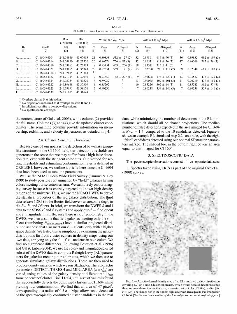
Because one of our goals is the detection of low-mass group-like structures in the Cl 1604 field, our detection thresholds aregenerous in the sense that we may suffer from a high false detec-tion rate, even with the stringent color cuts. Our method for set-ting thresholds and estimating contamination rates is detailed inORELSE I; however, we outline it briefly here since the Cl 1604data have been used to tune the parameters.

We use the NOAO Deep Wide Field Survey (Jannuzi & Dey1999) to study possible contamination by ‘‘field’’ galaxies havingcolors meeting our selection criteria. We cannot rely on our imag-ing survey because it is entirely targeted at known high-densityregions of the universe. Thus, we use the NOAODWFS to derivethe statistical properties of the red galaxy distribution. The thirddata release (DR3) in the Bootes field covers an area of 9 deg2, inthe BW, R, and I filters. In brief, we transform the DWFS R and Idata to the SDSS r 0 and i0 systems and apply our r 0 � i0 color cutand i0 magnitude limit. Because there is no z0 photometry in theDWFS, we then assume that field galaxies meeting only the r 0 �i0 cut (numbering N1color;DWFS) have a similar projected distri-bution as those that also meet our i0 � z0 cuts, only with a higherspace density. We tested this assumption by examining the galaxydistributions far from cluster centers in density maps using ourown data, applying only the r 0 � i0 cut and cuts in both colors.Wefind no significant differences. Following Postman et al. (1996)and Gal & Lubin (2004), we use the color- and magnitude-selectedsubset of the DWFS data to compute Raleigh-Levy (RL) param-eters for galaxies meeting our color cuts, which we then use togenerate simulated galaxy distributions. These are then used toproduce density maps on which we run SExtractor. The SExtractorparameters DETECT_THRESH and MIN_AREA (� ; r2test) arevaried, using values of the galaxy density at different radii rtestfrom the center of cluster C inCl 1604, until a set of values is foundthat successfully detects the confirmed clusters in Cl 1604 whileyielding low contamination. We find that an area of 47 pixel2,corresponding to a radius of 0.3 h�1 Mpc, allows us to detect allof the spectroscopically confirmed cluster candidates in the real

data, while minimizing the number of detections in the RL sim-ulations, which should all be chance projections. The mediannumber of false detections expected in the area imaged for Cl 1604is Nfalse ¼ 1:4, compared to the 10 candidates detected. Figure 3shows an example RL simulated map 2.2� on a side, with the eight‘‘false’’ candidates detected using our optimal SExtractor parame-ters marked. The shaded box in the bottom right covers an areaequal to that imaged for Cl 1604.

3. SPECTROSCOPIC DATA

The spectroscopic observations consist of five separate data sets:

1. Spectra taken using LRIS as part of the original Oke et al.(1998) survey.

TABLE 1

Cl 1604 Cluster Coordinates, Redshifts, and Velocity Dispersions

Within 0.5 h�170 Mpc Within 1.0 h�1

70 Mpc Within 1.5 h�170 Mpc

ID

(1)

Name

(2)

R.A.

(J2000.0)

(deg)

(3)

Decl.

(J2000.0)

(deg)

(4)

N

(5)

zmean

(6)

�(Nagree)

(7)

N

(8)

zmean

(9)

�(Nagree)

(10)

N

(11)

zmean

(12)

�(Nagree)

(13)

A................. Cl 1604+4304 241.08946 43.07613 21 0.89838 532 � 127 (2) 32 0.89861 619 � 96 (3) 36 0.89832 682 � 109 (3)

B................. Cl 1604+4314 241.09890 43.23550 20 0.86574 756 � 83 (3) 32 0.86531 811 � 76 (3) 47 0.86569 767 � 76 (3)

C................. Cl 1604+4316 241.03162 43.26313 8 0.93451 439 � 256 (1) 18 0.93511 313 � 41 (3) a . . . . . .

D................. Cl 1604+4321 241.13865 43.35343 28 0.92351 559 � 171 (2) 53 0.92280 590 � 112 (2) 69 0.92340 668 � 103 (3)

E ................. Cl 1604+4314B 241.02815 43.23343 b . . . . . . . . . . . . . . . . . . . . . . . .F ................. Cl 1605+4322 241.21314 43.37091 7 0.93659 142 � 297 (1) 9 0.93608 173 � 220 (1) 13 0.93532 435 � 129 (2)

G................. Cl 1604+4324 240.93754 43.40520 6 0.89932 c 13 0.90075 409 � 101 (3) 21 0.90210 477 � 152 (3)

H................. Cl 1604+4322 240.89648 43.37309 6 0.85292 c 10 0.85226 302 � 64 (3) 11 0.85243 312 � 57 (3)

I .................. Cl 1603+4323 240.79691 43.39176 5 0.90230 c 7 0.90238 359 � 140 (3) 7 0.90238 359 � 140 (3)

J .................. Cl 1604+4331 240.91905 43.51648 d . . . . . . . . . . . . . . . . . . . . . . . .

a Overlaps cluster B at this radius.b No dispersions measured as it overlaps clusters B and C.c Insufficient redshifts to compute dispersions.d No spectroscopic coverage.

Fig. 3.—Adaptive kernel density map of an RL simulated galaxy distributioncovering 2.2� on a side. Cluster candidates, whichwould be false detections sincethere are no real structures in thismap, aremarkedwith circles of 1.0h�1

70 radius (forz ¼ 0:9). The shaded box in the bottom right covers an area equal to that imaged forCl 1604. [See the electronic edition of the Journal for a color version of this figure.]


2. Additional LRIS spectra taken in 2000 May, covering thearea imaged with COSMIC.

3. DEIMOS spectra covering the same area taken in 2003.4. DEIMOS spectra taken in 2005 and 2006, using color selec-

tion and spanning a larger area imaged with LFC.5. DEIMOS spectra covering the same area as before, but in-

cluding X-ray, radio, Hubble Space Telescope (HST ) AdvancedCamera for Surveys (ACS), and new color-selected sources.

Each sample is described in more detail below, with the layoutof all masks shown in Figure 4.

3.1. LRIS and DEIMOS Observations

The original observations of Cl 1604+4304 and Cl 1604+4321 (clusters A and D) were taken in the late 1990s with LRISon the Keck I and II telescopes and are detailed in Oke et al.(1998), Postman et al. (1998), and Lubin et al. (1998). These ini-tial slit masks targeted all galaxies with R < 23:5 based on ear-lier imaging with LRIS. It is important to note that no colorselection was utilized in selecting galaxies to observe; therefore,blue galaxies at the supercluster redshift are more likely to be ob-served compared to the DEIMOS data discussed below. Redshifts

were measured for 103 and 135 galaxies in the fields of Cl 1604+4304 and Cl 1604+4321, respectively. Imaging of a larger re-gion with COSMIC on the Palomar 200 inch (5 m) telescope wasused to design additional LRIS slit masks, targeting an area includ-ing clusters B and C. Objects with magnitudes down to i ¼ 23:0were included, with priority given to red galaxies. Six additionalLRIS masks with 156 targets were observed in 2000 May. Me-dian velocity errors for the LRIS data are 150 km s�1.

Starting in 2003 May, Cl 1604 was observed with DEIMOSon the Keck II telescope. We briefly describe these observationshere; the details will be provided in a future paper releasing multi-wavelength data, including redshifts, in the Cl 1604 field. Thefirst DEIMOS observations also spanned the region imaged withCOSMIC and are detailed in Gal & Lubin (2004). Galaxies asfaint as i � 24were observed, with higher priority for red galaxiesbased on COSMIC R� i; only 60% of the targeted objects metthe red galaxy color cut.Weused the 1200 linemm�1 grating, blazedat 75008, and 100 slits, resulting in a pixel scale of 0.338 pixel�1,a resolution of �1.78 (68 km s�1), and typical spectral coveragefrom 6385 to 9015 8. Data were reduced using the DEEP2 ver-sion of the spec2d and spec1d data reduction pipelines (Daviset al. 2003). Since the publication of Gal & Lubin (2004), the

Fig. 4.—Layout of spectroscopic observations in the Cl 1604 field. The regions imaged from the ground with COSMIC (red dashed lines) and LFC (green dashedlines) are shown, along with the LRISmasks observed in 2000May as dotted lines. The 11 DEIMOSmasks from the three campaigns discussed in the text are also plotted,along with the locations of the clusters detected from the density map.


DEEP2 team has made available their redshift measurementpipeline zspec (Cooper 2007) and all DEIMOS redshifts have nowbeen obtained using this package. Typical redshift errors using thismethod are 25 km s�1, nearly a factor of 4 improvement over ouroriginal measures.

Using the multiband LFC photometry from Gal et al. (2005),galaxies with 20:5 � i0 � 24:0 were targeted over a larger areabased on both color andmagnitude. FiveDEIMOSmasks, labeledCE1, FG1, FG2, GHF1, and GHF2 in Figure 4, were observed in2005 and 2006 using these ground-based color selection crite-ria. The Cl 1604 supercluster was also the subject of a two-band17-pointing mosaic with the ACS, a two-pointing ACIS-I obser-vation with Chandra (Kocevski et al. 2008), and a Very LargeArray B configuration 1.4 GHz radio map (N. Miller et al. 2008,in preparation). These multiband data were used to design addi-tional DEIMOS masks. The primary sample included X-ray andradio sources within the ACS mosaic and red-sequence galaxiesselected on the basis of the high-precision ACS colors. Secondarysamples includedX-ray and radio sources outside theACSmosaicand bluer galaxieswithin theACSmosaic. Lower priority samplesinclude red galaxies outside the ACS mosaic, then bluer (by asmuch as 0.3 mag) galaxies outside the ACS area, and finally anygalaxy not already selected by the above criteria. We observedthree of these masks in 2007 June.

Figure 4 shows the positions of the LRIS masks observed in2000May, as well as all 11 DEIMOSmasks. The locations of thecluster and group candidates are also marked. This figure makesevident the uneven spectroscopic coverage of the supercluster.Especially noteworthy is the extensive LRIS coverage of clus-ters A andD; because no color selection was used for the originalLRIS masks, the blue (presumably star-forming) populations inthese clusters will be better sampled. Nevertheless, even in re-gions where there is only DEIMOS coverage, �50% of the tar-geted galaxies were outside the red sequence. We explore thedependence of cluster velocity dispersions on the populationsampling in x 4.1.3.

In addition to the targeted objects, numerous serendipitousspectra were found by visual inspection. These objects had theirextraction windows set manually but were otherwise run throughthe same pipelines as the target objects. Two of us (R. G. and B. L.)systematically inspected all of the spec2d -created serendip one-dimensional spectra to determine whether these extractions con-tained genuine serendips and to confirm their redshifts. A significantnumber of serendips (180 extragalactic objects, 138 withQ > 2)were found in our DEIMOS data. Many of these at the super-cluster redshift show strong [O ii] emission and little continuum.These objects represent a different population than the primary tar-gets (red-sequence galaxies) and may impact the velocity disper-sion determination, explored in x 4.1.3.

3.2. Combined Spectroscopy Results

All of the spectroscopic data were combined into a singlemas-ter catalog. For objects observed with both LRIS and DEIMOS,we used the DEIMOS results due to the improved redshift accu-racy with the higher dispersion grism and typically higher signal-to-noise ratio. Serendipitous spectra were matched to photometricobjects from ACS and/or Palomar imaging. In a few cases nocounterpart was found, usually for single emission line spectra,some of which are likely to beLy� emitters at z > 4 (B.C.Lemauxet al. 2008b, in preparation). Each photometric identification wasexamined visually (by R. G.) to check for blends, interacting gal-axies, and misidentifications. A set of flags was added to the cat-alog, identifying whether or not the object was detected and/orblended in either or both of the ACS and Palomar images. The

final catalog contains a total of 1671 unique objects. Of these, thefollowing applies:

1. 1215 are extragalactic objects, of which 1138 have Q ¼ 3or 4.2. 1148 (1089 with Q ¼ 3 or 4) of the above are matched to a

cleanly detected (not blended) photometric object in either theACS or ground-based imaging.3. 140 are stars.4. 427 are in the redshift range of the supercluster (0:84 �

z � 0:96), of which 413 have Q ¼ 3 or 4.5. 417 (404 with Q ¼ 3 or 4) of the supercluster members

have clean photometry.

The top panel of Figure 5 shows the redshift distribution of theQ ¼ 3 or 4 extragalactic objects (solid line), as well as for objectswith Q � 2 (dotted line). The bottom panel shows only the red-shift range of the supercluster (0:84 � z � 0:96) with redshiftbins of �z ¼ 0:001. In addition to a number of clear redshiftpeaks in the supercluster, many intervening structures are no-ticeable, discussed in detail in x 5. We use only the most reliable(Q ¼ 3 or 4) redshifts for all of the analyses presented here.

4. CLUSTER PROPERTIES ANDSUPERCLUSTER STRUCTURE

4.1. Individual Cluster Properties

Nine of the 10 cluster candidates listed in Table 1 have beenextensively mapped in our spectroscopic campaign, with onlycluster J lacking spectroscopic coverage. We use our data set toexamine the redshift distribution around each cluster candidate,both to verify the structures and to measure velocity dispersions.Because of our generous detection threshold, we expect to findstructures consistent with modest sized groups, as well as richerclusters. In some cases, clusters overlap each other even with thesmallest radius used, and almost all clusters have companionswithin 1 h�1

70 Mpc, as seen in Figure 2. The complex superclusterstructure makes separation of individual cluster componentsdifficult and in some cases impossible. Information on both po-sition and velocity must be incorporated; even so, individualclusters or groups may exhibit significant substructure (Dressler& Shectman 1988).

4.1.1. Velocity Dispersions

We use the cluster centers determined by SExtractor from thedensity map when measuring cluster redshifts and velocity dis-persions. We note that the spectroscopic coverage varies greatlyfrom cluster to cluster, as seen in Figure 4.We first construct red-shift histograms within 0.5, 1.0, and 1.5 h�1

70 Mpc projected radiicentered on each cluster. These are plotted in Figure 6 for clus-ters AYI. The shaded region, solid line, and dashed line show theredshift distributionswithin 0.5, 1.0, and 1.5 h�1

70 Mpc, respectively.An initial redshift range (typically spanning �3000 km s�1) foreach cluster is then selected by visual inspection of these plots,attempting to avoid clear redshift peaks from adjacent structures.The extensive overlap between structures results in contami-

nation of the redshift distributions. A good example is cluster C(z � 0:935), where we see numerous galaxies at z � 0:865 withina projected 0.5 h�1

70 Mpc radius. In this case, the redshift separationis large enough to easily distinguish the two populations. Morecomplicated overlaps, such as betweenD and F,where the redshiftseparation is only�z � 0:01, are difficult to resolve. In such cases,neglecting the overlap may lead to overestimation of the velocitydispersion. Conversely, applying strict redshift limits to avoid suchoverlaps can artificially lower the measured dispersion.


For each cluster we follow the procedure described in Gal et al.(2005) and Lubin et al. (2002). After the initial redshift range ischosen, the cosmologically corrected velocities relative to the me-dian cluster redshift are calculated for each galaxywithin the threeradii. The initial velocity windows are typically �3000 km s�1,sufficiently broad to avoid biasing the dispersion estimates tolower values. These distributions are iteratively clipped at 3 �,where � is the biweight dispersion computed by ROSTAT (Beerset al. 1990). Typically from zero to two galaxies are excludedfrom each cluster by this clipping. The final dispersions are com-puted using the biweight estimate of the scale, with errors takenfrom the jackknife confidence interval on the biweight scale. Thesehave been shown to be well behaved under most circumstances formodest sample sizes (Beers et al. 1990).

Contamination from fore/background clusters, groups, andfilaments could bias the measured velocity dispersions and theirassociated errors when using ROSTAT (Andreon 2008). Wehave used quite stringent spatial and redshift cuts to establish thestarting ranges for velocity dispersion measurement, which re-duces the contamination. We also examined the agreement be-tween the 3 � clipped standard dispersion, the biweight estimateof the scale, and the gapped estimator, noting how many (out ofthree maximum) of these estimators agree within the quoted er-rors. The results are presented in Table 1. Columns (5), (8), and(11) give the number of spectroscopically confirmed memberswithin 0.5, 1.0, and 1.5 h�1

70 Mpcprojected radii, respectively. Thesenumbers include only those galaxies used to compute the velocitydispersions within each radius. Columns (6), (9), and (12) provide

the median redshift for each cluster within each of the three radii,while columns (7), (10), and (13) list the computed velocity dis-persions and their errors. Columns (7), (10), and (13) also include,in parentheses, the number of different dispersion estimators thatagree within the errors. Despite having fewer galaxies, we wouldprefer the final velocity dispersions to be those measured within0.5 h�1

70 Mpc, since the smaller radius reduces contamination fromoverlapping clusters. However, only clusters AYD have sufficientmembers within this small radius to compute dispersions, so wequote the dispersions using the 1.0 h�1

70 Mpc radius throughout.The final redshift intervals used for this radius are shown in Figure 6as the vertical lines near the top of each panel. The sole exception iscluster E, which appears to be a superposition of components re-lated to clusters B and C. Therefore, we measure no velocity dis-persion and do not show its color-magnitude diagrams (CMDs).

4.1.2. Velocity Dispersions, Errors, and the Effect of Interlopers

If we assume that the velocity dispersion errors quoted inTable 1 are due purely to sample size, then we would expect theerrors to decrease with the square root of the number of galaxiessampled. This is almost exactly true for clusters A and D, and thequoted dispersions using different radii all agree within 1 �. Forcluster B, the three quoted dispersions agree very well, even thoughthe estimated error remains nearly constant with sample size. Forthe remaining structures, which all havemuch sparser sampling andappear to be intrinsically poorer, the effects of small numbers andcontamination from interlopers make reliable dispersion estimatesimpossible. A good example is cluster G, where the estimated error

Fig. 5.—Redshift distribution in the Cl 1604 field. The top panel shows all extragalactic objects (dotted line) and only those with high-redshift quality (solid line). Thebottom panel focuses on the supercluster redshift range with redshift bins of �z ¼ 0:001.


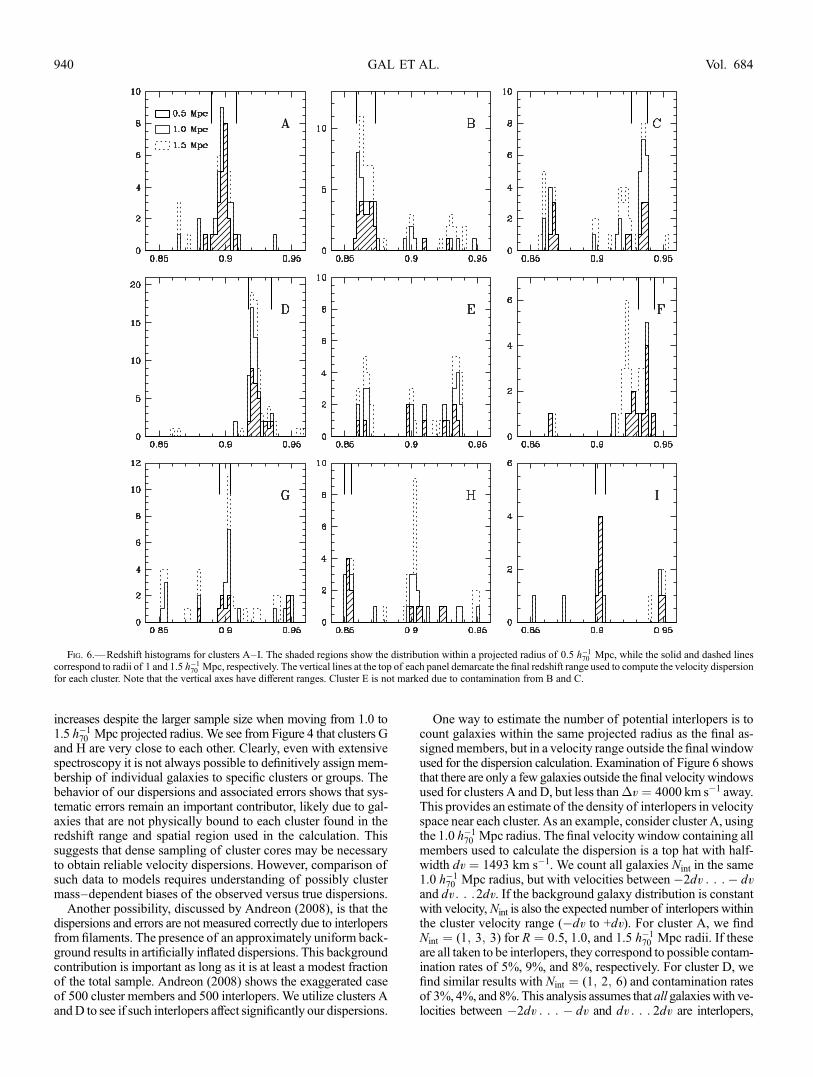
increases despite the larger sample size when moving from 1.0 to1.5 h�1

70 Mpc projected radius. We see from Figure 4 that clusters Gand H are very close to each other. Clearly, even with extensivespectroscopy it is not always possible to definitively assign mem-bership of individual galaxies to specific clusters or groups. Thebehavior of our dispersions and associated errors shows that sys-tematic errors remain an important contributor, likely due to gal-axies that are not physically bound to each cluster found in theredshift range and spatial region used in the calculation. Thissuggests that dense sampling of cluster cores may be necessaryto obtain reliable velocity dispersions. However, comparison ofsuch data to models requires understanding of possibly clustermassYdependent biases of the observed versus true dispersions.

Another possibility, discussed by Andreon (2008), is that thedispersions and errors are not measured correctly due to interlopersfrom filaments. The presence of an approximately uniform back-ground results in artificially inflated dispersions. This backgroundcontribution is important as long as it is at least a modest fractionof the total sample. Andreon (2008) shows the exaggerated caseof 500 cluster members and 500 interlopers. We utilize clusters AandD to see if such interlopers affect significantly our dispersions.

One way to estimate the number of potential interlopers is tocount galaxies within the same projected radius as the final as-signedmembers, but in a velocity range outside the final windowused for the dispersion calculation. Examination of Figure 6 showsthat there are only a few galaxies outside the final velocity windowsused for clusters A and D, but less than�v ¼ 4000 km s�1 away.This provides an estimate of the density of interlopers in velocityspace near each cluster. As an example, consider cluster A, usingthe 1.0 h�1

70 Mpc radius. The final velocity window containing allmembers used to calculate the dispersion is a top hat with half-width dv ¼ 1493 km s�1. We count all galaxies Nint in the same1.0 h�1

70 Mpc radius, but with velocities between �2dv : : :� dvand dv : : :2dv. If the background galaxy distribution is constantwith velocity,Nint is also the expected number of interlopers withinthe cluster velocity range (�dv to +dv). For cluster A, we findNint ¼ (1; 3; 3) for R ¼ 0:5, 1.0, and 1.5 h�1

70 Mpc radii. If theseare all taken to be interlopers, they correspond to possible contam-ination rates of 5%, 9%, and 8%, respectively. For cluster D, wefind similar results with Nint ¼ (1; 2; 6) and contamination ratesof 3%, 4%, and 8%.This analysis assumes that all galaxieswith ve-locities between �2dv : : : � dv and dv : : : 2dv are interlopers,

Fig. 6.—Redshift histograms for clusters AYI. The shaded regions show the distribution within a projected radius of 0.5 h�170 Mpc, while the solid and dashed lines

correspond to radii of 1 and 1.5 h�170 Mpc, respectively. The vertical lines at the top of each panel demarcate the final redshift range used to compute the velocity dispersion

for each cluster. Note that the vertical axes have different ranges. Cluster E is not marked due to contamination from B and C.


thus providing an estimate of the maximum effect that they couldhave.

To see if the presence of such objects could effect the velocitydispersions, we perform a Monte Carlo simulation with clus-ters A and D, using all three projected radii. We remove Nint gal-axies from the velocity range�dv: : :dv. One galaxy is removedin each velocity bin of width 2dv/Nint, ensuring that the likelihoodof removal is flat across the entire velocity range, correspondingto contamination by a constant background. The velocity disper-sion and associated errors are recomputed using the new sample,and this procedure is repeated 1000 times for each cluster and ra-dius combination.We compute themean velocity dispersion (usingthe biweight dispersion estimator from ROSTAT) and mean error( jackknife of the biweight from ROSTAT) for each cluster andradius combination from the 1000Monte Carlo runs. We then ex-amine (1) the difference between these velocity dispersions andthe original estimates and (2) the rms scatter within the 1000MonteCarlo runs. We find that the velocity dispersions calculated afterremoving potential interlopers are only 1%Y5% lower than theinitial estimates. As an example, the original dispersions for clus-ter A using the three radii are 532, 619, and 682 km s�1. Theinterloper-corrected estimates are 532, 595, and 647 km s�1,corresponding to reductions of 0%, 4.0%, and 5.4%, respectively.The scatter among the Monte Carlo runs is 10Y50 km s�1, de-pending on the cluster and radius used. Adding this in quadratureto the already quoted error estimates would only increase the er-rors by �10%. These results demonstrate that there is little biasin our velocity dispersions due to interlopers.

4.1.3. Dependence of Velocity Dispersionson Sampling and Galaxy Colors

In addition to the possibility of interlopers, the spectroscopicsampling is significantly variable from cluster to cluster, as de-scribed in x 3. This is especially true for clusters A and D, whichhave extensive LRIS data where no color cuts were applied. Be-cause the measured velocity dispersions for these (and other)clusters in Cl 1604 have decreased significantly compared to ourand others’ earlier observations (Gal&Lubin 2004; Postman et al.1998, 2001), we examine how the sampling (by instrument and bycolor) affects the current results.

First, for clusters A and D, we simply excluded the LRIS red-shifts and measured their velocity dispersions using only theDEIMOS data. The DEIMOS data have significantly smaller red-shift errors, and using only the DEIMOS data makes the instru-mental sampling similar for all of the clusters.We use the 1 h�1

70 Mpcradius for this test to maintain a significant number of galaxies.Cluster A has 26 galaxies with Q > 2 DEIMOS redshifts, yield-ing a velocity dispersion � ¼ 691 � 103 km s�1, consistent withthe results including LRIS (32 galaxies, 619 � 96 km s�1). Forcluster D, theDEIMOS-only dispersion is� ¼ 445 � 134 km s�1

from29galaxies, compared to� ¼ 590 � 112 kms�1 from53 gal-axies when LRIS data are included. These values are also con-sistent within the errors, although the lowered dispersion whenonly DEIMOS data are used may be due to the large number ofLRIS redshifts excluded. The LRIS-observed galaxies are, onaverage, bluer than the DEIMOS-observed ones and may there-fore have a different dispersion. We note, however, that nearlyhalf the DEIMOS targets are also outside the red sequence. Weconclude that the inclusion of LRIS data for some clusters doesnot significantly alter our results.

We further examined if the computed dispersion is differentfor red-sequence galaxies than for the cluster population as awhole.Such segregation was already shown by Zabludoff & Franx (1993),who found higher dispersions for late-type galaxies than for early-

type galaxies in rich, low-redshift clusters. This effect should beeven more pronounced at high redshift, where the clusters areless evolved. Furthermore, since there is a color-density relation-ship, using only the red galaxies should reduce the contributionof infalling groups/filaments at the cost of smaller sample size.We applied the same color limits used for the density mapping[1:0 � (r 0 � i0) � 1:4, 0:6 � (i0 � z0) � 1:0] and a magnitudelimit of i0 � 24:0 to the spectroscopic samples in each cluster. Onlyclusters A, B, and D have sufficient (although still small) numbersof red galaxies for this exercise. Using the 1 h�1

70 Mpc radius tomaintain a significant number of galaxies, we find the following:

1. Cluster A: full sample 32 galaxies, � ¼ 619 � 96 km s�1;color cut 18 galaxies, � ¼ 327 � 62 km s�1.

2. Cluster B: full sample 32 galaxies, � ¼ 811 � 76 km s�1;color cut 12 galaxies, � ¼ 778 � 127 km s�1.

3. Cluster D: full sample 53 galaxies, � ¼ 590 � 112 km s�1;color cut 16 galaxies, � ¼ 338 � 71 km s�1.

In all three cases, the red galaxies have a lower velocity dis-persion. For cluster A the difference is 3.0 �, while for cluster Dit is only 2.2 �, and less than 1 � for cluster B. As shown above,these changes are not the result of instrumental coverage (DEIMOSor LRIS), so the differences must reflect the properties of the dis-tinct galaxy populations. It is interesting to note that our Chandraobservations find cluster A to be the most X-rayYluminous sys-tem in the supercluster, exhibiting a relaxed and well-establishedintracluster medium (Kocevski et al. 2008). If the system formedat an earlier epoch than clusters B and D, it is expected that theprimordial red galaxy population would have had more time tofully virialize and establish a much different dispersion than anyinfalling blue galaxy population. The lack of a significant dif-ference in the velocity dispersions of blue and red galaxies incluster B, and to a lesser extent cluster D, may be further evidencethat these systems are undergoing collapse or possiblemerger pro-cesses. These results again suggest that one must exercise cautionboth when selecting galaxies for spectroscopic follow-up usingcolors and when interpreting the resulting cluster velocity dis-persions. Our sample is extremely limited but is one of the first tohave so many cluster members at redshifts near unity. The factthat the pattern of velocity dispersion as a function of galaxy coloris not the same from cluster to cluster may imply that follow-up ofonly red-sequence galaxies might yield biased or inconsistentresults, especially if the red versus blue galaxy dispersion dependson the cluster mass or formation epoch. This could also be true ifonly the most luminous cluster galaxies are used since they aremuch more likely to have red colors. Larger samples with deepspectroscopy of clusters in various evolutionary stages will benecessary to clarify these findings.

The velocity dispersions computed for clusters A and D, usingall galaxies within 0.5 or 1 h�1

70 Mpc radii, are a factor of 2 belowthe initial estimates from Postman et al. (1998, 2001). The �-valuesderived here would place these clusters closer to the LX-� rela-tion, alleviating the X-ray underluminosity discussed in Lubinet al. (2004). This consistency makes it tempting to assume thatthese are the correct dispersions to use; however, the morpho-logical and/or color sampling is not the same from cluster tocluster (due to both sampling differences and population varia-tions), and the X-ray luminosities may also be unreliable due topoint-source contamination. These results clearly require detailedcomparison to simulations to see what population mix is best forproducing reliable velocity dispersions that trace the gravitat-ing halo mass. Simplistic approaches to measuring cluster dis-persions, especially at an epoch when they are still accretingsignificant portions of their final galaxy (and mass) content, are


not likely to be reliable except for the most massive evolvedsystems.

4.1.4. Substructure

To better understand the individual cluster structures and pos-sible contamination from neighboring clusters and filaments, weexamined the spectroscopic coverage and position-velocity dis-tributions within each cluster. These are shown in Figure 7 for allclusters except E (which has no clear redshift peak) and J (whichhas no spectroscopic coverage). There are two panels for each

cluster, each covering an area of 3.2 h�170 Mpc on a side. The left

panels show all galaxies with 20:5 < i0 < 24 as small black dots.Essentially, these are all possible spectroscopic targets in the fieldregardless of priority. Red galaxies used tomake the density mapare shown as larger red dots. The concentrations in the centers ofmost clusters are evident, and in later DEIMOSmasks these wereprioritized. Black squares outline the galaxies with spectroscopicredshifts. Spectroscopic targets that met the density map color cri-teria are almost always cluster members, highlighting the efficiencyof our color cuts in selecting supercluster members. Clusters A

Fig. 7.—Spectroscopic coverage and position-velocity diagrams for eight clusters in Cl 1604. There are two panels for each cluster, each covering an area of 3.2 h�170 Mpc

on a side. The left panels show all galaxieswith 20:5 < i0 < 24 as small black dots, while red galaxies used tomake the densitymap are shown as larger red dots. Black squaresoutline the spectroscopic targets. The right panels for each cluster plot all galaxies in the supercluster redshift range (0:84 � z � 0:96) as small black dots. The finalmembers ofeach cluster are then circled, with red circles for galaxies with higher recession velocities than the clustermean, and blue for those galaxies with lower velocities. The circles arescaled by vgal/�clus, with the scaling shown in the lower right corner of each panel. In both panels, the three large circles correspond to radii of 0.5, 1.0, and 1.5 h

�170 Mpc, used to

measure velocity dispersions.


and D have very dense coverage because they were the first to bediscovered by Gunn et al. (1986) and were the targets of initialLRIS spectroscopy. The three large circles correspond to radii of0.5, 1.0, and 1.5 h�1

70 Mpc, used to measure velocity dispersions.The right panels for each cluster plot all galaxies in the super-cluster redshift range (0:84 � z � 0:96) as small black dots. Thefinal members of each cluster (as determined using ROSTATwithin the 1.5 h�1

70 Mpc radius) are then circled. Red circles areused for galaxies with higher recession velocities than the clustermean, while blue circles show those blueshifted relative to theclustermean.The circle sizes are scaled by the ratio of the galaxies’clustercentric radial velocity to the cluster’s velocity dispersion,vgal/�clus. The corresponding velocity dispersion is shown in thelower right corner of each panel, alongwith a circle for vgal ¼ �clus.

Examination of Figure 7 demonstrates that even the very wellsampled clusters (A, B, and D), with over 30 members within a 1h�170 Mpc radius, show visual evidence for substructure. Cluster

D in particular appears very elongated in the northeast-southwestdirection. Cluster B shows velocity segregation, which could beinterpreted as either substructure or a triaxial cluster, elongatedin the radial direction and oriented at a slight angle to the line ofsight. To quantify the amount of substructure, we performedDressler & Shectman (1988) tests on clusters A, B, and D usingthe spectroscopically confirmed members within a 1.0 h�1

70 Mpcradius (32, 32, and 53 galaxies, respectively). Also known as the� or DS test (Pinkney et al.1996), this statistic looks for velocitysubstructure among galaxies near each other in projection as anindicator of merging components. The DS statistic was shownby Pinkney et al. (1996) to be the most sensitive of the five dif-ferent substructure estimators they examined and works well evenfor moderate samples with only �30 velocities per cluster. Thistest indicates no substructure in cluster A, consistent with its ap-pearance in Figure 7. Cluster B, although showing two velocitysubclumps (Fig. 6), has no significant substructure based on theDS test. This may be the result of having two subclumps verywell aligned along the line of sight, a situation to which the DStest is not sensitive. Cluster D has the highest likelihood ofsubstructure, with the null hypothesis (no substructure) rejected

at the 93% confidence level. This is consistent with the evidentelongation at an angle to the line of sight and the velocity seg-regation between the northeastern and southeastern parts of thecluster.

Recent work using both optical and X-ray data (Sereno et al.2006; Paz et al. 2006; Plionis et al. 2006; De Filippis et al. 2005)has shown that many clusters and groups are quite strongly triaxial,consistent with large simulations such as those of Jing & Suto(2002). In addition, the Cl 1604 supercluster is extremely elon-gated along the line of sight, and we expect, based on Hubblevolume simulations, that the clusters will be aligned with thesupercluster (Lee & Evrard 2007). Further understanding of thecluster dynamicswill require detailed comparison to largeN-bodysimulations, as well as modeling of the Cl 1604 supercluster inparticular.

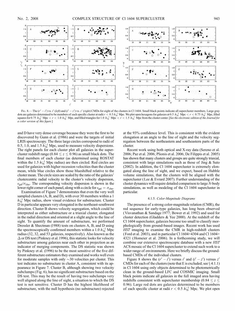
4.1.5. Color-Magnitude Diagrams

The presence of a strong color-magnitude relation (CMR), thered sequence for early-type galaxies, has long been observed(Visvanathan & Sandage 1977; Bower et al. 1992) and used forcluster detection (Gladders & Yee 2000). At the redshift of theCl 1604 supercluster, galaxies become too small to classify mor-phologically from ground-based images. Recent work has usedHST imaging to examine the CMR in high-redshift clusters(Ford et al. 2003), and in particular Cl 1604+4304 and Cl 1604+4321 (Homeier et al. 2006). In a forthcoming study, we willcombine our extensive spectroscopic database with a new HSTACSmosaic of the Cl 1604 supercluster to extend such work to awider range of environments. Here we briefly discuss the ground-based CMDs of the individual clusters.

Figure 8 shows the (r 0 � i0) versus i0 and (i0 � z0) versus z0

CMDs for each of the clusters (note that E is excluded; see x 4.1.1)in Cl 1604 using only objects determined to be photometricallyclean in the ground-based LFC and COSMIC imaging. Smallblack points indicate all galaxies in the full imaged area havingredshifts consistent with supercluster membership (0:84 � z �0:96). Large red dots are galaxies determined to be membersof each specific cluster at radii r < 0:5 h�1

70 Mpc. We plot open

Fig. 8.—The (r 0 � i0) vs. i0 (left) and (i0 � z0) vs. z0 (right) CMDs for eight of the clusters in Cl 1604. Small black points indicate all supercluster members. Large graydots are galaxies determined to bemembers of each specific cluster at radii r < 0:5 h�1

70 Mpc.We plot open hexagons for galaxies at 0:5 h�170 Mpc < r < 0:75 h�1

70 Mpc, filledsquares for 0:75 h�1

70 Mpc < r < 1:0 h�170 Mpc, and filled triangles for 1:0 h�1

70 Mpc < r < 1:5 h�170 Mpc from the cluster center. [See the electronic edition of the Journal for

a color version of this figure.]


hexagons for galaxies at 0:5 h�170 Mpc < r < 0:75 h�1

70 Mpc,filled squares for 0:75 h�1

70 Mpc < r < 1:0 h�170 Mpc, and filled

triangles for 1:0 h�170 Mpc < r < 1:5 h�1

70 Mpc from the clustercenter.

First, we note that the photometric errors are significant forfainter galaxies. At i0 � 24, for instance, the typical error is 0.1mag;added in quadrature with another band, we expect at least 0.15magof scatter at i0 � 24 from photometric uncertainties alone. Theintrinsic width of the red sequence, due to age differences at fixedgalaxy mass, is only �0.05 mag in clusters at z � 1 (Homeieret al. 2006; Mei et al. 2006), similar to that observed locally(McIntosh et al. 2005). The expected slope of the red sequence, aconsequence of metallicity changeswith galaxymass, is also small,of order �0.05 (Kodama & Arimoto 1997). Thus, our ground-based observations are not sufficiently accurate to measure thesequantities.

Nevertheless, a few general observations are possible. The redsequence is most prominent in clusters A and B, which also havethe highest velocity dispersions, consistent with the morphology-density and color-density relations (Dressler 1980; Smith et al.2005; Nuijten et al. 2005; Cooper 2007) and its disappearance inlow-density environments by z � 1 (Tanaka et al. 2004). Cluster D,with a velocity dispersion only 5% lower than cluster A, shows adistinctly less pronounced red sequence. This is illustrated inFigure 9, which shows the distribution of r 0 � i0 colors for spec-troscopically confirmed members of clusters A and D. The leftpanel shows galaxies with r 0 � 23:4, the depth of the completeLRIS spectroscopy in A and D. At these magnitudes, red galaxieshave i0 � 22:6, with photometric errors of �0.04 mag in r 0 and�0.03 mag in i0, or color errors of �0.05 mag. The right panelshows fainter galaxies, with 23:4 < r 0 < 25, where the errors aremuch larger. The solid histograms indicate galaxies in A, whilethe dotted line is for cluster D. The excess of bluer [(r 0 � i0) �0:9] galaxies in cluster D is evident, especially in the fainterpopulation.

Looking at the left panel, cluster A has 11 luminous red (1:0 �r 0 � i0 � 1:4) galaxies, while cluster D (Cl 1604+4321), althoughapparently rich, has only six. If we examine the most luminousobjects, the brightest red galaxy in D has r 0 ¼ 22:985; cluster Ahas five more luminous galaxies, extending to r 0 ¼ 22:18. The

lack of luminous red galaxies coupled with the presence of nu-merous bluer galaxies in D results in a dilution of the red sequence,making it appear much less prominent than in cluster A. ClustersA and D have magnitude-limited spectroscopy for all objectswith R < 23:5 from the Oke et al. (1998) LRIS fields, covering a60 ; 80 area (2:8 ; 3:7 h�1

70 Mpc) around each cluster, so the dif-ferences in the luminous galaxy populations between A and Dare certainly real and not selection effects.The absence of luminous galaxies in D is also not an effect of

simply having fewer galaxies as a result of its lower velocity dis-persion (mass); cluster A has 1.8 times as many objects withr 0 < 23:4 and 1:0 � (r 0 � i0) � 1:4, while wewould expect only�10% more if we assumeM / �2 and Ngals / M . The discrep-ancy only gets worse if we look at the most luminous galaxies(r 0 � 23:0), where there are 5 times more in A than in D. To ex-plain this as purely a result of A’s large mass, we would have toincrease the dispersion of A by 2 � while at the same timedecreasing D’s dispersion by 2 �, resulting in a mass ratio of 4.8,comparable to, but still lower than, the factor of 5 difference inluminous red galaxies.Similarly, the fainter galaxy population differences between A

and D are also physical, as they are sampled by both second-epoch LRIS and later DEIMOS slit masks, with similar cover-age. Our findings are consistent with theHST results of Homeieret al. (2006), who had fewer redshifts but more precise photom-etry. Combinedwith its elongated morphology, these data suggestthat Cl 1604+4321 (D) is a cluster in the process of formation andtherefore has not yet had time to build up its red sequence andassemble massive red galaxies. The remaining structures have in-sufficient spectral coverage or too fewmembers with clean ground-based imaging to make conclusive statements about their galaxypopulations.However, it is clear that many galaxies in the supercluster are

associated not with the individual clusters but with the con-necting filaments instead. This implies that studies of the clusterCMR at high redshift that rely on purely photometric data mayoverestimate the width of the red sequence due to contaminationby dynamically dissociated galaxies. Estimates of the blue gal-axy fraction may be similarly compromised. Studies of low-redshift superclusters have also found that�30% of supercluster

Fig. 9.—Distribution of r 0 � i0 colors for spectroscopically confirmed members of clusters A and D. The left panel shows galaxies with r 0 � 23:4, the depth of thecomplete LRIS spectroscopy in A and D. The right panel shows fainter galaxies, with 23:4 < r 0 < 25. The solid histograms indicate galaxies in A, while the dotted line isfor cluster D. The excess of bluer [(r 0 � i0) � 0:9] galaxies and lack of luminous red galaxies in cluster D are evident.


members are not associated with specific clusters (Small et al.1998); this fraction will only increase at larger look-back times asthe structures are less collapsed.

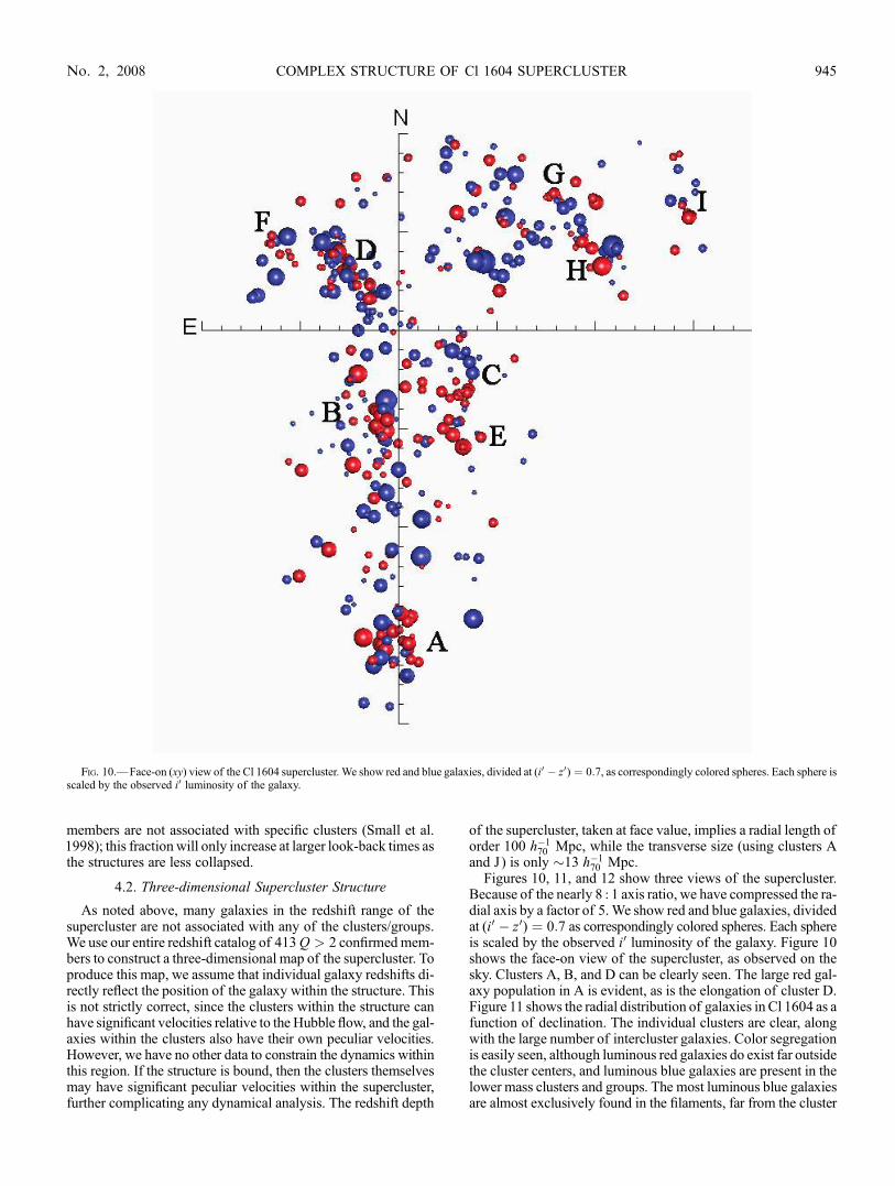
4.2. Three-dimensional Supercluster Structure

As noted above, many galaxies in the redshift range of thesupercluster are not associated with any of the clusters/groups.We use our entire redshift catalog of 413Q > 2 confirmedmem-bers to construct a three-dimensional map of the supercluster. Toproduce this map, we assume that individual galaxy redshifts di-rectly reflect the position of the galaxy within the structure. Thisis not strictly correct, since the clusters within the structure canhave significant velocities relative to the Hubble flow, and the gal-axies within the clusters also have their own peculiar velocities.However, we have no other data to constrain the dynamics withinthis region. If the structure is bound, then the clusters themselvesmay have significant peculiar velocities within the supercluster,further complicating any dynamical analysis. The redshift depth

of the supercluster, taken at face value, implies a radial length oforder 100 h�1

70 Mpc, while the transverse size (using clusters Aand J) is only �13 h�1

70 Mpc.Figures 10, 11, and 12 show three views of the supercluster.

Because of the nearly 8 : 1 axis ratio, we have compressed the ra-dial axis by a factor of 5.We show red and blue galaxies, dividedat (i0 � z0) ¼ 0:7 as correspondingly colored spheres. Each sphereis scaled by the observed i0 luminosity of the galaxy. Figure 10shows the face-on view of the supercluster, as observed on thesky. Clusters A, B, and D can be clearly seen. The large red gal-axy population in A is evident, as is the elongation of cluster D.Figure 11 shows the radial distribution of galaxies in Cl 1604 as afunction of declination. The individual clusters are clear, alongwith the large number of intercluster galaxies. Color segregationis easily seen, although luminous red galaxies do exist far outsidethe cluster centers, and luminous blue galaxies are present in thelower mass clusters and groups. The most luminous blue galaxiesare almost exclusively found in the filaments, far from the cluster

Fig. 10.—Face-on (xy) view of the Cl 1604 supercluster. We show red and blue galaxies, divided at (i0 � z0) ¼ 0:7, as correspondingly colored spheres. Each sphere isscaled by the observed i0 luminosity of the galaxy.


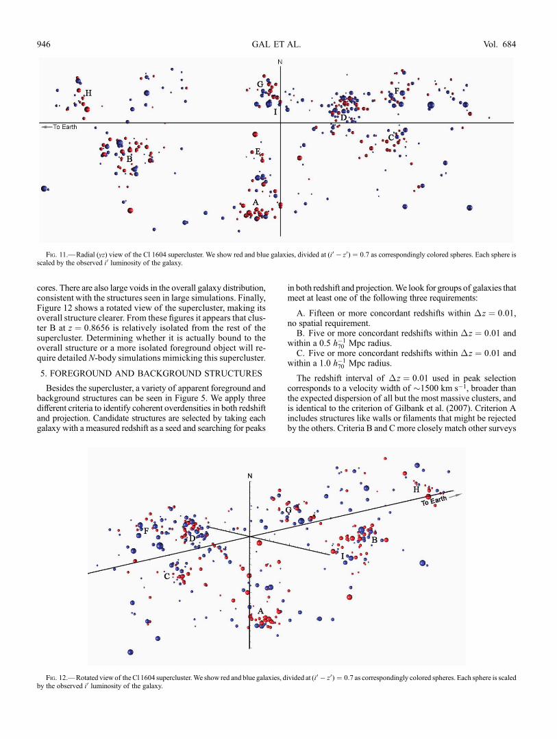
cores. There are also large voids in the overall galaxy distribution,consistent with the structures seen in large simulations. Finally,Figure 12 shows a rotated view of the supercluster, making itsoverall structure clearer. From these figures it appears that clus-ter B at z ¼ 0:8656 is relatively isolated from the rest of thesupercluster. Determining whether it is actually bound to theoverall structure or a more isolated foreground object will re-quire detailed N-body simulations mimicking this supercluster.

5. FOREGROUND AND BACKGROUND STRUCTURES

Besides the supercluster, a variety of apparent foreground andbackground structures can be seen in Figure 5. We apply threedifferent criteria to identify coherent overdensities in both redshiftand projection. Candidate structures are selected by taking eachgalaxy with a measured redshift as a seed and searching for peaks

in both redshift and projection.We look for groups of galaxies thatmeet at least one of the following three requirements:

A. Fifteen or more concordant redshifts within �z ¼ 0:01,no spatial requirement.B. Five or more concordant redshifts within �z ¼ 0:01 and

within a 0.5 h�170 Mpc radius.

C. Five or more concordant redshifts within �z ¼ 0:01 andwithin a 1.0 h�1

70 Mpc radius.

The redshift interval of �z ¼ 0:01 used in peak selectioncorresponds to a velocity width of �1500 km s�1, broader thanthe expected dispersion of all but the most massive clusters, andis identical to the criterion of Gilbank et al. (2007). Criterion Aincludes structures like walls or filaments that might be rejectedby the others. Criteria B and C more closely match other surveys

Fig. 11.—Radial (yz) view of the Cl 1604 supercluster. We show red and blue galaxies, divided at (i0 � z0) ¼ 0:7 as correspondingly colored spheres. Each sphere isscaled by the observed i0 luminosity of the galaxy.

Fig. 12.—Rotated view of the Cl 1604 supercluster.We show red and blue galaxies, divided at (i0 � z0) ¼ 0:7 as correspondingly colored spheres. Each sphere is scaledby the observed i0 luminosity of the galaxy.


that do spectroscopic follow-up in a limited spatial region aroundcandidate clusters. Criterion A selects a total of 18 redshift peaksoutside the supercluster redshift range. Criterion B selects sixpeaks, all of which are also found by A, while criterion C selects13 peaks, 11 of which are also selected byA.Although these can-didate structures are chosen based on well-defined criteria, theuneven spatial coverage, survey depth, color selection, and biasessuch as easier identification of emission-line objects imply that

this sample is neither complete nor unbiased (in redshift or galaxytype).

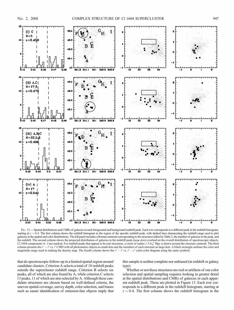
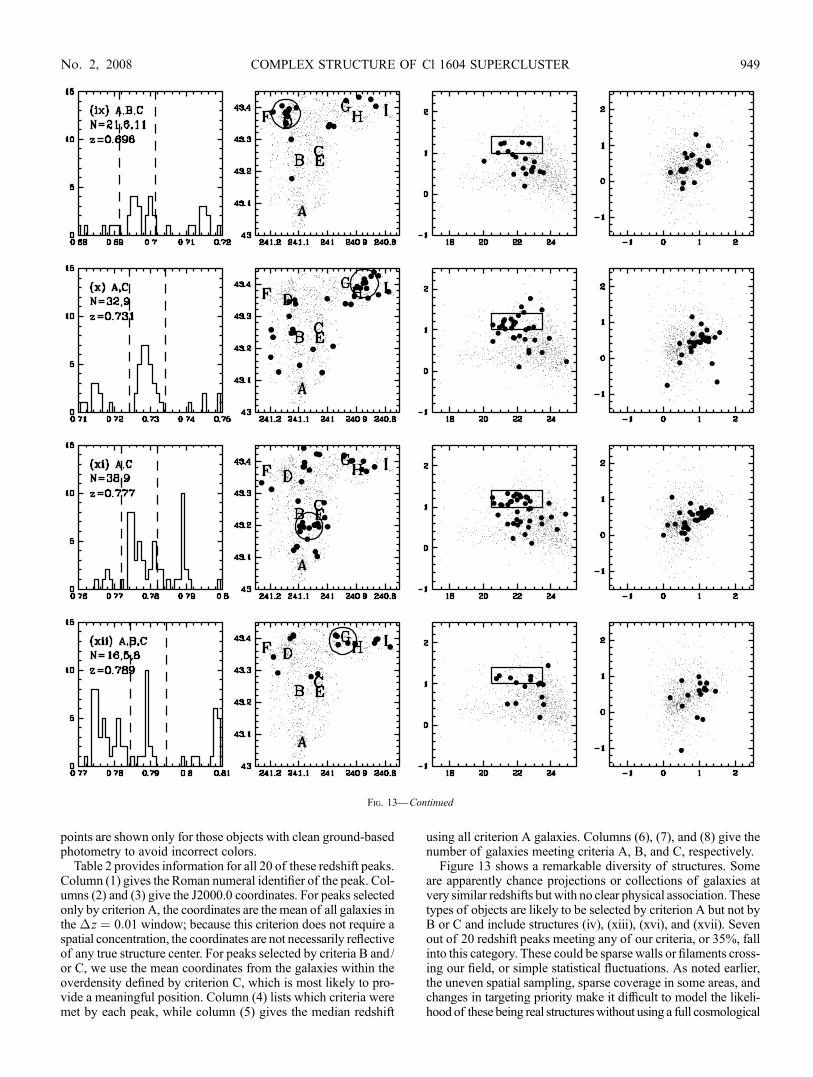
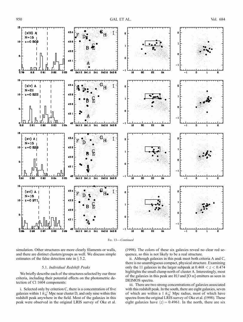
Whether or not these structures are real or artifacts of our colorselection and spatial sampling requires looking in greater detailat the spatial distributions and CMRs of galaxies in each appar-ent redshift peak. These are plotted in Figure 13. Each row cor-responds to a different peak in the redshift histogram, starting atz � 0:4. The first column shows the redshift histogram in the

Fig. 13.—Spatial distributions and CMRs of galaxies in each foreground and background redshift peak. Each row corresponds to a different peak in the redshift histogram,starting at z � 0:4. The first column shows the redshift histogram in the region of the specific redshift peak, with dashed lines demarcating the redshift range used to plotgalaxies in the spatial and color distributions. The left panel includes a Romannumeral corresponding to the structures tallied in Table 2, the number of galaxies in the peak, andthe redshift. The second column shows the projected distribution of galaxies in the redshift peak (large dots) overlaid on the overall distribution of spectroscopic objects.Cl 1604 components AYJ are marked. For redshift peaks that appear to be real structures, a circle of radius 1.5 h�1

70 Mpc is drawn around the structure centroid. The thirdcolumn presents the r 0 � i0 vs. i0 CMDwith all photometric objects as small dots and the members of each structure as large dots. A black rectangle outlines the color andmagnitude range used in making the density map. The fourth column shows the r 0 � i0 vs. i0 � z0 color-color diagram using the same symbols.


region of the specific redshift peak, with dashed lines demar-cating the initial redshift range�z ¼ 0:01 used to select the peakwith criterion A. The left panel includes a Roman numeral cor-responding to the structures tallied in Table 2, followed by lettersdenoting which criteria are met by the peak. We also show thenumber of galaxies in the peak based on each of the criteria bywhich it is selected. The median redshift is included, again usingall criterion A galaxies. Column (1) shows the projected distribu-tion of galaxies in the redshift peak (within�z ¼ 0:01) as largedots overlaid on the overall distribution of spectroscopic objects.The locations of clusters AYI are labeled. If there is an apparentprojected overdensity of objects as defined by criteria B and/orC, we plot a circle of radius 1.0 h�1

70 Mpc around the structure

centroid, using the mean positions of the galaxies within theapparent projected overdensity (except for structure [vii], as de-tailed below). When there are multiple spatial overdensities in asingle redshift peak meeting criteria B and/or C, we show onlythe one with the most members. Column (3) presents the (r 0 � i0)versus i0 CMD with all photometric objects as small black dotsand the structure members (based on criterion A) as large dots.The color and magnitude limits for galaxies used in making thedensity map are shown as the black rectangle in these panels; thehighest priority DEIMOS targets have these colors but extendedto i0 ¼ 24. Column (4) shows the (r 0 � i0) versus (i0 � z0) color-color diagram using the same symbols. Redshifts and positionsare shown for all spectroscopic objects, while photometric data

Fig. 13—Continued


points are shown only for those objects with clean ground-basedphotometry to avoid incorrect colors.

Table 2 provides information for all 20 of these redshift peaks.Column (1) gives the Roman numeral identifier of the peak. Col-umns (2) and (3) give the J2000.0 coordinates. For peaks selectedonly by criterion A, the coordinates are the mean of all galaxies inthe �z ¼ 0:01 window; because this criterion does not require aspatial concentration, the coordinates are not necessarily reflectiveof any true structure center. For peaks selected by criteria B and/or C, we use the mean coordinates from the galaxies within theoverdensity defined by criterion C, which is most likely to pro-vide a meaningful position. Column (4) lists which criteria weremet by each peak, while column (5) gives the median redshift

using all criterion A galaxies. Columns (6), (7), and (8) give thenumber of galaxies meeting criteria A, B, and C, respectively.

Figure 13 shows a remarkable diversity of structures. Someare apparently chance projections or collections of galaxies atvery similar redshifts butwith no clear physical association. Thesetypes of objects are likely to be selected by criterion A but not byB or C and include structures (iv), (xiii), (xvi), and (xvii). Sevenout of 20 redshift peaks meeting any of our criteria, or 35%, fallinto this category. These could be sparse walls or filaments cross-ing our field, or simple statistical fluctuations. As noted earlier,the uneven spatial sampling, sparse coverage in some areas, andchanges in targeting priority make it difficult to model the likeli-hood of these being real structureswithout using a full cosmological

Fig. 13—Continued


simulation. Other structures are more clearly filaments or walls,and there are distinct clusters/groups as well. We discuss simpleestimates of the false detection rate in x 5.2.

5.1. Individual Redshift Peaks

Webriefly describe each of the structures selected by our threecriteria, including their potential effects on the photometric de-tection of Cl 1604 components:

i. Selected only by criterion C, there is a concentration of fivegalaxies within 1 h�1

70 Mpc near cluster D, and only nine within thisredshift peak anywhere in the field. Most of the galaxies in thispeak were observed in the original LRIS survey of Oke et al.

(1998). The colors of these six galaxies reveal no clear red se-quence, so this is not likely to be a real structure.ii. Although galaxies in this peak meet both criteria A and C,

there is no unambiguous compact, physical structure. Examiningonly the 11 galaxies in the larger subpeak at 0:468 < z < 0:474highlights the small clump north of cluster A. Interestingly, mostof the galaxies in this peak are H� and [O iii] emitters as seen inDEIMOS spectra.iii. There are two strong concentrations of galaxies associated

with this redshift peak. In the south, there are eight galaxies, sevenof which are within a 1 h�1

70 Mpc radius, most of which havespectra from the original LRIS survey of Oke et al. (1998). Theseeight galaxies have zh i¼ 0:4961. In the north, there are six

Fig. 13—Continued


galaxies within a 1 h�170 Mpc radius near clusters D and F, mostly

with DEIMOS spectra, and zh i¼ 0:4967. The coordinates anddispersion reported in Table 2 are derived using only the galaxiesin the southern clump.

iv. Selected only by criterion A, these galaxies are scatteredthroughout most of the field. There is no identifiable group orcluster, despite the modest number of galaxies and the well-defined shape of the peak. Again, almost all of the galaxies inthis peak are H� and [O iii] emitters as seen in DEIMOS spectra.

v. Identified by criterion C, there are eight galaxies in the�z ¼0:01 window. The five galaxies meeting criterion C are mostlyconcentrated in a tight structure only 3800 or 240 h�1

70 kpc across.

vi. One of the most interesting structures, this appears to be afilament running almost directly north-south in front of the super-cluster. It has a low, grouplike velocity dispersionof � ¼ 328 kms�1,while showing a significant red sequence. Nearly 80% of thepeak members have DEIMOS redshifts; the lack of galaxies inthe western part of the mapped field is therefore not likely due tolack of coverage. We report the median coordinates and disper-sion using all 39 members in the �z ¼ 0:01 window, althoughthere is no clear center to this structure, andmany subclumps thatmeet criteria B and/or C. The reddest members of this structuremeet our color criteria for the density map, likely enhancing thedetectability of Cl 1604.

Fig. 13—Continued


vii. These galaxies are isolated in the northeast corner of thefield, and the majority have redshifts from the Oke et al. (1998)survey and would not meet our current color criteria. However,the lack of galaxies at the same redshift near cluster A,where thereis also heavy LRIS coverage, suggests that this structure is spa-tially isolated.

viii. A tight clump of five galaxies is located near cluster G.Four out of five of these galaxies have colors fallingwithin our redgalaxy criteria for density mapping, enhancing the detectabilityof cluster G. The four galaxies in closest proximity to each otherare within�z ¼ 0:0025, or�400 km s�1, suggestive of a smallgroup.

ix. Detected by all three criteria, there is a concentration of 11galaxies within a 1 h�1

70 Mpc radius, centered near cluster D. Al-most all are from the Oke et al. (1998) survey. These 11 galaxiesspan a velocity range of only�600 km s�1 with zh i¼ 0:696. Theyyield a velocity dispersionof �biwt ¼ 218 � 49 kms�1, commensu-rate with being a small group. Again, some of these galaxies meetthe red galaxy color cut, enhancing the detectability of cluster D.

x. A similar structure to the previous one. The large concen-tration of 16 galaxies with zh i¼ 0:7284 near cluster H containsonly objects with DEIMOS redshifts, many of which have red col-ors. They have a velocity dispersion of �biwt ¼ 285 � 88 km s�1,typical of small groups.

xi. The redshift distribution shows multiple peaks within the�z ¼ 0:01 selection window and at least two spatial concentra-tions in the spatial distribution. Just south of clusters B and E wesee 17 galaxies with zh i¼ 0:775 within a 1.6 h�1

70 Mpc radius.They have a velocity dispersion of �biwt ¼ 352 � 82 km s�1, ty-pical of small groups. In the northwest, between clusters H and I,there are eight galaxies in a 1.25 h�1

70 Mpc radius. This clump hasa mean redshift of zh i¼ 0:781. Unsurprisingly, a majority of thesegalaxies have red colors that fall within our selection window, sincetheir redshifts are quite similar to that of the supercluster.

xii. An extremely narrow redshift peak, there may be a smallgroup near cluster G, selected by criteria B and C. Even using allgalaxies in the peak gives a dispersion of only 133 km s�1.

xiii. Selected only by criterion A, these galaxies are scatteredthroughout most of the field. There is a concentration just westof cluster D, but insufficient to meet either of the spatial criteria.Since galaxies at this redshift would have colors strongly sam-pled by DEIMOS, and the region near cluster D has extensiveLRIS spectroscopy as well, it is unlikely that there is a significantstructure associated with this peak.xiv. A possible structure near cluster D. There are 10 galaxies

in this region, with zh i¼ 0:822 and �biwt ¼ 220 � 142 km s�1.Most of the galaxies are red and seem to form a red sequence. Aswith the previous structure, the spectroscopic sampling in thisarea is very dense, so it is unlikely that we have missed many ofthe luminous red members of this structure.xv. A small clump near cluster A. All of the galaxies in the

tight clump are from the Oke et al. (1998) survey.xvi. Only selected by criterion A, the redshift and spatial

distributions show no evidence for a group.xvii. Only selected by criterion A, the redshift and spatial dis-

tributions show no evidence for a group, except for a possibleconcentration in the northern end of the field.xviii. Although meeting both criteria A and C, there is no

obvious single overdensity, and the redshift distribution is quitebroad.xix. Although the redshift distribution is broad, we see a very

compact group north of cluster C, and this peak meets all threeselection criteria. The nine galaxies in this clump are containedin a region of radius 0.4 h�1

70 Mpc. They have zh i¼ 1:179 and�biwt ¼ 289þ40

�92 km s�1. This structure seems to be a low-massgroup.xx. A group or poor cluster at z ¼ 1:207. Themajority (12) of

the galaxies are concentrated in a 1:5 ; 2:5 h�170 Mpc region in the

northeast corner of the observed area, whose center we havemarked on the plot. The velocity dispersion from these 12 gal-axies is 288 � 82 km s�1. All of these galaxies are very faint(i0 > 23) and are detected spectroscopically from their O ii emis-sion alone, consistent with their broad range in colors. If the ve-locity dispersion is reflective of the group mass, this is the highestredshift group of such low mass known.

From the third column in Figure 13 we see that many of thestructures, especially at z � 0:7, contain significant numbers ofgalaxies with colors consistent with supercluster membership.Some of these show projected density peaks near components ofthe supercluster, which likely contributed to the detectability oflow-mass groups and filaments in the region. Narrowing thecolor range slightly would not eliminate their contributions to thedensity map. The CMDs and redshift distributions of the struc-tures demonstrate the difficulty of establishing the physical na-ture of moderate-mass, high-redshift systems.

5.2. Are Such Structures Real Physical Associations?

It is extremely common practice to detect clusters with somephotometric technique and report as few as three redshifts for con-firmation. For instance, Olsen et al. (2005) examined spectros-copy in the fields of five z > 0:6 clusters in the ESO ImagingSurvey (EIS) Cluster Candidate Catalog and found numerousgroups in many of the fields, often with only three concordantredshifts (such as EIS J0046�2951). They find multiple redshiftpeaks in some of their fields and rely on the alignment of galaxiesin each redshift peak with the location of the candidate derivedfrom the initial imaging to determine confirmations and assignredshifts. They do not specify a minimum area within which thesethree redshifts had to be found (with statistical significance testsrelying purely on redshift distributions with no spatial information),

TABLE 2

Foreground and Background Redshift Peaks

ID

(1)

R.A.

(J2000.0)

(deg)

(2)

Decl.

(J2000.0)

(deg)

(3)

Criteria

(4)

z

(5)

NA

(6)

NB

(7)

NC

(8)

i ............... 241.13561 43.37704 C 0.459 . . . . . . 5

ii .............. 241.05078 43.12914 AC 0.470 17 . . . 5

iii ............. 241.09854 43.05963 ABC 0.496 22 5 6

iv ............. 241.02019 43.24290 A 0.544 17 . . . . . .v............... 240.98975 43.34832 C 0.568 . . . . . . 5

vi ............. 241.07777 43.26100 ABC 0.599 39 5 9

vii ............ 241.11231 43.38718 ABC 0.620 16 5 8

viii ........... 240.94653 43.39078 AC 0.642 15 . . . 5

ix ............. 241.14468 43.38072 ABC 0.696 21 6 11

x............... 240.87280 43.40267 AC 0.730 32 . . . 9

xi ............. 241.06424 43.19683 AC 0.777 38 . . . 9

xii ............ 240.94727 43.39270 ABC 0.789 16 5 8

xiii ........... 241.08856 43.30186 A 0.809 15 . . . . . .

xiv ........... 241.09376 43.33907 A 0.822 21 . . . . . .

xv............. 241.09265 43.06344 A 0.829 15 . . . . . .

xvi ........... 241.06491 43.26877 A 0.971 18 . . . . . .xvii .......... 241.05082 43.30216 A 0.982 24 . . . . . .

xviii ......... 241.09734 43.32171 AC 1.032 22 . . . 5

xix ........... 241.05106 43.30613 ABC 1.177 22 5 8

xx............. 241.13109 43.35544 A 1.207 15 . . . . . .


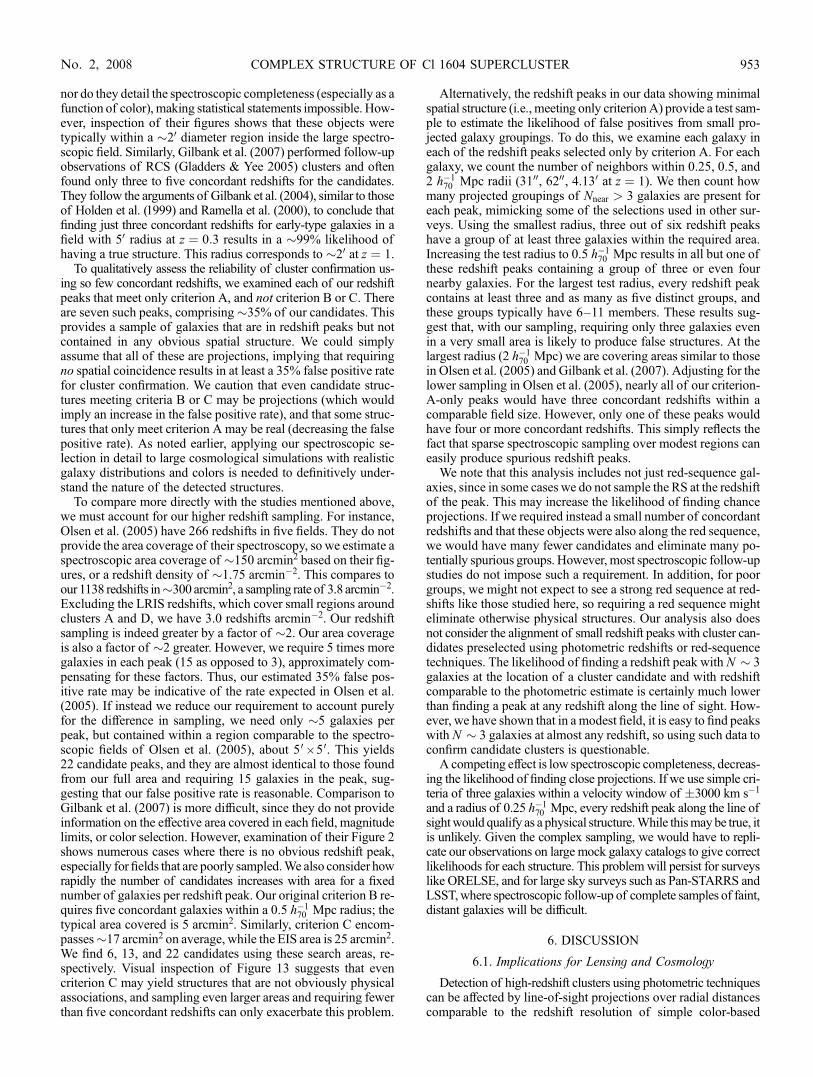
nor do they detail the spectroscopic completeness (especially as afunction of color), making statistical statements impossible. How-ever, inspection of their figures shows that these objects weretypically within a �20 diameter region inside the large spectro-scopic field. Similarly, Gilbank et al. (2007) performed follow-upobservations of RCS (Gladders & Yee 2005) clusters and oftenfound only three to five concordant redshifts for the candidates.They follow the arguments of Gilbank et al. (2004), similar to thoseof Holden et al. (1999) and Ramella et al. (2000), to conclude thatfinding just three concordant redshifts for early-type galaxies in afield with 50 radius at z ¼ 0:3 results in a �99% likelihood ofhaving a true structure. This radius corresponds to �20 at z ¼ 1.

To qualitatively assess the reliability of cluster confirmation us-ing so few concordant redshifts, we examined each of our redshiftpeaks that meet only criterion A, and not criterion B or C. Thereare seven such peaks, comprising�35% of our candidates. Thisprovides a sample of galaxies that are in redshift peaks but notcontained in any obvious spatial structure. We could simplyassume that all of these are projections, implying that requiringno spatial coincidence results in at least a 35% false positive ratefor cluster confirmation. We caution that even candidate struc-tures meeting criteria B or C may be projections (which wouldimply an increase in the false positive rate), and that some struc-tures that only meet criterion A may be real (decreasing the falsepositive rate). As noted earlier, applying our spectroscopic se-lection in detail to large cosmological simulations with realisticgalaxy distributions and colors is needed to definitively under-stand the nature of the detected structures.

To compare more directly with the studies mentioned above,we must account for our higher redshift sampling. For instance,Olsen et al. (2005) have 266 redshifts in five fields. They do notprovide the area coverage of their spectroscopy, so we estimate aspectroscopic area coverage of �150 arcmin2 based on their fig-ures, or a redshift density of �1.75 arcmin�2. This compares toour 1138 redshifts in�300 arcmin2, a sampling rate of 3.8 arcmin�2.Excluding the LRIS redshifts, which cover small regions aroundclusters A and D, we have 3.0 redshifts arcmin�2. Our redshiftsampling is indeed greater by a factor of �2. Our area coverageis also a factor of �2 greater. However, we require 5 times moregalaxies in each peak (15 as opposed to 3), approximately com-pensating for these factors. Thus, our estimated 35% false pos-itive rate may be indicative of the rate expected in Olsen et al.(2005). If instead we reduce our requirement to account purelyfor the difference in sampling, we need only �5 galaxies perpeak, but contained within a region comparable to the spectro-scopic fields of Olsen et al. (2005), about 50 ; 50. This yields22 candidate peaks, and they are almost identical to those foundfrom our full area and requiring 15 galaxies in the peak, sug-gesting that our false positive rate is reasonable. Comparison toGilbank et al. (2007) is more difficult, since they do not provideinformation on the effective area covered in each field, magnitudelimits, or color selection. However, examination of their Figure 2shows numerous cases where there is no obvious redshift peak,especially for fields that are poorly sampled.We also consider howrapidly the number of candidates increases with area for a fixednumber of galaxies per redshift peak. Our original criterion B re-quires five concordant galaxies within a 0.5 h�1

70 Mpc radius; thetypical area covered is 5 arcmin2. Similarly, criterion C encom-passes�17 arcmin2 on average, while the EIS area is 25 arcmin2.We find 6, 13, and 22 candidates using these search areas, re-spectively. Visual inspection of Figure 13 suggests that evencriterion C may yield structures that are not obviously physicalassociations, and sampling even larger areas and requiring fewerthan five concordant redshifts can only exacerbate this problem.

Alternatively, the redshift peaks in our data showing minimalspatial structure (i.e., meeting only criterion A) provide a test sam-ple to estimate the likelihood of false positives from small pro-jected galaxy groupings. To do this, we examine each galaxy ineach of the redshift peaks selected only by criterion A. For eachgalaxy, we count the number of neighbors within 0.25, 0.5, and2 h�1

70 Mpc radii (3100, 6200, 4.130 at z ¼ 1). We then count howmany projected groupings of Nnear > 3 galaxies are present foreach peak, mimicking some of the selections used in other sur-veys. Using the smallest radius, three out of six redshift peakshave a group of at least three galaxies within the required area.Increasing the test radius to 0.5 h�1

70 Mpc results in all but one ofthese redshift peaks containing a group of three or even fournearby galaxies. For the largest test radius, every redshift peakcontains at least three and as many as five distinct groups, andthese groups typically have 6Y11 members. These results sug-gest that, with our sampling, requiring only three galaxies evenin a very small area is likely to produce false structures. At thelargest radius (2 h�1

70 Mpc) we are covering areas similar to thosein Olsen et al. (2005) and Gilbank et al. (2007). Adjusting for thelower sampling in Olsen et al. (2005), nearly all of our criterion-A-only peaks would have three concordant redshifts within acomparable field size. However, only one of these peaks wouldhave four or more concordant redshifts. This simply reflects thefact that sparse spectroscopic sampling over modest regions caneasily produce spurious redshift peaks.

We note that this analysis includes not just red-sequence gal-axies, since in some cases we do not sample the RS at the redshiftof the peak. This may increase the likelihood of finding chanceprojections. If we required instead a small number of concordantredshifts and that these objects were also along the red sequence,we would have many fewer candidates and eliminate many po-tentially spurious groups. However, most spectroscopic follow-upstudies do not impose such a requirement. In addition, for poorgroups, we might not expect to see a strong red sequence at red-shifts like those studied here, so requiring a red sequence mighteliminate otherwise physical structures. Our analysis also doesnot consider the alignment of small redshift peaks with cluster can-didates preselected using photometric redshifts or red-sequencetechniques. The likelihood of finding a redshift peak with N � 3galaxies at the location of a cluster candidate and with redshiftcomparable to the photometric estimate is certainly much lowerthan finding a peak at any redshift along the line of sight. How-ever, we have shown that in a modest field, it is easy to find peakswith N � 3 galaxies at almost any redshift, so using such data toconfirm candidate clusters is questionable.

A competing effect is low spectroscopic completeness, decreas-ing the likelihood of finding close projections. If we use simple cri-teria of three galaxies within a velocity window of �3000 km s�1

and a radius of 0.25 h�170 Mpc, every redshift peak along the line of

sightwould qualify as a physical structure.While thismaybe true, itis unlikely. Given the complex sampling, we would have to repli-cate our observations on large mock galaxy catalogs to give correctlikelihoods for each structure. This problem will persist for surveyslike ORELSE, and for large sky surveys such as Pan-STARRS andLSST,where spectroscopic follow-up of complete samples of faint,distant galaxies will be difficult.

6. DISCUSSION

6.1. Implications for Lensing and Cosmology

Detection of high-redshift clusters using photometric techniquescan be affected by line-of-sight projections over radial distancescomparable to the redshift resolution of simple color-based


techniques. Cohn et al. (2007) show that many clusters detectedin a red-sequence type survey at z � 1 are made up of galaxiesfrom multiple distinct cluster-size dark matter halos. Their workdoes not include smaller groups, of which we expect to findmany in the infall regions of high-redshift clusters. They alsodemonstrate that the problem becomes substantially worse atz � 1 than it is at z � 0:5, in part because a fixed pair of filterscannot sample features such as the 4000 8 break over such abroad redshift range.

We find many small groups in both the foreground and back-ground of the target structure at z � 0:9. Examination of modelgalaxy tracks fromBruzual &Charlot (2003) in the r 0 � i0 versusi0 � z0 color-color space for both galaxies with a single burst atz ¼ 3 and the RCSmodel (a 0.1 Gyr burst ending at z ¼ 2:5 witha � ¼ 0:1 Gyr exponential decline thereafter) shows that colorsfor galaxies over a moderately broad redshift range (z � 0:8Y1:2) are quite similar, with the differences in color comparable toground-based photometric errors (ORELSE I). Therefore, anysurvey relying on only two- or three-color moderate-depth ground-based imaging is subject to this type of confusion. The surveys willbe biased toward detecting projected systems, the same problemthat has plagued lower redshift optical cluster catalogs (Katgertet al.1996). Even with large cosmological simulations, the detailedeffects of such projections on cluster detection, number counts, andmass estimates will be difficult to quantify. The most recent studies(Cohn et al. 2007 ) using the Millennium Simulation and a red-sequence cluster finder are still hampered by the inability of simula-tions to reproduce the observed colors of cluster galaxies. Extensivespectroscopy of at least a subset of clusters found using optical andX-ray surveys is needed to understand the contamination rates,redshift distributions, substructure, and other cluster properties;such work is only now under way (Gilbank et al. 2007).

Given that such projections can only enhance the detectabilityof lowermass systems, as well as inflate velocity dispersions andincrease the weak-lensing signal, mass estimates for single boundcluster components using such techniques will always tend to beoverestimated. A striking example is Cluster A (Cl 1604+4304),whose initial velocity dispersion estimate was 1200 km s�1

(Postman et al. 2001). Adding many more spectra, but nottightly restricting the area sampled, Gal & Lubin (2004) found� ¼ 700 km s�1. We now find that the velocity dispersion can beas low as � ¼ 532 km s�1, more than a factor of 2 below theinitial measurement. Comparison of velocity dispersions derivedusing a variety of galaxy subpopulations (as done in x 4.1.3) withsimulations is necessary to determine the optimal mass tracer.

Hoekstra (2003) suggested that structures associated with, butnot bound to, a cluster can increase errors in lensing mass estimatestwofold. Our data show that such filaments may be common atz � 1. Furthermore, completely independent structures along theline of sight can be cause for concern, even at low redshift (xokaset al. 2006). In Cl 1604, we find moderate-mass groups at z � 1:2directly projected onto clusters at z � 0:9. Both types of structurescan affect the derived mass profiles. Typically, NFW profiles(Navarro et al. 1996) are fitted to clusters in both observationsand simulations; clusters have been observed with NFW concen-trations c incompatible with simulated clusters. Very recent sim-ulations of weak lensing by clusters plus foreground group-sizehalos (King & Corless 2007) demonstrate that line-of-sight con-tamination by even low-mass systems can both decrease andincrease the measured value of c, depending on the geometry. Itis not yet known howmuch this can affect the overall distributionof observed concentrations and masses from weak lensing. Im-plementing techniques that incorporate multiwavelength data(X-ray, Sunyaev-Zel’dovich, optical) can overcome some of

these issues but requires both extensive data and computationalpower (Mahdavi et al. 2007), limiting it to rich, low-redshift clus-ters or only the most massive structures at higher redshift for thetime being. With somewhat less data, it is possible to compareX-ray and weak-lensing masses for clusters. Recent work usingobservational data has shown moderate agreement between thesetwo techniques, but discrepancies are plentiful and systematicerrors are much too large for precision cosmological measure-ments (Sehgal et al. 2008). In contrast, some lensing simulationsclaim that high completeness, low contamination, and goodmassfidelity can be achieved with weak lensing (Pace et al. 2007), butthis has yet to be proven with large samples of real data.Weak lensing has already been used to estimate the mass of

Cl 1604+4304 (cluster A; Margoniner et al. 2005), resulting in amass of (3:67 � 1:47)(R/500 kpc) ; 1014 M�, corresponding toa velocity dispersion of 1009 � 199 km s�1. This is significantlyhigher than the 575þ110

�85 km s�1 estimated from the cluster’sX-ray temperature of TX ¼ 2:51þ1:05

�0:69 keV (Lubin et al. 2004).The velocity dispersion presented here lies in between these twoestimates but is much more consistent with the X-ray tempera-ture. Earlier work on a much smaller region using HST WFPC2data suggestedmultiplemass peaks associated with this structure(Umetsu & Futamase 2000). Cl 1604+4304 is the most isolatedcomponent of the supercluster, with the only foreground struc-tures being a group at z ¼ 0:495 and a possible wall at z ¼ 0:600.Nevertheless, its estimated mass varies by a factor of nearly 2.ImprovedX-raymeasurements from deepChandra observations(Kocevski et al. 2008) and lensing data from a recent ACSmosaic,combined with our spectroscopic database, may help resolve thisdiscrepancy.Instead of measuring individual cluster masses, one could avoid

some of the above problems with a sufficiently large and deepsurvey by calculating the mass on very large (�100 Mpc) scalesover several superclusters and comparing the results to simu-lations and structure formation theories, but such surveys remainin the future.With excellent deep photometric data, it is also pos-sible to use weak-lensing tomography, incorporating photometricredshifts to map all the galaxies along the line of sight. However,even the best photometric redshifts have errors that are equal to orgreater than the entire redshift depth of the Cl 1604 structure(Margoniner & Wittman 2008). As a result, uncertainties in thebias and scatter of photo-z estimators with redshift remain a prob-lem (Ma et al. 2006) and will require extensive spectroscopy tocalibrate.Finally, we note that Cl 1604 is an optically selected large-

scale structure. To whatever extent it is not representative of allstructures at similar redshifts, any conclusions based on Cl 1604alone may be biased. For this reason, the ORELSE survey hasincluded a variety of structures originally detected using X-ray,optical, and even radio techniques. Once the survey is complete,we can address biases due to the cluster detection technique.Within Cl 1604, the supercluster members were targeted basedon their red colors (see x 3), so that the blue galaxy populationmay be undersampled; nevertheless, �50% of the targets areoutside the red sequence.

6.2. Future Work

The extensive spectroscopic database described here is beingused for a variety of projects. Detailed analysis of line strengthsas a function of position in the structure, local density, and hostcluster properties is being derived by stacking spectra (B. C.Lemaux et al. 2008a, in preparation). The redshift range of thesupercluster along with our spectral setup forces the use of the[O ii] doublet at 3727 8 as a proxy for H� emission and thus


ongoing star formation activity. Since [O ii] has been shown to bea flawed tracer (Yan et al. 2006), we are using near-IR spectro-scopy to search for H� emission in a subset of our confirmedsupercluster members in order to determine the contribution ofnonstellar (i.e., nuclear) sources to the observed [O ii] emission.We have also serendipitously detected a significant number ofz > 4 Ly� sources in the DEIMOS data, and their properties willbe described in B. C. Lemaux et al. (2008b, in preparation).

A 17-pointing ACS mosaic of the field is being used to ex-amine the CMDs of individual clusters, in the manner of Homeieret al. (2006) and Andreon (2008), who used two earlier pointingscentered on clusters A andD. These images also allow us to com-pare galaxy colors and morphologies with their spectroscopicproperties and relate them to their location within the superclu-ster. Deep Chandra observations are being used to map the dis-tribution of active galactic nuclei (AGNs) within the superclusterand determine the X-ray luminosity (and hence mass) of indi-vidual clusters in the complex (Kocevski et al. 2008). Our spec-troscopic database, along with our ACS imaging, will allow us toexamine the spectral and morphological properties of AGN hostgalaxies, as well as their local environments, in order to shed lighton the mechanisms that trigger nuclear activity in these systems.DeepVLA1.4GHzmapping of the field shows both bright AGN-like sources and an excess of faint, possibly starbursting galaxies(N. Miller et al. 2008, in preparation). Preliminary results alreadysuggest signs of environmental segregation, with the radio-loudpopulation found in dense regions that the radio-faint and X-rayYdetected AGNs avoid.

Deep Spitzer IRAC and MIPS maps have been obtained, pro-viding both rest-frameK-band luminosities to estimate the stellarmass content of member galaxies and infrared fluxes to searchfor obscured star formation that is more prevalent at higher red-shifts. Ground-based K-band imaging is also being used for stel-lar mass estimation. Combining all of these observations willallow detailed SED fitting and modeling of the star formationhistories of supercluster members. For galaxies without spectro-scopy, the extensive multiwavelength data will be used to esti-mate redshifts photometrically, both as input to lensing modelsand to better map the supercluster structure.

7. CONCLUSIONS

We have presented the results of an extensive spectroscopiccampaign to map the Cl 1604 supercluster at z � 0:9. With over400 confirmed members, this database provides coverage com-parable to studies of local structures, but at a look-back time of7 Gyr. The large number of redshifts is crucial for confirming theindividual clusters, measuring accurate velocity dispersions, andfinding contamination due to foreground and background clusters.A three-dimensional map of the supercluster is constructed, mak-ing possible the comparison of such structures to large simu-lations.We also report the discovery of a poor cluster at z ¼ 1:207with at least 15 confirmed members within a �600 km s�1 win-dow and 1 h�1

70 Mpc radius, making it one of the highest redshiftstructures selected spectroscopically.

This data set forms the foundation for a variety of follow-up stud-ies, usingmanywavelengths to identify preferred sites for inducingand quenching star formation and AGN activity. The extensivespectroscopy allows identification of samples of rare objects,including radio and X-ray sources within the supercluster. With-out the large number of redshifts, it is impossible to definitivelyassociate individual objects with the supercluster due to themany sources along the line of sight that are not physically as-sociated with the structure. As an example, Kocevski et al. (2008)and N. Miller et al. (2008, in preparation) show that X-ray and

radio sources within the supercluster are a very small fractionof the total number of such sources in the field. The same is truefor infrared sources such as starbursts. Construction of lumi-nosity functions for these rarer sources has traditionally beenhampered by the lack of redshifts (Branchesi et al. 2006); oursurvey is designed to alleviate these problems. The only compar-able project is the PISCES program, with deep optical imagingand spectroscopy of high-z clusters with Subaru, but their targetsare typically more massive clusters and their spectroscopic fol-low-up is much less complete. Field surveys such as GOODS,AEGIS, and COSMOS provide similar data to ORELSE, in termsof both multiwavelength and spectroscopic coverage, but lackthe sampling of dense environments. For instance, COSMOScontains just one large-scale structure at z � 0:7 (Guzzo et al.2007).

Such detailed mapping, encompassing large (>10Mpc) areas,will be essential for a statistical sample of clusters over a wideredshift baseline to understand the diversity of structures theyare embedded in. The redshift depth of the supercluster is com-parable to photometric redshift errors achievable from opticalground-based surveys, and especially two-band cluster surveys,potentially enhancing its detectability. At such high redshifts,photometric errors are larger for faint galaxies, photometric red-shift errors increase, the change in color of the red sequence withunit �z is reduced (see Fig. 1 of Gladders & Yee 2005), andclusters are still in the process of merging and accreting theirgalaxies. All of these effects complicate our ability to reliablyconstruct cluster catalogs over a wide range of redshifts. Futureprograms relying on photometric redshifts, weak lensing, S-Z,and X-ray data (in particular, luminosities) to estimate clustermasses must understand the biases inherent in each technique,especially when using large samples to constrain cosmologicalparameters. While large cosmological simulations can provideinsight into these issues, their current inability to accurately re-produce galaxy properties, especially colors, means that moreobservations are necessary. The ORELSE survey will providesuch data on a variety of structures at 0:6 < z < 1:2, forming aninvaluable resource for both galaxy evolution and cosmologicalstudies.

Thismaterial is based onwork supported by the National Aero-nautics and Space Administration under award NNG05GC34ZGfor the Long Term Space Astrophysics Program. Support forprogram HST-GO-08560.05-Awas provided by NASA througha grant from the Space Telescope Science Institute, which isoperated by the Association of Universities for Research in As-tronomy, Inc., under NASA contract NAS 5-26555. The spectro-graphic data presented herein were obtained at the W. M. KeckObservatory, which is operated as a scientific partnership amongthe California Institute of Technology, the University of Cal-ifornia, and the National Aeronautics and Space Administration.The Observatory was made possible by the generous financialsupport of the W. M. Keck Foundation. The authors wish torecognize and acknowledge the very significant cultural role andreverence that the summit of Mauna Kea has always had withinthe indigenous Hawaiian community. We are most fortunate tohave the opportunity to conduct observations from this moun-tain. The observing staff, telescope operators, and instrumentscientists at Keck provided a great deal of assistance. We wouldalso like to thank the DEEP2 team for making their softwareavailable to us, and especially M. Cooper for his assistance withimplementation.


REFERENCES

Adelman-McCarthy, J. K., et al. 2008, ApJS, 175, 297Andreon, S. 2008, MNRAS, 386, 1045Beers, T. C., Flynn, K., & Gebhardt, K. 1990, AJ, 100, 32Bertin, E., & Arnouts, S. 1996, A&AS, 117, 393Bower, R. G., Lucey, J. R., & Ellis, R. S. 1992, MNRAS, 254, 589Branchesi, M., Gioia, I. M., Fanti, C., Fanti, R., & Perley, R. 2006, A&A, 446,97

Bruzual, G., & Charlot, S. 2003, MNRAS, 344, 1000Cohn, J. D., Evrard, A. E., White, M., Croton, D., & Ellingson, E. 2007,MNRAS, 382, 1738

Cooper, M. C. 2007, Ph.D. thesis, Univ. California, BerkeleyDavis, M., et al. 2003, Proc. SPIE, 4834, 161De Filippis, E., Sereno, M., Bautz, M. W., & Longo, G. 2005, ApJ, 625, 108Dressler, A. 1980, ApJ, 236, 351Dressler, A., & Shectman, S. A. 1988, AJ, 95, 985Faber, S. M., et al. 2003, Proc. SPIE, 4841, 1657Ford, H. C., et al. 2003, Proc. SPIE, 4854, 81Gal, R. R., de Carvalho, R. R., Lopes, P. A. A., Djorgovski, S. G., Brunner, R.J., Mahabal, A., & Odewahn, S. C. 2003, AJ, 125, 2064

Gal, R. R., & Lubin, L. M. 2004, ApJ, 607, L1Gal, R. R., Lubin, L. M., & Squires, G. K. 2005, AJ, 129, 1827Gilbank, D. G., Bower, R. G., Castander, F. J., & Ziegler, B. L. 2004, MNRAS,348, 551

Gilbank, D. G., Yee, H. K. C., Ellingson, E., Gladders, M. D., Barrientos, L. F.,& Blindert, K. 2007, AJ, 134, 282

Gilbank, D. G., Yee, H. K. C., Ellingson, E., Hicks, A. K., Gladders, M. D.,Barrientos, L. F., & Keeney, B. 2008, ApJ, 677, L89

Gladders, M. D., & Yee, H. K. C. 2000, AJ, 120, 2148———. 2005, ApJS, 157, 1Gunn, J. E., Hoessel, J. G., & Oke, J. B. 1986, ApJ, 306, 30Guzzo, L., et al. 2007, ApJS, 172, 254Hoekstra, H. 2003, MNRAS, 339, 1155Holden, B. P., Nichol, R. C., Romer, A. K., Metevier, A., Postman, M., Ulmer,M. P., & Lubin, L. M. 1999, AJ, 118, 2002

Homeier, N. L., et al. 2006, ApJ, 647, 256Jannuzi, B. T., & Dey, A. 1999, in ASP Conf. Ser. 191, Photometric Redshiftsand the Detection of High-Redshift Galaxies, ed. R. Weymann et al. (SanFrancisco: ASP), 111

Jing, Y. P., & Suto, Y. 2002, ApJ, 574, 538Katgert, P., et al. 1996, A&A, 310, 8Kells, W., Dressler, A., Sivaramakrishnan, A., Carr, D., Koch, E., Epps, H.,Hilyard, D., & Pardeilhan, G. 1998, PASP, 110, 1487

King, L., & Corless, V. 2007, MNRAS, 374, L37Kocevski, D., Lubin, L. M., Gal, R., Lemaux, B. C., Fassnacht, C. D., &Squires, G. K. 2008, preprint (arXiv:0804.1955)

Kodama, T., & Arimoto, N. 1997, A&A, 320, 41Kodama, T., et al. 2005, PASJ, 57, 309Lee, J., & Evrard, A. E. 2007, ApJ, 657, 30xokas, E. L., Prada, F., Wojtak, R., Moles, M., & Gottlober, S. 2006, MNRAS,366, L26

Lubin, L. M., Brunner, R., Metzger, M. R., Postman, M., & Oke, J. B. 2000,ApJ, 531, L5

Lubin, L. M., Mulchaey, J. S., & Postman, M. 2004, ApJ, 601, L9Lubin, L. M., Oke, J. B., & Postman, M. 2002, AJ, 124, 1905Lubin, L. M., Postman, M., Oke, J. B., Ratnatunga, K. U., Gunn, J. E., Hoessel,J. G., & Schneider, D. P. 1998, AJ, 116, 584

Ma, Z., Hu, W., & Huterer, D. 2006, ApJ, 636, 21Mahdavi, A., Hoekstra, H., Babul, A., Sievers, J., Myers, S. T., & Henry, J. P.2007, ApJ, 664, 162

Margoniner, V. E., Lubin, L. M., Wittman, D. M., & Squires, G. K. 2005, AJ,129, 20

Margoniner, V. E., & Wittman, D. M. 2008, ApJ, 679, 31McIntosh, D. H., Zabludoff, A. I., Rix, H.-W., & Caldwell, N. 2005, ApJ, 619,193

Mei, S., et al. 2006, ApJ, 639, 81Navarro, J. F., Frenk, C. S., & White, S. D. M. 1996, ApJ, 462, 563Nuijten, M. J. H. M., Simard, L., Gwyn, S., & Rottgering, H. J. A. 2005, ApJ,626, L77

Oke, J. B., Postman, M., & Lubin, L. M. 1998, AJ, 116, 549Oke, J. B., et al. 1995, PASP, 107, 375Olsen, L. F., Zucca, E., Bardelli, S., Benoist, C., da Costa, L., Jørgensen, H. E.,Biviano, A., & Ramella, M. 2005, A&A, 442, 841

Pace, F., Maturi, M., Meneghetti, M., Bartelmann, M., Moscardini, L., &Dolag, K. 2007, A&A, 471, 731

Paz, D. J., Lambas, D. G., Padilla, N., & Merchan, M. 2006, MNRAS, 366,1503

Pinkney, J., Roettiger, K., Burns, J. O., & Bird, C. M. 1996, ApJS, 104, 1Plionis, M., Basilakos, S., & Ragone-Figueroa, C. 2006, ApJ, 650, 770Postman, M., Lubin, L. M., Gunn, J. E., Oke, J. B., Hoessel, J. G., Schneider,D. P., & Christensen, J. A. 1996, AJ, 111, 615

Postman, M., Lubin, L. M., & Oke, J. B. 1998, AJ, 116, 560———. 2001, AJ, 122, 1125Ramella, M., et al. 2000, A&A, 360, 861Schlegel, D. J., Finkbeiner, D. P., & Davis, M. 1998, ApJ, 500, 525Scoville, N., et al. 2007, ApJS, 172, 150Sehgal, N., Hughes, J. P., Wittman, D., Margoniner, V., Tyson, J. A., Gee, P., &dell’Antonio, I. 2008, ApJ, 673, 163

Sereno, M., De Filippis, E., Longo, G., & Bautz, M. W. 2006, ApJ, 645, 170Simcoe, R. A., Metzger, M. R., Small, T. A., & Araya, G. 2000, BAAS, 32, 758Small, T. A., Ma, C.-P., Sargent, W. L. W., & Hamilton, D. 1998, ApJ, 492, 45Smith, G. P., Treu, T., Ellis, R. S., Moran, S. M., & Dressler, A. 2005, ApJ, 620, 78Swinbank, A. M., et al. 2007, MNRAS, 379, 1343Tanaka, M., Goto, T., Okamura, S., Shimasaku, K., & Brinkmann, J. 2004, AJ,128, 2677

Umetsu, K., & Futamase, T. 2000, ApJ, 539, L5Visvanathan, N., & Sandage, A. 1977, ApJ, 216, 214Yan, R., Newman, J. A., Faber, S. M., Konidaris, N., Koo, D., & Davis, M.2006, ApJ, 648, 281

York, D. G., et al. 2000, AJ, 120, 1579Zabludoff, A. I., & Franx, M. 1993, AJ, 106, 1314

GAL ET AL.956

the complex structure of the cl 1604 …authors.library.caltech.edu/11833/1/galapj08.pdfthe complex...

Documents