the choking index: an analysis of … · the choking index: an analysis of performance under...
TRANSCRIPT

THE CHOKING INDEX: AN ANALYSIS OF PERFORMANCE UNDER PRESSURE ON THE PGA TOUR
By
SAMMI SMITH
A SENIOR RESEARCH PROPOSAL PRESENTED TO THE DEPARTMENT OF MATHEMATICS AND COMPUTER SCIENCE OF STETSON UNIVERSITY IN PARTIAL
FULFILLMENT OF THE REQUIREMENTS FOR THE DEGREE OF BACHELOR OF SCIENCE
STETSON UNIVERSITY
2013

2
ACKNOWLEDGMENTS
First and foremost, I would like to thank my advisor, Dr. William Miles, for all the
support and encouragement that he has given me in my three years at Stetson so far. From the
outstanding explanations of concepts in class lectures, to the willingness to go out of his way to
meet with me to help with a concept that I was struggling with, to the support he has shown me as
a student-athlete by coming to watch me play at tournaments, I am sure that my college
experience would not have been as wonderful as it has been so far had he not been a part of it. To
both Dr. Miles and his wife, Andi, thank you for always encouraging me and simply making my
day brighter with your smiles and sense of humor. Last but certainly not least, thank you for
allowing me to get to know your daughter. Emmy is lucky to have such wonderful parents.
Next, I would like to thank the other faculty and staff in the Math and CS department.
This department truly cares about its students and I can honestly say that each faculty member
who I have interacted with clearly wants, above all, for their students to learn and grow as
scholars and as people. To Nancy Wilton, thanks for always making me laugh and providing me
some occasional much-needed distraction from schoolwork. This department has made me feel at
home at Stetson, even though I was 1000 miles away from home. I cannot thank you guys
enough for that.
Also, on a note more specific to this project, thank you to Dr. Camille King for her
assistance in helping me understand the psychological aspects of pressure and sports.
I am very grateful for my family, especially my parents, and my friends who always
believed in me and pushed me to become a better person, a better student, and a better athlete.
Without their constant support, I don’t know how I would have survived the challenges of
college.
Finally, I would like to thank the Edmunds family for giving me the opportunity to attend
such an amazing academic institution. Without their financial support, there is no way I would be
able to be here today.
3
TABLE OF CONTENTS
ACKNOWLEDGEMENTS ---------------------------------------------------------------------------- 2 LIST OF TABLES -------------------------------------------------------------------------------------- 5 LIST OF FIGURES ------------------------------------------------------------------------------------- 6 ABSTRACT --------------------------------------------------------------------------------------------- 7 CHAPTERS 1. INTRODUCTION ---------------------------------------------------------------------------------
1.1. Background and Objective ------------------------------------------------------------------ 1.2. Description Of Choke And Clutch --------------------------------------------------------- 1.3. Cause Of Choking Under Pressure --------------------------------------------------------- 1.4. Findings From Other Sports ---------------------------------------------------------------- 1.5. The Basics of a Round of Golf ------------------------------------------------------------- 1.6. Data Source ------------------------------------------------------------------------------------
8 8 8 8 9
10 11
2. PRESSURE SCENARIOS ------------------------------------------------------------------------ 2.1. Situations In Which A Player Would Feel Pressure ------------------------------------- 2.2. Player Performance In The Last Round --------------------------------------------------- 2.3. Player Performance In The Last Round When In Contention --------------------------
2.3.1. Defining “In Contention” ----------------------------------------------------------
11 11 12 14 14
3. ATTEMPTED APPROACHES ------------------------------------------------------------------ 3.1. Choking Function ----------------------------------------------------------------------------
3.1.1. Single Variable Function ---------------------------------------------------------- 3.1.2. Multivariable Function ------------------------------------------------------------- 3.1.3. Correlation ---------------------------------------------------------------------------
3.2. Choking Index --------------------------------------------------------------------------------
17 17 17 20 20 21
4. STATISTICAL ANALYSIS ---------------------------------------------------------------------- 4.1. Overview --------------------------------------------------------------------------------------- 4.2. Delta Score For A Player In The Lead ----------------------------------------------------- 4.2.1. Attempts To Handle The Leader Exception ------------------------------------- 4.2.2. Simplified Handling Of The Leader Exception --------------------------------- 4.3. Performance In The Last Round ------------------------------------------------------------ 4.3.1. Choice For Level Of Significance ------------------------------------------------ 4.3.2. Scale That Ranks Players Relative To Each Other ----------------------------- 4.3.3. Explanation Of The Process With An Example -------------------------------- 4.3.4. Best And Worst Ranked Players -------------------------------------------------- 4.4. Performance In The Last Round When In Contention ----------------------------------- 4.4.1. Student’s T Test For Initial Testing ---------------------------------------------- 4.4.2. Recasting The Population Definition --------------------------------------------- 4.4.3. Finding An Suitable Test ----------------------------------------------------------- 4.4.4. Description Of Welch’s T Test ---------------------------------------------------- 4.4.5. Results Of Welch’s T Test --------------------------------------------------------- 4.4.6. Welch’s T Test Relative To The Field ------------------------------------------- 4.4.7. Scale That Ranks Players Relative To Each Other ----------------------------- 4.4.8. Explanation Of The Process With An Example -------------------------------- 4.4.9. Best And Worst Ranked Players -------------------------------------------------- 4.4.10. Welch’s T Test Using Fourth Round Relative To The Field ----------------- 4.5. Conclusion ------------------------------------------------------------------------------------
21 21 21 23 25 26 27 28 29 29 30 31 32 32 34 34 37 38 38 40 40 42
5. PROPOSED FUTURE RESEARCH IDEAS --------------------------------------------------- 5.1. Choking Index For Players Near The Cut Line -------------------------------------------
42 42

4
5.2. Testing The Normally Distributed Populations Assumption --------------------------- 5.3. Specific Part Of The Game ------------------------------------------------------------------ 5.4. Parameterized Model ------------------------------------------------------------------------- 5.5. Intimidation Index ----------------------------------------------------------------------------
43 43 44 45
APPENDIX ---------------------------------------------------------------------------------------------- 46 REFERENCES ------------------------------------------------------------------------------------------ 55
5
LIST OF TABLES
TABLE
1. Best Ten and Worst Ten Choking Indices: Performance in the Last Round ---------------- 2. Best Ten and Worst Ten Choking Indices: Performance in the Last Round In
Contention, Δ Score --------------------------------------------------------------------------------- 3. Best Ten and Worst Ten Choking Indices: Performance in the Last Round In
Contention, Fourth Round -------------------------------------------------------------------------- 4. All Three Choking Indices For All Players: Sorted By CIIC Δ score------------------------------
29
40
41 46
6
LIST OF FIGURES
FIGURE
1. Number of Strokes the Winner Was Behind After 54 Holes ---------------------------------- 2. Example Plots of Linear Regressions of Position vs. Δ Score for a Particular Player ----- 3. Scatterplot of Δ Score vs. Δ Position for All Golfers With Leaders Emphasized ---------- 4. Scatterplot of Δ Score vs. Δ Position for All Golfers Not In the Lead After Both Rounds
3 and 4 ------------------------------------------------------------------------------------------------- 5. Histograms of In Contention and Out of Contention Δ Scores For All Players ------------- 6. Noncentral T Distributions ------------------------------------------------------------------------- 7. Illustration of the Yerkes-Dodson Law -----------------------------------------------------------
15 19 22
23 33 36 44

7
ABSTRACT
THE CHOKING INDEX: AN ANALYSIS OF PERFORMANCE UNDER PRESSURE ON THE PGA TOUR
By Sammi Smith
May 2013
Advisor: Dr. William Miles Department: Mathematics and Computer Science In nearly all sports, athletes are frequently placed in pressure-filled situations. The way
the athlete responds to that stress is a key determinant of whether the competition is won or lost.
As a result, athletes often gain a positive or negative reputation based on their past performances
in this type of situation. An athlete who handles the pressure well and who actually performs in a
manner that is better than his typical performance is cast as a clutch performer. One who lets the
pressure impact him in a negative way is referred to as a choker. In this paper, we wish to
examine this phenomenon in the sport of golf, specifically regarding the professional golfers on
the PGA Tour. There are three main pressure scenarios that we will consider: the pressure of the
last round of a tournament, the additional pressure of the last round of a tournament when in
contention, and the pressure of being near the cut line.
In an attempt to classify each golfer as a clutch performer or a choker, we considered
creating both a function and an index for each player. Upon examining the advantages and
disadvantages of each, we determined that the index approach was best. Three choking indices
were created for each player, one that details a golfer’s tendency in the last round of a tournament
and two that detail a golfer’s tendency when in contention going into the last round of a
tournament. A choking index that describes a player’s performance near the cut line was left for
future consideration. All three indices were generated using various types of hypothesis testing.
Proposals for additional future work are also included.

8
CHAPTER 1
INTRODUCTION
1.1. BACKGROUND AND OBJECTIVE
The PGA (Professional Golf Association) Tour, the premier men’s professional golf tour
in the world, keeps a multitude of statistics on each of its members, regarding information such as
scoring average, driving distance, number of greens hit in regulation and number of putts per
round. However, these statistics mentioned barely scratch the surface of all the statistics kept by
the tour. Tour officials are forever searching for new ways to assess a player’s performance. We
propose to create a new statistic that measures how well a player performs in a high-pressure
situation compared to how well he performs in a typical situation.
1.2. DESCRIPTION OF CHOKE AND CLUTCH
Pressure can be defined as “any factor or combination of factors that increases the
importance of performing well” [1]. For any athlete, performance under pressure is a supremely
critical consideration. In nearly all sports, the game is won or lost based on the performance of
the athlete(s) when everything is on the line. With this in mind, athletes are frequently classified
based on how they perform in these pressure-filled situations. When an athlete performs very
well and exceeds expectations, he is often referred to as a “clutch” player. In contrast, when an
athlete does not live up to the expectations and performs poorly, he is typically cast as a
“choker”[2].
1.3. CAUSE OF CHOKING UNDER PRESSURE
University of Chicago psychologist Sian Beilock describes the phenomenon of choking
as “…suboptimal performance, not just poor performance. It’s a performance that is inferior to
what you can do and have done in the past and occurs when you feel pressure to get everything
right” [3]. Beilock’s research suggests that the predominant cause of choking is overthinking.
9
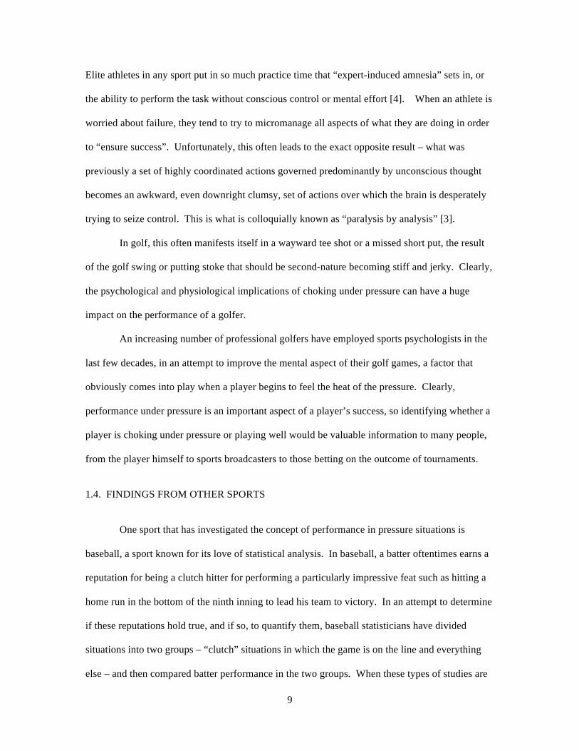
Elite athletes in any sport put in so much practice time that “expert-induced amnesia” sets in, or
the ability to perform the task without conscious control or mental effort [4]. When an athlete is
worried about failure, they tend to try to micromanage all aspects of what they are doing in order
to “ensure success”. Unfortunately, this often leads to the exact opposite result – what was
previously a set of highly coordinated actions governed predominantly by unconscious thought
becomes an awkward, even downright clumsy, set of actions over which the brain is desperately
trying to seize control. This is what is colloquially known as “paralysis by analysis” [3].
In golf, this often manifests itself in a wayward tee shot or a missed short put, the result
of the golf swing or putting stoke that should be second-nature becoming stiff and jerky. Clearly,
the psychological and physiological implications of choking under pressure can have a huge
impact on the performance of a golfer.
An increasing number of professional golfers have employed sports psychologists in the
last few decades, in an attempt to improve the mental aspect of their golf games, a factor that
obviously comes into play when a player begins to feel the heat of the pressure. Clearly,
performance under pressure is an important aspect of a player’s success, so identifying whether a
player is choking under pressure or playing well would be valuable information to many people,
from the player himself to sports broadcasters to those betting on the outcome of tournaments.
1.4. FINDINGS FROM OTHER SPORTS
One sport that has investigated the concept of performance in pressure situations is
baseball, a sport known for its love of statistical analysis. In baseball, a batter oftentimes earns a
reputation for being a clutch hitter for performing a particularly impressive feat such as hitting a
home run in the bottom of the ninth inning to lead his team to victory. In an attempt to determine
if these reputations hold true, and if so, to quantify them, baseball statisticians have divided
situations into two groups – “clutch” situations in which the game is on the line and everything
else – and then compared batter performance in the two groups. When these types of studies are

10
repeated by different scientists using various ways of grouping the clutch situations and various
ways to measure batter performance, the conclusion is almost always the same: a true clutch hitter
does not exist. In other words, a batter who was a good clutch hitter in one year was not
necessarily a good clutch hitter in subsequent years. [5]
Essentially, we wish to perform a similar type of analysis for golf, using the data from the
PGA Tour. It remains to be seen whether true clutch golfers or choke golfers exist. Since our
initial analysis thus far has considered only data from two years, it is possible that, like baseball, a
golfer with a tendency to choke (or be clutch) in one time period will not be any more likely to
choke (or be clutch) in another time period. However, we suspect that with golf this is not the
case. Once the analysis is extended to include more years in the data range, this claim can be
adequately verified or negated. Even if the data indicates that players are not consistent chokers
or clutch players over longer time periods, our analysis would still be useful because it would
indicate their most recent tendencies.
1.5. THE BASICS OF A ROUND OF GOLF
A round of golf consists of 18 holes, in which each hole is given a certain expected score,
known as par. Typically, each hole is either a par three, four, or five, where the par for the hole
specifies the score that an expert golfer should score on the hole. The sum of the pars for each
hole is known as the par for the course; this is usually 72. A PGA Tour tournament consists of
four rounds of golf on the course on separate days. There is almost always a cut after the second
day, in which the field is reduced based on the scores of each player in the first two rounds.
Usually, the top seventy players and ties make the cut, although some tournaments have slightly
different procedures for making the cut.

11
1.6. DATA SOURCE
In order to obtain data for research, we contacted the PGA Tour and were granted access
to the database of ShotLink, the company that keeps track of all data for the PGA Tour [6].
Initially, we have used data from all tournaments from the years 2011 and 2012. For our analysis,
data from those tournaments that are match play (in which the stroke score is not kept), rather
than stroke play, was thrown out. In addition, those tournaments that do not have a cut were
thrown out as well.
CHAPTER 2
PRESSURE SCENARIOS
2.1. SITUATIONS IN WHICH A PLAYER WOULD FEEL PRESSURE
There are several situations in which a player would feel a level of pressure that is greater
than normal. Some players have a reputation for playing well on Sunday, the final day of most
tournaments, while others have a tendency to play worse than usual on the last day. So, for the
players in the latter category, the last round is a pressure situation in which they do not perform
well. Similarly, certain players are known to struggle when they are close to the lead going into
the last day, while others tend to play better in that situation. Thus, being in contention on the last
day is a pressure situation, as well. Finally, most tournaments have a cut after two days of play,
in which the field is reduced. So, if a player did not play very well on the first day and is near the
cut line going into the second day, that is another type of pressure situation. It is likely that some
players will feel more pressure in one scenario and less in another.
While determining how much pressure a player actually “feels” would be rather difficult
to quantify, we can determine how a player reacts to the pressure situation by examining how
they perform.
Thus far, we have focused on performance on Sunday and performance when a player is
in contention on Sunday.

12
2.2. PLAYER PERFORMANCE IN THE LAST ROUND
First, we set out to determine how players react to the pressure of the last round. Initially,
we just compared scoring averages for a player’s first three rounds to their last round scoring
average, but upon further consideration, we decided that this was an unfair comparison. For each
round of a golf tournament, the course is set up differently, with tees in different areas and the
pins placed in different spots on the green. Clearly, some course setups can be much more
difficult than others. Typically, the course setups on the final day are designed to be the toughest,
in order to truly separate the best golfer from the rest of the field. In addition, some rounds are
more difficult than others due to circumstances beyond the tournament organizers’ control, such
as weather. Undoubtedly, a round played on a day with severe rain and wind will prove to be
much more difficult than a round played on a day that is sunny and calm. Therefore, each round
has an inherently different level of difficulty than the other rounds, so it is unfair to simply
compare a player’s scoring average for the first three rounds to that of the last round.
In order to take these considerations into account, we considered all scores relative to the
field’s mean score. The field’s mean score for a particular round at each tournament will indicate
the difficulty of the conditions, including course setup, weather, and any other factors that affect
the difficulty of play for that day. Thus, we can consider the field’s scoring average for a
particular round to be the “expected score” for an individual player for that round. If we subtract
this field mean score from the score of a particular player, we obtain a deviation from what was
expected. We will call this value the score relative to the field.
Therefore, for each player in each tournament, we need to determine the first three rounds
relative to the field and the last round relative to the field. Since we are mainly interested in
determining if a player plays significantly better or worse on the last day, we can group the first
three rounds together (by looking at the average of the first three rounds), rather than considering

13
each of the three separately. This gives the following two simple equations, where ! denotes
player, ! denotes field, and !"# denotes relative to the field:
3 !"#$% !"#$%&#!"# = 3 !"#$% !"#$%&# ! − 3 !"#$% !"#$%&#!
!"#$% !"#$%!"# = !"#$% !"#$% !"#$% ! − !"#$% !"#$% !"#$%! .
Next we look at the difference in these two computed values to determine if a player kept
up the scoring pace that he established in the first three rounds, or if he deviated significantly in
either direction. We will call this difference ∆ !"#$% and compute it as:
∆ !"#$% = !"#$% !"#$%!"# − 3 !"#$% !"#$%&#!"#.
Then, a ∆ !"#$% > 0 indicates a worse than expected performance or a “choke”, a
∆ !"#$% < 0 indicates a better than expected performance or a “clutch performance” and a
∆ !"#$% = 0 indicates that the player performed as expected.
Again, this type of statistic only measures how a player’s score changes relative to their
scores for the previous three days. Thus, it allows us to clearly see how a player reacts to the
pressure that is associated with the last day in any tournament.
If we group together for a particular player the values of ∆ !"#$% for each tournament,
then we can find the mean ∆ !"#$% for each player, call it !∆ !"#$%. We can then perform a
hypothesis test for each player with null hypothesis that !∆ !"#$% = 0 and alternative hypothesis
that !∆ !"#$% > 0 or !∆ !"#$% < 0 to determine if the player chokes or is clutch in the last round.

14
2.3. PLAYER PERFORMANCE IN THE LAST ROUND WHEN IN CONTENTION
In order to determine how a player reacts to the pressure of being in contention on the last
day, we can use our previous calculations, but take the analysis one step further. The additional
step consists of dividing each tournament in which each player competed into two categories.
One group includes all tournaments in which the player was in contention going into the last
round and the other group includes all tournaments in which the player was not in contention
going into the last round. Then, for each player, we determine the mean value for ∆ !"#$% when
he is in contention, and the mean value for ∆ !"#$% when he is out of contention, denoted as !!"
and !!" respectively. We will use these sample means, computed from a subset of all possible
scores consisting of all scores from the particular player for two years, to make decisions about
the true values of the population parameters !!" and !!" for each player.
If !!" > !!" , then the player has a tendency to choke under the pressure of being in
contention. If !!" < !!" , then the player has a tendency to turn in clutch performances. Clearly,
if !!" = !!" , then the player does not react to the pressure either positively or negatively.
Similarly, we can use the sample means !!" and !!" for the field (all players) to make
decisions about the true values of the population parameters !!" and !!" for the field. This will
tell us how the average golfer reacts to being in contention and will provide a useful metric with
which to compare the tendencies of individual players.
Finally, we can perform a hypothesis test to conclude whether or not these two values are
significantly different for each player, or significantly different for the field.
2.3.1. DEFINING “IN CONTENTION”
Although sportscasters frequently use the term “in-contention” to describe a player who
has a realistic chance of winning a tournament, this term has not been defined very clearly
anywhere. One of the first challenges of this project was delineating the cutoff point to define

15
whether a player is in contention or not. In-contention could be defined based on either the
number of strokes back or the number of positions back that a particular player is. We chose to
define it based on strokes because that is a more accurate measure of how far back from the lead a
player is and how difficult it would be to take over the lead.
For example, if going into the last round there are five players tied for second place one
shot back from the leader, then the next player, if he is one more shot back from the leader, would
be in seventh place. This player is only two shots back from the lead, but six positions back. So,
although he would have to pass six players to win the tournament, he only needs one stroke to
pass five of them and two strokes to pass them all. Thus, considering contention to be defined
based on score more accurately denotes a player’s proximity to the lead.
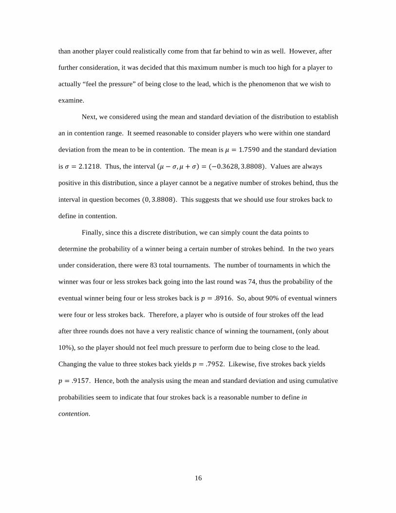
In order to establish an appropriate cutoff value that would place a player in contention or
not, we examined all tournaments in 2011 and 2012 to see how many strokes back after 54 holes,
or three rounds, each eventual winner was. As expected, these values had a decreasing
distribution.
Practically, this means that the majority of winners of tournaments were those who were
leading the tournament or within a few strokes of the leader after 54 holes. Initially, we
attempted to use the maximum number of strokes that any winner came from behind to win to
define in contention. In other words, if a player had won from that many strokes back before,
Winner: Number of Strokes Behind After 54 Holes
2 4 6 8
10
20
30
40
Figure 1. Number of Strokes the Winner Was Behind After 54 Holes.
16
than another player could realistically come from that far behind to win as well. However, after
further consideration, it was decided that this maximum number is much too high for a player to
actually “feel the pressure” of being close to the lead, which is the phenomenon that we wish to
examine.
Next, we considered using the mean and standard deviation of the distribution to establish
an in contention range. It seemed reasonable to consider players who were within one standard
deviation from the mean to be in contention. The mean is ! = 1.7590 and the standard deviation
is ! = 2.1218. Thus, the interval ! − !, ! + ! = (−0.3628, 3.8808). Values are always
positive in this distribution, since a player cannot be a negative number of strokes behind, thus the
interval in question becomes (0, 3.8808). This suggests that we should use four strokes back to
define in contention.
Finally, since this a discrete distribution, we can simply count the data points to
determine the probability of a winner being a certain number of strokes behind. In the two years
under consideration, there were 83 total tournaments. The number of tournaments in which the
winner was four or less strokes back going into the last round was 74, thus the probability of the
eventual winner being four or less strokes back is ! = .8916. So, about 90% of eventual winners
were four or less strokes back. Therefore, a player who is outside of four strokes off the lead
after three rounds does not have a very realistic chance of winning the tournament, (only about
10%), so the player should not feel much pressure to perform due to being close to the lead.
Changing the value to three stokes back yields ! = .7952. Likewise, five strokes back yields
! = .9157. Hence, both the analysis using the mean and standard deviation and using cumulative
probabilities seem to indicate that four strokes back is a reasonable number to define in
contention.

17
CHAPTER 3
ATTEMPTED APPROACHES
3.1. CHOKING FUNCTION
In addition to the index idea, we have also considered creating a “choking function” for
each player. Two approaches were attempted, both regression on a function of a single variable
and regression on a function of multiple variables. Both models used position after round three as
an independent variable. This type of approach has two clear advantages. First, it would allow us
to predict the outcome of a tournament based on the standings going into the last round. Second,
this would allow us to consider the tendency of a player to “choke” in the last round, no matter
what position they began the last round in. However, its disadvantage is, unlike the index
approach, we could not as concretely enumerate the tendencies of various players to choke under
pressure, so it would be more difficult to directly compare players with each other.
3.1.1. SINGLE VARIABLE FUNCTION
The first type of functional measure is a single variable choking function for each player
defining Δ !"#$% as a function of position after round three, regressing on data from the entire
range available. Each golfer would have one data point from each tournament, so we would
consider all tournaments in the entire year, or perhaps a two-year period, to create the function for
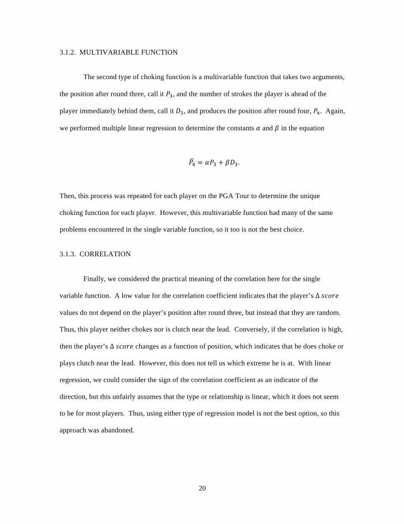
a particular player. However, when this was attempted on the data from 2011 and 2012, two
major problems were encountered. First, the majority of players did not have nearly enough data
points to lend confidence to the accuracy of the predictive value of our regression. Even if we
restricted our calculation to those players who had played in a certain minimum number of
tournaments, such as twenty, over the time period, the data points still did not range over the
possible positions nearly as much as we would like. For example, some players had many data
points with positions near the middle or bottom half of the field, but very few or none near the top

18
half. Thus, a regression model would lead to extrapolation if used to predict how a player would
finish when he is near the top of the leaderboard going into the last round. The other issue,
arguably a worse one, is that the data for most players did not seem to have any clear pattern.
Although it is not unreasonable to expect that some players would have a choking function with a
very different shape from other players, in order to create a regression model that accurately
predicts finishes, we would need for each player’s data set to have a clearly defined shape.
However, for most players who had a large number of data points that were spread across the
range of positions, we found that the plots of ∆ !"#$% as a function of position after round three
did not have a clearly defined pattern at all, whether it be linear, quadratic, exponential or any
other type of well-known shape. This reality was reflected in the low correlation coefficients
generated when the regression was performed.

19
0 10 20 30 40 50 60 70−10
−8
−6
−4
−2
0
2
4
6
8
10
position
delta
sco
re
Regression of Position vs Delta Score for a Particular Player
r =−0.84834
0 10 20 30 40 50 60 70−10
−8
−6
−4
−2
0
2
4
6
8
10
position
delta
sco
re
Regression of Position vs Delta Score for a Particular Player
r =1
0 10 20 30 40 50 60 70−10
−8
−6
−4
−2
0
2
4
6
8
10
position
delta
sco
re
Regression of Position vs Delta Score for a Particular Player
r =−0.9593
0 10 20 30 40 50 60 70−10
−8
−6
−4
−2
0
2
4
6
8
10
position
delta
sco
re
Regression of Position vs Delta Score for a Particular Player
r =−0.12007
Figure 2. Example Plots of Linear Regressions of Position vs. Δ Score for a Particular Player.
The top left plot demonstrates that those players with perfect correlation are those that only
played in one or two tournaments. The top right plot shows that many players tend to have
positions that are grouped together, rather than spanning the range of possible positions. The
bottom left plot shows that some players do in fact have a strong linear correlation with data
points that span most of the range. However, it appears to be exponential rather than linear.
The bottom right demonstrates that certain players do not have a strong linear correlation, but
they appear to have a correlation of some other form, such as quadratic.
20
3.1.2. MULTIVARIABLE FUNCTION
The second type of choking function is a multivariable function that takes two arguments,
the position after round three, call it !!, and the number of strokes the player is ahead of the
player immediately behind them, call it !!, and produces the position after round four, !!. Again,
we performed multiple linear regression to determine the constants ! and ! in the equation
!! = !!! + !!!.
Then, this process was repeated for each player on the PGA Tour to determine the unique
choking function for each player. However, this multivariable function had many of the same
problems encountered in the single variable function, so it too is not the best choice.
3.1.3. CORRELATION
Finally, we considered the practical meaning of the correlation here for the single
variable function. A low value for the correlation coefficient indicates that the player’s ∆ !"#$%
values do not depend on the player’s position after round three, but instead that they are random.
Thus, this player neither chokes nor is clutch near the lead. Conversely, if the correlation is high,
then the player’s ∆ !"#$% changes as a function of position, which indicates that he does choke or
plays clutch near the lead. However, this does not tell us which extreme he is at. With linear
regression, we could consider the sign of the correlation coefficient as an indicator of the
direction, but this unfairly assumes that the type or relationship is linear, which it does not seem
to be for most players. Thus, using either type of regression model is not the best option, so this
approach was abandoned.
21
3.2. CHOKING INDEX
The other approach considered was to create a choking index for each player based on
change in score, rather than on change in score and position. This would assign a numerical
value to each player that would indicate his average tendency. This has a clear advantage in that
it allows us to very easily compare players to one another. In addition, just like the choking
function, it would be useful for predicting the outcome of tournaments since we could see how
one player’s choking index compares to that of other competitors. For example, if two players
were tied for the lead going into the last round, we would expect the player with the better
choking index to have a much better chance of winning the tournament. Unlike the choking
function, the choking index does not require that each player have an approximately equal spread
of data points at each position or that the data points have any particular shape. Thus, this
approach is much less restrictive.
CHAPTER 4
STATISTICAL ANALYSIS
4.1. OVERVIEW
We decided that the index approach was best, as it allows us to rank players relative to
one another and does not seem to have any clear disadvantages. Three separate indices were
created, one that measures player performance in the last round and two that measure player
performance in the last round when in contention. All three indices are generated using
hypothesis testing.
4.2. DELTA SCORE FOR A PLAYER IN THE LEAD
Both of the first two indices use the Δ !"#$% value in their implementation. If we simply
use the raw calculated values for Δ !"#$% in computing the three indices, this ignores one very
important factor: a golfer’s position after each round. This comes into play most clearly for the

22
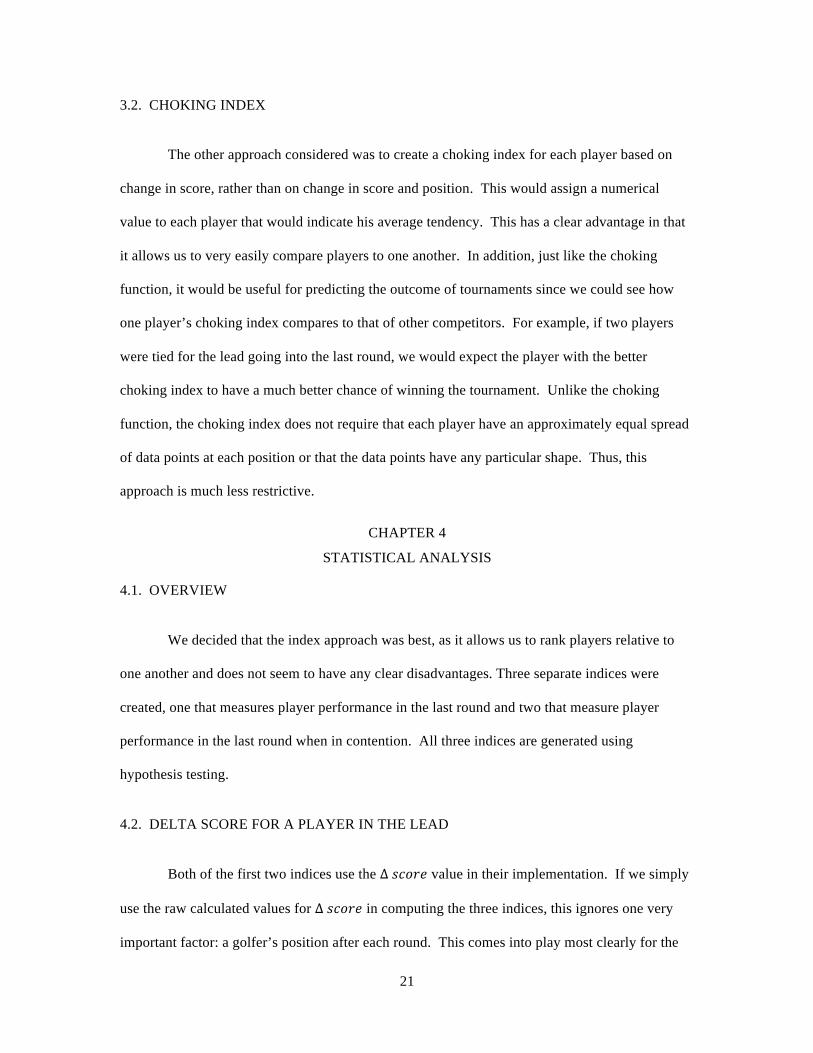
golfer with the lead going into the final round who goes on to win the tournament. In other
words, the position after both rounds three and four is first place. To investigate this, we looked
at all tournaments in 2011. For all golfers, the correlation between ∆ !"#$% and ∆ !"#$%$"& is
very high at ! = .8988.
If we consider separately those golfers who are in the lead going into the last round and
hold on to win (represented by red dots in the scatterplot), then obviously all the Δ !"#$%$"&
values will be zero and the data will be perfectly correlated, with a horizontal line of best fit.
However, this group of data skews the group of all golfers as a whole since the correlation for
that data set is positive. Thus, if we remove these golfers from the data set, we should see an
even higher correlation.
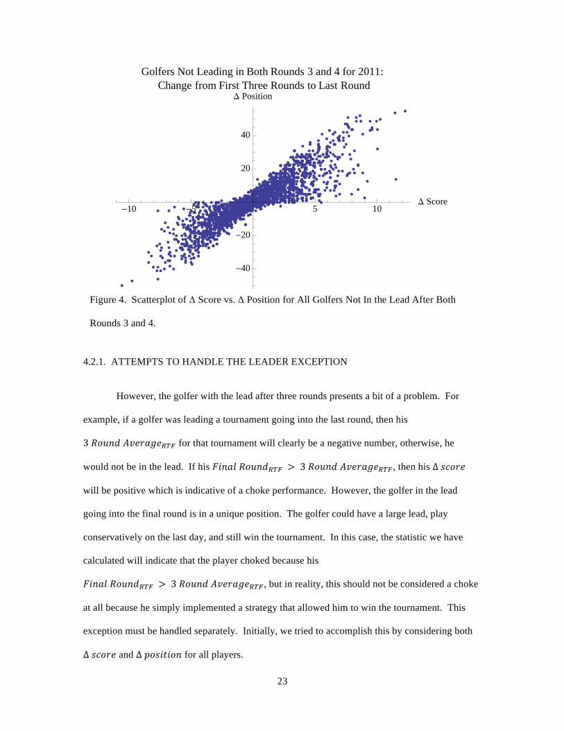
As expected, for all other positions, the correlation between ∆ !"#$% and ∆ !"#$%$"& is
even higher at ! = .9008, which allows us simply to use the Δ !"#$% value in analyzing player
performance, with the exception of the player leading going into the last round.
���� ��
��
�
����
�
�
�
�
��
���
�
��
�
�� �
�
�� � �
�
�� ����
��
�
�
�
�
�
�
�
�
�
�
�
�
�
�
�
�
��
�
��
���
�
��
���
�
�
�
�
�
�
�
�
�
�
��
��
�
�
�
�
��
�
�
�
��
�
�
� �
�
�
���
�
�
�
�
�
�
�
�
�
�
�
�
�
�
�
�
�
�
�
�
��
�
�
��
�
�
�
�
�
��
�
�
�
�
�
�
�
�
�
��
�
�
�
�
�
��
���
�
�
�
���
�
�
�
��
�
��
��
�
�
�
�
�
�
�
�
�
�
���
�
�
�
�
��
�
�
�
�
��
��
�
�
�
�
�
��
��
�
�
�
�
�
�
��
�
�
�
��
�
�
�
�
�
�
�
�
�
�
�
�
�
�
�
�
��
�
�
��
�
�
�
�
��
�
�
�
��
�
�
�
�
�
�
�
��
�
�
�
��
�
�
�
�
�
�
�
�
�
��
�
�
�
��
�
��
��
�
�����
�
�
�
�
���
�
�
�
�
��
��
������
���
�
�
�
�
�
�
�
�
�
����
�
�
�
����
�
�
�
�
�
�
�
�
�
�
�
�
�
�
�
�
�
���
��
�
�
�
�
�
�
��
�
��
��
��
�
��
�
�
�
��
�
�
�
� ����
�
��
� � ��
���
�
�
�
��
�
�
��
�
�
�
�
�
�
��
�
�
�
�
�
�
��
�
�
�
�
�
�
�
�
�
��
�
�
�
�
�
�
��
��
�
�
�
�
�
�
�
�
�
�
�
�
���
� ���
���
�
� ��
�
�
�
��
�
��
�
�
�
�
�
�
�
���
�
�
�
�
�
�
�
�
�
�
�
��
�
�
�
�
�
�
��
�
�
�
�
�
��
�
��
�
�
��
�
�
���
�� �� �
��
�
�
���
��
�
�
��
�
�
�
�
�
�
�
�
��
���
�
�
�
�
���
�
��
�
�
�
�
�
�
�
��
�
�
�
��
�
�
��
�
�
�
��
��
�
���
� ��
�
��
�
�
���
��
�
��
�
�
�
�
�
�
�
�
�
�
�
�
�
�
�
�
�
�
�
��
�
�
��
�
�
�
�
�
�
�
��
�
��
�
�
�
�
�
�
�
��
�
�
�
�
��
�
�
��
�
��
�
�
�
�
�
�
�
�
�
�
��
�
�
�
�
�
�
�
�
�
�
�
�
��
�
�
�
��
�
�
�
�
�
�
�
�
�
�
�
�
�
�
�
��
��
�
�
�
��
�
�
��
��
�
�
�
��
�
�� � ��
�
�
����
�
�
�
�
�
�
���
��
��
��
��
��
�
��
�
�
�
�
�
�
�
�
�
���
�
�
��
�
�
�
�
���
�
�
��
�
�
�
�
� �
�
��
�
�
�
�
�
�
�
�
� �
� ��
��
�
��
�
�
�
�
���
���
��
����
�
�
�
�
��
�
�
��
��
��
�
��
�
����
��
��
��
�
�
�
��
�
�
�
�
��
��
��
��
�
�
�
�
�
�
�
��
�
�
�
�
�
�
�
��
�
�
�
�
�
��
�
�
�
�
�
�
�
�
�
�
��
�
�
�
�
�
�
�
�
���
�
��
�
���
�
�
�
�
�
�
�
�
��
��
�
�
�
��
�
�
�
�
�
��
�
�
�
�
�
�
��
�
�
�
�
�
�
�
�
�
�
�
�
�
��
�
��
�
�
�
�
�
�
�
�
�
�
�
�
��
�
�
�
�
��
�
��
��
�
��
���
�
��
�
�
�
�
�
�
�
�
�
�
�
�
�
�
�
��
�
�
�
�
�
��
�
��
�
�
�
�
�
���
�
�
�
��
�
�
�
�
�
�
�
�
��
�
�
�
��
�
�
� � ���
�
� � �
���
��
��
�
��
�
�
�
��
�
�
�
�
��
�
�
�
�
��
�
�
��
�
�
�
�
��
�
�
��
�
��
�
�
�
�
�
�
��
�
�
�
�
�
��
�
�
�
�
�
�
�
��
��
��
��
��
�
��
�
�
�
�
�
�
�
�
�
�
�
�
�
�
�
�
�
�
�
�
��
�
�
�
�
�
�
�
�
�
��
�
�
�
�
��
�
�
�
�
�
�
�
��
�
�
�
��
�
���
�
��
��
��
�
��
���
�
�
�
�
�
�
�
�
�
�
�
��
�
�
�
�
�
�
�
��
��
�
�
��
�
�
�
�
�
�
�
��
�
�
�
�
�
�
��
�
�
��
�
�
�
�
�
�
�
�
��
� �
�
�
�
��
�
�
��
�
��
�
�
�
�
�
�
�
�
�
��
�
�
�
��
��
�
�
�
�
�
�
��
�
�
�
�
�
�
��
�
�
�
�
�
�
�
�
�
�
�
�
�
���
�
�
�
�
�
��
�
�
��
�
�
��
�
��
�
�
�
�
�
�
�
�
� �
�
�
�
�
��
�
�
�
��
�
�
�
�
��
�
�
�
�
�
�
�
�
�
�
�
�
�
��
�
�
�
�
�
�
�
�
�
�
�
�
�
�
�
�
�
�
�
�
���
��
�
�
�
�
�
��
�
�
�
��
��
�
�
�
�
�
�
�
��
�
�
�
�
�
�
�
�
�
�
��
��
�
�
�
��
�
���
�
�
��
��
��
�
�
�
��
�
�
� �
�
�
�
��
���
������
��
�
�
��
��
�
�
��
�
�
�
�
�
�
�
�
�
��
�
�
�
��
�
�
�
�
�� �
�
�
�
��
�
�
�
�
�
�
�
�
�
�
�
�
�
�
�
�
�
�
�
�
�
�
��
� ���
��
��
�����
��
�
�
�
�
�
�
�
�
�
�
�
�
�
�
��
�
�
�
�
�
�
�
�
�
�
��
�
�
�
�
�
�
�
�
�
�
�
�
�
�
�
��
�
�
�
�
��
�
�
��
� �
��
���
�
� �
�
�
�
�
�
��
�
�
�
��
�
��
�
��
�
�
�
�
�
�
�
�
�
�
��
�
�
��
�
�
�
�
�
�
�
�
�
�
�
�
�
�
�
�
�
�
�
�
�
�
�
��
�
�
�
�
�
�
�
�
�
�
��
� �
��
�
�
�
�
�
��
�
�
�
�
�
�
�
�
�
�
�
�
�
�
�
�
��
�
��
�
�
�
�
�
�
���
��
�
�
�
�
�
�
�
�
�
�
�
��
�
�
�
�
�
��
�
�
�
��
��
�
��
��
��
�
�
���
�
�
��
�
�
��
�
�
�
�
����
�
��
�
�
�
�
�
�
�
�
�
�
��
�
�
�
�
�
�
�
��
�
���
�
�
�
�
�
�
�
��
�
��
�
�
�
�
�
�
�
��
�
� �� �
�
�
�
�
�
��
�
�
�
�
�
��
�
�
�
����
�
�
�
��
�
�
�
�
�
�
��
�
�
�
�
�
��
�
��
�
�
��
�
�
��
�
�
��
�
�
�
���
�
�
��
�
��
��
�
��
�
�
�
�
�
�
�
�
�
�
�
�
���
�
�
�
�
�
�
�
�
�
�
�
�
�
��
�
�
�
�
�
�
�
�
�
�
�
�
�
�
�
�
�
�
��
��
�
��
��
�
�
�
�
�
�
��
�
���
�
�
�
�
�
��
�
�
�
��
��
�
�
�
�
�
�
�
�
�
�
�
�
�
�
�
�
�
�
�
�
�
�
�
��
�
�
�
�
�
�
�
�
�
�
��
�
�
�
�
�
�
�
�
�
�
�
�
�
�
�
�
�
�
�
�
�
��
��
�
�
�
��
�
�
�
�
�
�
� �
�
�
��
��
�
�
�
�
�
�
�
�
�
�
�
�
�
�
��
�
�
�
�
�
�
�
�
�
�
�
����
�
�
��
�
��
�
�
�
��
�
�
��
�
�
�
�
�
�
�
����
��
�
�� �
�
���
��
�
�
�
�
�
�
�
���
�
��
�
�
�
�
�
�
�
�
�
�
��
�
�
�
�
�
��
�
�
�
�
�
�
�
�
� �
�
�
�
� �
�
�
�
�
�
��
��
�
�
� �� �
�
��
�
�
�
��
�
�
�
�
�
�
�
��
�
�
�
�
���
�
�
�
�
�
�
�
�
�
��
�
��
�
��
�
�
�
�
�
��
�
�
�
�
�
�
��
�
�
�
���
��
�
�
�
�
�
�
�
�
�
�� ��
��
�
�
�
�
�
�
�
�
�
�
�
�
�
�
�
�
��
�
�
�
�
�
�
�
�
�
�
�
�
�
�
�
�
�
�
�
�
�
�
�
�
�
�
�
�
�
�
�
�
�
�
�
�
�
�
�
���
�
�
�
�
�
�
��
�
��
� �
�
��
�
�
�
�
�
�
�
�
�
�
�
�
�
�
�
�
�
�
�
�
�
�
�
���
�
�
�
�
�
�
�
���
�
�
�
�
�
�
�
�
�
��
�
�
��
�
�
�
�
��
�
�
��
�
�
�
�
��
�
�
����
�
�
�
�
�
�
�
� ��
��
�
�
�
�
�
�
�
�
�
�
�
�
�
�
���
�
�
�
�
�
�
�
�
� �
�
�
�
�
�
�
�
�
�
�
�
�
�
�
�
�
��
�
�
��
���� � ���
�
��
�
�
��
�
��
�
��
�
��
��
�
�
��
���
� �� �
�
�
��
��
�
��
��
�
���
�
�
�
�
�
�
�
�
�
�
�
�
�
�
�
�
�
�
�
��
�
�
�
�
�
�
�
�
�
�
��
�
�
��
�
�
�
�
��
�
�
�
�
�
�
�
��
�
�
��
� ���
�
�
�� �
�
�
�
�
�
�
��
�
�
�
��
�
�
�
�
�
�
�
�
�
��
�
�
�
�
�
��
�
�
�
��
�
�
�
��
�
�
�
�
�
���
�
�
�
�
���
���
�
�
�
��
�
��
��
�
��
�
�
��
��
�
�
��
��
��
�
�
�
�
�
�
�
�
�
�
�
�
���
�
�
�
�
�
�
� ��
�
��
�
�
�
��
�
�
�
�
�
��
�
�
�
�
�
��
�� �
�
��
�
�
�
�
�
�
�
�
�
�
�
�
�
�
�
�
�
���
�
�
�
�
�
�
�
�
�
�
�
�
�
�
��
�
�
�
�
��
�
�
�
�
�
�
�
�
�
�
�
�
�
�
�
�
��
�
�
�
�
�
�
�
�
�
�� �� � �� ��� ��� ��� �� � ���10 �5 5 10
� Score
�40
�20
20
40
� Position
Each Golfer in Each Tournament for 2011:Change from First Three Rounds to Last Round
Figure 3. Scatterplot of Δ Score vs. Δ Position for All Golfers With Leaders Emphasized.
23
4.2.1. ATTEMPTS TO HANDLE THE LEADER EXCEPTION
However, the golfer with the lead after three rounds presents a bit of a problem. For
example, if a golfer was leading a tournament going into the last round, then his
3 !"#$% !"#$%&#!"# for that tournament will clearly be a negative number, otherwise, he
would not be in the lead. If his !"#$% !"#$%!"# > 3 !"#$% !"#$%&#!"#, then his ∆ !"#$%
will be positive which is indicative of a choke performance. However, the golfer in the lead
going into the final round is in a unique position. The golfer could have a large lead, play
conservatively on the last day, and still win the tournament. In this case, the statistic we have
calculated will indicate that the player choked because his
!"#!" !"#$%!"# > 3 !"#$% !"#$%&#!"#, but in reality, this should not be considered a choke
at all because he simply implemented a strategy that allowed him to win the tournament. This
exception must be handled separately. Initially, we tried to accomplish this by considering both
Δ !"#$% and Δ !"#$%$"& for all players.
�10 �5 5 10� Score
�40
�20
20
40
� Position
Golfers Not Leading in Both Rounds 3 and 4 for 2011:Change from First Three Rounds to Last Round
Figure 4. Scatterplot of Δ Score vs. Δ Position for All Golfers Not In the Lead After Both
Rounds 3 and 4.

24
The first approach to tackling this problem was to consider the choking index (CI) as a
linear combination of the ∆ !"#$% and the ∆ !"#$%!"#, where ∆ !"#$%$"& > 0 indicates the player
lost position, ∆ !"#$%$"& < 0 indicates the player gained position and ∆ !"#$%$"& = 0 indicates
the player maintained his position. So, we now have
!" = !(∆ !"#$%) + !(∆ !"#$%!"#).
However, this presents a problem when the player does not change position from the
third round to the fourth round because the ∆ !"#$%$"& term would zero out and the CI would
then be entirely based on the ∆ !"#$%. This is acceptable for golfers in all positions except for the
lead. Still, the golfer who leads going into the last day, plays conservatively, but retains the lead,
would be considered to have choked because his CI would again be based entirely upon his
∆ !"#$%. Thus, no matter what values we choose for ! and !, this approach does not handle the
exception well.
Therefore, we next considered some type of interaction term in front of the ∆ !"#$%
piece. We want some type of term that will zero out if the position after round 3, call it !!, and
position after round 4, call it !!, are both one, such as (!!!! − 1). This term would zero out the
∆ !"#$% piece when the golfer is in the lead and retains the lead, and would be positive otherwise,
increasing as the golfer got farther away from the lead. We could also consider this term divided
by !!!!, which is equivalent to (1 − !!!!!
). This term would also zero out the ∆ !"#$% when the
golfer is in the lead and retains the lead but would now approach 1 as the golfer got farther away
from the lead. This type of term would provide additional information because it is important to
consider not only the ∆ !"#$%$"& term but also the !! and !! terms themselves, because, for
example, even though in the following two scenarios ∆ !"#$%$"& = 5, a change in position from
27th to 32nd is not nearly as bad as a change from 1st to 5th. Thus, we want the ∆ !"#$% term to

25
contribute more when the player is far from the lead and less when close to the lead. Finally, we
could also consider the sign (positive or negative) of ∆ !"#$%$"& by using the sign function
defined as
!"# ! = −1, ! < 0+1, ! ≥ 0.
This would indicate whether the golfer gained (-) or lost (+) position. Combining both of these
together, we have an interaction term defined as
!"#$%&'#!(" !"#$ = !"#(∆!"#$%$"&)(1 − !!!!!
).
Then, the modified linear combination would be
!" = !(!"#$%&'#!(! !"#$)∆!"#$% + !∆!"#$%$"&.
To determine the ideal constants ! and !, we would perform multiple linear regression on the
data set [7].
4.2.2. SIMPLIFIED HANDLING OF THE LEADER EXCEPTION
However, the main goal of implementing the linear combination of Δ !"#$% and
Δ !"#$%$"& was to handle the exception where the golfer with the 54 hole lead held on to win the
tournament, but played conservatively on the last day. In this case, the change in position is zero,
so the ∆ !"#!"!#$ term would always drop out. We attempted to find some type of interaction
term in front of the ∆ !"#$% term so that it would also drop out when the positions after rounds
three and four were both one. Thus, a much simpler solution is to set up an if-statement that
26
checks if !! and !! are both one and if ∆ !"#$% > 0. If both these conditions hold, then we
replace the calculated ∆ !"#$% with 0, to indicate that the player did not have a choke nor a clutch
performance. Although the player was unable to keep up the scoring pace that he had the first
three days, indicating that he performed worse than expected on the last day, he may have
intentionally played conservatively on the last day due to the lead that he had built up over the
first three days. Since he retained the lead and won the tournament, that performance cannot be
classified as a choke. This rewards a player who maintained his lead by playing better than
expected on the last day (a negative ∆ !"#$%), but does not punish a positive ∆ !"#$%. For all
other players, including players who had the lead going into the last round and did not end up
winning the tournament, the calculated ∆ !"#$% value is used. For the remainder of the paper,
∆ !"#$% will refer to the ∆ !"#$% value obtained using this procedure.
4.3. PERFORMANCE IN THE LAST ROUND
As explained in Section 2.2, we can find the mean ∆ !"#$% for each player denoted by
!∆ !"#$%. We can then perform a hypothesis test for each player to determine if the player chokes
or is clutch in the last round. We chose to perform a one-tailed test, rather than a two-tailed test,
because the one-tailed test indicates not only if a player’s mean value differs significantly from
zero, but in which direction it differs. Due to the fact that the variances of our populations are
unknown and that many players have sample sizes less than thirty (because they played in less
than thirty tournaments in the two year period), we used a one-sample t test for each player to test
the hypotheses. Each test was performed with the assumption that !∆ !"#$% = 0 for every player.
The alternative hypothesis depended on the value of !∆ !"#$%. If !∆ !"#$% > 0, then the test had
the following null and alternative hypotheses:
!!: !∆ !"#$% = 0

27
!!: !∆ !"#$% > 0.
If the test yielded a low p-value, then we could reject the null hypothesis and conclude that a
player’s !∆ !"!"# is likely greater than zero, indicating that the player tends to choke in the last
round.
Conversely, if !∆ !"#$% < 0, then the alternative hypothesis used was:
!!: !∆ !"#$% < 0.
With this test, a low p-value allowed us to reject the null hypothesis again, but now led to the
conclusion that the player’s !∆ !"#$% is likely less than zero, indicating that the player tends to be
clutch in the last round. With both tests, if the p-value is not sufficiently low, then we fail to
reject the null hypothesis, thus we cannot make any conclusive judgments about the player’s
tendency in the last round.
4.3.1. CHOICE FOR LEVEL OF SIGNIFICANCE
We must choose a value for !, the level of significance, with which to base our
conclusions regarding the p-values. Common values are ! = 0. 01, 0.05, or 0.10. We chose
! = 0.10 as the significance level.
Since the consequences of a Type 1 error (classifying a player as a choker when they are
not really a choker or classifying a player as clutch when they are not really clutch) are not
terribly serious, a larger value for ! is appropriate in this situation [8].
The smaller the value we choose for !, the fewer the number of players we can classify
as statistically significant chokers or clutch players, and the larger the value we choose, the
greater the number of players we can group into these two categories. However, since we are

28
attempting to rank players relative to one another, the value we choose for ! does not really
matter much in the long run, as it does not affect the rankings. However, the calculation of p-
values gives us additional information that a simple ordinal ranking of players does not provide.
4.3.2. SCALE THAT RANKS PLAYERS RELATIVE TO EACH OTHER
The p-value for this test tells us whether the player is a significant choker or significantly
clutch in the last round. However, regardless of whether the p-value is less than our specified
value for !, we can use the p-values for each player to rank them relative to each other. Recall
that for a hypothesis test, the p-value generated will always be between 0 and 1, because it is a
probability. Specifically, the p-value gives the probability that our sample would have the given
mean if the null hypothesis is true.
However, since we conducted the same type of test for each player with a different
alternative hypothesis depending on the sign of !∆ !"#$%, our p-value for each player can imply
two different things and our range for p-values is restricted. Since the sign of !∆ !"#$% dictated
which tail on which we chose to base the one tailed test, the probability cannot be greater than .5.
Thus our range for p-values is between 0 and .5. A small p-value can indicate either a tendency
to choke or be clutch depending on the alternative hypothesis of the test. Thus, if we use the p-
values for each player to create a ranking system, we must distinguish between these two
possibilities. We want to create a ranking scale that is easily understandable by the general
public, so we chose to let the scale range from positive to negative, which indicates chokers and
clutch players respectively. A simple solution would be to multiply the p-value by 1 if
!∆ !"#$% > 0 and multiply by -1 if !∆ !"#$% < 0. This would give us a scale that ranges from -.5 to
0 and 0 to .5. However, with this scale, a value of -.5 indicates a player who is certainly clutch
and a value of .5 indicates one who is certainly a choker. Since 1 and -1 are typically the values
associated with “perfect” probabilities in statistics, we chose to fit our ranking scale to this
convention. This can be accomplished in a fairly simple way. Rather than using 1 or -1 as a

29
scaling factor, we use −2×!"#$%& + 1 and 2×!"#$%& − 1 respectively. This gives us a
scale that ranges from -1 to 1, with -1 indicating a player who is certainly clutch, 1 indicating a
player who is certainly a choker, and 0 indicating a player who does not have a tendency to choke
nor be clutch but instead performs exactly as the typical golfer does.
4.3.3. EXPLANATION OF THE PROCESS WITH AN EXAMPLE
For clarity, we illustrate the process with one player. Consider Rory McIlroy, two-time
major champion. Out of the twenty tournaments (! = 20) in which McIlroy participated in 2011
and 2012, his !∆ !"#$% = 1.1016 with a sample standard deviation of ! = 3.2032. Since his
!∆ !"#$% is positive, our alternative hypothesis is !!: !∆ !"#$% > 0. Thus, McIlroy’s t statistic is
! = !!!!/ !
= !.!"!#!!!.!"#!/ !"
= 1.5380. The p-value is obtained by the density function of the t
distribution with ! = ! − 1 = 20 − 1 = 19 degrees of freedom. McIlroy’s p-value is ! =
0.0703, thus we can reject the null hypothesis and conclude that he is a statistically significant
choker. To determine his placement on the choking index scale, we observe that !∆ !"#$% > 0
which means that McIlroy’s index is −2×!"#$%& + 1 = −2×0.0703 + 1 = 0.8595. This
places McIlroy relatively close to the bottom of the rankings for all players, an interesting finding
given that McIlroy is a highly ranked player.
4.3.4. BEST AND WORST RANKED PLAYERS
This process was repeated for all players. The following table gives the best (most
clutch) and worst (most choking) ranked players. Indices for all remaining players can be found
in the Appendix.
PLAYER NAME CIΔ score RANK Donald, Luke -0.9996 1 Choi, K.J. -0.9936 2 Rose, Justin -0.9927 3 Schwartzel, Charl -0.9861 4

30
Allenby, Robert -0.9848 5 Slocum, Heath -0.9843 6 Poulter, Ian -0.9839 7 Ogilvy, Geoff -0.9837 8 Westwood, Lee -0.9823 9 Funk, Fred -0.9794 10 --------------------------- ---------------- -------------- Marino, Steve 0.9176 343 Leonard, Justin 0.9338 344 Atwal, Arjun 0.9394 345 Connell, Michael 0.9397 346 Green, Nathan 0.9419 347 Gainey, Tommy 0.9445 348 Tidland, Chris 0.9553 349 Palmer, Ryan 0.9823 350 Biershenk, Tommy 0.9853 351 Gangluff, Stephen 0.9878 352
4.4. PERFORMANCE IN THE LAST ROUND WHEN IN CONTENTION
As described in Section 2.3, analyzing player performance when in contention involves
dividing the ∆ !"#$% values into two groups and then calculating !!" and !!" . In this case, we
needed to perform a two-sample t test for each player.
Each test was performed with the assumption that the two ∆ !"#$% means are equal for
each player. The alternative hypothesis depended on the value of !!" − !!" . If !!" − !!" > 0,
then the test had the following null and alternative hypotheses:
!!: !!" − !!" = 0
!!: !!" − !!" > 0.
If the test yields a low p-value, then we could reject the null hypothesis and conclude that a
player’s !!" is likely higher than his !!" , indicating that the player tends to choke when in
contention.
Table 1. Best Ten and Worst Ten Choking Indices: Performance in the Last Round

31
Conversely, if !!" − !!" < 0, then the alternative hypothesis we used was:
!!: !!" − !!" < 0.
With this test, a low p-value allowed us to reject the null hypothesis again, but now leads to the
conclusion that the player’s !!" is likely less than his !!" , indicating that the player tends to be
clutch when in contention. With both tests, if the p-value is not low, then we failed to reject the
alternative hypothesis, thus we cannot make any conclusive judgments about the player’s
tendency when in contention.
4.4.1. STUDENT’S T TEST FOR INITIAL TESTING
Initially, we conducted this test (with the appropriate null and alternative hypotheses) for
each player as a standard two-sample t test for differences in means. The t test was chosen
because the sample sizes used to compute !!" and !!" for nearly all players were not large
enough to invoke the Central Limit Theorem. In addition, the parameters !!" and !!" are not
known [7]. The only requirements for this test are that samples are independent random samples
from two normal populations having the same unknown variance !!.
At first, we considered the entire field’s data from the two years to be the population and
treated each player’s data over the two-year period as a random sample from the population.
Then the sample statistics computed for the field can be considered the parameters for the
population. Technically, this is not exactly a random sample since the sample consists of data
entirely from one player, but if each player is chosen randomly this is not too much of a concern.
In treating each player’s data set as a sample from the population with known parameters, we
essentially were conducting a hypothesis test in reverse: the parameters were known and we
wanted to determine the probability of the sample statistic’s occurrence given the parameter.
This would tell us if a player deviated from the field’s typical behavior.
32
In initial tests, performed with data from 2011 only and with in contention defined as
within eight shots of the lead, the variances of the two populations, the field in contention and the
field out of contention, were very close to equal, with values of 8.3953 and 8.4980 respectively.
Thus, the conditions for a standard two-sample t test are sufficiently met in this case. However,
when the value defining in contention was changed to four, and data from both 2011 and 2012
was included, this condition no longer held. The population variances were no longer close to
equal. Clearly, the standard two-sample t test is no longer an appropriate test to conduct.
4.4.2. RECASTING THE POPULATION DEFINITION
Since some of the assumptions for the situation specified above were somewhat forced,
we decided to alter the approach. Rather than consider the field to be the population, we chose to
use a more conventional definition for the population: all scores for all PGA Tour players for all
time. Then all scores for the field for the two years is a sample of this population. When
considering players individually, the population is defined as all scores for that player for all time
and the scores for the two-year time period are a sample of this population. Then, when the t tests
are conducted, we have no way of knowing whether the population’s variances are equal (either
!!!"! vs. !!!"! for analysis of the field’s tendencies or !!!"! vs. !!!"! for analysis of
individual player tendencies). Clearly, the standard two-sample t test is no longer appropriate.
4.4.3. FINDING AN SUITABLE TEST
The populations are still assumed to be normal. When examining histograms of the data
from the two years, which are very large samples from the populations, they appear to be
somewhat bell-shaped and not strongly skewed. Thus, assuming a normal distribution seems
reasonable.

33
However, we no longer have the luxury of assuming that the two normal populations
have equal variances. Thus, we must find another type of test that meets the new conditions.
Upon investigating the various types of tests available, we chose to use the t test for
unequal variances. There are three main types of tests to test differences in the means of two
different groups, the standard student’s t test, the Mann-Whitney U test, and the t test for unequal
variances. The latter two tests are underutilized in research, even though they provide a great
deal more flexibility than student’s t test [9].
The Mann-Whitney U test is an efficient test when the two populations are not normally
distributed, however, since our populations are assumed to be approximately normal, this test
provides no sizable advantage. With student’s t test, unequal variances cause less error when
sample sizes are similar, but as the sample sizes become more unequal, the test becomes
increasingly more unreliable. Since nearly all players are out of contention much more often than
they are in contention, the sample sizes are far from equal. So, we are left with the third option,
the test for unequal variances. Of interest is the fact that the unequal variance t test performs just
as well as student’s t test when the population variances are equal, so using this test does not have
any clear disadvantages [9]. Importantly, this test allows us to compare means when the
variances of the population are unknown and unequal, as well as when sample sizes are unequal,
which are the precise conditions that we have.
�5 0 5 10� Score
50
100
150
200
CountIn Contention � Scores For All Players
�10 �5 0 5 10� Score
200
400
600
800
CountOut of Contention � Scores For All Players
Figure 5. Histograms of In Contention and Out of Contention Δ Scores For All

34
Thus, we will use the t test for unequal variances, also known as Welch’s t test or the
Smith-Satterthwaite test, to test our data.
4.4.4. DESCRIPTION OF WELCH’S T TEST
With this test, the null hypothesis is !!: !! − !! − ! = 0. The test statistic is computed
by
! =!! − !! − !
!!!!!+ !!!!!
and the number of degrees of freedom is computed by
! =(!!!
!!+ !!!!!)!
(!!! !!)!
!! − 1+ (!!
! !!)!
!! − 1
where ! is rounded down to the nearest integer. The following are the definitions of the
variables:
!!: Mean of the first sample
!!!: Variance of the first sample
!!: Number of data points in first sample
!!: Mean of the second sample
!!!: Variance of the second sample
!!: Number of data points in second sample
!: Assumed difference in the means of the two groups [10].
4.4.5. RESULTS OF WELCH’S T TEST
Since sample variance is undefined when the sample size is less than two and this test
requires the sample variances for both samples in its calculations, players who were in contention

35
(or out of contention) less than two times were removed from the data set. This does not lead to a
significant loss in utility since we can not draw very reliable conclusions anyway about the
tendency of a player who is only is contention or out of contention once or not at all.
When Welch’s t test was performed for each player (again, using the corresponding
alternative hypothesis, depending on the sign of !!" − !!"), there were many players whose p-
value allowed us to reject the null hypothesis when !!: !!" − !!" > 0, but very few that allowed
us to reject the null when !!: !!" − !!" < 0. This led to the suspicion that the field (in other
words, the typical player) chokes when in contention, on average.
To investigate this suspicion, we performed the same Welch’s t test again, but this time,
using the data set for the entire field, rather than grouping the data into subsets by player as
before. Since !!" − !!" > 0 for the field, our alternative hypothesis was
!!: !!" − !!" > 0.
The p-value for this test was ! = 1.6902 × 10!!", thus, we can reject the null hypothesis
!!: !!" − !!" = 0
with near certainty. With two years of data, !! = 672 and !! = 5211, so we can be assured that
the test is very reliable when applied to the field. Although we do not know the actual values of
the field’s parameters !!" and !!" , with such large sample sizes, we can use the sample statistics
!!" = 1.6128 and !!" = −0.2154, respectively, as reasonable approximates for the parameters.
Thus, !!" − !!" = 1.8282, hence the typical golfer shoots about two strokes worse when in
contention on the last day.
With this in mind, the application of Welch’s t test to all players individually, with

36
!!: !!" − !!" = 0
is inherently unfair. It ignored the reality for the field that
!!" − !!" > 0.
Essentially, our null hypothesis assumed that distribution was a standard t distribution centered at
zero, when in fact it was a noncentral t distribution [11]. As Figure 4 demonstrates, this can lead
to major errors in the p-values obtained. Therefore, in order to create a fair test, each player
needs to be tested relative to the field. This will bring the distribution back to the standard t
distribution centered at zero.
Figure 6. Noncentral T Distributions
�5 5 10
0.05
0.10
0.15
0.20
0.25
0.30
0.35
Centered at 0
Centered at 1.8282
Noncentral T Distributions: Different Centers, Same Degrees of Freedom
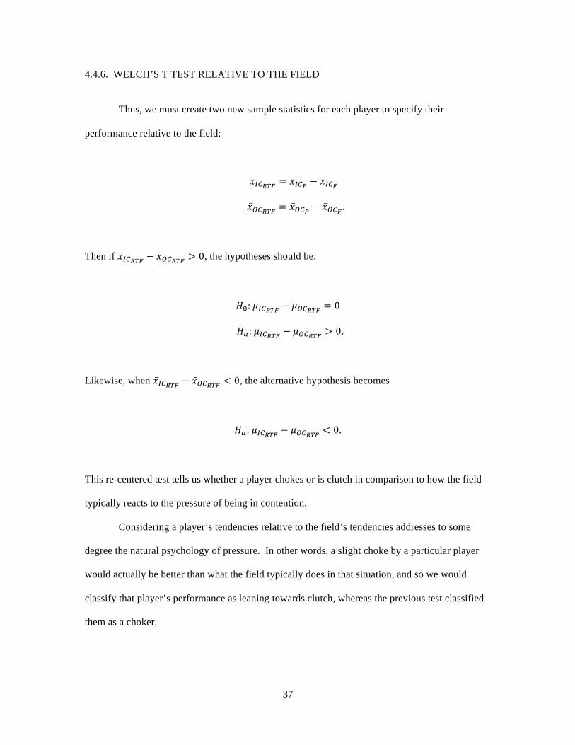
37
4.4.6. WELCH’S T TEST RELATIVE TO THE FIELD
Thus, we must create two new sample statistics for each player to specify their
performance relative to the field:
!!"!"# = !!"! − !!"!
!!"!"# = !!"! − !!"!.
Then if !!"!"# − !!"!"# > 0, the hypotheses should be:
!!: !!"!"# − !!"!"# = 0
!!: !!"!"# − !!"!"# > 0.
Likewise, when !!"!"# − !!"!"# < 0, the alternative hypothesis becomes
!!: !!"!"# − !!"!"# < 0.
This re-centered test tells us whether a player chokes or is clutch in comparison to how the field
typically reacts to the pressure of being in contention.
Considering a player’s tendencies relative to the field’s tendencies addresses to some
degree the natural psychology of pressure. In other words, a slight choke by a particular player
would actually be better than what the field typically does in that situation, and so we would
classify that player’s performance as leaning towards clutch, whereas the previous test classified
them as a choker.
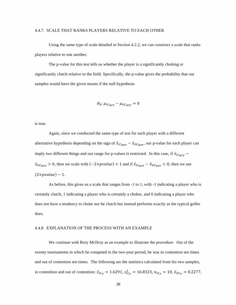
38
4.4.7. SCALE THAT RANKS PLAYERS RELATIVE TO EACH OTHER
Using the same type of scale detailed in Section 4.2.2, we can construct a scale that ranks
players relative to one another.
The p-value for this test tells us whether the player is a significantly choking or
significantly clutch relative to the field. Specifically, the p-value gives the probability that our
samples would have the given means if the null hypothesis
!!: !!"!"# − !!"!"# = 0
is true.
Again, since we conducted the same type of test for each player with a different
alternative hypothesis depending on the sign of !!"!"# − !!"!"#, our p-value for each player can
imply two different things and our range for p-values is restricted. In this case, if !!"!"# −
!!"!"# > 0, then we scale with −2×!"#$%& + 1 and if !!"!"# − !!"!"# < 0, then we use
2×!"#$%& − 1.
As before, this gives us a scale that ranges from -1 to 1, with -1 indicating a player who is
certainly clutch, 1 indicating a player who is certainly a choker, and 0 indicating a player who
does not have a tendency to choke nor be clutch but instead performs exactly as the typical golfer
does.
4.4.8. EXPLANATION OF THE PROCESS WITH AN EXAMPLE
We continue with Rory McIlroy as an example to illustrate the procedure. Out of the
twenty tournaments in which he competed in the two-year period, he was in contention ten times
and out of contention ten times. The following are the statistics calculated from his two samples,
in contention and out of contention: !!"! = 1.6291, !!"!! = 16.8323, !!"! = 10, !!"! = 0.2277,
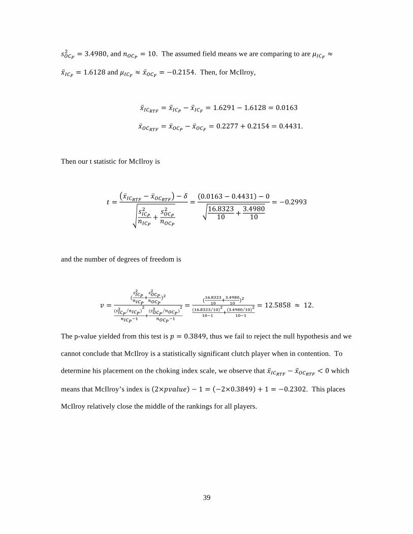
39
!!"!! = 3.4980, and !!"! = 10. The assumed field means we are comparing to are !!"! ≈
!!"! = 1.6128 and !!"! ≈ !!!! = −0.2154. Then, for McIlroy,
!!"!"# = !!"! − !!"! = 1.6291 − 1.6128 = 0.0163
!!"!"# = !!"! − !!"! = 0.2277 + 0.2154 = 0.4431.
Then our t statistic for McIlroy is
! =!!"!"# − !!"!"# − !
!!"!!
!!"!+!!"!!
!!"!
=0.0163 − 0.4431 − 0
16.832310 + 3.498010
= −0.2993
and the number of degrees of freedom is
! =(!!"!!
!!"!!!!"!!
!!"!)!
(!!"!! !!"!)
!
!!"!!!!(!!"!! !!"!)
!
!!"!!!
=(!".!"#"!" !!.!"#$!" )!
(!".!"#" !")!
!"!! !(!.!"#$ !")!
!"!!
= 12.5858 ≈ 12.
The p-value yielded from this test is ! = 0.3849, thus we fail to reject the null hypothesis and we
cannot conclude that McIlroy is a statistically significant clutch player when in contention. To
determine his placement on the choking index scale, we observe that !!"!"# − !!"!"# < 0 which
means that McIlroy’s index is 2×!"#$%& − 1 = −2×0.3849 + 1 = −0.2302. This places
McIlroy relatively close the middle of the rankings for all players.

40
4.4.9. BEST AND WORST RANKED PLAYERS
This process was repeated for all players. The following table gives the ten best and ten
worst ranked players according to this scale. Indices for all remaining players can be found in the
Appendix.
PLAYER NAME CIIC Δ score RANK Henry, J.J. -0.9967 1 Walker, Jimmy -0.9908 2 Rocha, Alexandre -0.9906 3 Beckman, Cameron -0.9885 4 Palmer, Ryan -0.9846 5 Clark, Tim -0.9613 6 Kuchar, Matt -0.9568 7 Simpson, Webb -0.9510 8 Vegas, Jhonattan -0.9436 9 Goydos, Paul -0.9278 10 --------------------------- ---------------- -------------- Estes, Bob 0.9097 139 Merrick, John 0.9339 140 Rose, Justin 0.9629 141 Claxton, Will 0.9684 142 McDowell, Graeme 0.9778 143 Appleby, Stuart 0.9848 144 Davis, Brian 0.9984 145 Villegas, Camilo 0.9992 146 Gomez, Fabian 0.9998 147 Cink, Stewart 1.0000 148
4.4.10. WELCH’S T TEST USING FOURTH ROUND RELATIVE TO THE FIELD
While the ∆ !"#$% value indicates whether a player kept up his scoring pace that was
established in the first three rounds, if we consider only how a player performed in the last round
relative to the field, we can determine which players truly had extreme performances. For
example, a player who did not play as well in the last round as his first three rounds would have
been classified as a choker in the previous scale. If he also played worse than the field average in
Table 2. Best Ten and Worst Ten Choking Indices: Performance in the Last Round In Contention, Δ Score

41
the last round when in contention, then clearly the player fell off his scoring pace by a sizable
amount. The opposite holds true for those players with great performances. Thus, this creates a
secondary index that can be used to measure the severity of changes regarding performance in
contention. The same type of hypothesis test was conducted for each player but with
!"#$% !"#$%!"# used in place of ∆ !"#$%. As this process in nearly identical to the one detailed
in Section 4.4.8, the calculation for our example player, Rory McIlroy, will not be demonstrated.
Again, the rankings were tabulated in the same manner as above. The following are the
players with the best ten and the worst ten rankings. Indices for all remaining players can be
found in the Appendix.
PLAYER NAME CIIC 4th round RANK Frazar, Harrison -0.9987 1 Walker, Jimmy -0.9867 2 Baird, Briny -0.9861 3 Beckman, Cameron -0.9664 4 Goydos, Paul -0.9605 5 Palmer, Ryan -0.9505 6 Vegas, Jhonattan -0.9248 7 Campbell, Chad -0.8950 8 Mickelson, Phil -0.8820 9 Wilson, Mark -0.8749 10 --------------------------- ---------------- ---------------- Merrick, John 0.9305 139 Stricker, Steve 0.9345 140 McDowell, Graeme 0.9562 141 Rose, Justin 0.9786 142 Davis, Brian 0.9801 143 Claxton, Will 0.9915 144 Appleby, Stuart 0.9959 145 Gomez, Fabian 0.9998 146 Villegas, Camilo 0.9999 147 Cink, Stewart 1.0000 148
.
Table 3. Best Ten and Worst Ten Choking Indices: Performance in the Last Round In Contention, Fourth Round
42
4.5. CONCLUSION
Thus far, we have examined the performance under pressure of all PGA Tour golfers in
the years 2011 and 2012. Two main pressure scenarios were considered: the pressure of the last
round of a tournament, and the additional pressure of the last round of a tournament when in
contention. Three indices were constructed to rank players relative to one another. The first
index, which describes the reaction to the pressure of the last round, was constructed using the
probabilities generated by a one-sample t test regarding the mean ∆ !"#$% value for a player in all
tournaments. The second two indices, which both describe the reaction to the pressure of the last
round when in contention, were constructed using the probabilities generated by Welch’s t tests
regarding the difference in mean ∆ !"#$% values and !"#$% !"#$%!"# values, respectively, for a
player when in contention and when not in contention.
CHAPTER 5
PROPOSED FUTURE RESEARCH IDEAS
5.1. CHOKING INDEX FOR PLAYERS NEAR THE CUT LINE
We have created workable models for measuring performance under pressure on the last
day of tournaments and performance under pressure when in contention on the last day of a
tournament. The last pressure situation not yet considered is performance when the player is near
the cut line after the first day of play. Our model for measuring performance when in contention
could be readily adapted to measure performance in this situation. Rather than determining a
cutoff point for in contention, we would need to determine a cutoff point at which it is reasonable
to assume that the player has a decent chance at making or missing the cut. The main difference
is that this cutoff value could go in either direction, whereas the in contention value was one
sided. Many players will be ahead of the cut-line, but still close enough to it that they need to
worry about making the cut. The ∆ !"#$% value in this case would be the change in score relative
to the field from round one to round two. Then a hypothesis test with the appropriate hypotheses

43
could be conducted for each player to determine if his ∆ !"#$% is significantly different when
near the cut-line than it is when not near the cut line. Again, the final choking index would be a
scale between -1 and 1 that ranks players relative to one another. We expect that some players
may be clutch in one type of pressure situation and chokers in another.
5.2. TESTING THE NORMALLY DISTRIBUTED POPULATIONS ASSUMPTION
Although we assumed that the populations are normally distributed, we suspect that this
may not be the case. Thus, we need to test the populations for normality, and if our suspicions
are confirmed, we may need to alter the type of tests conducted. The Mann-Whitney U-test, a
nonparametric alternative to the t test, would be a leading candidate. In addition, it would be
possible to conduct our tests empirically by building our own distribution function based on the
data we have, rather than relying on a well-known distribution.
5.3. SPECIFIC PART OF THE GAME
If we conclude that a player has choked or been clutch in the past, given the multitude of
statistics that the PGA Tour keeps, we can find exactly which parts of the golfer’s game fell apart
or excelled. For example, we may find that some players choke because they hit wild drives and
others choke due to missing more putts than usual. This would be extremely valuable
information to the players, as it would allow them to know exactly what part of their game they
need to work harder at.
In psychological theory, this phenomenon can be explained using the Yerkes-Dodson
Law, which states that the relationship between arousal (the level of physiological activation of
the brain and body) and performance is best represented by an inverted U-shaped curve.
Therefore, there is an optimal level of arousal that maximizes performance. For our purposes, the
level of arousal can be considered the amount of pressure that is on the golfer. However, this
curve can shift based on what task is being performed. A well-learned task requires a higher
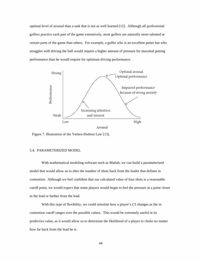
44
optimal level of arousal than a task that is not as well learned [12]. Although all professional
golfers practice each part of the game extensively, most golfers are naturally more talented at
certain parts of the game than others. For example, a golfer who is an excellent putter but who
struggles with driving the ball would require a higher amount of pressure for maximal putting
performance than he would require for optimum driving performance.
5.4. PARAMETERIZED MODEL
With mathematical modeling software such as Matlab, we can build a parameterized
model that would allow us to alter the number of shots back from the leader that defines in
contention. Although we feel confident that our calculated value of four shots is a reasonable
cutoff point, we would expect that some players would begin to feel the pressure at a point closer
to the lead or farther from the lead.
With this type of flexibility, we could simulate how a player’s CI changes as the in
contention cutoff ranges over the possible values. This would be extremely useful in its
predictive value, as it would allow us to determine the likelihood of a player to choke no matter
how far back from the lead he is.
Figure 7. Illustration of the Yerkes-Dodson Law [13].

45
5.5. INTIMIDATION INDEX
To determine how a particular player’s presence near the top of the leaderboard affects
the performance of other players, we can look at the ∆ !"#!" values for the other players in
contention. If a certain player intimidates the other golfers, then we would expect the ∆ !"#$%
values for the other players in contention to be positive on average, which might imply that the
player causes the other players to choke. If a certain player is not seen as a threat, then we would
expect the ∆ !"#$% values for the other players in contention to be negative on average, which
might imply that the player causes the other players to be clutch. If the ∆ !"#$% values for the
other players in contention are near zero on average, then the player in question has no effect one
way or another on the other players in contention. Using this type of logic, we can construct
another index called the intimidation index to rank the players relative to one another.

46
APPENDIX
PLAYER NAME CIΔ score CIIC Δ score CIIC 4th round
Henry, J.J. -0.7197 -0.9967 -0.7835 Walker, Jimmy -0.0292 -0.9908 -0.9867 Rocha, Alexandre 0.5961 -0.9906 -0.8391 Beckman, Cameron 0.8867 -0.9885 -0.9664 Palmer, Ryan 0.9823 -0.9846 -0.9505 Clark, Tim -0.3755 -0.9613 -0.8514 Kuchar, Matt 0.5072 -0.9568 -0.6511 Simpson, Webb 0.7805 -0.9510 -0.7876 Vegas, Jhonattan 0.0835 -0.9436 -0.9248 Goydos, Paul 0.8370 -0.9278 -0.9605 Mickelson, Phil 0.0276 -0.9186 -0.8820 Woods, Tiger -0.7798 -0.8898 -0.7333 Overton, Jeff -0.9385 -0.8804 -0.8021 O'Hair, Sean 0.4738 -0.8552 -0.7552 Frazar, Harrison 0.5352 -0.8472 -0.9987 Baird, Briny -0.0969 -0.8440 -0.9861 Hoffman, Charley -0.6931 -0.8418 -0.8093 Els, Ernie -0.0827 -0.8140 -0.8339 Wagner, Johnson 0.4304 -0.8002 -0.8081 Campbell, Chad -0.6676 -0.7961 -0.8950 Potter, Jr., Ted 0.9167 -0.7876 -0.7431 Kirk, Chris -0.8709 -0.7658 -0.8227 Lyle, Jarrod 0.1044 -0.7578 -0.7736 Leonard, Justin 0.9338 -0.7325 -0.7728 Wilson, Mark 0.1274 -0.7214 -0.8749 Moore, Ryan 0.4690 -0.6811 -0.6058 Couch, Chris 0.8798 -0.6487 -0.3272 Dufner, Jason 0.7609 -0.6387 -0.3995 Leishman, Marc 0.3280 -0.6372 -0.5425 Johnson, Zach -0.0529 -0.6369 -0.7661 Gainey, Tommy 0.9445 -0.6196 -0.4588 Snedeker, Brandt -0.7982 -0.6106 -0.4400 Gay, Brian -0.8192 -0.6088 -0.5957 Jones, Matt 0.8921 -0.5833 -0.7643 Hearn, David -0.4969 -0.5479 -0.6822 Beljan, Charlie -0.6232 -0.5063 -0.8038 Tringale, Cameron 0.8244 -0.4990 -0.5281 Points, D.A. -0.3804 -0.4916 -0.3832 Allenby, Robert -0.9848 -0.4752 -0.4178

47
Glover, Lucas 0.7817 -0.4556 -0.4476 Blixt, Jonas -0.0563 -0.4535 -0.6723 Every, Matt 0.4242 -0.4517 -0.3552 Bae, Sang-Moon 0.5499 -0.3691 -0.3052 Marino, Steve 0.9176 -0.3661 -0.3567 Noh, Seung-Yul -0.7357 -0.3545 -0.4129 Duke, Ken 0.3604 -0.3410 -0.3106 Ishikawa, Ryo -0.0357 -0.3174 -0.8148 Romero, Andres 0.0087 -0.3120 -0.3978 Beem, Rich 0.7930 -0.2844 -0.0705 Stenson, Henrik 0.7299 -0.2673 0.0170 Stallings, Scott -0.3487 -0.2604 -0.3139 Chappell, Kevin -0.0828 -0.2400 -0.3930 Chopra, Daniel 0.7979 -0.2353 0.2928 McIlroy, Rory 0.8595 -0.2302 -0.1857 Love III, Davis 0.7179 -0.2281 0.2625 Adams, Blake -0.8710 -0.2202 0.1146 Harrington, Padraig -0.2876 -0.1938 0.2530 McGirt, William -0.5394 -0.1614 0.0441 Kang, Sung -0.0388 -0.1564 -0.0295 Haas, Bill 0.7844 -0.1511 0.1073 Bradley, Keegan 0.3671 -0.1271 -0.1690 Schwartzel, Charl -0.9861 -0.1066 0.0069 Pettersson, Carl -0.9747 -0.1039 -0.3643 Verplank, Scott 0.1701 -0.0787 -0.2824 Haas, Hunter -0.5835 -0.0482 -0.2355 Garrigus, Robert -0.1595 -0.0340 -0.3234 Singh, Vijay 0.3293 -0.0323 -0.0933 Johnson, Dustin -0.5814 -0.0101 0.0081 Molder, Bryce -0.4268 -0.0011 0.0758 FIELD 0.0000 0.0000 0.0000 Stroud, Chris -0.3596 0.0054 -0.1231 McNeill, George -0.6677 0.0068 -0.2521 Reavie, Chez -0.3318 0.0295 0.0138 Durant, Joe -0.9344 0.0297 0.0814 Austin, Woody -0.1055 0.0308 0.5390 Howell III, Charles -0.4573 0.0337 0.5665 Laird, Martin 0.5721 0.0514 0.6773 Stanley, Kyle -0.3339 0.0640 -0.1184 Watson, Bubba -0.4221 0.0814 0.0206 Pernice Jr., Tom -0.8553 0.0869 -0.0350 Rollins, John -0.4287 0.0902 0.2677 Driscoll, James 0.2060 0.1115 0.1894

48
Gates, Bobby 0.8286 0.1410 0.2428 Atwal, Arjun 0.9394 0.1670 -0.0421 DeLaet, Graham 0.5707 0.1692 0.0427 Holmes, J.B. -0.0949 0.2046 0.3713 Sabbatini, Rory 0.0147 0.2131 0.4104 Watney, Nick -0.0691 0.2434 0.2857 Oosthuizen, Louis 0.4578 0.2536 -0.3328 Matteson, Troy 0.0409 0.2571 -0.2811 Cauley, Bud -0.9730 0.2593 0.3684 Choi, K.J. -0.9936 0.2684 0.0785 Hadwin, Adam 0.2147 0.3030 0.0492 Immelman, Trevor -0.0145 0.3037 0.3905 Crane, Ben -0.8258 0.3546 0.5477 Riley, Chris -0.7661 0.3575 0.5113 Trahan, D.J. -0.1516 0.3627 0.5635 Blanks, Kris -0.7833 0.3787 0.3358 Senden, John 0.6746 0.3794 0.8493 Thatcher, Roland -0.3354 0.4144 0.4991 Stricker, Steve 0.8663 0.4477 0.9345 Donald, Luke -0.9996 0.4487 0.8031 Teater, Josh -0.0990 0.4501 0.4628 Toms, David -0.9220 0.4593 0.5499 Woodland, Gary -0.1146 0.4676 0.5161 Maggert, Jeff 0.8907 0.4979 0.6915 Goosen, Retief -0.2687 0.5051 0.5110 Westwood, Lee -0.9823 0.5181 0.3362 Jacobson, Fredrik 0.7024 0.5215 0.6784 Levin, Spencer 0.0116 0.5325 0.5557 English, Harris 0.6372 0.5521 0.5169 O'Hern, Nick -0.3967 0.5590 0.5612 Summerhays, Daniel 0.8068 0.5888 0.6688 Fowler, Rickie 0.5503 0.5996 0.5645 Baddeley, Aaron -0.3415 0.6008 0.5947 Day, Jason -0.8769 0.6230 0.6162 Perez, Pat -0.3739 0.6290 0.7410 Byrd, Jonathan 0.7982 0.6609 0.4864 Garcia, Sergio -0.3810 0.6614 0.7167 Van Pelt, Bo -0.4402 0.6618 0.8884 Na, Kevin -0.8309 0.6750 0.6013 Scott, Adam -0.0751 0.6764 0.6472 Petrovic, Tim -0.5689 0.6862 0.7004 Karlsson, Robert -0.7368 0.7090 0.5399 Wi, Charlie 0.7438 0.7103 0.6529
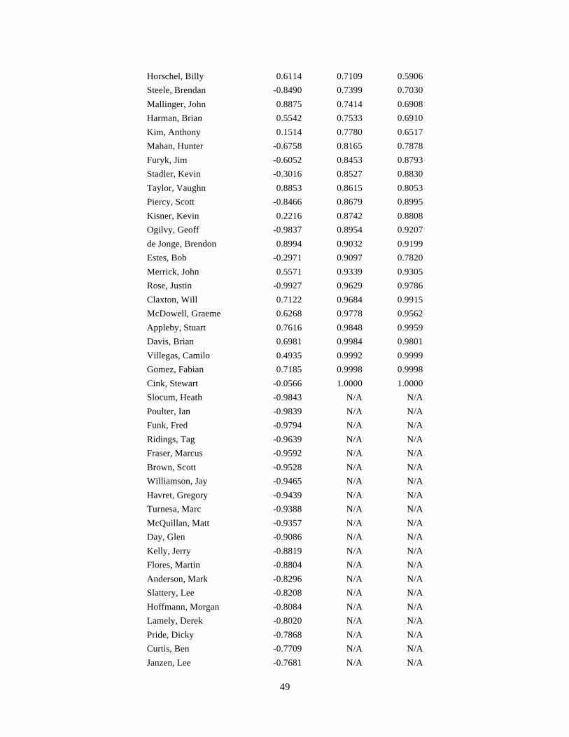
49
Horschel, Billy 0.6114 0.7109 0.5906 Steele, Brendan -0.8490 0.7399 0.7030 Mallinger, John 0.8875 0.7414 0.6908 Harman, Brian 0.5542 0.7533 0.6910 Kim, Anthony 0.1514 0.7780 0.6517 Mahan, Hunter -0.6758 0.8165 0.7878 Furyk, Jim -0.6052 0.8453 0.8793 Stadler, Kevin -0.3016 0.8527 0.8830 Taylor, Vaughn 0.8853 0.8615 0.8053 Piercy, Scott -0.8466 0.8679 0.8995 Kisner, Kevin 0.2216 0.8742 0.8808 Ogilvy, Geoff -0.9837 0.8954 0.9207 de Jonge, Brendon 0.8994 0.9032 0.9199 Estes, Bob -0.2971 0.9097 0.7820 Merrick, John 0.5571 0.9339 0.9305 Rose, Justin -0.9927 0.9629 0.9786 Claxton, Will 0.7122 0.9684 0.9915 McDowell, Graeme 0.6268 0.9778 0.9562 Appleby, Stuart 0.7616 0.9848 0.9959 Davis, Brian 0.6981 0.9984 0.9801 Villegas, Camilo 0.4935 0.9992 0.9999 Gomez, Fabian 0.7185 0.9998 0.9998 Cink, Stewart -0.0566 1.0000 1.0000 Slocum, Heath -0.9843 N/A N/A Poulter, Ian -0.9839 N/A N/A Funk, Fred -0.9794 N/A N/A Ridings, Tag -0.9639 N/A N/A Fraser, Marcus -0.9592 N/A N/A Brown, Scott -0.9528 N/A N/A Williamson, Jay -0.9465 N/A N/A Havret, Gregory -0.9439 N/A N/A Turnesa, Marc -0.9388 N/A N/A McQuillan, Matt -0.9357 N/A N/A Day, Glen -0.9086 N/A N/A Kelly, Jerry -0.8819 N/A N/A Flores, Martin -0.8804 N/A N/A Anderson, Mark -0.8296 N/A N/A Slattery, Lee -0.8208 N/A N/A Hoffmann, Morgan -0.8084 N/A N/A Lamely, Derek -0.8020 N/A N/A Pride, Dicky -0.7868 N/A N/A Curtis, Ben -0.7709 N/A N/A Janzen, Lee -0.7681 N/A N/A
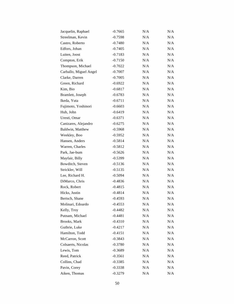
50
Jacquelin, Raphael -0.7665 N/A N/A Streelman, Kevin -0.7598 N/A N/A Castro, Roberto -0.7480 N/A N/A Edfors, Johan -0.7405 N/A N/A Luiten, Joost -0.7183 N/A N/A Compton, Erik -0.7150 N/A N/A Thompson, Michael -0.7022 N/A N/A Carballo, Miguel Angel -0.7007 N/A N/A Clarke, Darren -0.7005 N/A N/A Green, Richard -0.6922 N/A N/A Kim, Bio -0.6817 N/A N/A Bramlett, Joseph -0.6783 N/A N/A Ikeda, Yuta -0.6711 N/A N/A Fujimoto, Yoshinori -0.6603 N/A N/A Huh, John -0.6419 N/A N/A Uresti, Omar -0.6371 N/A N/A Canizares, Alejandro -0.6275 N/A N/A Baldwin, Matthew -0.5968 N/A N/A Weekley, Boo -0.5952 N/A N/A Hansen, Anders -0.5814 N/A N/A Warren, Charles -0.5812 N/A N/A Park, Jae-bum -0.5626 N/A N/A Mayfair, Billy -0.5399 N/A N/A Bowditch, Steven -0.5136 N/A N/A Strickler, Will -0.5135 N/A N/A Lee, Richard H. -0.5094 N/A N/A DiMarco, Chris -0.4836 N/A N/A Rock, Robert -0.4815 N/A N/A Hicks, Justin -0.4814 N/A N/A Bertsch, Shane -0.4593 N/A N/A Molinari, Edoardo -0.4553 N/A N/A Kelly, Troy -0.4482 N/A N/A Putnam, Michael -0.4481 N/A N/A Brooks, Mark -0.4310 N/A N/A Guthrie, Luke -0.4217 N/A N/A Hamilton, Todd -0.4151 N/A N/A McCarron, Scott -0.3843 N/A N/A Colsaerts, Nicolas -0.3780 N/A N/A Lewis, Tom -0.3689 N/A N/A Reed, Patrick -0.3561 N/A N/A Collins, Chad -0.3385 N/A N/A Pavin, Corey -0.3338 N/A N/A Aiken, Thomas -0.3279 N/A N/A
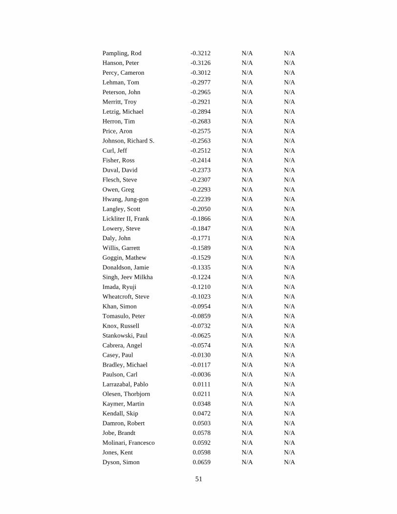
51
Pampling, Rod -0.3212 N/A N/A Hanson, Peter -0.3126 N/A N/A Percy, Cameron -0.3012 N/A N/A Lehman, Tom -0.2977 N/A N/A Peterson, John -0.2965 N/A N/A Merritt, Troy -0.2921 N/A N/A Letzig, Michael -0.2894 N/A N/A Herron, Tim -0.2683 N/A N/A Price, Aron -0.2575 N/A N/A Johnson, Richard S. -0.2563 N/A N/A Curl, Jeff -0.2512 N/A N/A Fisher, Ross -0.2414 N/A N/A Duval, David -0.2373 N/A N/A Flesch, Steve -0.2307 N/A N/A Owen, Greg -0.2293 N/A N/A Hwang, Jung-gon -0.2239 N/A N/A Langley, Scott -0.2050 N/A N/A Lickliter II, Frank -0.1866 N/A N/A Lowery, Steve -0.1847 N/A N/A Daly, John -0.1771 N/A N/A Willis, Garrett -0.1589 N/A N/A Goggin, Mathew -0.1529 N/A N/A Donaldson, Jamie -0.1335 N/A N/A Singh, Jeev Milkha -0.1224 N/A N/A Imada, Ryuji -0.1210 N/A N/A Wheatcroft, Steve -0.1023 N/A N/A Khan, Simon -0.0954 N/A N/A Tomasulo, Peter -0.0859 N/A N/A Knox, Russell -0.0732 N/A N/A Stankowski, Paul -0.0625 N/A N/A Cabrera, Angel -0.0574 N/A N/A Casey, Paul -0.0130 N/A N/A Bradley, Michael -0.0117 N/A N/A Paulson, Carl -0.0036 N/A N/A Larrazabal, Pablo 0.0111 N/A N/A Olesen, Thorbjorn 0.0211 N/A N/A Kaymer, Martin 0.0348 N/A N/A Kendall, Skip 0.0472 N/A N/A Damron, Robert 0.0503 N/A N/A Jobe, Brandt 0.0578 N/A N/A Molinari, Francesco 0.0592 N/A N/A Jones, Kent 0.0598 N/A N/A Dyson, Simon 0.0659 N/A N/A
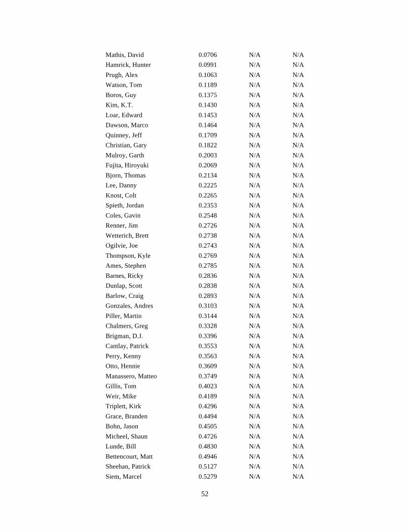
52
Mathis, David 0.0706 N/A N/A Hamrick, Hunter 0.0991 N/A N/A Prugh, Alex 0.1063 N/A N/A Watson, Tom 0.1189 N/A N/A Boros, Guy 0.1375 N/A N/A Kim, K.T. 0.1430 N/A N/A Loar, Edward 0.1453 N/A N/A Dawson, Marco 0.1464 N/A N/A Quinney, Jeff 0.1709 N/A N/A Christian, Gary 0.1822 N/A N/A Mulroy, Garth 0.2003 N/A N/A Fujita, Hiroyuki 0.2069 N/A N/A Bjorn, Thomas 0.2134 N/A N/A Lee, Danny 0.2225 N/A N/A Knost, Colt 0.2265 N/A N/A Spieth, Jordan 0.2353 N/A N/A Coles, Gavin 0.2548 N/A N/A Renner, Jim 0.2726 N/A N/A Wetterich, Brett 0.2738 N/A N/A Ogilvie, Joe 0.2743 N/A N/A Thompson, Kyle 0.2769 N/A N/A Ames, Stephen 0.2785 N/A N/A Barnes, Ricky 0.2836 N/A N/A Dunlap, Scott 0.2838 N/A N/A Barlow, Craig 0.2893 N/A N/A Gonzales, Andres 0.3103 N/A N/A Piller, Martin 0.3144 N/A N/A Chalmers, Greg 0.3328 N/A N/A Brigman, D.J. 0.3396 N/A N/A Cantlay, Patrick 0.3553 N/A N/A Perry, Kenny 0.3563 N/A N/A Otto, Hennie 0.3609 N/A N/A Manassero, Matteo 0.3749 N/A N/A Gillis, Tom 0.4023 N/A N/A Weir, Mike 0.4189 N/A N/A Triplett, Kirk 0.4296 N/A N/A Grace, Branden 0.4494 N/A N/A Bohn, Jason 0.4505 N/A N/A Micheel, Shaun 0.4726 N/A N/A Lunde, Bill 0.4830 N/A N/A Bettencourt, Matt 0.4946 N/A N/A Sheehan, Patrick 0.5127 N/A N/A Siem, Marcel 0.5279 N/A N/A

53
Martin, Ben 0.5305 N/A N/A Cejka, Alex 0.5459 N/A N/A Couples, Fred 0.5975 N/A N/A Elkington, Steve 0.6038 N/A N/A Allen, Michael 0.6096 N/A N/A Gutschewski, Scott 0.6149 N/A N/A Small, Mike 0.6190 N/A N/A Randolph, Jonathan 0.6222 N/A N/A Herman, Jim 0.6280 N/A N/A Uihlein, Peter 0.6305 N/A N/A Olazabal, Jose Maria 0.6313 N/A N/A Hayes, J.P. 0.6321 N/A N/A Hurley III, Billy 0.6546 N/A N/A Weibring, Matt 0.6643 N/A N/A Lawrie, Paul 0.6657 N/A N/A Purdy, Ted 0.6716 N/A N/A Sutherland, Kevin 0.6767 N/A N/A Lonard, Peter 0.6802 N/A N/A Noren, Alexander 0.7038 N/A N/A Waldorf, Duffy 0.7047 N/A N/A Matsuyama, Hideki 0.7127 N/A N/A Calcavecchia, Mark 0.7344 N/A N/A Fdez-Castano, Gonzalo 0.7371 N/A N/A Stolz, Andre 0.7409 N/A N/A Miller, Zack 0.7432 N/A N/A Wilson, Dean 0.7441 N/A N/A Sim, Michael 0.7511 N/A N/A Cabrera Bello, Rafael 0.7559 N/A N/A Gamez, Robert 0.7722 N/A N/A Gronberg, Mathias 0.7766 N/A N/A Kuehne, Hank 0.7861 N/A N/A Pagunsan, Juvic 0.7868 N/A N/A Muto, Toshinori 0.7887 N/A N/A Kokrak, Jason 0.7902 N/A N/A Reifers, Kyle 0.7906 N/A N/A Jimenez, Miguel A. 0.7991 N/A N/A Quiros, Alvaro 0.8004 N/A N/A Gore, Jason 0.8134 N/A N/A Gordon, Scott 0.8152 N/A N/A Todd, Brendon 0.8250 N/A N/A Lovemark, Jamie 0.8394 N/A N/A Kraft, Kelly 0.8514 N/A N/A Yang, Y.E. 0.8538 N/A N/A
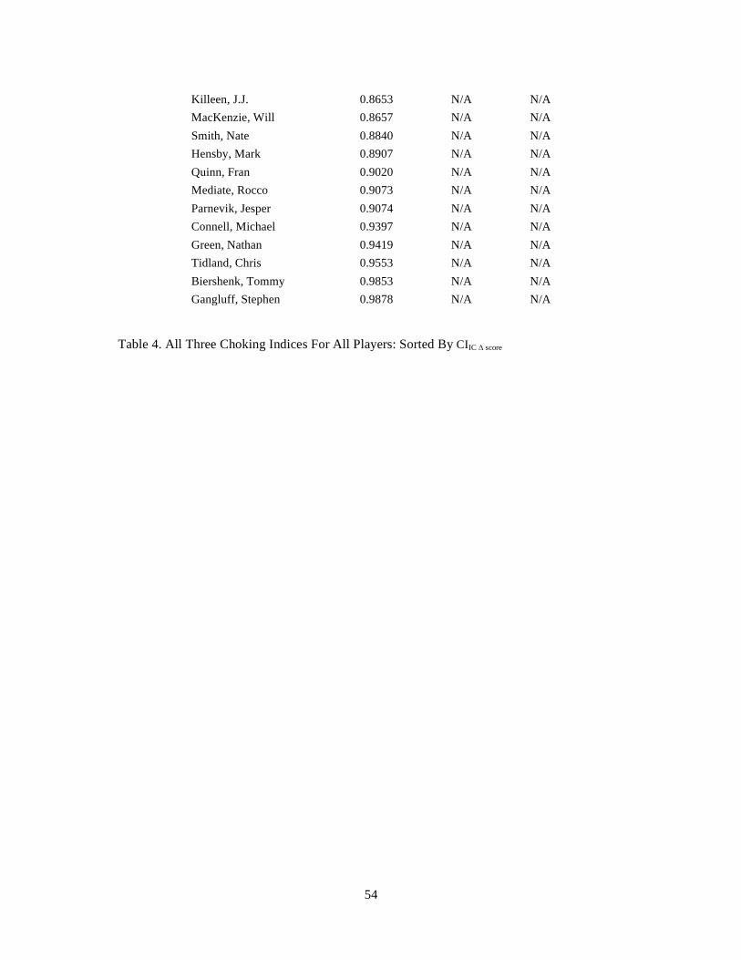
54
Killeen, J.J. 0.8653 N/A N/A MacKenzie, Will 0.8657 N/A N/A Smith, Nate 0.8840 N/A N/A Hensby, Mark 0.8907 N/A N/A Quinn, Fran 0.9020 N/A N/A Mediate, Rocco 0.9073 N/A N/A Parnevik, Jesper 0.9074 N/A N/A Connell, Michael 0.9397 N/A N/A Green, Nathan 0.9419 N/A N/A Tidland, Chris 0.9553 N/A N/A Biershenk, Tommy 0.9853 N/A N/A Gangluff, Stephen 0.9878 N/A N/A
Table 4. All Three Choking Indices For All Players: Sorted By CIIC Δ score

55
REFERENCES
[1] Baumeister, R. F, Choking under pressure: Self-consciousness and paradoxical effects of
incentives on skillful performance, Journal of Personality and Social Psychology, 1984, Vol 16:
610–620.
[2] Otten, Mark, Choking vs. Clutch Performance: A Study of Sport Performance Under
Pressure, Journal of Sport and Exercise Psychology, 2009, Vol. 31: 583-601.
[3] Harms, William, Psychologist Shows Why We “Choke” Under Pressure – And How To Avoid
It, The University of Chicago News, Sept. 2010,
<http://news.uchicago.edu/article/2010/09/21/psychologist-shows-why-we-choke-under-pressure-
and-how-avoid-it>.
[4] Syed, Matthew, The Psychology of Choking, BBC Sport, April 2011,
<http://www.bbc.co.uk/sport/0/13185266>.
[5] Click, James, et al, Baseball Between the Numbers: Why Everything You Know about the
Game is Wrong, Basic Books: New York, 2006, 14-16.
[6] PGA Tour, Inc, ShotLink Data, <http://stats.pgatourhq.com>.
[7] Miller, Irwin and Marylees Miller, John E. Freund Mathematical Statistics, 6th Ed, Prentice
Hall, 1999.
[8] Smith, Martha K., Type I and II Errors and Significance Levels, May 2011,
<http://www.ma.utexas.edu/users/mks/statmistakes/errortypes.html>.
[9] Ruxton, Graeme D., The unequal variance t-test is an underused alternative to Student's t-test
and the Mann–Whitney U test, Behavioral Ecology, July/Aug. 2006, Vol. 17.4: 688-690.
[10] Welch, B. L., The Generalization of `Student's' Problem when Several Different Population
Variances are Involved, Biometrika, Jan 1947, Vol. 34.1: 28-35.
[11] The MathWorks, Inc, Noncentral T Distribution, 2013,
<http://www.mathworks.com/help/stats/noncentral-t-distribution.html>.
56
[12] Sdorow, Lester, Psychology, 4th Ed, McGraw-Hill: New York, 1998, 394-395.
[13] Diamond, DM, et al, The Temporal Dynamics Model of Emotional Memory Processing: A
Synthesis on the Neurobiological Basis of Stress-Induced Amnesia, Flashbulb and Traumatic
Memories, and the Yerkes-Dodson Law, Neural Plasticity, 2007, 33.