the chebotar¨ev density theorem applications · for solving some cubic equations. in ad 1500 a...
TRANSCRIPT
UNIVERSITA DEGLI STUDI ROMA TREFACOLTA DI SCIENZE MATEMATICHE FISICHE NATURALI
Graduation Thesis in Mathematics
by
Alfonso Pesiri
The Chebotarev Density
Theorem
Applications
Supervisor
Prof. Francesco Pappalardi
The Candidate The Supervisor
ACADEMIC YEAR 2006 - 2007
OCTOBER 2007
AMS Classification: primary 11R44; 12F10; secondary 11R45; 12F12.
Key Words: Chebotarev Density Theorem, Galois theory, Transitive groups.
Contents
Introduction . . . . . . . . . . . . . . . . . . . . . . . . . . . . . . . 1
1 Algebraic background 10
1.1 The Frobenius Map . . . . . . . . . . . . . . . . . . . . . . . . 10
1.2 The Artin Symbol in Abelian Extensions . . . . . . . . . . . . 12
1.3 Quadratic Reciprocity . . . . . . . . . . . . . . . . . . . . . . 17
1.4 Cyclotomic Extensions . . . . . . . . . . . . . . . . . . . . . . 20
1.5 Dedekind Domains . . . . . . . . . . . . . . . . . . . . . . . . 22
1.6 The Frobenius Element . . . . . . . . . . . . . . . . . . . . . . 26
2 Chebotarev’s Density Theorem 32
2.1 Symmetric Polynomials . . . . . . . . . . . . . . . . . . . . . . 32
2.2 Dedekind’s Theorem . . . . . . . . . . . . . . . . . . . . . . . 33
2.3 Frobenius’s Theorem . . . . . . . . . . . . . . . . . . . . . . . 36
2.4 Chebotarev’s Theorem . . . . . . . . . . . . . . . . . . . . . . 39
2.5 Frobenius and Chebotarev . . . . . . . . . . . . . . . . . . . . 40
2.6 Dirichlet’s Theorem on Primes in Arithmetic Progression . . . 41
2.7 Hint of the Proof . . . . . . . . . . . . . . . . . . . . . . . . . 46
3 Applications 48
3.1 Charming Consequences . . . . . . . . . . . . . . . . . . . . . 48
3.2 Primes and Quadratic Forms . . . . . . . . . . . . . . . . . . . 52
3.3 A Probabilistic Approach . . . . . . . . . . . . . . . . . . . . . 55
3.4 Transitive Groups . . . . . . . . . . . . . . . . . . . . . . . . . 61
1
4 Inverse Galois Problem 71
4.1 Computing Galois Groups . . . . . . . . . . . . . . . . . . . . 71
4.2 Groups of Prime Degree Polynomials . . . . . . . . . . . . . . 83
A Roots on Finite Fields 88
B Galois Groups on Finite Fields 90
C The Chebotarev Test in Maple 92
Bibliography 113
2
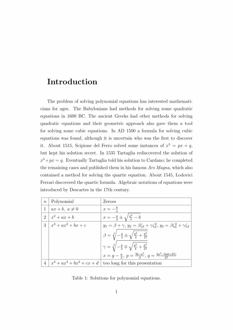
Introduction
The problem of solving polynomial equations has interested mathemati-
cians for ages. The Babylonians had methods for solving some quadratic
equations in 1600 BC. The ancient Greeks had other methods for solving
quadratic equations and their geometric approach also gave them a tool
for solving some cubic equations. In AD 1500 a formula for solving cubic
equations was found, although it is uncertain who was the first to discover
it. About 1515, Scipione del Ferro solved some instances of x3 = px + q,
but kept his solution secret. In 1535 Tartaglia rediscovered the solution of
x3 +px = q. Eventually Tartaglia told his solution to Cardano; he completed
the remaining cases and published them in his famous Ars Magna, which also
contained a method for solving the quartic equation. About 1545, Lodovici
Ferrari discovered the quartic formula. Algebraic notations of equations were
introduced by Descartes in the 17th century.
n Polynomial Zeroes
1 ax + b, a 6= 0 x = − ba
2 x2 + ax + b x = −a2±√
a2
4− b
3 x3 + ax2 + bx + c y1 = β + γ, y2 = βζ3 + γζ23 , y3 = βζ2
3 + γζ3
β =3
√− q
2±√
q2
4+ p3
27
γ =3
√− q
2∓√
q2
4+ p3
27
x = y − a3, p = 3b−a2
3, q = 2a3−9ab+27c
27
4 x4 + ax3 + bx2 + cx + d too long for this presentation
Table 1: Solutions for polynomial equations.
1

Since it was now possible to solve all polynomial equations of degree ≤ 4
by radicals, the next problem was how to solve the quintic equation. In 1770
Lagrange proved that the tricks used to solve equations of a lower degree do
not work for the quintic. This arose the suspicion that the quintic equation
may not be always solvable by radicals. The first person to publish a proof
for this was Ruffini. He made a first attempt in 1799 in his book Teoria
Generale delle Equazioni and then tried again with a better, but still not
accurate, proof in a journal in 1813. In 1824 Abel filled the gap in Ruffini’s
proof. Actually, neither the proof of Ruffini nor that of Abel is correct in
details, but Abel’s proof was accepted by his contemporaries and Ruffini’s
was not. Kronecker published in 1879 a simpler proof that there is no formula
for solving all quintic equations by radicals. This led to a new question: how
can we see if a special equation can be solved by radicals? In 1843 Liouville
wrote to the Academy of Science in Paris that, among the papers of the late
Galois, he had found a proof that the quintic is insoluble by radicals: this
was the origin of the Galois theory.
The problem of determining the Galois group of a polynomial from its
coefficients has held the interest of mathematicians for over a hundred years.
There is a classical algorithm for determining the Galois group of a poly-
nomial from its roots which can be found in Section 2.2, but the method is
cumbersome and is not of much interest from a practical point of view. More
recently Richard Stauduhar has applied modern insights to old techniques,
to develop and implement a computer algorithm that finds Galois groups of
low degree polynomials with integer coefficients, as explained in [Sta73]. We
will follow a different way, based fundamentally on a technical but powerfull
theorem in Algebraic Number Theory: the Chebotarev Density Theorem.
This theorem is due to the Russian mathematician Nikolai Grigor’evich Cheb-
otarev, who made his discovery in 1922, as he recalls in a letter of 1945:
I belong to the old generation of Soviet scientists, who were
shaped by the circumstances of a civil war. I devised my best re-
sult while carrying water from the lower part of town (Peresypi in
2
Odessa) to the higher part, or buckets of cabbages to the market,
which my mother sold to feed the entire family.
To describe Chebotarev’s theorem, let us denote with L/K a finite Galois
extension of algebraic number fields with group G. For each prime ideal
p ∈ K which is unramified in L, let σp denote its Frobenius element. Then
the Dirichlet density of the set of prime ideals with a given Frobenius element
C exists and equals |C|/|G|.The construction of the Frobenius element is mildly technical, which forms
the main cause for the relative unpopularity of Chebotarev’s theorem outside
Algebraic Number Theory.
In Chapter 1 we introduce the algebraic knowledges necessary to under-
stand the Frobenius element. We can characterize this element in the abelian
case with the following.
Theorem 1.2.1. Let f(x) ∈ Z[x] be an irreducible polynomial such that
Gal(f) = Gal(Q[α]/Q) is abelian, and p be a prime number not dividing
∆(f). Then there is a unique element ϕp ∈ Gal(f) such that the Frobenius
map of the ring Fp[α] is the reduction of ϕp modulo p; this means that, in
the ring Q[α], one has
αp = ϕp(α) + p · (q0 + q1α + · · ·+ qn−1αn−1)
for certain rational numbers q0, . . . , qn−1 of which the denominators are not
divisible by p.
We start considering minimal abelian extensions of K = Q. Elemen-
tary considerations in the case of a quadratic extension Q(√
D), where D is
square–free, lead us to a very explicit description of the fact: if we identify
Gal(Q(√
D)/Q) with the multiplicative group of two elements ±1, then
ϕp turns out to be the Legendre symbol(
Dp
). Another easy case is the
cyclotomic one: in this situation σp is the element of Gal(L/Q) such that
σ(ζn) = ζpn. In fact, modulo p we have
σ(∑
aiζin
)=∑
aiζipn =
∑ap
i ζipn =
(∑aiζ
in
)p
3
as required. Therefore, if we identify Gal(Φm) with (Z/mZ)∗, the Frobenius
element of a prime ideal p = pZ is simply given by p mod m.
Thus the Frobenius element of a prime ideal p ∈ OK is always an element of
Gal(L/K), where L is the splitting field of f(x) ∈ K[x]. It’s interesting to
notice that the degree of each irreducible factor of the polynomial (f mod p)
in Fp[x] is equal to the order of ϕp in the group G. In particular, one has
ϕp = id in G if and only if (f mod p) splits into n linear factors in Fp[x].
This will be fundamental in order to relate the Chebotarev theorem to the
computation of Galois groups.
A general discussion on the Frobenius element put us inside the theory
of Dedekind Domains. The notions of Decomposition group
G(P) := σ ∈ G s.t. σP = P
of a prime ideal P ∈ OL s.t. P|p lead us to the following definition.
Definition 1.6.5. We define the Frobenius element σP = (P, L/K) of P
to be the element of G(P) that acts as the Frobenius automorphism on the
residue field extension FP/Fp.
Even if it’s a general characterization, it does not give information about
a constructive method for the computation of the Frobenius element.
In Chapter 2 we explore three theorems which can be regarded as par-
ticular case of the main theorem. Finally we state a reformulation of the
Chebotarev Density theorem.
Theorem 2.5.1 Let f(x) ∈ Z[x] be a monic polynomial. Assume that the
discriminant ∆(f) of f(x) does not vanish. Let C be a conjugacy class of
the Galois group G = Gal(f). Then the set of primes p not dividing ∆(f)
for which σp belongs to C has a density, and this density equals |C|/|G|.Since the cycle pattern of σp ∈ Gal(f), with p = pZ, equals the decompo-
sition type of f mod p, the above theorem implies the following, sometimes
called Dedekind’s Theorem.
Corollary 2.2.4. Let f(x) ∈ Z[x] be a monic polynomial of degree m,
4
and let p be a prime number such that (f mod p) has simple roots, that is
p - ∆(f). Suppose that (f mod p) =∏
fi, with fi irreducible of degree mi
in Fp[x]. Then Gal(f) contains an element whose cycle decomposition is of
type m = m1 + · · ·+ mr.
The above result give the following strategy for computing the Galois
group of an irreducible polynomial f ∈ Z[x]. Factor f modulo a sequence
of primes p not dividing ∆(f) to determine the cycle types of the elements
in Gal(f); continue until a sequence of prime numbers has yielded no new
cycle types for the elements. Then attempt to read off the type of the group
from tables of transitive groups of degree ∂f . To make the computation more
effective, in a technical sense, we need the Frobenius Theorem.
Theorem 2.3.1. The density of the set of prime p for which f(x) has a
given decomposition type n1, n2, · · · , ni, exists, and it is equal to 1/#Gal(f)
times the number of σ ∈ G with decomposition in disjoint cycle of the form
cn1cn2 · · · cni, where cnk
is a nk–cycle.
The Frobenius Density Theorem, which Chebotarev generalizes, says that
if a cycle type occurs in Gal(f), then this will be seen by looking modulo a
set of prime numbers of positive density. To compute Gal(f), look up a table
of transitive subgroups of Sn with order divisible by n and their cycle types
distribution. We will see that this strategy is not always effective, and other
tools are needed.
The Frobenius Density Theorem is a specialization of the main theorem in
which C is required to be a division of G rather than a conjugacy class;
here we say that two elements of G belong to the same division if the cyclic
subgroups that they generate are conjugate in G. The partition of G into
divisions is, in general, less fine than its partition into conjugacy classes and
Frobenius’s theorem is correspondingly weaker than Chebotarev’s.
Last theorem discussed is the celebrated Dirichlet’s Theorem on Primes
in Arithmetic Progression.
Theorem 2.6.1. For each pair of integers a, m such that gcd(a, m) = 1, the
set S of prime numbers p such that p ≡ a mod m has density 1/ϕ(m), where
5
ϕ is the classical Euler function.
It’s an easy consequence of the main theorem, based on the fact that
there is a bijective correspondence between the conjugacy classes modm of
prime numbers that do not divide m and the elements of the group Gal(Φm),
which is isomorphic to (Z/mZ)∗, given by the map p ↔ σp, so that we may
identify σp with p mod m, as explained in Chapter 1. Hence
δ (p ≡ a mod m) = δ (p s.t. σp : ζm 7→ ζam) =
1
ϕ(m).
This chapter ends with an elementary proof of Chebotarev’s theorem in the
quadratic case, based on the theory of congruences. Finally is given a more
extensive, but not general, proof which follows Chebotarev’s original strategy,
avoiding the technical Class Field Theory.
Chapter 3 deals with applications of the main theorem. The first one
is about polynomials which have a root modulo almost all primes, that is,
except for a finite number of primes.
Theorem 3.1.7. Let f(x) ∈ Z[x] be an irreducible polynomial that has a
zero modulo almost all primes p. Then f(x) is linear.
Next, we have an interesting result about primes p for which f mod p has
no zeros.
Theorem 3.1.1. Let f(x) ∈ Z[x] be an irreducible polynomial of degree
n > 1. If p is prime, let Np(f) be the number of zeros of f in Fp = Z/pZ.
Then there are infinitely many primes p such that Np(f) = 0. Moreover the
set P0(f) of p’s with Np(f) = 0 has a density c0 = c0(f) ≥ 1/n.
The proof is long but not difficult, an is based on Burneside’s Lemma.
A collateral consequence of this lemma is that the mean value of Np(f) for
p →∞ is equal to 1. In other words,∑p≤x
Np(f) ≈ π(x) when x →∞,
where π(x) = #p primes s.t. p ≤ x.The third argument is a classical theorem about primitive positive definite
6

quadratic forms ax2 +bxy+cy2 which represent prime numbers. We will just
consider particular cases, obtaining results of the type
δ(p ≥ 3 s.t. p = x2 + ny2) =1
2,
for all n such that the class number h(−4n) equals 1.
The rest of the Chapter takes care for illustrate how the Chebotarev theorem
can be combined with other tools in order to get a powerfull algorithm to
compute Galois groups of irreducible polynomials in Z[x]. The strategy is as
follows.
1. test whether f is irreducible over Z;
2. compute the discriminant ∆(f);
3. factor f modulo primes not dividing the discriminant until you seem
to be getting no new decomposition type;
4. compute the orbit lengths on the r–sets of roots;
5. use tables of transitive groups of degree ∂f .
If ∂f ≤ 7, then third point suggested by Chebotarev’s theorem is effective,
but for higher degrees, this test gets into problems. In fact it is possible to
construct two non–isomorphic groups which have transitive permutation rep-
resentations in which the number of elements with a given cycle structure is
the same for both groups. In this situation other tests, like the one suggested
at point 4, are relevant.
Point 5 requires the knowledge of transitive permutation groups, so in the
last section of the chapter we include tables for groups of degree 3, 4, 5, 6, 7
and 11, as well.
The aim of Chapter 4 is to analyze the Maple code, given in Appendix C,
based on the modulo p reductions test suggested by the Chebotarev theorem,
for polynomials of degree from 3 to 7, and 11.
7
We tabulate several outputs in order to give an idea of the accuracy of our
tests, which depends on the choice of the upper bound k representing the
size of prime numbers that we want to consider. If we increase k, on the one
hand our result will be more precise, on the other hand Maple will need more
time to produce the output.
The polynomials considered are those of the type f(x) = xn + 2 and those
in Table 4.1 and 4.2 with Galois group An.
Then we introduce a notion of relative error ε(G) = ε(G, k) of the test, which
measure the distance between the theoretical and the empirical result. From
the analysis of these errors we notice that
ε(G, 106) < 10−2 and ε(G, 103) < 10−1,
and, by induction, one may naively guess ε(103t) < 10−t, t ≥ 1, when
G = Gal(f). This observation indicates that k ≥ 103 usually is a good
bound for the Chebotarev test.
This tool allows us to make several experiments in finding polynomial with
a given Galois group. In our attempts, we ran the program for all the poly-
nomials in Table 4.1 and 4.2, partially taken from [SM85], in which each
transitive permutation group of degree from 3 to 7 and 11 is realised as a
Galois group over the rationals. The choice p ≤ k = 1000 gave always the
correct output.
The chapter goes on with a section on the computation of Galois groups
for polynomials of prime degree p. We develop an algorithm based on the
existence of non–real roots of a polynomial.
If a prime degree polynomial f(x) has r = 2s complex roots, then we know
that a permutation of the type (2)r2 is in its Galois group. Hence, the list of
possible Galois groups for f(x) is much shorter than in general. Knowledge
of r provides us a further information: from a theorem of Jordan, it follows
that if r is small enough with respect to the degree p of the polynomial, then
the Galois group is Ap or Sp. The specific statement follows as a theorem.
Theorem 4.2.2. Let f(x) ∈ Q[x] be an irreducible polynomial of prime
degree p ≥ 3 and r = 2s be the number of non–real roots of f(x). If s
8

satisfies
s(slogs + 2logs + 3) ≤ p
then Gal(f) = Ap, or Sp.
If we consider f(x) such that ∂f = p ≤ 29, no two groups have the
same cycle structure, and so the Galois group can be determined uniquely
by reduction modulo p for all polynomials of prime degree ≤ 29.
Combining the above results we have an algorithm for computing the Galois
group of prime degree polynomials with non–real roots.
begin
r:=Number Of Real Roots(f(x));
if p > N(r)
if D(f) is a square
Gal(f)=A_p;
else Gal(f) = S_p;
else Chebotarev test(f(x));
end;
We remark that while the Chebotarev test is difficult to execute from a
computational point of view, checking whether a polynomial has non–real
roots is very efficient since numerical methods can be used.
9
Chapter 1
Algebraic background
1.1 The Frobenius Map
Every field has a unique minimal subfield, the prime subfield, and this is
isomorphic either to Q or to Zp, where p is a prime number. The proof of
this fact is easy and can be found in [Rot95]. Correspondingly, we say that
the characteristic of the field is 0 or p. In a field of characteristic p we have
px = 0 for every element x, where as usual we write
px = (1 + 1 + · · ·+ 1)x
where there are p summands 1, and p is the smallest positive integer with
this property. In a field of characteristic zero, if nx = 0 for some non–zero
element x and integer n, then n = 0.
Theorem 1.1.1. Let p be a prime number and R be a commutative ring of
characteristic p. Then F : a 7→ ap is a ring homomorphism from R to itself.
Proof. Clearly F (a·b) = (a·b)p = ap ·bp = F (a)·F (b), for any a, b ∈ R. Then
F (a+b) = (a+b)p =∑p
k=0
(pk
)ap−k ·bk. Since p|
(pk
), for all k = 1, 2, . . . p−1,
we get F (a + b) = ap + bp = F (a) + F (b).
The map in Theorem 1.1.1 is called the Frobenius Map after Georg Fer-
dinand Frobenius, realized its importance in Algebraic Number Theory in
10
1880.
Now, our goal is answering the following question: which ring homomorphism
R → R is F , that is, does F have a more direct description than through
p–th powering? We study two cases in which this can be done. Throughout
we let p be a prime number. The simplest ring of characteristic p is the field
Fp = Z/pZ of integers modulo p. Since any element of Fp can be written
as 1 + 1 + . . . + 1, the only ring homomorphism Fp → Fp is the identity. In
particular the Frobenius map F : Fp → Fp is the identity. Looking at the
definition of F we see that this observation proves Fermat’s Little Theorem:
for any integer a one has ap ≡ a (mod p). Next we consider quadratic ex-
tensions of Fp. Let d be a non–zero integer, and let p be a prime number
not dividing 2d. We consider the ring Fp[√
d] the elements of which are by
definition the formal expressions u + v√
d, with u and v ranging over Fp. If
d is not a square modulo p, then no two of these expressions are considered
equal and, therefore, the number of elements of the ring equals p2. The ring
operations are the obvious ones suggested by the notation, that is, we define
(u + v√
d) + (u′ + v′√
d) = (u + u′) + (v + v′)√
d, (1.1)
(u + v√
(d) · (u′ + v′√
d) = (uu′ + vv′d) + (uv′ + vu′)√
d,
where d in vv′d is interpreted to be the element d (mod p) of Fp. It is
straightforward to show that with these operations Fp[√
d] is a ring of char-
acteristic p. Let us now apply the Frobenius map F to a typical element
u + v√
d. Using, in succession, the definition of F , the fact that it is a ring
homomorphism, Fermat’s little theorem, the defining relation (√
d)2 = d and
the fact that p is odd, we find
F (u + v√
d) = (u + v√
d)p = up + vp(√
d)p = u + vd(p−1)/2(√
d).
This leads us to investigate the value of d(p−1)/2 in Fp. Again, from Fermat’s
little theorem, we have
0 = dp − d = d · (d(p−1)/2 − 1) · (d(p−1)/2 + 1).
11
Since Fp is a field, one of the three factors d, (d(p−1)/2−1), (d(p−1)/2 +1) must
vanish. As p does not divide d it is exactly one of the last two. The quadratic
residue symbol(
dp
)distinguishes the two cases: for d(p−1)/2 = +1 in Fp we
put(
dp
)= +1, and for d(p−1)/2 = −1 we put
(dp
)= −1. The conclusion is
that the Frobenius map is one of the two obvious automorphisms of Fp[√
d]:
for(
dp
)= +1 it is the identity and for
(dp
)= −1 it is the map sending
u+v√
d to u−v√
d. The assignment u+v√
d 7→ u−v√
d is clearly reminiscent
of complex conjugation, and it defines an automorphism in far more general
circumstances involving square roots. For example, we may define a ring
Q[√
d] by simply replacing Fp with the field Q of rational numbers in the
above. The ring Q[√
d] is a field when d is not a perfect square, but whether
or not it is a field it has an identity automorphism as well as an automorphism
of order 2 that maps u + v√
d to u− v√
d. If we restrict to integral u and v,
and reduce modulo p, then one of these two automorphisms will give rise to
the Frobenius map of Fp[√
d].
1.2 The Artin Symbol in Abelian Extensions
We next consider the situation for higher degree extensions. Instead of
x2 − d we consider any non–zero polynomial f(x) ∈ Z[x] of positive degree
n and with leading coefficient 1. Instead of d 6= 0 we require that f have
no repeated factors or, equivalently, that its discriminant ∆(f) be nonzero.
Instead of Fp[√
d] for a prime number p, we consider the ring Fp[α] consisting
of all pn formal expressions
u0 + u1α + u2α2 + . . . + un−1α
n−1
with coefficients ui ∈ Fp, the ring operations being the natural ones with
f(α) = 0. Here the coefficients of f(x), which are integers, are interpreted
in Fp, as before. Formally, one may define Fp[α] to be the quotient ring
Fp[x]/f(x)Fp[x]. In the same manner, replacing Fp by Q we define the ring
Q[α]. It is a field if and only if f(x) is irreducible.
12

We now need to make an important assumption, which is automatic for
n ≤ 2, but not for n ≥ 3. Namely, instead of two automorphisms, we assume
that a finite abelian group G of ring automorphisms of Q[α] is given such
that we have an equality
f(x) =∏σ∈G
(x− σ(α))
of polynomials with coefficients in Q[α]. This is a serious restriction. For
example, in the important case that f(x) is irreducible it is equivalent to
Q[α] being a Galois extension of Q with an abelian Galois group. Just as in
the quadratic case, the Frobenius map of Fp[α] is for almost all p induced by
a unique element of the group G. The precise statement is as follows.
Theorem 1.2.1. Let f(x) ∈ Z[x] be an irreducible polynomial such that
Gal(f) = Gal(Q[α]/Q) is abelian, and p be a prime number not dividing
∆(f). Then there is a unique element ϕp ∈ Gal(f) such that the Frobenius
map of the ring Fp[α] is the reduction of ϕp modulo p; this means that, in
the ring Q[α], one has
αp = ϕp(α) + p · (q0 + q1α + · · ·+ qn−1αn−1)
for certain rational numbers q0, . . . , qn−1 of which the denominators are not
divisible by p.
Proof. Follows from the definition of the Frobenius element given in Sec-
tion 1.6 and from Proposition 1.6.2.
In all our examples, the condition on the denominators of the qi is satisfied
simply because the qi are integers, in which case αp and ϕp(α) are visibly
congruent modulo p. However, there are cases in which the coefficients of
ϕp(α) have a true denominator, so that the qi will have denominators as
well. Requiring the latter to be not divisible by p prevents us from picking
any ϕp ∈ G and just defining the qi by the equation in the theorem.
The element ϕp of G is referred to as the Artin symbol of p. In the case
n = 2 it is virtually identical to the Legendre symbol(
∆(f)p
). Note that for
13
f(x) = x2 − d we have ∆(f) = 4d so the condition that p does not divide
∆(f) is in this case equivalent to p not dividing 2d. We can now say that,
for the ring Fp[α] occurring in Theorem 1.2.1, knowing the Frobenius map
is equivalent to knowing the Artin symbol ϕp in the group G. The Artin
Reciprocity Law imposes strong restrictions on how ϕp varies over G as p
ranges over all prime numbers not dividing ∆(f) and in this way it helps us
in determining the Frobenius map. Let us consider an example to illustrate
it.
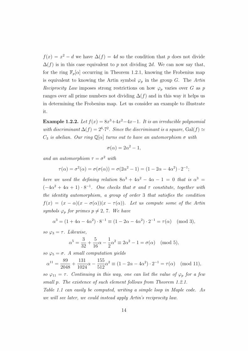
Example 1.2.2. Let f(x) = 8x3+4x2−4x−1. It is an irreducible polynomial
with discriminant ∆(f) = 26·72. Since the discriminant is a square, Gal(f) 'C3 is abelian. Our ring Q[α] turns out to have an automorphism σ with
σ(α) = 2α2 − 1,
and an automorphism τ = σ2 with
τ(α) = σ2(α) = σ(σ(α)) = σ(2α2 − 1) = (1− 2α− 4α2) · 2−1;
here we used the defining relation 8α3 + 4α2 − 4α − 1 = 0 that is α3 =
(−4α2 + 4α + 1) · 8−1. One checks that σ and τ constitute, together with
the identity automorphism, a group of order 3 that satisfies the condition
f(x) = (x − α)(x − σ(α))(x − τ(α)). Let us compute some of the Artin
symbols ϕp for primes p 6= 2, 7. We have
α3 = (1 + 4α− 4α2) · 8−1 ≡ (1− 2α− 4α2) · 2−1 = τ(α) (mod 3),
so ϕ3 = τ . Likewise,
α5 =3
32+
5
16α− 1
2α2 ≡ 2α2 − 1 = σ(α) (mod 5),
so ϕ5 = σ. A small computation yields
α11 =89
2048+
131
1024α− 155
512α2 ≡ (1− 2α− 4α2) · 2−1 = τ(α) (mod 11),
so ϕ11 = τ . Continuing in this way, one can list the value of ϕp for a few
small p. The existence of such element follows from Theorem 1.2.1.
Table 1.1 can easily be computed, writing a simple loop in Maple code. As
we will see later, we could instead apply Artin’s reciprocity law.
14
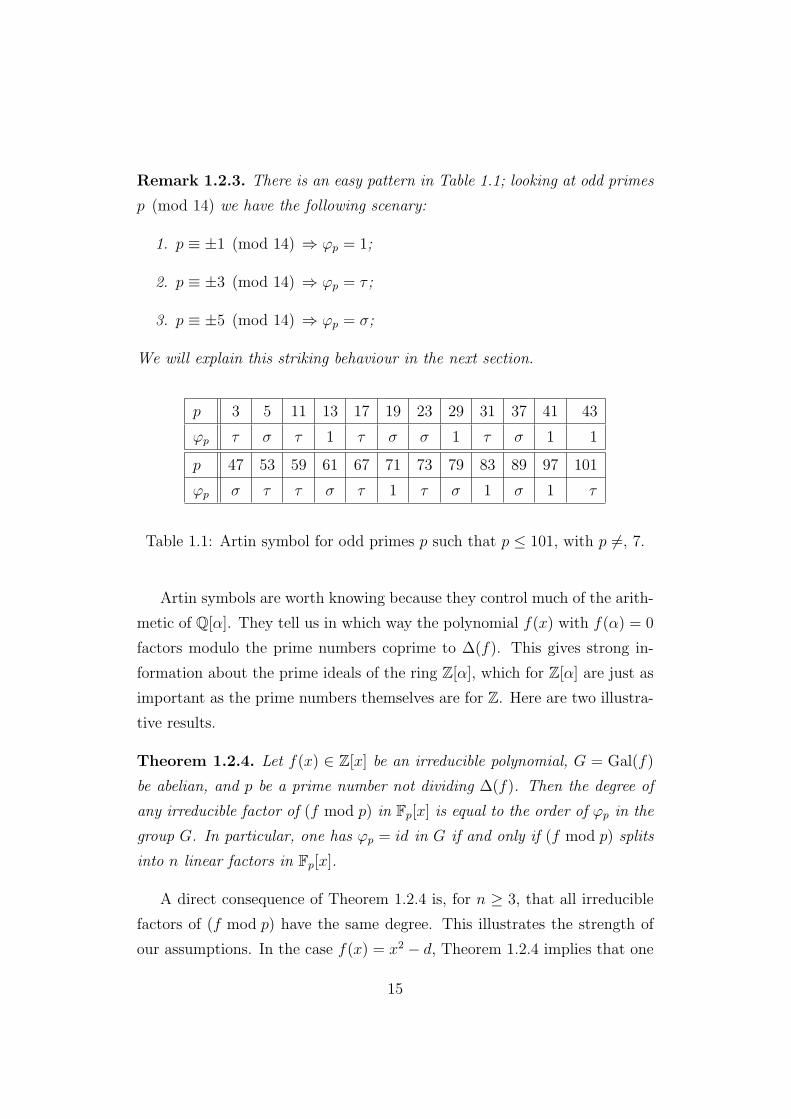
Remark 1.2.3. There is an easy pattern in Table 1.1; looking at odd primes
p (mod 14) we have the following scenary:
1. p ≡ ±1 (mod 14) ⇒ ϕp = 1;
2. p ≡ ±3 (mod 14) ⇒ ϕp = τ ;
3. p ≡ ±5 (mod 14) ⇒ ϕp = σ;
We will explain this striking behaviour in the next section.
p 3 5 11 13 17 19 23 29 31 37 41 43
ϕp τ σ τ 1 τ σ σ 1 τ σ 1 1
p 47 53 59 61 67 71 73 79 83 89 97 101
ϕp σ τ τ σ τ 1 τ σ 1 σ 1 τ
Table 1.1: Artin symbol for odd primes p such that p ≤ 101, with p 6=, 7.
Artin symbols are worth knowing because they control much of the arith-
metic of Q[α]. They tell us in which way the polynomial f(x) with f(α) = 0
factors modulo the prime numbers coprime to ∆(f). This gives strong in-
formation about the prime ideals of the ring Z[α], which for Z[α] are just as
important as the prime numbers themselves are for Z. Here are two illustra-
tive results.
Theorem 1.2.4. Let f(x) ∈ Z[x] be an irreducible polynomial, G = Gal(f)
be abelian, and p be a prime number not dividing ∆(f). Then the degree of
any irreducible factor of (f mod p) in Fp[x] is equal to the order of ϕp in the
group G. In particular, one has ϕp = id in G if and only if (f mod p) splits
into n linear factors in Fp[x].
A direct consequence of Theorem 1.2.4 is, for n ≥ 3, that all irreducible
factors of (f mod p) have the same degree. This illustrates the strength of
our assumptions. In the case f(x) = x2 − d, Theorem 1.2.4 implies that one
15

has(
dp
)= +1 if and only if d is congruent to a square modulo p. We give
a proof of the theorem above in the special case of cyclotomic polynomials.
The following result is taken from [LN94].
Theorem 1.2.5. Let Φn be the n–th cyclotomic polynomial and p be a prime
number coprime to n. Then (Φn mod p) splits in ϕ(n)/d distinct monic ir-
reducible polynomials in Fp[x] of the same degree d, where d is the minimum
positive integer such that pd ≡ 1 (mod n).
Proof. Let η be the n–th root of unity on Fp; then η ∈ Fpk ⇔ ηpk − η = 0,
that is ηpk= η, and so pk ≡ 1 (mod n). Now, let d be as in the statment;
pd ≡ 1 (mod n) ⇒ η ∈ Fpd , and @ F ⊂ Fpd such that η ∈ F. Hence the
minimum polynomial of η on Fp has degree d and, since η is an arbitrary
n–th root of unity, we have the statment.
Remark 1.2.6. In Section 1.4 we will see that, for a cyclotomic extension,
the Artin symbol is a tautology; ϕp maps ζn into ζpn, and therefore ord(ϕp) is
just the minimum positive integer d such that pd ≡ 1 (mod n).
Corollary 1.2.7. Let p be a prime number such that p ≡ 1 (mod n). Then
Φn splits into ∂Φn = ϕ(n) linear factor on Fp[x].
Example 1.2.8. Let f(x) = x4 + x3 + x2 + x + 1 be the 5–th cyclotomic
polynomial. Then we can determine the decomposition type of (f mod p) by
means of ϕp. If we identify Gal(f) = σj : a 7→ aj, for 1 ≤ j ≤ 4 with
(Z/5Z)∗, we have a very explicit description of the fact.
1. p ≡ 1 mod 5 ⇒ ϕp = σ1 ⇒ (f mod p) = (1)(1)(1)(1);
2. p ≡ 2 mod 5 ⇒ ϕp = σ2 ⇒ (f mod p) = (4);
3. p ≡ 3 mod 5 ⇒ ϕp = σ3 ⇒ (f mod p) = (4);
4. p ≡ 4 mod 5 ⇒ ϕp = σ4 ⇒ (f mod p) = (2)(2);
16

In general, the set of prime p such that f(x) splits modulo p can be de-
scribed by congruences conditions with respect to a modulus depending only
on f(x) if and only if Gal(f) is an abelian group. In fact, the non–abelian
case is more difficult to describe. For more details on this fact, see [Wym72].
1.3 Quadratic Reciprocity
To illustrate Artin’s reciprocity law, it is useful to go back to the quadratic
ring Q(√
d). In that case knowing ϕp is equivalent to knowing(
dp
), and
Artin’s reciprocity law is just a disguised version of the quadratic reciprocity
law. The latter states that for any two distinct odd prime numbers p and q
one has: (q
p
)=
(
pq
)if p ≡ 1 (mod 4)(
−pq
)if p ≡ 3 (mod 4)
The law is a theorem; it is the theorema fundamentale from Gauss’s Dis-
quisitiones arithmeticae (1801). Gauss also proved the supplementary laws(−1
p
)=
1 if p ≡ 1 (mod 4)
−1 if p ≡ 3 (mod 4)
and (2
p
)=
1 if p ≡ ±1 (mod 8)
−1 if p ≡ ±3 (mod 8)
The first one is immediate from the definition(d
p
)≡ d(p−1)/2 (mod p)
given in Section 1.1, also called Euler’s Criterion.
For our purposes it is more convenient to use a different formulation of the
quadratic reciprocity law. It goes back to Euler, who empirically discovered
the law in the 1740’s but was unable to prove it.
17
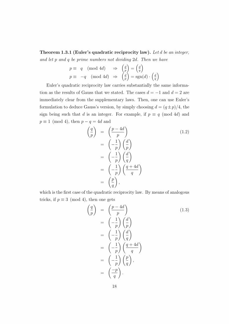
Theorem 1.3.1 (Euler’s quadratic reciprocity law). Let d be an integer,
and let p and q be prime numbers not dividing 2d. Then we have
p ≡ q (mod 4d) ⇒(
dp
)=(
dq
)p ≡ −q (mod 4d) ⇒
(dp
)= sgn(d) ·
(dq
)Euler’s quadratic reciprocity law carries substantially the same informa-
tion as the results of Gauss that we stated. The cases d = −1 and d = 2 are
immediately clear from the supplementary laws. Then, one can use Euler’s
formulation to deduce Gauss’s version, by simply choosing d = (q±p)/4, the
sign being such that d is an integer. For example, if p ≡ q (mod 4d) and
p ≡ 1 (mod 4), then p− q = 4d and(q
p
)=
(p− 4d
p
)(1.2)
=
(−1
p
)(d
p
)=
(−1
p
)(d
q
)=
(−1
p
)(q + 4d
q
)=
(p
q
),
which is the first case of the quadratic reciprocity law. By means of analogous
tricks, if p ≡ 3 (mod 4), then one gets(q
p
)=
(p− 4d
p
)(1.3)
=
(−1
p
)(d
p
)=
(−1
p
)(d
q
)=
(−1
p
)(q + 4d
q
)=
(−1
p
)(p
q
),
=
(−p
q
).
18

Not only did Euler observe that the value of the quadratic symbol(
dp
)depends only on (p mod 4d), he also noticed that
(dp
)exhibits multiplicative
properties as a function of p. For example, if p, q, j are primes satisfying
p ≡ qj (mod 4d), then we have(
dp
)=(
dq
)·(
dj
). Formulated in modern
language, this leads to a special case of Artin reciprocity. Denote, for a non–
zero integer m, by (Z/mZ)∗ the multiplicative group of invertible elements
of the ring Z/mZ. Let d again be any non–zero integer.
Theorem 1.3.2 (Artin quadratic reciprocity law). There exists a group
homomorphism
(Z/4dZ)∗ → ±1 (1.4)
(p mod 4d) 7→(
d
p
)for any prime p not dividing 4d.
If we wish to generalize Artin’s quadratic reciprocity law to higher degree
abelian polynomial it is natural to guess that 4d is to be replaced by ∆(f),
and(
dp
)by ϕp. This guess is correct. Let the polynomial f(x), the ring
Q[α], the abelian group G = Gal(f), and the Artin symbols ϕp for p not
dividing ∆(f) be as in Theorem 1.2.1.
Theorem 1.3.3 (Artin reciprocity law over Q). There exists a group
homomorphism
(Z/∆(f)Z)∗ → Gal(f)
(p mod ∆(f)) 7→ ϕp
for any prime number p not dividing ∆(f).
From Theorem 1.2.4 we know that ϕp determines the splitting behavior of
the polynomial f(x) modulo p, so Artin reciprocity yields a relation between
(f mod p) and (p mod ∆(f)).
In our cubic example f(x) = 8x3 + 4x2 − 4x− 1 we have ∆(f) = 26 · 72 and
19
G is of order 3. Thus, the reciprocity law implies that the Table 1.1 of Artin
symbols that we gave for f(x) is periodic with period dividing ∆(f), namely
with period 14 as we observed in Remark 1.2.3. It is a general phenomenon
for higher degree abelian extensions that the number ∆(f) in Theorem 1.3.3
can be replaced by a fairly small divisor.
Theorems 1.3.2 and 1.3.3 are simple reformulations of the Artin reciprocity
law. The original statement involves the notion of ray class group, which we
do not discuss in this work.
We state the law as formulated in [Wym72].
Theorem 1.3.4 (Artin Reciprocity Law). Let L/Q be a finite abelian
extension with Galois group G, and let Γ be the subgroup of Q∗ generated by
the primes unramified in L. Then the Artin symbol gives a surjective group
homomorphism
ϕ : Γ 7→ Gal(L/Q)
whose kernel contains the ray group Γa, where a is an appropriate product of
the ramified primes.
In theorems 1.3.2 and 1.3.3 we replace Γ with (Z/∆(f)Z)∗ so that we
express primes in terms of congruences modulo ∆(f), and, in this way, we
automatically exclude ramified primes. Moreover, this presentation gives an
explicit description of the Artin symbol ϕp just looking at (p mod ∆(f)).
1.4 Cyclotomic Extensions
Artin’s reciprocity law over Q generalizes the quadratic reciprocity law.
This generality depends on the study of cyclotomic extensions.
Let m be a positive integer, and define inductively the m–th cyclotomic
polynomial Φm(x) ∈ Z[x] to be the product
Φm(x) =xm − 1∏
d|m,d6=m Φd(x).
20

So one readly proves the identity∏d|m
Φd(x) = xm − 1,
from which we can derive that the degree of Φm equals ϕ(m) = #(Z/mZ)∗.
Therefore the discriminant ∆(Φm) divides the discriminant of ∆(xm − 1),
which equals ±mm. For example, the discriminant of Φ8(x) = x4 + 1, which
equals 28, divides ∆(x8− 1) = −224. Denoting by ζm a formal zero of Φm(x)
we obtain a ring Q[ζm] that has vector space dimension ϕ(m) over Q. We
have ζmm = 1, but ζd
m 6= 1 when d < m divides m, so the multiplicative order
of ζm equals m. In the polynomial ring over Q[ζm] the identity
Φm(x) =∏
a∈(Z/mZ)∗
(x− ζam)
is valid. One deduces that for each a ∈ (Z/mZ)∗ the ring Q[ζm] has an
automorphism φa : ζm 7→ ζam and that G = φa s.t. a ∈ (Z/mZ)∗ is a group
isomorphic to (Z/mZ)∗; in particular, it is abelian. This places us in the
situation of Theorem 1.2.1 with f = Φm and α = ζm. Applying the theorem,
we find ϕp = φp for all primes p not dividing m: all qi in the theorem vanish,
Artin’s reciprocity law is now almost a tautology. If we identify G with
(Z/mZ)∗, the Artin map
(Z/∆(Φm)Z) → (Z/mZ)∗
is simply the map
(a mod ∆(Φm)) 7→ (a mod m)
whenever a is coprime to m. This map is clearly surjective.
We conclude that for cyclotomic extensions, Artin’s reciprocity law can be
proved by means of a plain verification. One can now attempt to prove
Artin’s reciprocity law in other cases by reduction to the cyclotomic case. For
example, the supplementary law that gives the value of(
2p
)is a consequence
of the fact that ζ8 + ζ−18 is a square root of 2. Namely, one has
ϕp(√
2) = ϕp(ζ8 + ζ−18 ) ≡ (ζ8 + ζ−1
8 )p ≡ ζp8 + ζ−p
8 (mod p);
21

for p ≡ ±1 (mod 8), this equals
ζ8 + ζ−18 =
√2,
and for p ≡ ±3 (mod 8) it is
ζ38 + ζ−3
8 = ζ48 · (ζ8 + ζ−1
8 ) = −√
2.
This confirms that in the two respective cases one has(
2p
)= 1 and
(2p
)=
−1. Our example f(x) = 8x3 + 4x2 − 4x − 1 can also be reduced to the
cyclotomic case: if ζ14 is a zero of Φ14 then a computation shows that
α = (ζ214 + ζ−2
14 )/2 = (ζ214 − ζ5
14)/2
is a zero of f , and one finds
ϕp(α) = (ζ2p14 + ζ−2p
14 )/2 = (ζ2p14 − ζ5p
14 )/2.
As consequence of this fact, by more simple computations we have
ϕp(α) ≡
(ζ2
14 − ζ514)/2 = α for p ≡ ±1 (mod 14),
(−1− ζ214 + ζ3
14 − ζ414 + ζ5
14)/2 = τ(α) for p ≡ ±3 (mod 14),
(ζ414 − ζ3
14)/2 = σ(α) for p ≡ ±5 (mod 14).
This proves our remark on the pattern underlying the Table 1.1 of Artin
symbols. The theorem of Kronecker–Weber (1887) implies that the reduc-
tion to cyclotomic extensions will always be successful: this theorem asserts
that every abelian Galois extension of Q can be embedded in a cyclotomic
extension. That takes care of the case in which f(x) is irreducible, from
which the general case follows easily. In particular, to prove the quadratic
reciprocity law it suffices to express square roots of integers in terms of roots
of unity, as we just did with√
2.
1.5 Dedekind Domains
In the previous sections we gave an explicit description of the Artin sym-
bol relative to a prime number just in terms of congruences, that is, exploiting
22
informations based on Artin reciprocity. Here we provide an overview of the
general construction of the Artin symbol, which is a fundamental tool in
order to understand the Chebotarev Theorem. We put ourselves in a more
general contest, that is, the one of Dedekind Domains. The basic theory on
Dedekind Domains, which we take for granted, can be found in [ST02].
Definition 1.5.1. A Dedekind Domain A is a ring that satisfies the following
properties:
(a) A is a domain, with field of fractions K;
(b) A is noetherian, that is, every ideal in A is finitely generated;
(c) A is such that if α satisfies a monic polynomial equation with coefficients
in A then α ∈ A;
(d) every non–zero prime ideal of A is maximal.
In this section we will use the following notations: we denote by A a
Dedekind domain with field of fractions K, and with B the integral closure
of A in a finite separable extension L of K. It will be useful to think of the
simplest example for which these relations hold, namely A = Z, K = Q, B =
OL, where OL is the set of elements of L whose monic minimum polynomial
has coefficients in Z; this set make up the ring of algebraic integers in L. The
ring OL is a Dedekind domain when L/K is a finite extension of the number
field K. We recall the notion of division between ideals.
Definition 1.5.2. For ideals a, b of A, we say that
a|b ⇔ a ⊇ b.
Let p be a nonzero prime ideal of A. Then pB is an ideal of B, and it
has a factorization
pB = Pe11 Pe2
2 · · ·Pegg , ei > 0,
where P1, . . . ,Pg are distinct prime ideals of B, and e1, . . . , eg are positive
integers. Hence P divides p, written P | p, if P occurs in the factorization
of pB. Primes dividing p have a specific property.
23
Lemma 1.5.3. A prime ideal P of B divides p if and only if p = P ∩ A.
Proof. (⇒) Clearly p ⊂ P∩A; but P∩A 6= A and p is maximal, so P∩A = p.
(⇐) If p ⊂ P then pB ⊂ P, and this implies that P occurs in the factoriza-
tion of pB.
Definition 1.5.4. If any of the numbers ei is > 1, then we say that p is
ramified in B; the number ei = e(Pi/p) is called the ramification index. We
then write fi = f(Pi/p) for the vector space dimension [B/Pi : A/p], called
the relative degree of Pi.
Example 1.5.5. Let L = Q[√
2] and K = Q; it follows that B = Z[√
2] and
A = Z. The prime ideal (2) = 2Z has the factorization 2B = (√
2B)2. It’s
easy to see that√
2B is a prime ideal because
√2B = 2Z +
√2Z,
and so B/√
2B is the field of 2 elements. It follows that the ramification index
e(P/(2)) of P =√
2B is 2, and f(P/(2)) is [Z[√
2]/√
2Z[√
2] : Z/2Z] = 1,
since they are both isomorphic to a field of 2 elements. Thus the prime ideal
(2) = 2Z ramifies in B = Z[√
2].
Lemma 1.5.6. Let L/K be a finite Galois extension and G = Gal(L/K).
Let p be a prime ideal of OK and let P1, P2 be prime ideals of OL dividing
p. Then there exists σ ∈ G such that P1 = σ(P2).
Proof. Suppose that P1 6= σ(P2), ∀σ ∈ G. By the Chinese Reminder The-
orem, there exists an element x ∈ B such that x ≡ 0 (mod P1), and
x ≡ 1 mod σ(P2),∀σ ∈ G. The element
N(x) :=∏σ∈G
σ(x)
lies in B ∩ K = A, and lies in P1 ∩ A = p, because P1 | p. But x 6∈σ(P2),∀σ ∈ G, so that σ(x) 6∈ P2,∀σ ∈ G. This contradicts the fact that
N(x) lies in p = P2 ∩ A.
24

Theorem 1.5.7. Let m be the degree of the field extension L/K, and let
P1, . . . ,Pg be the prime ideals dividing p; then
g∑i=1
eifi = m.
Moreover, if L/K is a Galois extension, then all the ramification numbers
and all the relative degrees are equal; therefore
efg = m.
Proof. See [Sam67, Chap.5]. The proof of the equality in the case of abelian
extensions follows from Lemma 1.5.6.
Definition 1.5.8. Let L be a finite extension of degree m over K = Q,
and α1, . . . , αm be a basis of L as vector space over Q. We define the
discriminant of this basis to be
∆[α1, . . . , αn] = det[σi(αj)]2, i, j = 1, . . . m,
for all σi : L → C such that σi is a K–homomorphism.
We will focus on basis for OL over OK = Z, called an integral basis for
OL. If α1, . . . , αm if an integral basis for OL, then we can prove that
∆[α1, . . . , αn] is a rational integer and that if β1, . . . , βn is another integral
basis for OL, then ∆[β1, . . . , βn] = ∆[α1, . . . , αn]. For the proof of these facts,
see [ST02, Chap.2].
The following gives a description of the prime ideals that ramify in an exten-
sion.
Theorem 1.5.9. A prime ideal p = pZ ∈ OK = Z ramifies in OL if and only
if p | ∆(OL/Z). In particular, only finitely many prime ideals ramify.
Proof. See [Sam67, Chap.5].
In other words, a prime ideal p ∈ Z ramifies in OL if and only if p contains
the ideal (∆(OL/Z)).
25

Example 1.5.10. Let L = Q[√−2] and OL = Z[
√−2] so that ∆(Z[
√−2]/Z)
equals ∣∣∣∣∣1√−2
1 −√−2
∣∣∣∣∣ = −8.
If p is an odd prime, then p does not ramify. By Theorem 1.5.7 we have
2 = fg. Let p = 3; then g = 2 and f = 1. In fact, 3OL = P1P2, where
P1 = (3, 1 +√−2) and P2 = (3, 1 −
√−2). Notice that P2 = σP1, with
Gal(Q(√−2)/Q) 3 σ = conj :
√−2 7→ −
√−2, as Lemma 1.5.6 predicts.
In these conditions, we must obtain f = 1; in fact f = [Z[√−2]
Pi: Z
3Z ] = 1,
because Z[√−2]/Pi = a + b
√−2 s.t. a ≡ b mod 3 and a, b ∈ Z3, which is
isomorphic to Z/3Z.
1.6 The Frobenius Element
For the theory developed in this section we refer to [Sam67, Chap.6]. We
keep the same notations of last section: let A be a Dedekind Domain, K be its
quotient field, and L be a finite Galois extension of K with Gal(L/K) = G.
Let p be a prime ideal of A, and P be an ideal of B = OL dividing p. We
denote FP = OL/P = B/P and Fp = OK/p = A/p.
Definition 1.6.1. The decomposition group G(P) of P is defined to be
σ ∈ G s.t. σP = P.
Then G(P) acts in a natural way on the residue class field FP, and leaves
Fp fixed. To each σ ∈ G(P) we can associate an automorphism σ of FP over
Fp, and the map given by
σ 7−→ σ
induces a homomorphism of G(P) into the group of automorphism of FP.
Proposition 1.6.2. Let L/K be a finite Galois extension, with G = Gal(L/K).
Let p be a prime ideal and P such that P | p. Then FP = OL/P is a Galois
26

extension of Fp = OK/p and the map σ 7→ σ induces a surjective homomor-
phism of G(P) into the Galois group Gal(FP/Fp).
Proof. Let A = OK and B = OL. Let LG(P) be the field of invariants of L
under the action of the decomposition group of P, ALG(P)= B ∩ LG(P) be
the integral closure of A in LG(P), PG(P) = P ∩ ALG(P). P is the only prime
factor of BPG(P). In fact, if P1 is another prime ideal dividing BPG(P),
then PG(P) = P1 ∩ ALG(P)by Lemma 1.5.3, while PG(P) = P ∩ ALG(P)
.
But, by Theorem 1.5.6, there exists an element σ ∈ Gal(L/LG(P)) = G(P)
such that σP = P1; since any σ in G(P) fixes P , the equality P1 = P holds.
We set BPG(P) = Pe′ and denote with f ′ the relative degree [B/P : ALG(P)/PG(P)].
Hence Gal(L/LG(P)) = G(P) and
e′f ′ = [L : LG(P)] = #G(P) = ef.
Since A/p ⊂ ALG(P)/PG(P) ⊂ B/P, we have f ′ ≤ f , and e′ ≤ e because of
pALG(P) ⊂ PG(P); but e′f ′ = ef , so that e = e′ and f = f ′. Therefore
A/p ' ALG(P)
/PG(P).
Let α be a primitive element of B/P on A/p and α ∈ B be a representing
element of α. If xr + ar−1xr−1 + · · · + a0 is the minimal polynomial of α
on LG(P), then ai ∈ ALG(P)and the set of its root is σ(α) s.t. σ ∈ G(P).
From the isomorphism A/p ' ALG(P)/PG(P), we can consider the reduced
polynomial in A/p, whose set of roots is σ(α) s.t. σ ∈ G(P). On the one
hand we conclude that B/P contains all the conjugates of α in A/p, hence
B/P is a Galois extension of A/p. On the other hand, since any conjugate of
α in A/p is of the form σ(α), any A/p–automorphism of B/P is a σ. Finally,
the Galois group of B/P on A/p is identified with G(P)/T (P) and, since
[B/P : A/p] = f , we have #G(P)/#T (P) = f , that is #T (P) = e.
Definition 1.6.3. The Inertia group T (P) of P is defined to be the kernel
of the homomorhism σ 7→ σ.
27

We recall that in the case L/K abelian of degree n, it holds n = efg, and
#G(P) = n/g = ef ; moreover, from Proposition 1.6.2,
G(P)
T (P)' Gal(FP/Fp),
and so f = #G(P)/#T (P), that is #T (P) = e.
Corollary 1.6.4. The prime ideal p ⊂ OK is not ramified in OL if and only
if T (P) is trivial, for any prime ideal P dividing p.
Thus, assume that p is unramified and that P | p. Then Gal(FP/Fp)
is cyclic with a canonical generator, namely, the Frobenius automorphism
x → xq, where q is the number of elements of Fp. Hence T (P) is trivial
and G(P) is cyclic. The generator of G(P) corresponding to the Frobenius
automorphism in Gal(FP/Fp) deserves a special name.
Definition 1.6.5. We define the Frobenius element σP = (P, L/K) of P
to be the element of G(P) that acts as the Frobenius automorphism on the
residue field extension FP/Fp.
Therefore the Frobenius element σ ∈ Gal(L/K) is uniquely determined
by the following two conditions:
1. σ ∈ G(P), that is σP = P;
2. for all α ∈ OL, σ(α) ≡ αq (mod P), where q is the number of elements
of the residue field Fp, with p = P ∩K.
We now list the basic properties of (P, L/K).
Proposition 1.6.6. Let σP be a second prime ideal dividing p, for any
σ ∈ G. Then:
(a) G(σP) = σG(P)σ−1,
(b) T (σP) = σT (P)σ−1.
28
Proof. (a) (⊆) Let τ ∈ G(P); we have στσ−1 · σ(p) = στ(p) = σ(p), and
σG(P)σ−1 ⊆ G(σ(P)). (⊇) Let θ ∈ G(σ(P)); θ·σ(p) = σ(p) ⇒ σ−1θ·σ(P) =
P, and σ−1θσ ∈ G(P), i.e., θ ∈ σ−1G(P)σ or, equivalently, G(σ(P)) ⊆σ−1G(P)σ.
Corollary 1.6.7. For all σ ∈ G we have (σP, L/K) = σ(P, L/K)σ−1
Proof. The equality follows from Proposition 1.6.6 and from Definition 1.6.5.
It’s easily seen that, if Gal(L/K) is abelian, then (P, L/K) = (P′, L/K)
for all primes P, P′ dividing p, and we write σp = (p, L/K) for this ele-
ment, which equals the Artin symbol discussed in the previous sections. If
Gal(L/K) is not abelian, then (P, L/K) s.t. P | p is a conjugacy class in
G, which, by an abuse of notation, we again denote (p, L/K). So, for a prime
ideal p of OK , (p, L/K) is either an element of Gal(L/K) or a conjugacy class
depending on whether Gal(L/K) is abelian or nonabelian.
Example 1.6.8. Let L = Q(ζn), where ζn is a primitive n–th root of 1. If
p | n then p = pZ ramifies in OL by Theorem 1.5.9, and (p, L/Q) is not
defined. Otherwise σ = (p, L/Q) is the unique element of Gal(L/Q) such
that
σ(α) ≡ αp mod P, ∀α ∈ OL = Z[ζn],
where P ranges over the prime ideals dividing p. We claim that σ is the
element of Gal(L/Q) such that σ(ζn) = ζpn; let P be a prime ideal dividing p
in Z[ζn]; then modulo P, we have
σ(∑
aiζin
)=∑
aiζipn =
∑ap
i ζipn =
(∑aiζ
in
)p
as required. Note that (p, L/Q) has order f , where f = f(P/p) is the residual
degree [FP : Fp].
Knowledge of the Frobenius element also allows us to control the de-
composition of p in OL. We can see it in the simple case L = Q(γ) and
29
K = Q. With this assumption, p = pZ and Gal(FP/Fp) = 〈ϕ : a 7→ ap〉. If
αi is a root of an irreducible factor fi of (f mod p), then, by Lemma A.0.7,
the length of the orbit of αi under the action of 〈ϕ : a 7→ ap〉 equals ∂fi,
and therefore the cycle pattern of ϕ contains a ∂fi–cycle. Repeating this
procedure on each irreducible factor, we get that the decomposition type of
(f mod p) equals the cycle structure of ϕ. Finally, in the unramified case,
Theorem 1.6.2 holds and Gal(FP/Fp) ' G(P) ⊂ Gal(L/K); so we can as-
sume that Gal(FP/Fp) ⊂ Gal(L/K) and there will be an element corrispond-
ing to ϕ in Gal(L/K) with the same cycle structure. If we are interested in
factoring pOL, it’s sufficient to compute the decomposition type of (f mod p),
by virtue of the following.
Theorem 1.6.9. Let L be a number field of degree n with ring of integers
OL = Z[θ] generated by θ ∈ OK. Given a rational prime p, suppose the
minimum polynomial f(x) of θ over Q gives rise to the factorization into
irreducibles over Zp:
f = f1e1 · · · fr
er
where the bar denotes the natural map Z[x] → Zp[x]. Then, if fi ∈ Z[x] is a
polynomial mapping onto fi, the ideal
pi = 〈p, fi(θ)〉
is prime and the prime factorization of p is
p = pe11 · · · per
r .
Proof. See [ST02, Chap.10].
For example, if L = Q(√
2), then OL = Z[√
2] and therefore 2OL = 〈√
2〉2.
Remark 1.6.10. Theorem 1.6.9 holds when the ring of integers OL is gen-
erated by a single element, i.e., there exists a θ ∈ OL such that OL = Z[θ].
This is not usually the case. For example, in Q( 3√
175), one can show that
the ring of integers is Z[ 3√
175, 3√
245], and that it is not generated by a single
element.
30
To conclude this chapter we give a complete treatment of the theory
developed in the case of quadratic extension.
Example 1.6.11. Let L = Q[√
d] where d ∈ Z is square–free, and let p = pZbe a prime ideal in Z. Identify Gal(L/Q) with ±1. We will prove that
(p, L/Q) = +1 or − 1 according as p does, or does not, split in L, that is,
according as d is, or is not, a square modulo p.
In other words (p, L/Q) =(
dp
). From Theorem 1.5.7, the formula
∑gi=1 eifi =
2 shows that g ≤ 2 and that only 3 cases occur:
(a) g = 2, e1 = e2 = 1, f1 = f2 = 1; we say that p splits in L;
(b) g = 1, e1 = 1, f1 = 2; we say that p is prime in L;
(c) g = 1, e1 = 2, f1 = 1; we say that p is ramified in L.
Let p be an odd prime not dividing d; there are 2 possibilities for B, that is
B = Z +√
dZ, or B = Z + 1+√
d2
Z. Let us consider the cosets in B/pB;
in the second case, a + b(
1+√
d2
)(being b an odd number) is congruent to
a+(b+ p)(
1+√
d2
), which is an element in Z +
√dZ. Thus, whether or not b
is odd, we have B/pB ' (Z+√
d)Z/(p). Moreover, Z+√
dZ ' Z[x]/(x2−d),
and so
B/pB ' Z[x]/(p, x2 − d) ' Zp[x]/(x2 − d).
Our question on the factorization of pB is actually a question on the irre-
ducibility of x2−d ∈ Zp[x], namely, on the value of the Legendre symbol(
dp
).
In Section 1.1 we have seen that the Frobenius map is one of the two obvious
automorphisms of Zp[√
d]: for(
dp
)= +1 it is the identity, and for
(dp
)= −1
it is the map sending a + b√
d to a− b√
d.
31
Chapter 2
Chebotarev’s Density Theorem
2.1 Symmetric Polynomials
The results in this chapter can be found in [Rot95] and [vdW91].
Definition 2.1.1. A polynomial P (x1, . . . , xn) ∈ Z[x1, . . . , xn] is said to be
symmetric if it is unchanged when its variables are permuted, that is, if
P (xσ(1), . . . , xσ(n)) = P (x1, . . . , xn), ∀σ ∈ Sn.
Example 2.1.2. Let t1(x) =∑
xi = x1 + . . . + xn; this is a symmetric
polynomials, called the first elementary symmetric polynomial. Then,
let x = (x1, . . . , xn); we define
t2(x) =∑i<j
xixj = x1x2 + x1x3 + . . . + x1xn + x2x3 + . . . + xn−1xn.
In general tr(x) =∑
i1<···<irxi1 · · ·xir and tn(x) = x1x2 · · ·xn are the r–th
and n–th elementary symmetric polynomial of x.
It’s interesting to notice that if a monic polynomial f(x) =∑n
i=0 aixi has
roots α1, . . . , αn, then each of the coefficients ai of f(x) =∏n
i=0(x − αi) is
an elementary symmetric polynomial of α = (α1, . . . , αn), and the following
equality holds
f(x) = xn − t1(α)xn−1 + · · ·+ (−1)ntn(α).
32

Here we give an important theorem on symmetric polynomials.
Theorem 2.1.3. Every symmetric polynomial P (x1, . . . , xn) ∈ Z[x1, . . . , xn]
is equal to a polynomial in the elementary symmetric polynomials with coef-
ficients in Z, i.e., ∃Q ∈ Z[t1, . . . , tn] s.t P (x1, . . . , xn) = Q(t1(x), . . . , tn(x)).
2.2 Dedekind’s Theorem
Let α1, . . . αn be the roots of f(x) ∈ Z[x] and consider the expression
θ = u1α1 + . . . + unαn,
where ui are indeterminates. Let us consider the product
F (z, u) =∏s∈Sn
(z − su(θ)),
where the symbol su indicates that the permutation s acts on the indetermi-
nates ui. This product is a simmetric function of the roots, and therefore,
by Section 2.1, it can be expressed in terms of the coefficients of f(x). Let
F (z, u) = F1(z, u)F2(z, u) · · ·Fr(z, u)
be the decomposition of F (z, u) into irriducibiles factors in Z[u, z]. The
permutations su which carry any of the factors, say F1, into itself form a
group G.
Proposition 2.2.1. With precedent notations, G ' Gal(f).
Proof. After adjoing all roots, F and therefore F1 are decomposed into linear
factors of the type z −∑
uvαv, with the roots αv as coefficients in any
sequential order. Let F1 such that it contains the factor z−(u1α1+· · ·+unαn).
By su we shall hereafter denote any permutation of the u, and by sα the same
permutation of the α. Then the product susα leaves invariant the expression
θ = u1α1 + . . . + unαn; that is, we have
susαθ = θ
sαθ = s−1u θ
33
If su belongs to the group G, that is, if it leaves F1 invariant, then su trans-
forms every linear factor of F1, including the factor z− θ, into a linear factor
of F1 again. If, conversely, a permutation su transforms the factor z− θ into
another linear factor of F1, it transforms F1 into a polynomial which is irre-
ducible in Z[u, z] and which is a divisor of F (z, u), and so it transforms F1
into one of the polynomials Fj. This Fj has a linear factor in common with
F1. Therefore the permutation necessarily transforms F1 into itself, which
means that su ∈ G. Thus G consists of the permutations of the u which
transform z − θ into a linear factor of F1 again. The permutations sα of the
Galois group of f(x) are characterized by the property that they transform
the quantity
θ = u1α1 + · · ·+ unαn
into its conjugates. This means that sα transforms θ into an element satis-
fying the same irreducible equation as θ, that is, sα carries the linear factor
z − θ into another linear factor of F1. Now, sαθ = s−1u θ; hence, s−1
u carries
the linear factor z − θ again into a linear factor of F1; that is, s−1u and so su
belong to G. The converse is also true. Thus, the Galois group consists of
exactly the same permutations as the group G, excepted they are performed
on the α instead of the u.
This proposition gives an algorithm for computing the Galois group of
a polynomial f(x) ∈ Z[x]. First find the roots of f(x) to a high degree of
accuracy. Then compute F (z, u) exactly, using the fact that it has coefficients
in Z. Factor F (z, u), and take one of the factors F1(z, u). Finally list the
elements σ of Sn such that σ fixes F1(z, u). The problem with this approach
is that F (z, u) has degree n!. Hence, from a pratical point of view, this
method for determining the Galois group is not so much useful. However,
the following interesting fact can be derived from it.
Lemma 2.2.2. Let f(x) be a monic polynomial in Z[x]. Let p = pZ be a
prime ideal in Z, and let f(x) be the image of f(x) in (Z/p)[x]. Assume that
neither f(x) nor f(x) has a multiple root. Then the Galois group Gal(f)
34
relative to the quotient field of Z/p is a subgroup of the Galois group Gal(f)
relative to Q.
Proof. The factorization of
F (z, u) =∏
s
(z − suθ)
into irreducibile factors in can be carried out in Z[u, z]. The natural homo-
morphism carries this factorization down into Z/p[u, z]:
F (z, u) = F1F2 . . . Fk.
The polynomials F1 . . . Fk, may be reducible. The permutations in G fix F1,
and so F1. The other permutations of the u’s map F1 into F2, . . . , Fk. The
permutations in G map an irreducible factor of F1 into itself so that they
cannot map F1 into F2, . . . , Fk, but must map F1 into F1, which means that
G ⊂ G.
The theorem is frequently used for determining the group G. In particular,
we often choose the ideal p in such a manner that the polynomial f(x) factors
mod p, since in this way we can narrow down the list of candidates for Gal(f).
For example, let f(x) factor modp so that
f(x) ≡ φ1(x)φ2(x) . . . φh(x) (mod p).
It follows that
f = φ1φ2 . . . φh.
The Galois group G of f(x) is always cyclic. In fact, the automorphism
group of a finite field is always cyclic, as explained in Appendix B. Let the
generating permutation s of G be
(1 2 . . . j)(j + 1 . . .) . . . .
Since the transitivity sets of the group G correspons exactly to the irreducible
factors of f , the numbers occurring in the cycles (12 . . . j)(. . .) . . . must exacly
35

denote the roots of φ1, φ2, . . . φh. Thus, as soon as the degrees j, k, . . . of
φ1, φ2, . . . are known, the type of the substitution s is known as well: s
consists of a cycle of j terms, of a cycle of k terms, and so on. Since, with a
suitable arrangement of the roots, G ⊂ G by Lemma 2.2.2, G must contain
a permutation of the same type.
Example 2.2.3. Let f(x) = x4−x3+x2−x+1 ∈ Z[x]. Since f(x) = Φ10(x),
it resolves modulo p = 19 into 2 irreducible factor of the second degree, that
is f ≡ (x2 + 4x + 1) · (x2 + 14x + 1) (mod 19). Therefore the Galois group
Gal(f) contains a permutation with cycle pattern 22 = (−−)(−−).
We give the following as a corollary of Lemma 2.2.2, even if it is currently
referred to as a theorem.
Corollary 2.2.4 (Dedekind’s Theorem). Let f(x) ∈ Z[x] be a monic
polynomial of degree m, and let p be a prime number such that f mod p has
simple roots, that is p - ∆(f). Suppose that f =∏
fi with fi irreducible of
degree mi in Fp[x]. Then Gal(f) contains an element whose cycle decompo-
sition is of the type m = m1 + · · ·+ mr.
The above result gives the following strategy for computing the Galois
group of an irreducible polynomial f ∈ Z[x]. Factor f modulo a sequence
of primes p not dividing ∆(f) to determine the cycle types of the elements
in Gf ; continue until a sequence of prime numbers has yielded no new cycle
types for the elements. Then attempt to read off the type of the group from
tables of transitive groups of degree ∂f . To make the computation more
effective, in the technical sense, we need the Frobenius Theorem.
2.3 Frobenius’s Theorem
The theorem of Frobenius (1849− 1917) that Chebotarev generalized de-
serves to be better known than it is. For many applications of Chebotarev’s
theorem it suffices to have Frobenius’s theorem, which is both older (1880)
and easier to prove than Chebotarev’s theorem (1922). Again, Frobenius’s
36
theorem can be discovered empirically. Consider a polynomial with integer
coefficients, say f(x) = x4−x3+x2−x+2, and suppose that one is interested
in deciding whether or not f(x) is irreducible over the ring Z of integer. A
standard approach is to factor f(x) modulo several prime numbers p: if the
leading coefficient of f is not divisible by p, then a nontrivial factorization
f = gh in Z[x] will give a nontrivial factorization f = gh in Fp[x]. Thus,
if f(x) is irreducible in Fp[x] for some prime p not dividing its leading coef-
ficient, then it is irreducible in Z[x]. This test is very useful, but it is not
always effective: in [Bra86], the author proves that every non–prime integer
n ≥ 1 occurs as the degree of a polynomial in Z[x] that is irreducible over Zbut reducible modulo all primes.
According to Maple, we have
f(x) ≡ (x + 1)(x3 + x2 + 2) (mod 3).
We say that the decomposition type of (f mod 11) is 1, 3. It follows that if
f(x) is reducible over Z, then its decomposition type will likewise be 1, 3:
a product of a linear factor and a factor of degree 3. However, the latter
alternative is incompatible with the fact that the decomposition type modulo
5 is 2, 2:
f ≡ (x2 + 2x + 4)(x2 + 2x + 3) (mod 5),
where the two factors are irreducible over F5. One concludes that f is irre-
ducible over Z.
Could the irreducibility of f(x) have been proven with a single prime? Mod-
ulo such a prime number, f(x) would have to be irreducible, with decompo-
sition type equal to the single number 4. Maple make it easy to do numer-
ical experiments. There are 168 prime numbers below 1000. Two of these,
p = 2 and p = 349, are special, in the sense that f acquires repeated factors
modulo p: f(x) ≡ x(x + 1)3 (mod 2) and f ≡ (x + 177)2(x2 + 343x + 112)
(mod 349). Indeed 2 and 349 divide ∆(f) For no other prime does this
happen, and the following types are found.
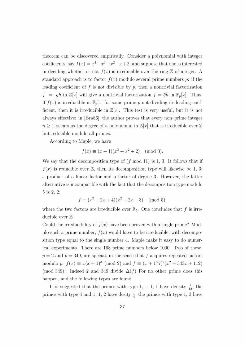
It is suggested that the primes with type 1, 1, 1, 1 have density 112
; the
primes with type 4 and 1, 1, 2 have desity 14; the primes with type 1, 3 have
37
Type 1, 1, 1, 1: 6 primes (4%),
Type 1, 1, 2: 42 primes (25.5%),
Type 2, 2: 21 primes (12.5%),
Type 1, 3: 51 primes (31%),
Type 4: 46 primes (27%).
density 13; finally, to make the densities add up to 1, the primes with type 2, 2
have density 18. Frobenius’s theorem tells how to understand these fractions
through the Galois group of the polynomial.
Let f(x) ∈ Z[x] be a monic polynomial, and denote the degree of f(x) by
n. Assume that the discrimmant ∆(f) does not vanish, so that f(x) has
n distinct zeros α1, α2, · · · , αn in a suitable extension field of the field Q.
Write K for the field generated by these zeros, K = Q(α1, α2, · · · , αn). The
Galois group G of f(x) is the group of field automorphisms of K. Each
σ ∈ G permutes the zeros α1, α2, · · · , αn of f , and is completely determined
by the way in which it permutes these zeros. Hence, we may consider G
as a subgroup of the group Sn of permutations of n symbols. Writing an
element σ ∈ G as a product of disjoint cycles, including cycles of length 1,
and looking at the lengths of these cycles, we obtain the cycle pattern of σ,
which is a partition of n. If p is a prime number not dividing ∆(f), then
we can write f (mod p) as a product of distinct irreducible factors over Fp.
The degrees of these irreducible factors form the decomposition type of f
modulo p; this is also a partition of n. Frobenius’s theorem asserts, roughly
speaking, that the number of prime numbers p with a given decomposition
type is proportional to the number of σ ∈ G with the same cycle pattern. So
we have the following.
Theorem 2.3.1 (Frobenius’s Theorem). The density of the set of prime
p for which f mod p has a given decomposition type n1, n2, · · · , ni, exists, and
it is equal to 1/#Gal(f) times the number of σ ∈ G with decomposition in
disjoint cycle of the form cn1cn2 · · · cni, where cnk
is a nk–cycle.
38
Let us consider the partition in which all ni are equal to 1. Only the
identity permutation has this cycle pattern. Hence the set of primes p for
which f modulo p splits completely into linear factors has density 1/#G.
2.4 Chebotarev’s Theorem
To introduce Chebotarev’s theorem we need the theory of Dedekind’s
Domains explained in Section 1.5.
For any prime ideal p of K unramified in L, the Frobenius element
(p, L/K) = (P, L/K)s.t.P | p
is a conjugacy class in G. Given an element of Gal(L/K), can it be repre-
sented as a Frobenius element of a prime ideal? This question and more is
answered by the following.
Theorem 2.4.1 (Chebotarev’s Density Theorem). Let L be a Galois
extension of number field K, and for σ ∈ Gal(L/K) define Cσ to be the
conjugacy class of σ. Let S be the set of unramified prime ideals p of K such
that for every prime ideal P of L dividing p, the Frobenius element of P is
Cσ. Then S has Dirichlet density
#Cσ
#Gal(L/K).
If S is a set of primes of K, then we define the analytic density of S to
be
δan(S) = limx→∞
#p : #(Ok/p) ≤ x, p ∈ S#p : #(Ok/p) ≤ x, p prime
if this limit exists. If the analytic density exists, then it is actually equal to
the Dirichlet density
δan(S) = lims→1+
(∑p∈S
1
#(OK/p)s
)( ∑p prime
1
#(OK/p)s
)−1
.
The converse is not true: there are cases where the Dirichlet density exists
but the analytic one does not. However, the Chebotarev Density Theorem
is valid with either notion of density.
39
2.5 Frobenius and Chebotarev
In the last section we said that Chebotarev generalized Frobenius’s theo-
rem. In order to explain it clearly, let us consider the following reformulation.
Theorem 2.5.1 (Chebotarev’s Density Theorem). Let f(x) ∈ Z[x] be
a monic polynomial. Assume that the discriminant ∆(f) of f(x) does not
vanish. Let C be a conjugacy class of the Galois group G of f(x). Then the
set of primes p not dividing ∆(f) for which σp belongs to C has a density,
and this density equals |C|/|G|.
On first inspection, one might feel that Chebotarev’s theorem is not much
stronger than Frobenius’s version. In fact, applying the latter to a well–
chosen polynomial, with the same splitting field of f(x), one finds a variant
of the density theorem in which C is required to be a division of G rather
than a conjugacy class; here we say that two elements of G belong to the
same if the cyclic subgroups that they generate are conjugate in G. Frobenius
himself reformulated his theorem already in this way. The partition of G into
divisions is, in general, less fine than its partition into conjugacy classes and
Frobenius’s theorem is correspondingly weaker than Chebotarev’s.
Let σ = (1 2 3 4) be such that the cyclic group is C4 = 〈σ〉. Table 2.1 shows
the difference between these partitions.
Conjugacy classes of C4 id σ σ3 σ2Divisions of C4 id σ, σ3 σ2
Table 2.1: Partition of C4 into divisions and conjugacy classes.
Applying Frobenius’s and Chebotarev’s theorem to the 10–th cyclotomic
polynomial Φ10(x) = x4−x3 +x2−x+1, which has Galois group C4, we get
the distributions shown in Table 2.2.
We computed Table 2.2 just considering primes p ≤ 1000. In particular,
from the second line in Table 2.2 we get the cycle distribution of Gal(f) and
40

C4 id σ σ3 σ2 C4 id σ, σ3 σ2Chebotarev 5
211984
47168
14
Frobenius 40167
89167
38167
Table 2.2: Chebotarev’s and Frobenius’s informations.
from these datas we conclude that Gal(f) ' C4. Increasing the range, the
distributions will be closer to the theoretical results given in Table 2.3.
C4 id σ σ3 σ2 C4 id σ, σ3 σ2Chebotarev 1
414
14
14
Frobenius 14
12
14
Table 2.3: Theoretical informations.
2.6 Dirichlet’s Theorem on Primes in Arith-
metic Progression
Chebotarev’s density theorem may be regarded as the least common gen-
eralization of Dirichlet’s theorem on primes in arithmetic progressions (1837)
and Frobenius’s theorem (1880; published 1896). Dirichlet’s theorem is easy
to discover experimentally. Here are the prime numbers below 100, arranged
by final digit:
1 : 11; 31; 41; 61; 71
2 : 2
3 : 3; 13; 23; 43; 53; 73; 83
5 : 5
7 : 7; 17; 37; 47; 67; 97
9 : 19; 29; 59; 79; 89
41
It does not come as a surprise that no prime numbers end in 0, 4, 6, or 8, and
that only two prime numbers end in 2 or 5. The table suggests that there are
infinitely many primes ending in each of 1, 3, 7, 9, and that, approximately,
they keep up with each other. This is indeed true; it is the special case
m = 10 of the following theorem, proved by Dirichlet in 1837. Write ϕ(m)
for the Euler function evaluated in m. Our goal is to prove the following.
Theorem 2.6.1 (Dirichlet’s Theorem). Let m be a positive integer. Then
for each integer a with gcd(a, m) = 1 the set S of prime numbers p such that
p ≡ a (mod m) has density 1/ϕ(m).
Hence we will show that there are ”equally many” prime numbers p ≡ a
(mod m) for each a ∈ (Z/mZ)∗.
To see how Dirichlet’s theorem follows, let K = Q and let L = Q(ζm), where
ζm is one of the primitive m–th roots of unity. Q(ζm) is an abelian extension
of Q and we can identify its Galois group with (Z/mZ)∗; so Cσ = σ for all
σ ∈ Gal(Q(ζm)/Q), and the Frobenius element of P is just
(p, Q(ζm)/Q) = p (mod m) ∈ (Z/mZ)∗
for all P dividing any prime number p - m, as explained in Example 1.6.8.
Thus we see that there is a bijective correspondence between the conjugacy
classes (mod m) of prime numbers that do not divide m and the elements of
the Galois group, so that the set S in the statement of the theorem becomes
Sa = prime numbers p ∈ Z s.t. p ≡ a (mod m). Since #Cσ = 1 and
#Gal(Q(ζm)/Q) = ϕ(m), the theorem tells us that the set Sa has density
1/ϕ(m) for each a ∈ (Z/mZ)∗, which is exactly Dirichlet’s theorem.
We can follow the same strategy using Frobenius’s theorem, instead of Cheb-
otarev’s. However, this choice does not work for all m.
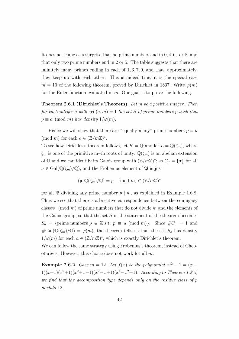
Example 2.6.2. Case m = 12. Let f(x) be the polynomial x12 − 1 = (x −1)(x+1)(x2+1)(x2+x+1)(x2−x+1)(x4−x2+1). According to Theorem 1.2.5,
we find that the decomposition type depends only on the residue class of p
modulo 12.
42
p ≡ 1 (mod 12) ⇒ (1)12
p ≡ 5 (mod 12) ⇒ (1)4, (2)4
p ≡ 7 (mod 12) ⇒ (1)6, (2)3
p ≡ 11 (mod 12) ⇒ (1)2, (2)5
Table 2.4: Decomposition types of f(x) = x12 − 1 modulo different primes.
Looking at Table 2.4 we conclude that Frobenius’s theorem implies Dirich-
let’s theorem in the case m = 12, since the four decomposition type are pair-
wise distinct.
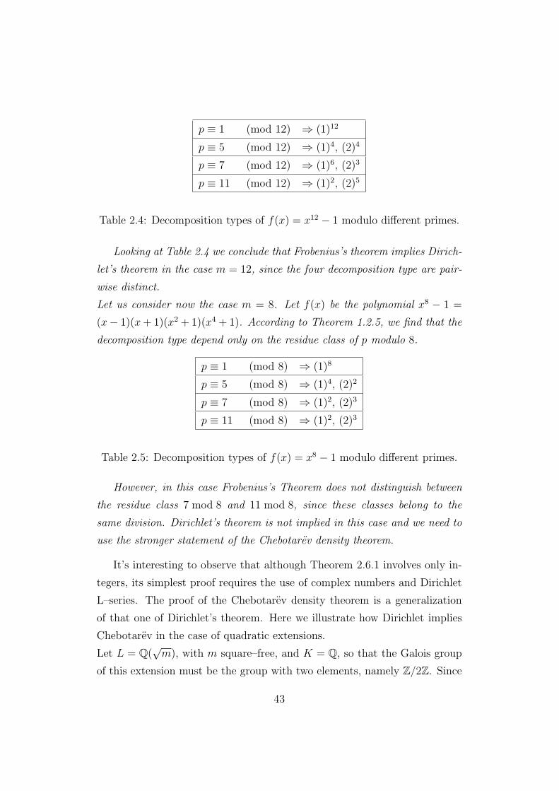
Let us consider now the case m = 8. Let f(x) be the polynomial x8 − 1 =
(x− 1)(x + 1)(x2 + 1)(x4 + 1). According to Theorem 1.2.5, we find that the
decomposition type depend only on the residue class of p modulo 8.
p ≡ 1 (mod 8) ⇒ (1)8
p ≡ 5 (mod 8) ⇒ (1)4, (2)2
p ≡ 7 (mod 8) ⇒ (1)2, (2)3
p ≡ 11 (mod 8) ⇒ (1)2, (2)3
Table 2.5: Decomposition types of f(x) = x8 − 1 modulo different primes.
However, in this case Frobenius’s Theorem does not distinguish between
the residue class 7 mod 8 and 11 mod 8, since these classes belong to the
same division. Dirichlet’s theorem is not implied in this case and we need to
use the stronger statement of the Chebotarev density theorem.
It’s interesting to observe that although Theorem 2.6.1 involves only in-
tegers, its simplest proof requires the use of complex numbers and Dirichlet
L–series. The proof of the Chebotarev density theorem is a generalization
of that one of Dirichlet’s theorem. Here we illustrate how Dirichlet implies
Chebotarev in the case of quadratic extensions.
Let L = Q(√
m), with m square–free, and K = Q, so that the Galois group
of this extension must be the group with two elements, namely Z/2Z. Since
43

this group is abelian, every element has only one conjugate. Thus, viewing
the Galois group as an multiplicative group, the primes with Frobenius ele-
ment 1 must have density 1/2, as should the primes with Frobenius element
−1. Now, from the definition of the Frobenius element, we know that, in
this case, primes that remain prime in OL should correspond to a Frobenius
element of order 2, and primes that split into two primes in OL should cor-
respond to a Frobenius element of order 1; this results from the fact that
the order of the Frobenius element is f = f(P/p), the relative degree of p.
Thus, what Chebotarev’s theorem states in this case is that the density of
the set of primes that split and the density of primes that remain prime in
OL is 1/2. In Example 1.6.11 we have seen that there is a simple way to
characterize each of these sets: p = pZ remains prime in OL if and only if m
is not a square modulo p.
Our statement becomes: the density of primes p such that a given square–
free integer m is a square mod p is 1/2. In the following arguments, we might
be concerned about the case where p | m. We have actually already thrown
out these cases by discarding ramified primes. From Theorem 1.5.9 we know
that such primes are exactly those which divide the discriminant and, in this
case, the discriminant is divisible by m. Now we are ready to use Dirichlet’s
theorem on primes in arithmetic progressions to prove the following.
Proposition 2.6.3. For a quadratic extention Q(√
m), Dirichlet’s theorem
implies Cheboterev’s theorem.
Proof. First, consider(
pq
)where q is an odd prime. If q ≡ 1 mod 4,
(pq
)=(
qp
)for all p. Since half the residues modulo any integer are squares, this
gives us our result in the case where q ≡ 1 mod 4, since exactly ϕ(q)/2
residues are squares modulo q and the density of the set of primes congruent
to each residue is 1/ϕ(q), so the density of primes which are squares modulo
q isϕ(q)
2
1
ϕ(q)=
1
2,
and the primes that are squares modulo q are exactly the primes for which
44
q is a square.
The other case, q ≡ 3 mod 4, is more difficult. If p ≡ 1 mod 4,(
pq
)=(
qp
),
but if p ≡ 3 mod 4,(
qp
)= −
(pq
). To deal with this, consider Dirichlet’s
theorem applied to 4q. This tells us that the density of the primes in each
equivalence class of (Z/(4q)Z)∗ is 1/ϕ(4q). The Chinese remainder theorem
says that exactly half these equivalence classes contain the primes congruent
to 1 mod 4. Thus, if we consider only the set of primes congruent to 1 mod 4,
the primes in this set congruent to a given a ∈ (Z/qZ)∗ must have density
1/ϕ(q). For primes in this set,(
qp
)=(
pq
), so the density of primes in
this set for which q is a square must be 1/2. Considering the set of primes
congruent to 3 mod 4, the fact that the density of primes in this set which
are not squares modulo q must be 1/2 gives us the same result. Thus the
density of all primes for which q is a square must be 1/2.
Now, if we let m = q1q2 · · · qn where all the qi are distinct, we can obtain the
same result if we consider that the primes congruent to 1 mod 4 are equally
distributed over Z/mZ and that for primes p in this set,(q1q2 · · · qn−1
p
)is completely determined by the residue of p mod (q1q2 · · · qn−1). Then if we
consider the subset A of these primes congruent to a given a mod (q1q2 · · · qn−1),
the subset of primes in A congruent to a given b mod (qn) must have density
ϕ(qn) in A. Then (m
p
)=
(q1q2 · · · qn−1
p
)(qn
p
).
For primes in A, the former factor is constant, and the set of primes for which
the latter factor is 1 has density 1/2. Thus m is a square modulo p for half
the primes in A. Since a was arbitrary, the density of primes congruent to
1 mod 4 for which m is a square must be 1/2. A similar argument applies
for the primes congruent to 3 mod 4, so we achieve our result in general: the
density of primes for which a given m is a square is 1/2.
45

2.7 Hint of the Proof
In this section we give a proof of Chebotarev’s theorem that follows his
original strategy, not including class field theory. We refer to [SL96] for more
details.
Let L/K be a finite Galois extension with G = Gal(L/K). For all primes
p not containing the discriminant ideal (∆(L/K)) there exists a Frobenius
element σp, which is an element of G well defined up to conjugacy.
Theorem 2.7.1 (Chebotarev’s theorem). For any conjugacy class C of
G, the density d(L/K, C) of the set S = p ∈K s.t. σp ∈ C exists and equals
#C/#G.
Proof. The first step in our proof is the reduction to the abelian case. Let
σ ∈ C and E = x ∈ L s.t. σx = x. Then L is a Galois extension of E
with Gal(L/E) = 〈σ〉. Chapter 8 of [Lan94] shows that the conclusion of
the theorem holds for L, K, C if and only if it holds for L, E, σ. Note
that Gal(L/E) is abelian, since E = L〈σ〉. Next one considers the case that
L is cyclotomic over K and proves the theorem in this case, as explained
in [SL96].
With this tools we are able to approach a general proof. We assume L/K
to be an abelian extension of degree n, with G = Gal(L/K). Let mOK be
a prime not ramified, and ζ = ζm. Then H = Gal(K(ζ)/K) ' (Z/mZ)∗
and Gal(L(ζ)/K) ' G×H. If a prime p of K has Frobenius element (σ, τ)
in G × H, then it has Frobenius element σ in G. Hence δinf (L/K, σ) ≥∑τ∈H δinf (L(ζ)/K, (σ, τ)). If we fix σ and τ , and suppose that n divides
ordH(τ), then 〈(σ, τ)〉 ∩ G × 1 is the trivial group, and therefore, M =
L〈(σ,τ)〉 satisfies M(ζ) = L(ζ). So L(ζ)/M is a cyclotomic extension. But
we have assumed that in this case the theorem holds, i.e. δL(ζ)/M, (σ, τ)exists and has the correct value; then the same holds for δL(ζ)/K, (σ, τ),which equals 1/(#G·#H). Let Hn = τ ∈ H s.t. n|ordH(τ); then δinf (L/K), σ ≥∑
τ∈H 1/(#G · #H) = #Hn/(#G · #H). When m ranges over all primes
not ramified in L, the fraction #Hn/#H gets arbitrarily close to 1, so that
46

δinf (L/K) ≥ 1/#G. Applying this to all other elements of the group one
finds that δsup(L/K, σ) ≤ 1/#G; hence δ(L/K, σ) = 1/#G.
47

Chapter 3
Applications
3.1 Charming Consequences
First, we have an interesting result about primes p for which (f mod p)
has no zeros. For the following we refer to [Ser03].
Theorem 3.1.1. Let f(x) ∈ Z[x] be an irreducible polynomial of degree
n > 1. If p is prime, let Np(f) be the number of zeros of f in Fp = Z/pZ.
Then there are infinitely many p’s such that Np(f) = 0. Moreover the set
P0(f) of p’s with Np(f) = 0 has a density c0 = c0(f) ≥ 1/n.
To prove the statement above we will use the Burneside Lemma, for which
we refer to [Rot95].
Notation 3.1.2. If ϕ is a function on G, and S ⊂ G, we denote by∫
Sϕ the
number 1|G|∑
g∈S ϕ(g). When S = G, we write∫
ϕ instead of∫
Gϕ.
Lemma 3.1.3 (Burniside’s Lemma). If X is a finite G–set and χ(g) is
the number of fixed points of g on X, then the number of G–orbits of X is
equal to1
|G|∑g∈G
χ(g) =
∫χ.
Proof. In∑
g∈G χ(g), each x ∈ X is counted |StabG(x)| times. If x and y lie in
the same orbit, then |StabG(x)| = |StabG(y)| because they are conjugated in
48
G. So the (G : StabG(x)) elements constituing the orbit of x are collectively
counted (G : StabG(x))|StabG(x)| times. Each orbit thus contributes |G| to
the sum, and so we have 1|G|∑
g∈G χ(g) orbits.
Corollary 3.1.4. If X is a finite transitive G–set with |X| > 1, then there
exists g ∈ G having no fixed points.
Proof. Since the action of G on X is transitive, the number of G–orbits is 1,
and so Burnside’s Lemma gives
1 =1
|G|∑g∈G
χ(g).
Now χ(1) = |X| > 1. If χ(g) ≥ 1 for every g ∈ G, then the right hand side
is too large.
We are ready to prove Theorem 3.1.1.
Proof. Let χ2(g) be the number of points of X ×X fixed by g ∈ G and∫
χ2
be the number of orbits of G on X × X. Then is∫
χ2 ≥ 2, as one sees by
decomposing X ×X into the diagonal and its complement. We will denote
with G0 the set of g ∈ G with χ(g) = 0. If g /∈ G0, we have 1 ≤ χ(g) ≤ n
and therefore
(χ(g)− 1)(χ(g)− n) ≤ 0.
Hence ∫G−G0
(χ(g)− 1)(χ(g)− n) ≤ 0,
that is ∫G
(χ(g)− 1)(χ(g)− n) ≤∫
G0
(χ(g)− 1)(χ(g)− n) ≤ n
∫G0
1.
The left hand side is ∫G
(χ2 − (n + 1)χ + n),
while the right hand side is
n
∫G0
1 = n1
|G|∑g∈G0
1 = n|G0||G|
= nc0.
49
Finally,∫
χ = 1, since the action is transitive. From Lemma 3.1.3 we have∫G
(χ2 − (n + 1)χ + n) ≥ 2− (n + 1) + n = 1,
hence 1 ≤ nc0. To conclude our proof, we use Chebotarev’s Density Theorem.
Let f(x) ∈ Z[x] be the polynomial in the statement and X = α1, . . . , αn be
the set of its distinct roots. We know that G = Gal(f) acts transitively on X.
Now, we denote with G0 the set σ ∈ G with no fixed points; from the above
result, |G0|/|G| ≥ 1/n. The key–observation is that Np(f) = 0 ⇔ σp ∈ G0,
since the decomposition type of (f mod p) equals the cycle pattern of the
Frobenius element σ = σp ∈ G, and so every fixed point of σp corresponds
to a linear factor, i.e. to a root, of (f mod p). Moreover, G0 is stable under
conjugation so that, from Theorem 2.5.1, the set p s.t. σp ∈ G0 has density
c0 = |G0|/|G| ≥ 1n. Thus there are infinitely many p’s such that Np(f) =
0
Note also that Burnside’s Lemma, combined with Chebotarev’s Density
Theorem, gives the following result, due to Kronecker.
Theorem 3.1.5. Let f be as in Theorem 3.1.1. Then the mean value of
Np(f) for p →∞ is equal to 1.
In fact, if G acts transitively on X, then from Lemma 3.1.3 we have
1 =1
|G|∑g∈G
χ(g),
so that the mean value of χ(g) is 1, for each g ∈ G. But each g ∈ G can
be seen as the Frobenius element σp, for some p, whose cycle pattern equals
the decomposition type of (f mod p). Therefore the mean value of zeros of
(f mod p) is 1.
In other words, ∑p≤x
Np(f) ≈ π(x) when x →∞.
It’s very easy to test this formula for any irreducible polynomial f if we know
the cycle type distribution of it’s Galois group.
50

Example 3.1.6. Let f(x) = x3 − 2 so that Gal(f) ' S3. Knowledge of
cycle pattern in Gal(f) allows us to figure out the number of roots modulo
each prime number: they corresponds to the number of fixed point of each
permutation, as explained in Table 3.1.
According to the above result, the mean value of Np(f) is 1. We can prove
this computing ∑(Fixed points) · (Distribution),
where the sum is extended to all cycle type in S3. Hence∑p Np(f)∑
p 1= 3 · 1/6 + 1 · 1/2 = 1
as the theoretical result predicts.
Cycle type (−) (−−) (−−−)
Distribution 16
12
13
Fixed points 3 1 0
Table 3.1: Distribution and fixed points of cycle type in S3.
In Section 2.3 we said that it’s always possible to construct an irreducible
polynomial of non–prime degree which is reducible modulo all primes. What
we can state about polynomial that have a root, that is, a linear factor,
modulo all primes? With a little group theory, we can get our answer to
this question. This result can be found in the article [LS91] by Lenstra and
Stevenhagen.
Theorem 3.1.7. Let f(x) ∈ Z[x] be an irreducible polynomial that has a
zero modulo almost all primes p. Then f(x) is linear.
Proof. Assume that ∂f > 1, and let G be the Galois group of the splitting
field of f . Then G acts transitively on the set Ω of roots of f , and the
assumption that f has a root modulo p for almost all p implies that almost
all Frobenius elements in G fix a root of f . If H ⊂ G is the stabilizer
51
of some ω ∈ Ω, the subset of G consisting of those elements that fix at
least one element of Ω equals⋃
g∈G gHg−1, because we have a transitive
action and StabG(gω) = gStabG(ω)g−1. From Corollary 3.1.4, G contains
at least an element that fix no root of f , and which therefore occurs as
the Frobenius of only finitely many primes in the splitting field of f . This
obviously contradicts the Chebotarev density theorem.
3.2 Primes and Quadratic Forms
For the theory developed in this section we refer to [Cox89]. We will
prove the classical theorem that a primitive positive definite quadratic form
ax2 + bxy + cy2 represents infinitely many prime numbers. We will just
consider particular cases, since a general proof should involve Class Field
Theory.
A first definition is the following.
Definition 3.2.1. A form f(x, y) = ax2 + bxy + cy2 is primitive if a, b, c
are relatively prime.
We will deal exclusively with primitive forms. An integer m is represented
by a form f(x, y) if the equation m = f(x, y) has integer solution in x and
y; if gcd(x, y) = 1, then we say that m is properly represented by f(x, y).
Next, we say that f(x, y) and g(x, y) are equivalent if there are integers
p, q, r, s such that
f(x, y) = g(px + qy, rx + sy) and ps− qr = ±1.
An important observation is that equivalent forms properly represent the
same numbers. Then we say that an equivalence is a proper equivalence if
ps− qr = 1, and it is an improper equivalence if ps− qr = −1.
There is a very nice relation between proper representation and proper equiv-
alence.
Lemma 3.2.2. A form f(x, y) properly represents an integer m if and only
if f(x, y) is properly equivalent to the form mx2+bxy+cy2, for some b, c ∈ Z.
52
Proof. (⇒) suppose that m = f(p, q), with gcd(p, q) = 1. We can find r and
s so that ps− qr = 1, and then
f(px + ry, qx + sy) = f(p, q)x2 + (2apr + bps + brq + 2cqs)xy + f(r, s)y2
= mx2 + bxy + cy2.
(⇐) Note that mx2 + bxy + cy2 represents properly m taking (x, y) = (1, 0).
We define the discriminant of ax2+bxy+cy2 to be D = b2−4ac; equivalent
forms have the same dicriminant. We will consider only positive definite
forms, that is, forms such that a > 0 and D < 0.
We have the following necessary and sufficient condition for a number m to
be represented by a form of discriminant D.
Lemma 3.2.3. Let D ≡ 0, 1 mod 4 be an integer and m be an odd prime
with gcd(D, m) = 1. Then m is properly represented by a primitive form of
discriminant D if and only if(
Dm
)= 1.
Proof. (⇒) From lemma 3.2.2 we may assume f(x, y) = mx2 + bxy + cy2,
since f(x, y) properly represents m. Thus D = b2 − 4mc ≡ b2 mod m.
(⇐) Suppose that D ≡ b2 mod m. Since m is odd, we may assume that
D and b have the same parity, replacing b by b + m if necessary. Then
D ≡ 0, 1 mod 4 implies D ≡ b2 mod 4m. This means that D = b2 − 4mc for
some c. Then mx2+bxy+cy2 represents m properly and has discriminant D,
and the coefficients are relatively prime since m is relatively prime to D.
Corollary 3.2.4. Let n be an integer and let p be an odd prime not dividing
n. Then(−np
)= 1 if and only if p is represented by a primitive form of
discriminant −4n.
Proof. From Lemma 3.2.3, −4n is a quadratic residue modulo p if and only
if(−4n
p
)=(−np
)= 1.
A primitive positive definite form ax2 + bxy + cy2 is said to be reduced if
|b| ≤ a ≤ c, and b ≥ 0 if either |b| = a or a = c.
53
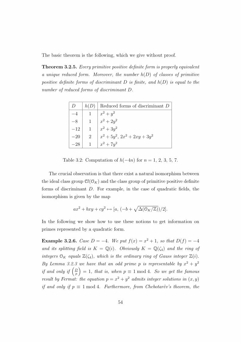
The basic theorem is the following, which we give without proof.
Theorem 3.2.5. Every primitive positive definite form is properly equivalent
a unique reduced form. Moreover, the number h(D) of classes of primitive
positive definite forms of discriminant D is finite, and h(D) is equal to the
number of reduced forms of discriminant D.
D h(D) Reduced forms of discriminant D
−4 1 x2 + y2
−8 1 x2 + 2y2
−12 1 x2 + 3y2
−20 2 x2 + 5y2, 2x2 + 2xy + 3y2
−28 1 x2 + 7y2
Table 3.2: Computation of h(−4n) for n = 1, 2, 3, 5, 7.
The crucial observation is that there exist a natural isomorphism between
the ideal class group Cl(OK) and the class group of primitive positive definite
forms of discriminant D. For example, in the case of quadratic fields, the
isomorphism is given by the map
ax2 + bxy + cy2 7→ [a, (−b +√
∆(OK/Z))/2].
In the following we show how to use these notions to get information on
primes represented by a quadratic form.
Example 3.2.6. Case D = −4. We put f(x) = x2 + 1, so that D(f) = −4
and its splitting field is K = Q(i). Obviously K = Q(ζ4) and the ring of
integers OK equals Z(ζ4), which is the ordinary ring of Gauss integer Z(i).
By Lemma 3.2.3 we have that an odd prime p is representable by x2 + y2
if and only if(
Dp
)= 1, that is, when p ≡ 1 mod 4. So we get the famous
result by Fermat: the equation p = x2 + y2 admits integer solutions in (x, y)
if and only if p ≡ 1 mod 4. Furthermore, from Chebotarev’s theorem, the
54
density of primes such that(
Dp
)= 1 equals 1/2 and therefore we have the
supplementary information
δ(p ≥ 3 s.t. p = x2 + y2) =1
2.
By means of analogous investigations in the case D = −8, −12, −28 we get
δ(p s.t.(−8p
)= 1) = δ(p ≥ 3 s.t. p = x2 + 2y2) = 1
2
δ(p s.t.(−12
p
)= 1) = δ(p ≥ 5 s.t. p = x2 + 3y2) = 1
2
δ(p s.t.(−28
p
)= 1) = δ(p ≥ 11 s.t. p = x2 + 7y2) = 1
2.
The case D = −20 is significantly different and more complicated since
h(−20) > 1 and this fact implies the notion of ring class field. A complete
explaination of this theory leads us to the following general result.
Theorem 3.2.7. Let ax2+bxy+cy2 be a primitive positive definite quadratic
form of discriminant D < 0, and let S be the set of primes represented by
ax2 + bxy + cy2. Then the Dirichlet density δ(S) exists and is given by the
formula
δ(S) =
1
2h(D)if ax2 + bxy + cy2 is properly equivalent to its opposite,
1h(D)
otherwise.
In particular, ax2 + bxy + cy2 represents infinitely many prime numbers.
Therefore, the case D = −20 gives the following result:
δ(p = x2 + 5y2) = δ(p = 2x2 + 2xy + 3y2) =1
2h(D)=
1
4.
3.3 A Probabilistic Approach
The Chebotarev density theorem allows a probabilistic approach to find-
ing G by factoring f modulo different non–ramified primes and cheking for
which transitive subgroups of Sn this approximates the shape distribution
best. Effective bounds on estimates of these distributions have been cal-
culated by Lagarios and Odlyzko in [LO77] using assumptions based on the
55

Generalized Riemann Hypothesis, enabling Gal(f) to be determined uniquely
in many cases.
In the study of Galois groups of polynomial f(x), we restrict ourselves to
monic polynomials with integer coefficients, since any polynomial can easily
be transformed into a monic polynomial with integer coefficients equivalent
with respect to its Galois group, as explained in the following.
Proposition 3.3.1. Let f(x) be a polynomial in Q[x]. Then there exists a
monic polynomial h(x) ∈ Z[x] such that Gal(f) = Gal(h).
Proof. Let f(x) ∈ Q[x]; then f(x) = 1D
g(x), with g(x) ∈ Z[x] and D equal to
a common denominator for the coefficients of f . Let g(x) =∑n
i=0 bixi, bi ∈
Z. Then
g(x) =1
bn−1n
((bnx)n + bn−1(bnx)n−1 + · · ·+ b1b
n−2n (bnx) + b0b
n−1n
)=
1
bn−1n
h(bn(x)),
where h(x) ∈ Z[x] is monic. Hence
h(x) = xn + bn−1xn−1 + · · ·+ b1b
n−2n x + b0b
n−1n = Dbn−1
n f
(x
bn
).
It’s easy to verify that Gal(f) = Gal(h), since Qf = Qh. In fact, if α1, . . . , αn
are n distinct roots of f , i.e. Qf = Q(α1, . . . , αn), then α1bn, . . . , αnbn are n
distinct roots of h, i.e. Qh = Q(α1bn, . . . , αnbn). But bn ∈ Z, so that
Qf = Q(α1, . . . , αn) = Q(α1bn, . . . , αnbn) = Qh.
Thus we need consider only polynomials of the form
f(x) = xn + a1xn−1 + · · ·+ an, ai ∈ Z.
56
Moreover we want f(x) to be irreducible; this restiction is not essential, but
it greatly simplifies the work of implementing the algorithm for polynomials
of a given degree. By the way, let f(x) ∈ Z[x] be a monic polynomial and
f(x) = g(x) · h(x) be its decomposition into irreducible factors, Qg and Qh
being the respective splitting fields. If Qg ∩ Qh = Q, then the Galois group
of f(x) is the direct product Gal(g)×Gal(h). Otherwise, if Qg ∩Qh is larger
than Q, then Gal(f) is not easily determined from those of g(x) and h(x),
without explicit knowledge of the relations between the roots of g and h. In
fact, generally we have
Gal(g · h) = (σi, σj) ∈ Gal(g)×Gal(h) s.t. σi|Qg∩Qh= σj|Qg∩Qh
.
With this assumptions, the strategy for determining the Galois group of
a polynomial f ∈ Z[x] is:
1. test whether f is irreducible over Z;
2. compute the discriminant ∆(f);
3. factor f modulo primes not dividing the discriminant until you seem
to be getting no new decomposition type;
4. compute the orbit lengths on the r–sets of roots;
5. use tables of transitive groups of degree ∂f .
The second point is very useful. In fact, knowledge of ∆(f) allows us to
establish if Gal(f) ⊆ An.
Proposition 3.3.2. Let An be the alternating group on n letters. Then
Gal(f) ⊂ An if and only if ∆(f) is a square.
Proof. Let αi be the roots of f . We know that D(f) = ∆(f)2, where ∆(f) =∏1≤i<j≤n(αi−αj). Clearly ∆(f) is an algebraic integer, since it’s a symmetric
polynomial on α1, . . . , αn. We have σ(∆(f)) = ε(σ)∆(f) ∀σ ∈ Gal(f), where
ε(σ) is the signature of σ. Hence, if Gal(f) ⊂ An, then ∆(f) is invariant
57
under Gal(f), and so ∆(f) ∈ Z. On the other hand, if ∆(f) ∈ Z, we have
∆(f) 6= 0 since the root of an irreducible polynomial in Z[x] are distinct.
Therefore σ(∆(f)) = ∆(f), that is ε(σ) = 1, ∀σ ∈ G, and Gal(f) ⊂ An.
Remark 3.3.3. Consider a permutation σ ∈ Sn,
σ =
(1 2 3 · · · n
σ(1) σ(2) σ(3) · · · σ(n)
)and define η(σ) = (i, j) with i < j and σ(i) > σ(j). Then σ is said to
be even or odd according as the number η(σ) is even or odd. The signature,
ε(σ), of σ is +1 or −1 according as σ is even or odd, i.e., ε(σ) = (−1)η(σ).
With this definition of signature, it’s easily seen that σ(∆(f)) = ε(σ)∆(f),
as we stated above.
The third point is difficult to execute from a computational point of
view: this is a rather expensive technique since algorithms of factorizing
polynomials are not very efficient. Furthermore, many primes p might be
needed in the process. For more detail on the problem, see [LO77].
The fourth point gives an upper bounds for Gal(f) using a method based
on the following lemma. We refer to [EFM79] and [McK79].
Lemma 3.3.4. Let Kα = Q(α1, . . . , αn) and Kβ = Q(β1, . . . , βm), where
βk is the set of the partial sums r at a time, with 0 < r < n, of the αiand m = #βk =
(nr
). Then Kα = Kβ.
Proof. Let r > 1. For every i, j we have αi − αj ∈ Kβ, since αi − αj is the
difference of two of the b’s differing in one place. Suppose that βk =∑
j∈I αj,
where #I = r; then
βk +∑j∈I
(αi − αj) = rαi ∈ Kβ.
If we denote with Pα =∏
(x−αi) and with Pβ =∏
(x−βk), Lemma 3.3.4
yields Gal(Pα) = Gal(Pβ). It’s fundamental to notice that the degrees of the
58

irreducible factors in Q[x] of the polynomial Pβ, whose roots are the sums
of r roots of Pα, equal the orbit lengths on the r–sets of roots. In particular
the following holds.
Proposition 3.3.5. Let Pβ be the above polynomial and assume that it has
only distinct zeros. Then Pβ is reducible if and only if Gal(Pα) is not r–
transitive on αi.
If we can prove by the Chebotarev density theorem that
G ⊆ Gal(f) ⊆ An,
where G is maximal in An, then Proposition 3.3.5 will usually determine
Gal(f). In [McK79], the author describes and uses this method to find poly-
nomials with Galois group PSL3(F2) and M11: the first one is a maximal
subgroup of the alternating group A7, while the second one is the Mathieu
group of degree 11, which is a maximal subgroup of A11. Here below, we
illustrate how this test works.
Example 3.3.6. Let Pα(x) = x5−5x+12 and A be the set of its roots, which
we denote with α1, . . . , α5. If r = 2, then B = α1 + α2, α1 + α3, α1 +
α4, α1+α5, α2+α3, α2+α4, α2+α5, α3+α4, α3+α5, α4+α5. Suppose, after
several mod p reductions, that we have two possibilities for G = Gal(Pα), i.e.
D5 ⊆ G ⊆ A5. Computing Pβ(x) =∏
βi∈B(x− βi), we get
Pβ(x) = (x5 − 5x3 − 10x2 − 30x− 36)(x5 + 5x3 + 10x2 + 10x + 4).
Therefore Gal(Pα) is not 2–transitive. This information gives us the desired
upper bound: in fact, since An is (n − 2)–transitive, the only possibility is
Gal(Pα) = D5.
Remark 3.3.7. Proposition 3.3.5 gives information on r–fold transitivity,
i.e. transitivity on r–sets, rather than on r–transitivity. However these two
concepts are the same in many cases. In particular, for r = 2 we have that
a group G is 2–transitive if and only if G is 2–fold transitive, and therefore
the result in Example 3.3.6 is correct.
59
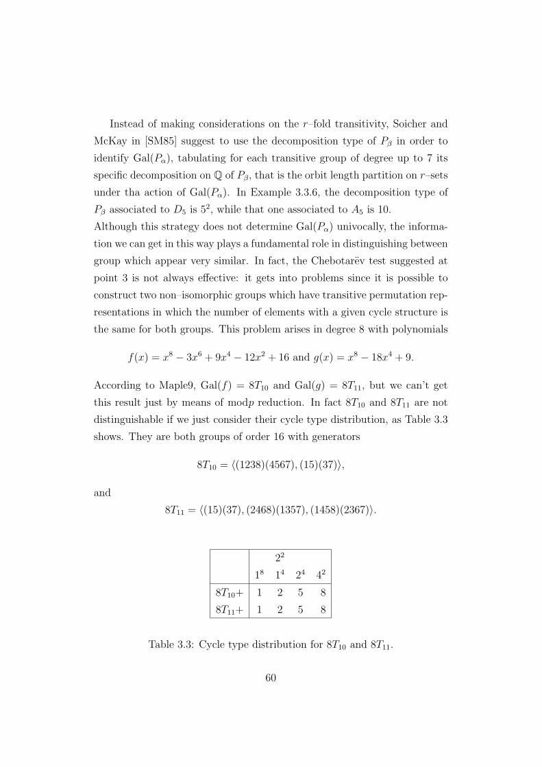
Instead of making considerations on the r–fold transitivity, Soicher and
McKay in [SM85] suggest to use the decomposition type of Pβ in order to
identify Gal(Pα), tabulating for each transitive group of degree up to 7 its
specific decomposition on Q of Pβ, that is the orbit length partition on r–sets
under tha action of Gal(Pα). In Example 3.3.6, the decomposition type of
Pβ associated to D5 is 52, while that one associated to A5 is 10.
Although this strategy does not determine Gal(Pα) univocally, the informa-
tion we can get in this way plays a fundamental role in distinguishing between
group which appear very similar. In fact, the Chebotarev test suggested at
point 3 is not always effective: it gets into problems since it is possible to
construct two non–isomorphic groups which have transitive permutation rep-
resentations in which the number of elements with a given cycle structure is
the same for both groups. This problem arises in degree 8 with polynomials
f(x) = x8 − 3x6 + 9x4 − 12x2 + 16 and g(x) = x8 − 18x4 + 9.
According to Maple9, Gal(f) = 8T10 and Gal(g) = 8T11, but we can’t get
this result just by means of modp reduction. In fact 8T10 and 8T11 are not
distinguishable if we just consider their cycle type distribution, as Table 3.3
shows. They are both groups of order 16 with generators
8T10 = 〈(1238)(4567), (15)(37)〉,
and
8T11 = 〈(15)(37), (2468)(1357), (1458)(2367)〉.
22
18 14 24 42
8T10+ 1 2 5 8
8T11+ 1 2 5 8
Table 3.3: Cycle type distribution for 8T10 and 8T11.
60
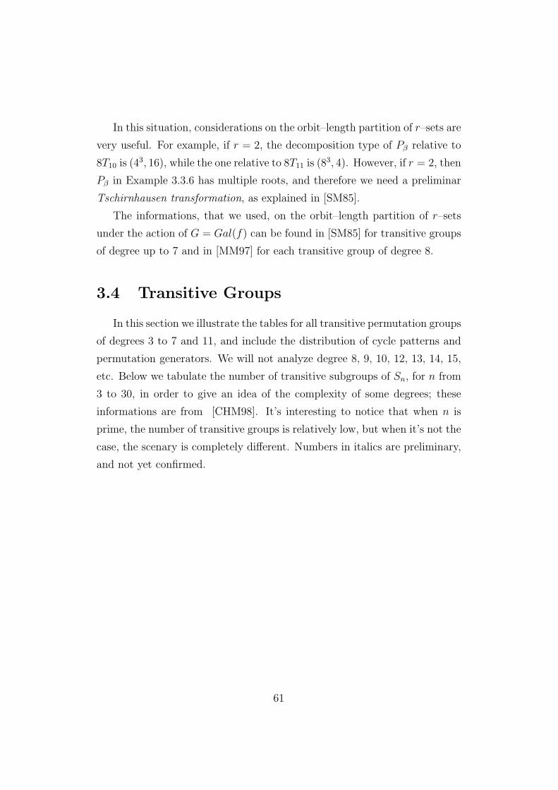
In this situation, considerations on the orbit–length partition of r–sets are
very useful. For example, if r = 2, the decomposition type of Pβ relative to
8T10 is (43, 16), while the one relative to 8T11 is (83, 4). However, if r = 2, then
Pβ in Example 3.3.6 has multiple roots, and therefore we need a preliminar
Tschirnhausen transformation, as explained in [SM85].
The informations, that we used, on the orbit–length partition of r–sets
under the action of G = Gal(f) can be found in [SM85] for transitive groups
of degree up to 7 and in [MM97] for each transitive group of degree 8.
3.4 Transitive Groups
In this section we illustrate the tables for all transitive permutation groups
of degrees 3 to 7 and 11, and include the distribution of cycle patterns and
permutation generators. We will not analyze degree 8, 9, 10, 12, 13, 14, 15,
etc. Below we tabulate the number of transitive subgroups of Sn, for n from
3 to 30, in order to give an idea of the complexity of some degrees; these
informations are from [CHM98]. It’s interesting to notice that when n is
prime, the number of transitive groups is relatively low, but when it’s not the
case, the scenary is completely different. Numbers in italics are preliminary,
and not yet confirmed.
61
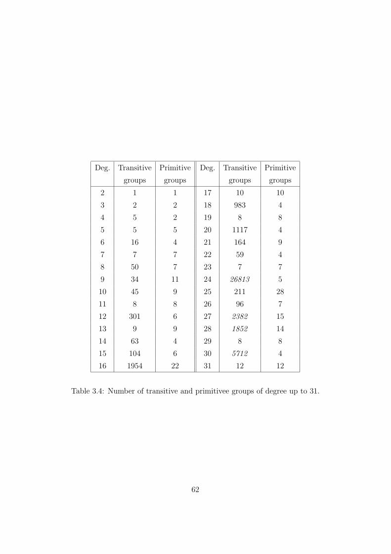
Deg. Transitive Primitive Deg. Transitive Primitive
groups groups groups groups
2 1 1 17 10 10
3 2 2 18 983 4
4 5 2 19 8 8
5 5 5 20 1117 4
6 16 4 21 164 9
7 7 7 22 59 4
8 50 7 23 7 7
9 34 11 24 26813 5
10 45 9 25 211 28
11 8 8 26 96 7
12 301 6 27 2382 15
13 9 9 28 1852 14
14 63 4 29 8 8
15 104 6 30 5712 4
16 1954 22 31 12 12
Table 3.4: Number of transitive and primitivee groups of degree up to 31.
62
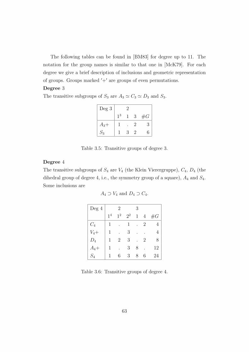
The following tables can be found in [BM83] for degree up to 11. The
notation for the group names is similar to that one in [McK79]. For each
degree we give a brief description of inclusions and geometric representation
of groups. Groups marked ′+′ are groups of even permutations.
Degree 3
The transitive subgroups of S3 are A3 ' C3 ' D3 and S3.
Deg 3 2
13 1 3 #G
A3+ 1 . 2 3
S3 1 3 2 6
Table 3.5: Transitive groups of degree 3.
Degree 4
The transitive subgroups of S4 are V4 (the Klein Vierergruppe), C4, D4 (the
dihedral group of degree 4, i.e., the symmetry group of a square), A4 and S4.
Some inclusions are
A4 ⊃ V4 and D4 ⊃ C4.
Deg 4 2 3
14 12 22 1 4 #G
C4 1 . 1 . 2 4
V4+ 1 . 3 . . 4
D4 1 2 3 . 2 8
A4+ 1 . 3 8 . 12
S4 1 6 3 8 6 24
Table 3.6: Transitive groups of degree 4.
63

Degree 5
The transitive subgroups of S5 are C5, D5 (the dihedral group of degree 5,
i.e., the symmetries of a regular pentagon), F20 (the Frobenius group of order
20, i.e., the affine maps on F5), A5 and S5. The inclusions are
A5 ⊃ D5 ⊃ C5 and F20 ⊃ D5,
meaning that C5, D5 and A5 correspond to square discriminant, and F20
and S5 to non–square discriminant. The groups C5, D5 and F20 are solvable
groups, while A5 is simple.
Deg 5 2 22 3 3 4
15 13 1 2 12 1 5 #G
C5+ 1 . . . . . 4 5
D5+ 1 . 5 . . . 4 10
F20 1 . 5 . . 10 4 20
A5+ 1 . 15 . 20 . 24 60
S5 1 10 15 20 20 30 24 120
Table 3.7: Transitive groups of degree 5.
64
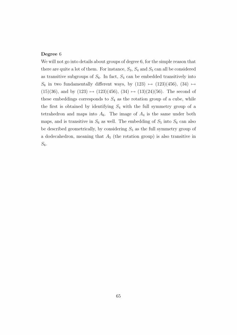
Degree 6
We will not go into details about groups of degree 6, for the simple reason that
there are quite a lot of them. For instance, S3, S4 and S5 can all be considered
as transitive subgroups of S6. In fact, S4 can be embedded transitively into
S6 in two fundamentally different ways, by (123) 7→ (123)(456), (34) 7→(15)(36), and by (123) 7→ (123)(456), (34) 7→ (13)(24)(56). The second of
these embeddings corresponds to S4 as the rotation group of a cube, while
the first is obtained by identifying S4 with the full symmetry group of a
tetrahedron and maps into A6. The image of A4 is the same under both
maps, and is transitive in S6 as well. The embedding of S5 into S6 can also
be described geometrically, by considering S5 as the full symmetry group of
a dodecahedron, meaning that A5 (the rotation group) is also transitive in
S6.
65
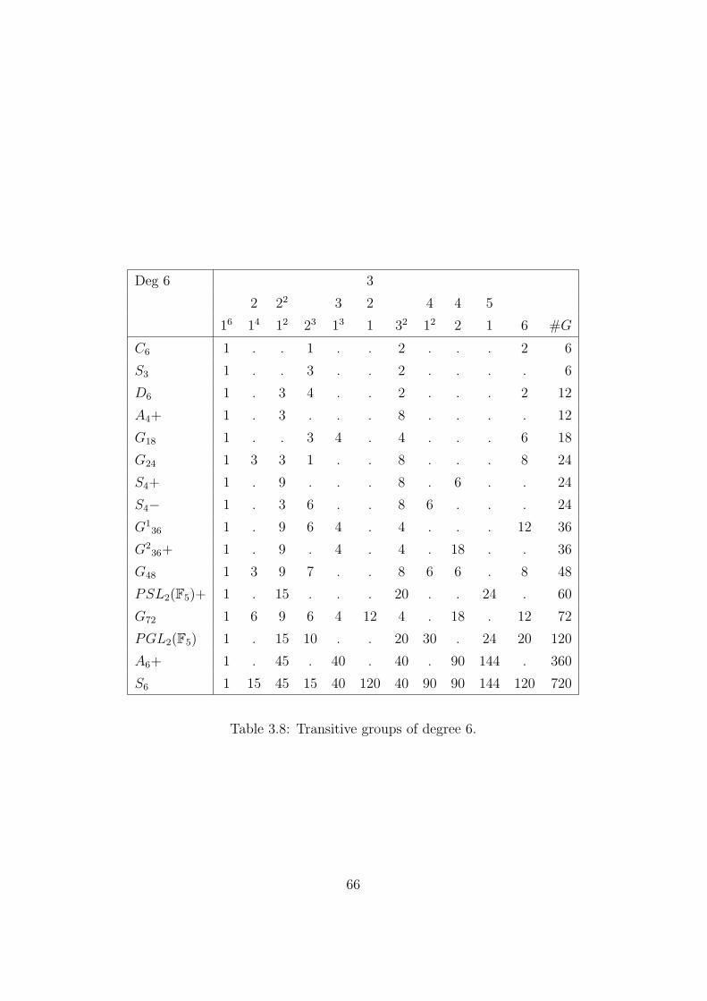
Deg 6 3
2 22 3 2 4 4 5
16 14 12 23 13 1 32 12 2 1 6 #G
C6 1 . . 1 . . 2 . . . 2 6
S3 1 . . 3 . . 2 . . . . 6
D6 1 . 3 4 . . 2 . . . 2 12
A4+ 1 . 3 . . . 8 . . . . 12
G18 1 . . 3 4 . 4 . . . 6 18
G24 1 3 3 1 . . 8 . . . 8 24
S4+ 1 . 9 . . . 8 . 6 . . 24
S4− 1 . 3 6 . . 8 6 . . . 24
G136 1 . 9 6 4 . 4 . . . 12 36
G236+ 1 . 9 . 4 . 4 . 18 . . 36
G48 1 3 9 7 . . 8 6 6 . 8 48
PSL2(F5)+ 1 . 15 . . . 20 . . 24 . 60
G72 1 6 9 6 4 12 4 . 18 . 12 72
PGL2(F5) 1 . 15 10 . . 20 30 . 24 20 120
A6+ 1 . 45 . 40 . 40 . 90 144 . 360
S6 1 15 45 15 40 120 40 90 90 144 120 720
Table 3.8: Transitive groups of degree 6.
66
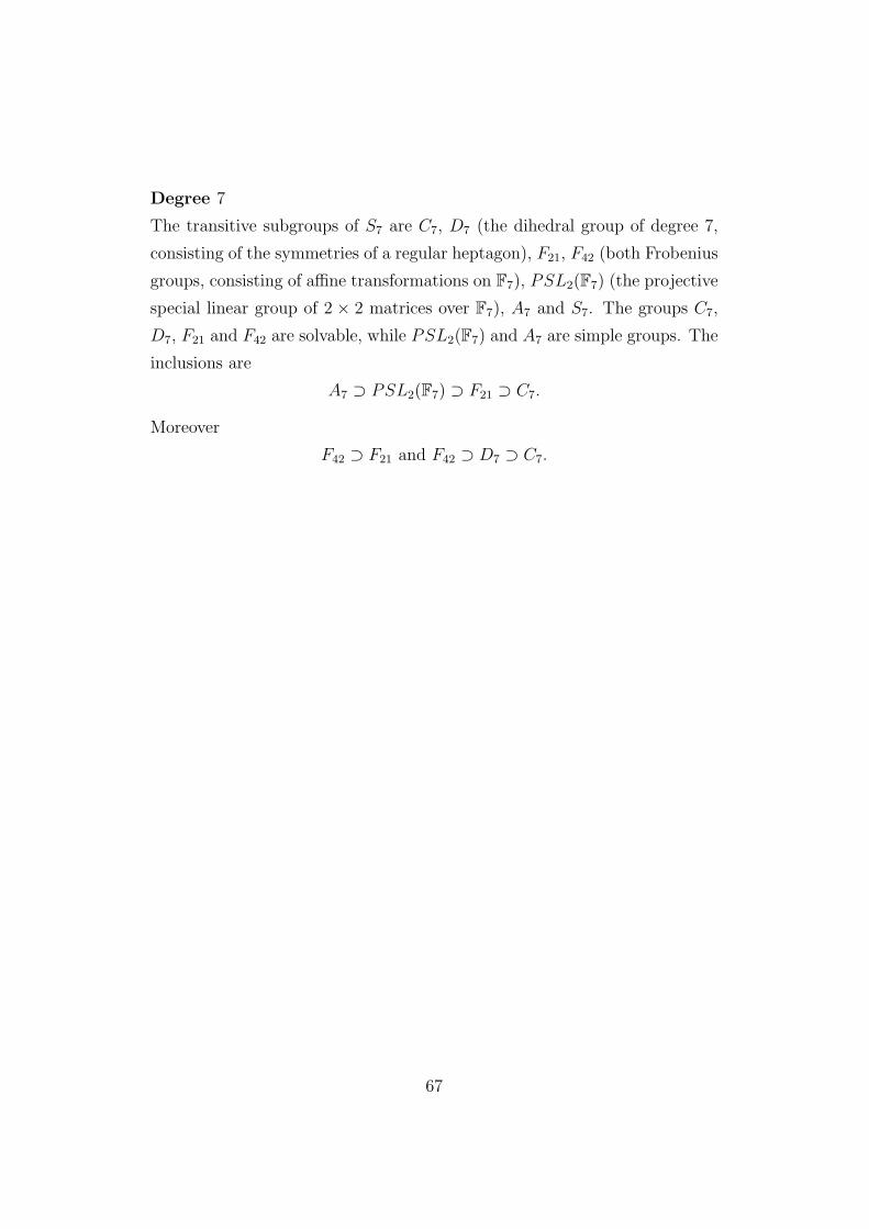
Degree 7
The transitive subgroups of S7 are C7, D7 (the dihedral group of degree 7,
consisting of the symmetries of a regular heptagon), F21, F42 (both Frobenius
groups, consisting of affine transformations on F7), PSL2(F7) (the projective
special linear group of 2 × 2 matrices over F7), A7 and S7. The groups C7,
D7, F21 and F42 are solvable, while PSL2(F7) and A7 are simple groups. The
inclusions are
A7 ⊃ PSL2(F7) ⊃ F21 ⊃ C7.
Moreover
F42 ⊃ F21 and F42 ⊃ D7 ⊃ C7.
67
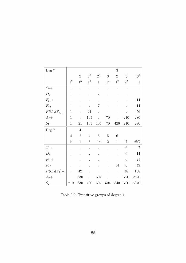
Deg 7 3
2 22 23 3 2 3 32
17 15 13 1 14 12 22 1
C7+ 1 . . . . . . .
D7 1 . . 7 . . . .
F21+ 1 . . . . . . 14
F42 1 . . 7 . . . 14
PSL2(F7)+ 1 . 21 . . . . 56
A7+ 1 . 105 . 70 . 210 280
S7 1 21 105 105 70 420 210 280
Deg 7 4
4 2 4 5 5 6
13 1 3 12 2 1 7 #G
C7+ . . . . . . 6 7
D7 . . . . . . 6 14
F21+ . . . . . . 6 21
F42 . . . . . 14 6 42
PSL2(F7)+ . 42 . . . . 48 168
A7+ . 630 . 504 . . 720 2520
S7 210 630 420 504 504 840 720 5040
Table 3.9: Transitive groups of degree 7.
68

Degree 11
The transitive subgroups of S11 are C11, D11 (the dihedral group), F55, F110
(both Frobenius groups), PSL2(F11) (the projective special linear group),
M11 (the Mathieu group), A11 and S11. The inclusions are
A11 ⊃ M11 ⊃ PSL2(F11) ⊃ F55 ⊃ C11.
Then
F110 ⊃ F55 and F110 ⊃ D11 ⊃ C11.
Since there are 56 different partitions of 11, we don’t give the cycle type of
elements that belongs to An and Sn. However we remember that an element
of cycle type 1a1 , 2a2 , . . . , kak occurs n!/∏k
i=1 iai(ai!) in Sn.
69

Deg 11
24 25 33 42
111 13 1 12 13 #G
C11+ 1 . . . . 11
D11 1 . 11 . . 22
F55+ 1 . . . . 55
F110 1 . 11 . . 110
PSL2(F11)+ 1 55 . 110 . 660
M11+ 1 165 . 440 990 7920
Deg 11 6 8
52 3 2 10
1 2 1 1 11 #G
C11+ . . . . 10 11
D11 . . . . 10 22
F55+ 44 . . . 10 55
F110 44 . . 44 10 110
PSL2(F11)+ 264 110 . . 120 660
M11+ 1584 1320 1980 . 1440 7920
Table 3.10: Transitive groups of degree 11.
70
Chapter 4
Inverse Galois Problem
4.1 Computing Galois Groups
Can any permutation group appear as the Galois group of a polynomial
over the rationals? The answer is positive just for solvable groups and is due
to Shafarevich, as explained in [Saf54]. Shafarevich’s argument, however, is
not constructive and so does not produce a polynomial having a prescribed
finite solvable group as a Galois group. For unsolvable groups, the question
is an open problem. For example, let us consider the the Mathieu group M23.
It is a finite simlpe group of order 27 · 32 · 5 · 7 · 11 · 23 and can be regarded
as a transitive subgroup of S23. However, it’s not known if there exists a
polynomial f(x) ∈ Q[x] such that Gal(f) is the M23, as explained in [Vol96].
In the following tables, partially taken from [SM85], each transitive per-
mutation group of degree from 3 to 7 and 11 is realised as a Galois group
over the rationals. The proof of exactness of these results is verified by the
galois( ) routine implemented in Maple9, which computes the exact Galois
group of polynomials of degree up to 9. For polynomials of degree 11, we use
the polgalois( ) routine implemented in GP/Pari, version 2.3.2, which can
handle polynomial of degree up to 11.
71
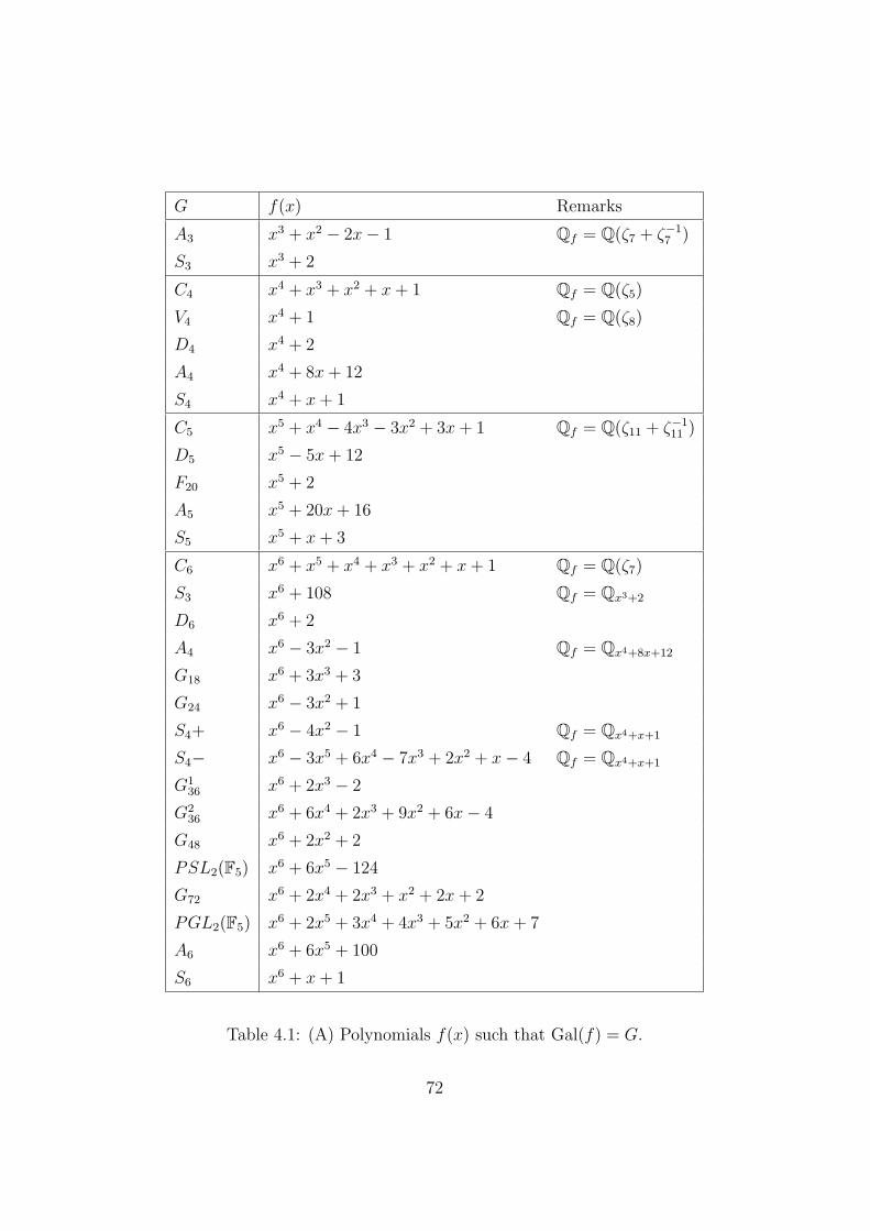
G f(x) Remarks
A3 x3 + x2 − 2x− 1 Qf = Q(ζ7 + ζ−17 )
S3 x3 + 2
C4 x4 + x3 + x2 + x + 1 Qf = Q(ζ5)
V4 x4 + 1 Qf = Q(ζ8)
D4 x4 + 2
A4 x4 + 8x + 12
S4 x4 + x + 1
C5 x5 + x4 − 4x3 − 3x2 + 3x + 1 Qf = Q(ζ11 + ζ−111 )
D5 x5 − 5x + 12
F20 x5 + 2
A5 x5 + 20x + 16
S5 x5 + x + 3
C6 x6 + x5 + x4 + x3 + x2 + x + 1 Qf = Q(ζ7)
S3 x6 + 108 Qf = Qx3+2
D6 x6 + 2
A4 x6 − 3x2 − 1 Qf = Qx4+8x+12
G18 x6 + 3x3 + 3
G24 x6 − 3x2 + 1
S4+ x6 − 4x2 − 1 Qf = Qx4+x+1
S4− x6 − 3x5 + 6x4 − 7x3 + 2x2 + x− 4 Qf = Qx4+x+1
G136 x6 + 2x3 − 2
G236 x6 + 6x4 + 2x3 + 9x2 + 6x− 4
G48 x6 + 2x2 + 2
PSL2(F5) x6 + 6x5 − 124
G72 x6 + 2x4 + 2x3 + x2 + 2x + 2
PGL2(F5) x6 + 2x5 + 3x4 + 4x3 + 5x2 + 6x + 7
A6 x6 + 6x5 + 100
S6 x6 + x + 1
Table 4.1: (A) Polynomials f(x) such that Gal(f) = G.
72
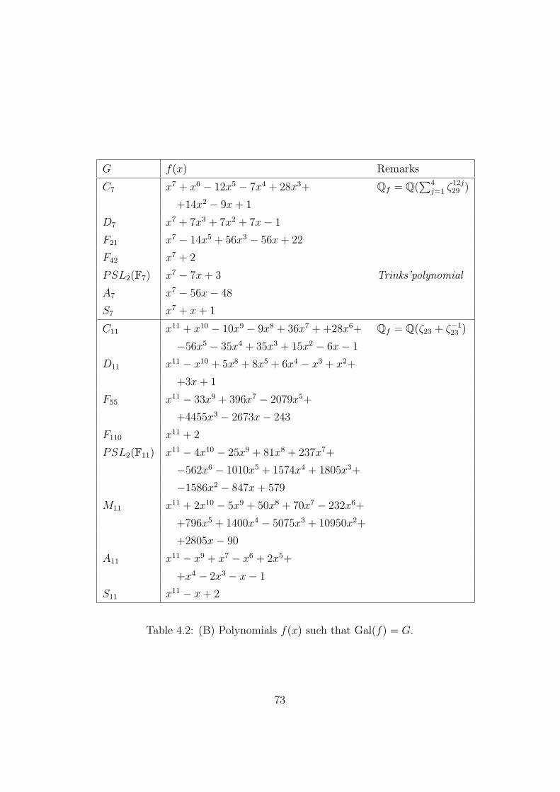
G f(x) Remarks
C7 x7 + x6 − 12x5 − 7x4 + 28x3+ Qf = Q(∑4
j=1 ζ12j29 )
+14x2 − 9x + 1
D7 x7 + 7x3 + 7x2 + 7x− 1
F21 x7 − 14x5 + 56x3 − 56x + 22
F42 x7 + 2
PSL2(F7) x7 − 7x + 3 Trinks’polynomial
A7 x7 − 56x− 48
S7 x7 + x + 1
C11 x11 + x10 − 10x9 − 9x8 + 36x7 + +28x6+ Qf = Q(ζ23 + ζ−123 )
−56x5 − 35x4 + 35x3 + 15x2 − 6x− 1
D11 x11 − x10 + 5x8 + 8x5 + 6x4 − x3 + x2+
+3x + 1
F55 x11 − 33x9 + 396x7 − 2079x5+
+4455x3 − 2673x− 243
F110 x11 + 2
PSL2(F11) x11 − 4x10 − 25x9 + 81x8 + 237x7+
−562x6 − 1010x5 + 1574x4 + 1805x3+
−1586x2 − 847x + 579
M11 x11 + 2x10 − 5x9 + 50x8 + 70x7 − 232x6+
+796x5 + 1400x4 − 5075x3 + 10950x2+
+2805x− 90
A11 x11 − x9 + x7 − x6 + 2x5+
+x4 − 2x3 − x− 1
S11 x11 − x + 2
Table 4.2: (B) Polynomials f(x) such that Gal(f) = G.
73

In Appendix C we write down a Maple code which computes Galois groups
of polynomials using the strategy suggested by the Chebotarev theorem. We
introduce the following definitions in order to describe the code step by step.
Definition 4.1.1. Let n be a positive integer. We define S(n) to be the
ordered set of all the cycle type in the symmetric group Sn, where the order
is the lexicographic one. The cardinality of this set equals the number of
different partitions of n, which we will denote with π(n).
Example 4.1.2. There are 5 different partitions of n = 4. Therefore the
ordered set S(4) equals
(14); (12, 2); (22); (12, 3); (4).
Definition 4.1.3. Let G be a transitive group of degree n. We define the
distribution–vector S(G) to be the vector, with π(n) components, whose j–
th component represents the distribution, in G, of the j–cycle type of S(n).
Namely
S(G)[i] :=|σ ∈ G s.t. σ has cycle type S(n)[i]|
|G|.
Given an irreducible polynomial f(x) ∈ Z[x] of degree n, we can con-
struct a similar distribution–vector S(f) in the following way. Fix a bound
k and consider the primes p ≤ k. For each prime not dividing ∆(f), store
the decomposition type of (f mod p). When each prime in the bound has
been parsed, compute the frequency of each decomposition type. Now, each
decomposition type can be regarded as a partition of n in which the num-
bers that make up the partition are the degrees of the irreducible factors of
(f mod p). Finally complete the empirical distribution–vector S(f) with the
frequency found in this way keeping the lexicographic order, so that
S(f)[i] :=|p ≤ k s.t. p - ∆(f) and (f mod p) has a cycle decomposition of the type S(n)[i]|
|p ≤ k s.t. p - ∆(f)|.
Definition 4.1.4. Let G be a transitive group of degree n and f(x) ∈ Z[x]
be an irreducible polynomial of degree n. We define the error–vector E(G) to
74
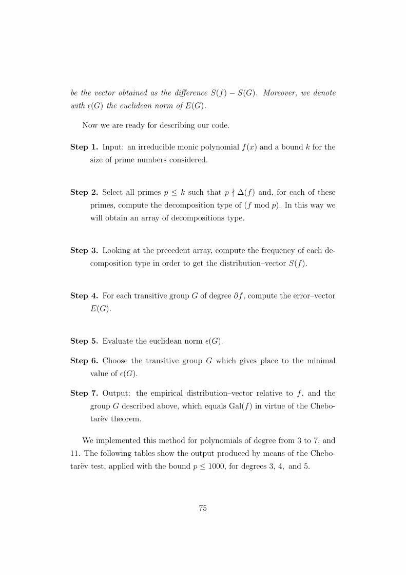
be the vector obtained as the difference S(f) − S(G). Moreover, we denote
with ε(G) the euclidean norm of E(G).
Now we are ready for describing our code.
Step 1. Input: an irreducible monic polynomial f(x) and a bound k for the
size of prime numbers considered.
Step 2. Select all primes p ≤ k such that p - ∆(f) and, for each of these
primes, compute the decomposition type of (f mod p). In this way we
will obtain an array of decompositions type.
Step 3. Looking at the precedent array, compute the frequency of each de-
composition type in order to get the distribution–vector S(f).
Step 4. For each transitive group G of degree ∂f , compute the error–vector
E(G).
Step 5. Evaluate the euclidean norm ε(G).
Step 6. Choose the transitive group G which gives place to the minimal
value of ε(G).
Step 7. Output: the empirical distribution–vector relative to f , and the
group G described above, which equals Gal(f) in virtue of the Chebo-
tarev theorem.
We implemented this method for polynomials of degree from 3 to 7, and
11. The following tables show the output produced by means of the Chebo-
tarev test, applied with the bound p ≤ 1000, for degrees 3, 4, and 5.
75
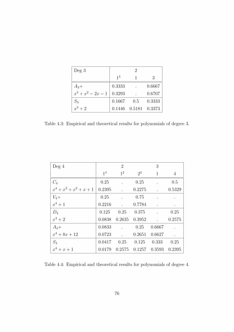
Deg 3 2
13 1 3
A3+ 0.3333 . 0.6667
x3 + x2 − 2x− 1 0.3293 . 0.6707
S3 0.1667 0.5 0.3333
x3 + 2 0.1446 0.5181 0.3373
Table 4.3: Empirical and theoretical results for polynomials of degree 3.
Deg 4 2 3
14 12 22 1 4
C4 0.25 . 0.25 . 0.5
x4 + x3 + x2 + x + 1 0.2395 . 0.2275 . 0.5329
V4+ 0.25 . 0.75 . .
x4 + 1 0.2216 . 0.7784 . .
D4 0.125 0.25 0.375 . 0.25
x4 + 2 0.0838 0.2635 0.3952 . 0.2575
A4+ 0.0833 . 0.25 0.6667 .
x4 + 8x + 12 0.0723 . 0.2651 0.6627 .
S4 0.0417 0.25 0.125 0.333 0.25
x4 + x + 1 0.0179 0.2575 0.1257 0.3593 0.2395
Table 4.4: Empirical and theoretical results for polynomials of degree 4.
76
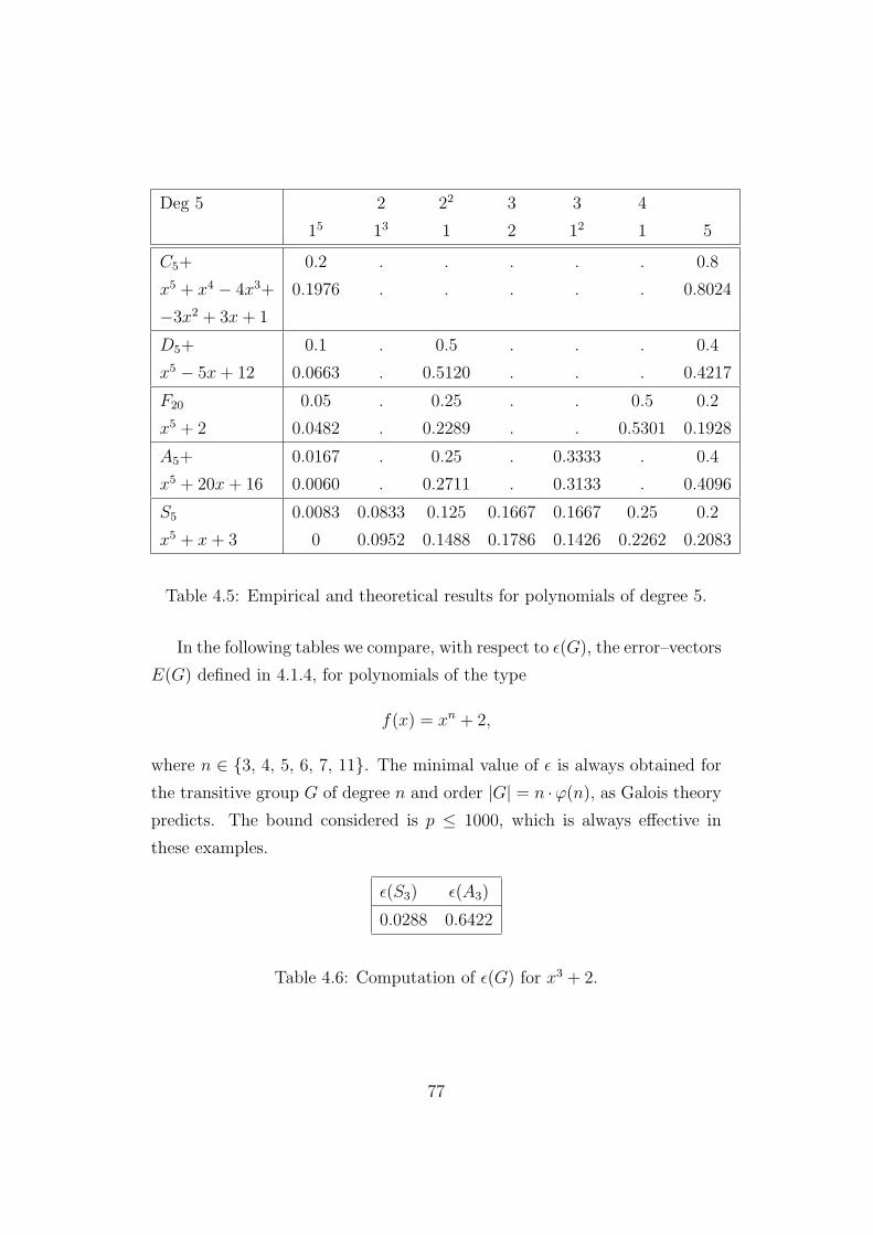
Deg 5 2 22 3 3 4
15 13 1 2 12 1 5
C5+ 0.2 . . . . . 0.8
x5 + x4 − 4x3+ 0.1976 . . . . . 0.8024
−3x2 + 3x + 1
D5+ 0.1 . 0.5 . . . 0.4
x5 − 5x + 12 0.0663 . 0.5120 . . . 0.4217
F20 0.05 . 0.25 . . 0.5 0.2
x5 + 2 0.0482 . 0.2289 . . 0.5301 0.1928
A5+ 0.0167 . 0.25 . 0.3333 . 0.4
x5 + 20x + 16 0.0060 . 0.2711 . 0.3133 . 0.4096
S5 0.0083 0.0833 0.125 0.1667 0.1667 0.25 0.2
x5 + x + 3 0 0.0952 0.1488 0.1786 0.1426 0.2262 0.2083
Table 4.5: Empirical and theoretical results for polynomials of degree 5.
In the following tables we compare, with respect to ε(G), the error–vectors
E(G) defined in 4.1.4, for polynomials of the type
f(x) = xn + 2,
where n ∈ 3, 4, 5, 6, 7, 11. The minimal value of ε is always obtained for
the transitive group G of degree n and order |G| = n ·ϕ(n), as Galois theory
predicts. The bound considered is p ≤ 1000, which is always effective in
these examples.
ε(S3) ε(A3)
0.0288 0.6422
Table 4.6: Computation of ε(G) for x3 + 2.
77
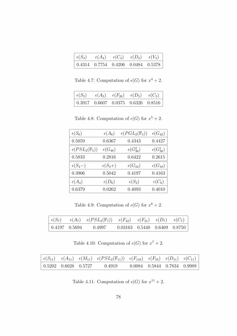
ε(S4) ε(A4) ε(C4) ε(D4) ε(V4)
0.4314 0.7754 0.4206 0.0484 0.5378
Table 4.7: Computation of ε(G) for x4 + 2.
ε(S5) ε(A5) ε(F20) ε(D5) ε(C5)
0.3917 0.6607 0.0375 0.6326 0.8516
Table 4.8: Computation of ε(G) for x5 + 2.
ε(S6) ε(A6) ε(PGL2(F5)) ε(G42)
0.5059 0.6367 0.4343 0.4427
ε(PSL2(F5)) ε(G48) ε(G236) ε(G1
36)
0.5833 0.2816 0.6422 0.2615
ε(S4−) ε(S4+) ε(G24) ε(G18)
0.3906 0.5042 0.4197 0.4163
ε(A4) ε(D6) ε(S3) ε(C6)
0.6379 0.0262 0.4093 0.4010
Table 4.9: Computation of ε(G) for x6 + 2.
ε(S7) ε(A7) ε(PSL2(F7)) ε(F42) ε(F21) ε(D7) ε(C7)
0.4197 0.5694 0.4997 0.03163 0.5448 0.6469 0.8750
Table 4.10: Computation of ε(G) for x7 + 2.
ε(S11) ε(A11) ε(M11) ε(PSL2(F11)) ε(F110) ε(F55) ε(D11) ε(C11)
0.5202 0.6028 0.5727 0.4919 0.0084 0.5844 0.7834 0.9989
Table 4.11: Computation of ε(G) for x11 + 2.
78
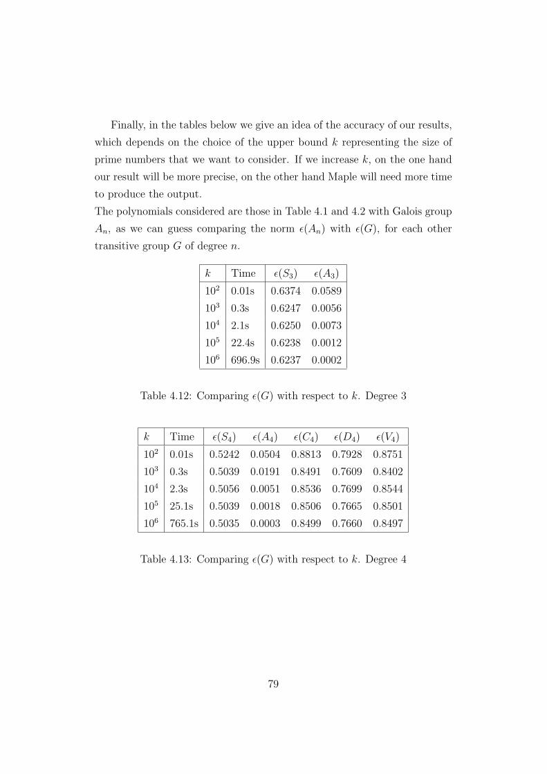
Finally, in the tables below we give an idea of the accuracy of our results,
which depends on the choice of the upper bound k representing the size of
prime numbers that we want to consider. If we increase k, on the one hand
our result will be more precise, on the other hand Maple will need more time
to produce the output.
The polynomials considered are those in Table 4.1 and 4.2 with Galois group
An, as we can guess comparing the norm ε(An) with ε(G), for each other
transitive group G of degree n.
k Time ε(S3) ε(A3)
102 0.01s 0.6374 0.0589
103 0.3s 0.6247 0.0056
104 2.1s 0.6250 0.0073
105 22.4s 0.6238 0.0012
106 696.9s 0.6237 0.0002
Table 4.12: Comparing ε(G) with respect to k. Degree 3
k Time ε(S4) ε(A4) ε(C4) ε(D4) ε(V4)
102 0.01s 0.5242 0.0504 0.8813 0.7928 0.8751
103 0.3s 0.5039 0.0191 0.8491 0.7609 0.8402
104 2.3s 0.5056 0.0051 0.8536 0.7699 0.8544
105 25.1s 0.5039 0.0018 0.8506 0.7665 0.8501
106 765.1s 0.5035 0.0003 0.8499 0.7660 0.8497
Table 4.13: Comparing ε(G) with respect to k. Degree 4
79

k Time ε(S5) ε(A5) ε(F20) ε(D5) ε(C5)
102 0.01s 0.4582 0.1114 0.6758 0.4934 0.5429
103 0.3s 0.4289 0.0325 0.6281 0.3993 0.6014
104 2.2s 0.4254 0.0321 0.6396 0.4413 0.6360
105 24.8s 0.4255 0.0023 0.6341 0.4239 0.6044
106 700.3s 0.4252 0.0008 0.6343 0.4248 0.6054
Table 4.14: Comparing ε(G) with respect to k. Degree 5
k Time ε(S6) ε(A6) ε(PGL2(F5)) ε(G72)
102 0.01s 0.4977 0.2516 0.6212 0.5791
103 0.3s 0.3906 0.0696 0.4796 0.5184
104 2.9s 0.3691 0.0189 0.4647 0.4787
105 30.8s 0.3725 0.0038 0.4654 0.4879
106 948.4s 0.3710 0.0016 0.4641 0.4848
k Time ε(PSL2(F5)) ε(G48) ε(G236) ε(G1
36)
102 0.01s 0.5699 0.6513 0.5304 0.7738
103 0.3s 0.3808 0.5449 0.5291 0.6519
104 2.9s 0.3807 0.5095 0.4785 0.6131
105 30.8s 0.3754 0.5164 0.4914 0.6171
106 948.4s 0.3750 0.5133 0.4874 0.6145
Table 4.15: (A) Comparing ε(G) with respect to k. Degree 6.
80

k Time ε(S4−) ε(S4+) ε(G24) ε(G18)
102 0.01s 0.8057 0.6706 0.8079 0.8126
103 0.3s 0.6552 0.5719 0.6578 0.6501
104 2.9s 0.6364 0.5296 0.6391 0.6287
105 30.8s 0.6433 0.5379 0.6459 0.6382
106 948.4s 0.6407 0.5340 0.6434 0.6358
k Time ε(A4) ε(D6) ε(S3) ε(C6)
102 0.01s 0.9412 0.7797 0.8991 0.8350
103 0.3s 0.7602 0.6636 0.7635 0.6869
104 2.9s 0.7466 0.6309 0.7544 0.6768
105 30.8s 0.7548 0.6341 0.7613 0.6844
106 948.4s 0.7519 0.6316 0.7591 0.6821
Table 4.16: (B) Comparing ε(G) with respect to k. Degree 6
k Time ε(S7) ε(A7) ε(PSL2(F7))
102 0.01s 0.3459 0.1069 0.3172
103 0.3s 0.3280 0.0346 0.3475
104 3.4s 0.3267 0.0131 0.3200
105 33.5s 0.3269 0.0113 0.3234
106 950.2s 0.3248 0.0036 0.3255
Table 4.17: (A) Comparing ε(G) with respect to k. Degree 7.
81

k Time ε(F42) ε(F21) ε(D7) ε(C7)
102 0.01s 0.5741 0.6499 0.5918 0.5957
103 0.3s 0.5776 0.6666 0.6436 0.7049
104 3.4s 0.5675 0.6496 0.6273 0.6753
105 33.5s 0.5672 0.6488 0.6288 0.6778
106 950.2s 0.5679 0.6519 0.6318 0.6853
Table 4.18: (B) Comparing ε(G) with respect to k. Degree 7.
k Time ε(S11) ε(A11) ε(M11) ε(PSL2(F11))
102 0.3s 0.3428 0.2399 0.4033 0.4465
103 1.3s 0.2309 0.0769 0.3269 0.4521
104 9.2s 0.2149 0.0278 0.3232 0.4767
105 94.1s 0.2133 0.0093 0.3257 0.4775
106 1878s 0.2128 0.0034 0.3268 0.4770
k Time ε(F110) ε(F55) ε(D11) ε(C11)
102 0.3s 0.6208 0.7680 0.5892 0.6587
103 1.3s 0.5959 0.7784 0.6183 0.7622
104 9.2s 0.6075 0.8018 0.6206 0.7718
105 94.1s 0.6037 0.7965 0.6190 0.7698
106 1878s 0.6036 0.7966 0.6204 0.7722
Table 4.19: Comparing ε(G) with respect to k.
82
The norm ε(G) can be regarded as a measure of the distance between the
theoretical and the empirical result.
Definition 4.1.5. We call ε(G) the relative error of G.
It’s clear that ε(G) = ε(G, k). From the analysis of the relative errors we
notice that
ε(An, 106) < 10−2 and ε(An, 103) < 10−1,
and, by induction, one may naively guess ε(G, 103t) < 10−t, t ≥ 1, where G
equals Gal(f). This observation shows that k ≥ 103 usually is a good bound
for the Chebotarev test.
4.2 Groups of Prime Degree Polynomials
Computing Galois groups is still a difficult task. Even with the devel-
opment of new computer algebra systems this remains a challenge and can
be accomplished only for small degree polynomials. For example, Maple9
can only handle polynomials of degree ≤ 9 and GP/Pari up to degree 11.
Other computer algebra packages can handle polynomials whose degree is in
the same range. The existence of non–real roots of a polynomial makes the
computation of its Galois group much easier. Computing the Galois group
in this case, for polynomials of prime degree p, will be the focus of this
section. Checking whether a polynomial has non–real roots is very efficient
since numerical methods can be used. Once the existence of non–real roots
is established then from a theorem of Jordan (1871) it follows that if their
number is small enough with respect to the degree p of the polynomial, then
the Galois group is Ap or Sp. Furthermore, knowledge of the complete classi-
fication of transitive groups of prime degree enables us to provide a complete
list of possible Galois groups for every irreducible polynomial of prime degree
p which has non–real roots.
By degree of a permutation group G ⊆ Sn we mean the number of points
in 1, . . . , n moved by G. The degree of a permutation α ∈ Sn is the number
83
of points moved by 〈α〉. The minimal degree of G, denoted by m(G), is the
smallest of degrees of elements α 6= 1 in G. Let f(x) ∈ Q[x] be an irreducible
polynomial of degree n ≥ 5. Denote by r the number of non-real roots of
f(x). Since the complex conjugation permutes the roots then r is even, say
r = 2s, by a reordering of the roots and we may assume that if f(x) has r
non–real roots then
α := (1, 2)(3, 4) · · · (r − 1, r) ∈ Gal(f)
is the complex conjugation Since determining the number of non–real roots
can be very fast, we would like to know to what extent the number of non–
real roots of f(x) determines Gal(f). The complex conjugation assures that
m(G) ≤ r. The existence of α can narrow down the list of candidates for
Gal(f).
Example 4.2.1. Let f(x) = 48x7 − 56x6 + 7 be an irreducible polynomial.
From a simple computation we discover that the number of real roots of f(x)
is 3, and so there exists an elemente α ∈ Gal(f) of the form (1, 2)(3, 4),
which permutes 4 complex roots of f(x).
Looking at the Table 3.9 of transitive group of order 7, we find that possible
candidates for Gal(f) are S7, A7, PSL2(F7). Then one can use other tools,
like computation of ∆(f) and mod p reductions, to determine this group uni-
vocally.
In despite of the example above, it is unlikely that the group can be
determined only from this information unless p is ”large” enough. In this
case the number of non–real roots of f(x) can almost determine the Galois
group of f(x), as we will see. Nevertheless, the test is worth running for all
p since it is very fast and improves the algorithm overall.
Next theorem determines the Galois group of a prime degree polynomial f(x)
with r non–real roots when the degree of f(x) is large enough with respect
to r. We refer to [Ser03] for a more extensive description of the following
results.
84

Theorem 4.2.2. Let f(x) ∈ Q[x] be an irreducible polynomial of prime
degree p ≥ 3 and r = 2s be the number of non–real roots of f(x). If s
satisfies
s(slogs + 2logs + 3) ≤ p
then Gal(f) = Ap, or Sp.
Proof. Since p is prime, every transitive subgroup of Sp is primitive (see [Rot95]).
Let G denote the Galois group of f(x) and m(G) its minimal degree. By re-
ordering the roots we can assume that
(1, 2)(3, 4) · · · (r − 1, r) ∈ Gal(f).
Hence, m := m(G) ≤ r. From the theorem of Jordan discussed in [Jor72] we
have that
m2
4log
m
2+ m
(log
m
2+
3
2
)≤ p ⇒ G = Ap or Sp.
Hence, if we consider r = 2s instead of m, we have that if
s(slogs + 2logs + 3) ≤ p
then G = Ap or Sp.
For a fixed p the above bound is not sharp as we will see below. However,
Theorem 4.2.2 can be used successfully if s is fixed. We denote the above
lower bound on p by N(r) := [s(slogs + 2logs + 3)] for r = 2s. Hence, for a
fixed number of non–real roots and for p ≥ N(r) the Galois group is always
Ap or Sp.
Corollary 4.2.3. Let a polynomial of prime degree p and assume that r
denotes the number of its non-real roots. If one of the following holds:
(i) r = 2 and p > 2,
(ii) r = 4 and p > 7,
(iii) r = 6 and p > 13,
85
(iv) r = 8 and p > 23,
(v) r = 10 and p > 37,
then Gal(f) = Ap or Sp.
Remark 4.2.4. The above results gives a very quick way of determining
the Galois group for polynomials with non–real roots. Whether or not the
discriminant is a complete square can be used to distinguish between Ap and
Sp. In the case (i), (iii), (v), it’s very easy to choose between Ap and Sp; in
fact we have obviously that Gal(f) = Sp, since the complex conjugation is an
odd permutation.
If p < N(r) then some exceptional cases occur. We remark that if we
consider f(x) such that ∂f = p ≤ 29, no two groups have the same cycle
structure, and so the Galois group can be determined uniquely by reduction
modulo p for all polynomials of prime degree ≤ 29 with non–real roots.
Example 4.2.5. Let f(x) = x7−4x6−20x5+4x4+20x3+2. This polynomial
is irreducible over Q and has exactly 2 non–real roots. We can easily check
these facts in Maple9 using the commands
f:=x^7-4*x^6-20*x^5+4*x^4+20*x^3+2;
factor(f);
realroot(f);
From Corollary 4.2.3, Gal(f) is S7 or A7. Its discriminant is ∆(f) = −(2)6 ·(3)3 · (47031541) · (4289), which is ≤ 0; therefore it is not a square in Q and
the Galois group of f(x) is S7, as we can verify with the command
galois(x^7-4*x^6-20*x^5+4*x^4+20*x^3+2);
"7T7", "S(7)", "-", 5040;
Combining the above results we have the following algorithm for comput-
ing the Galois group of prime degree polynomials with non–real roots. Note
that even in the case p < N(r) we know that a permutation of the type (2)r2
86
is in the group. Hence, the list of transitive subgroups is much shorter than
in general. This information was obtained by computing the number of real
roots rather then by some factorization modulo p. Thus, even in this case
the algorithm can be improved.
Algorithm: Computing the Galois group of prime degree polynomials with
few non–real roots.
Input: an irreducible monic polynomial f(x) ∈ Z[x] of prime degree p.
Output: Galois group of f(x) over Q.
begin
r:=Number Of Real Roots(f(x));
if p > N(r)
if D(f) is a square
Gal(f)=A_p;
else Gal(f) = S_p;
else Chebotarev test(f(x));
end;
Example 4.2.6. Let f(x) = x11 +4x10−14x9−56x8 +50x7 +200x6−50x5−200x4 + 49x3 + 196x2 − 36x− 143 be irreducible over Q. We get
nops(realroot(f));
7
In fact f(x) has been produced expanding (x4+1)(x+4)∏3
j=1(x±j)+1, which
is proved to be irreducible. In this case r = 11 − 7 = 4 and N(r) ≈ 8.41,
which is ≤ p = 11. We are in the conditions of Corollary 4.2.3, hence
Gal(f) = S11 or A11. Computing discriminant we observe that it’s not a
square and therefore
Gal(f) * A11 ⇒ Gal(f) = S11.
87

Appendix A
Roots on Finite Fields
In this appendix we study the form of the roots of an irreducible polyno-
mial in a finite fields of characteristic q. The following results are from [LN94].
Theorem A.0.7. Let f(x) ∈ Fq[x] be an irreducible polynomial of degree m;
then f(x) has a root in Fqm. Moreover, if f(α) = 0, all the m distinct roots
of f have molteplicity 1 and they are of the form
αqh ∈ Fqm , for all 0 ≤ h ≤ m− 1.
Proof. Let α be such that f(α) = 0; then [Fq(α) : Fq] = m, i.e. Fq(α) ' Fqm
and we can consider α as an element in Fqm . We will show that f(β) = 0
implies (βq), for any β ∈ Fqm . Let f(x) =∑m
i=0 aixi, ai ∈ Fq; then
f(βq) = amβqm + am−1βq(m−1) + · · ·+ a1β
q + a0
= aqmβqm + aq
m−1βq(m−1) + · · ·+ aq
1βq + aq
0
= (amβm + am−1βm−1 + · · ·+ a1β + a0)
q
= [f(β)]q
= 0.
From this observation we conclude that if α is a root, then αp, αp2, . . . , αqm−1
are roots of f . We will show that these roots are distinct. If there exist j, k
such that αqj= αqk
, with 0 ≤ j < k ≤ m − 1, then αqj+m−k= αqm
and
88
therefore αqj+m−k= α, that is, α is a root of xqj+m−k −x. Hence f(x) must di
divide xqj+m−k−x, but from Lemma A.0.8 f |xqj+m−k−x ⇔ ∂f = m|m−j+k.
Now, 0 < m− k + j < m, and if m|m− k + j we have an absurd.
Lemma A.0.8. Let f(x) ∈ Fq[x] be an irreducible polynomial of degree m;
then f(x)|xqn − x ⇔ ∂f = m|n.
Proof. (⇒) We assume that f(x)|xqn − x; let α be a root of f(x); then
αqn= α ⇔ α ∈ Fqn ⇔ Fq(α) ⊆ Fqn . But [Fq(α) : Fq] = m and [Fn
q : Fq] = n
imply that n = [Fnq : Fq(α)] ·m, and so m|n.
(⇐) It is easily seen that m|n ⇔ Fqn ⊃ Fqm . If α is a root of f(x), then
[Fq(α) : Fq] = m, and therefore Fq(α) = Fqm ⊂ Fqn . So α ∈ Fqn or, in
other words, αqn= α, that is, α is a root of xqn − x ∈ Fq[x]. In short,
f(x)|xqn − x.
89
Appendix B
Galois Groups on Finite Fields
Let Fp = Z/pZ, the field of p elements. Any other field E of characteristic
p contains a copy of Fp, namely, m1E : m ∈ Z. No harm results if we
identify Fp with this subfield of E. Let E be a field of degree n over Fp.
Then E has q = pn elements, and so E∗ = E −0 is a group of order q− 1.
Hence the nonzero elements of E are roots xq−1 − 1, and all elements of E,
including 0, are roots of xq − x. Hence E is a splitting field for xq − x, and
so any two fields with q elements are isomorphic.
Now let E be the splitting field of f(x) = xq − x, q = pn. The formal
derivative f ′(x) ≡ −1 mod p is relatively prime to f(x) and so f(x) has q
distinct roots in E. Let S be the set of its roots. Then S is obviously closed
under multiplication and the formation of inverses, but it is also closed under
subtraction; if aq = a and bq = b, then
(a− b)q = aq − bq = a− b.
Hence S is a field, and so S = E. In particular, E has pn elements.
Proposition B.0.9. For each power q = pn there is a field Fq with q ele-
ments. It is the splitting field of xq − x, and hence any two such fields are
isomorphic. Moreover, Fq is Galois over Fp with cyclic Galois group gener-
ated by the Frobenius automorphism σ : a 7→ ap.
90
Proof. The field Fq is Galois over Fp because it is the splitting field of a
separable polynomial f(x), namely xq − x. We noted that σ : x 7→ xp is
an automorphism of Fq, sending each root f(x) into another one, for Theo-
rem A.0.7. An element a ∈ Fq is fixed by σ if and only if ap = a; but Fp
consists exactly of such elements, and so the fixed field of 〈σ〉 is Fp. This
proves that Fq is Galois over Fp and that 〈σ〉 = Gal(Fq/Fp).
91
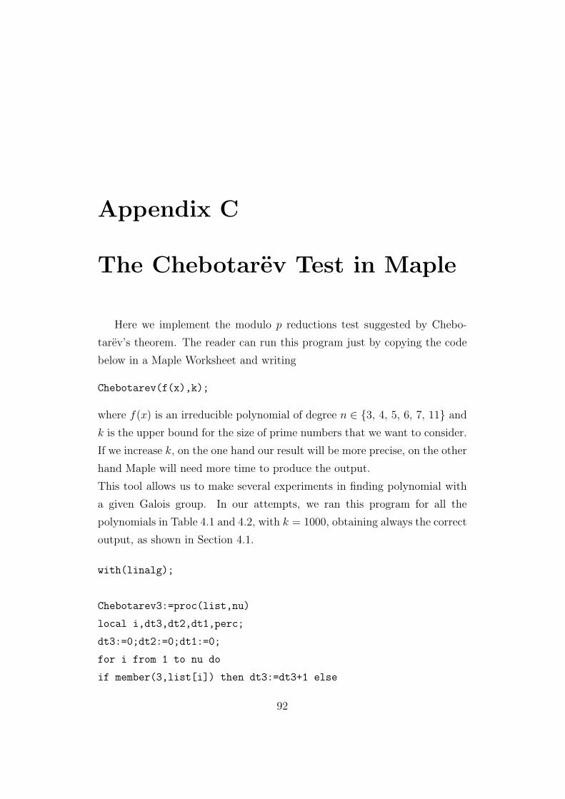
Appendix C
The Chebotarev Test in Maple
Here we implement the modulo p reductions test suggested by Chebo-
tarev’s theorem. The reader can run this program just by copying the code
below in a Maple Worksheet and writing
Chebotarev(f(x),k);
where f(x) is an irreducible polynomial of degree n ∈ 3, 4, 5, 6, 7, 11 and
k is the upper bound for the size of prime numbers that we want to consider.
If we increase k, on the one hand our result will be more precise, on the other
hand Maple will need more time to produce the output.
This tool allows us to make several experiments in finding polynomial with
a given Galois group. In our attempts, we ran this program for all the
polynomials in Table 4.1 and 4.2, with k = 1000, obtaining always the correct
output, as shown in Section 4.1.
with(linalg);
Chebotarev3:=proc(list,nu)
local i,dt3,dt2,dt1,perc;
dt3:=0;dt2:=0;dt1:=0;
for i from 1 to nu do
if member(3,list[i]) then dt3:=dt3+1 else
92
if verify(list[i],[0,1,2],sublist) then dt2:=dt2+1 else
if verify(list[i],[0,1,1,1],sublist) then dt1:=dt1+1 fi;
fi;fi;
od;
print((0,0,3)=dt3/nu);
print((0,1,2)=dt2/nu);
print((1,1,1)=dt1/nu);
perc:=array(1..nu,[dt1/nu,dt2/nu,dt3/nu]);
getGroup3(perc);
end:
getGroup3:=proc(a)
local i,b,c;
c:=array(1..3,[1/3,0 ,2/3]);
b:=array(1..3,[1/6,1/2,1/3]);
for i from 1 to 3 do
b[i]:=a[i]-b[i];c[i]:=a[i]-c[i];
od;
if evalf(norm(c,frobenius))<evalf(norm(b,frobenius)) then
print("Gruppo A(3)") else print("Gruppo S(3)") fi;
end:
Chebotarev4:=proc(list,nu)
local i,dt5,dt4,dt3,dt2,dt1,perc;
dt5:=0;dt4:=0;dt3:=0;dt2:=0;dt1:=0;
for i from 1 to nu do
if member(4,list[i]) then dt5:=dt5+1 else
if verify(list[i],[0,1,3],sublist) then dt4:=dt4+1 else
if verify(list[i],[0,2,2],sublist) then dt3:=dt3+1 else
if verify(list[i],[0,1,1,2],sublist) then dt2:=dt2+1 else
93
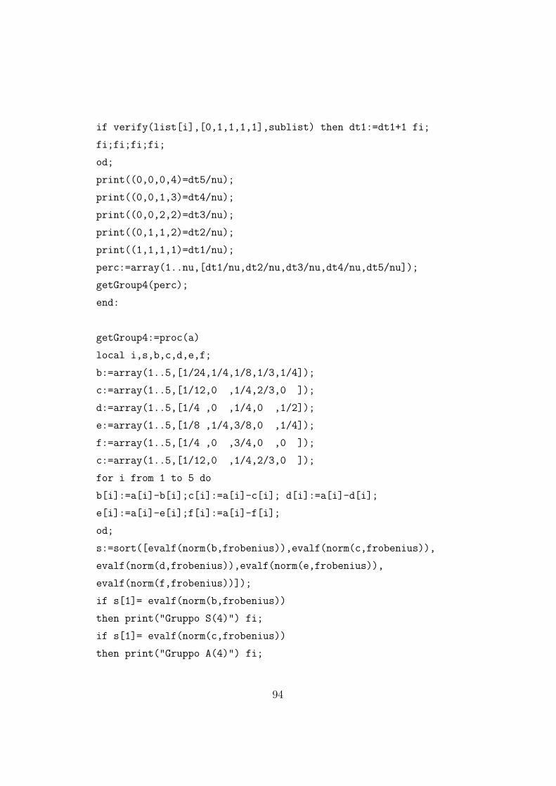
if verify(list[i],[0,1,1,1,1],sublist) then dt1:=dt1+1 fi;
fi;fi;fi;fi;
od;
print((0,0,0,4)=dt5/nu);
print((0,0,1,3)=dt4/nu);
print((0,0,2,2)=dt3/nu);
print((0,1,1,2)=dt2/nu);
print((1,1,1,1)=dt1/nu);
perc:=array(1..nu,[dt1/nu,dt2/nu,dt3/nu,dt4/nu,dt5/nu]);
getGroup4(perc);
end:
getGroup4:=proc(a)
local i,s,b,c,d,e,f;
b:=array(1..5,[1/24,1/4,1/8,1/3,1/4]);
c:=array(1..5,[1/12,0 ,1/4,2/3,0 ]);
d:=array(1..5,[1/4 ,0 ,1/4,0 ,1/2]);
e:=array(1..5,[1/8 ,1/4,3/8,0 ,1/4]);
f:=array(1..5,[1/4 ,0 ,3/4,0 ,0 ]);
c:=array(1..5,[1/12,0 ,1/4,2/3,0 ]);
for i from 1 to 5 do
b[i]:=a[i]-b[i];c[i]:=a[i]-c[i]; d[i]:=a[i]-d[i];
e[i]:=a[i]-e[i];f[i]:=a[i]-f[i];
od;
s:=sort([evalf(norm(b,frobenius)),evalf(norm(c,frobenius)),
evalf(norm(d,frobenius)),evalf(norm(e,frobenius)),
evalf(norm(f,frobenius))]);
if s[1]= evalf(norm(b,frobenius))
then print("Gruppo S(4)") fi;
if s[1]= evalf(norm(c,frobenius))
then print("Gruppo A(4)") fi;
94
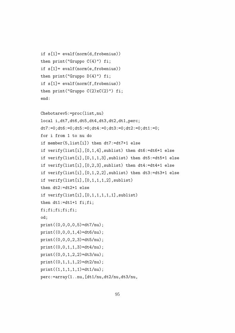
if s[1]= evalf(norm(d,frobenius))
then print("Gruppo C(4)") fi;
if s[1]= evalf(norm(e,frobenius))
then print("Gruppo D(4)") fi;
if s[1]= evalf(norm(f,frobenius))
then print("Gruppo C(2)xC(2)") fi;
end:
Chebotarev5:=proc(list,nu)
local i,dt7,dt6,dt5,dt4,dt3,dt2,dt1,perc;
dt7:=0;dt6:=0;dt5:=0;dt4:=0;dt3:=0;dt2:=0;dt1:=0;
for i from 1 to nu do
if member(5,list[i]) then dt7:=dt7+1 else
if verify(list[i],[0,1,4],sublist) then dt6:=dt6+1 else
if verify(list[i],[0,1,1,3],sublist) then dt5:=dt5+1 else
if verify(list[i],[0,2,3],sublist) then dt4:=dt4+1 else
if verify(list[i],[0,1,2,2],sublist) then dt3:=dt3+1 else
if verify(list[i],[0,1,1,1,2],sublist)
then dt2:=dt2+1 else
if verify(list[i],[0,1,1,1,1,1],sublist)
then dt1:=dt1+1 fi;fi;
fi;fi;fi;fi;fi;
od;
print((0,0,0,0,5)=dt7/nu);
print((0,0,0,1,4)=dt6/nu);
print((0,0,0,2,3)=dt5/nu);
print((0,0,1,1,3)=dt4/nu);
print((0,0,1,2,2)=dt3/nu);
print((0,1,1,1,2)=dt2/nu);
print((1,1,1,1,1)=dt1/nu);
perc:=array(1..nu,[dt1/nu,dt2/nu,dt3/nu,
95
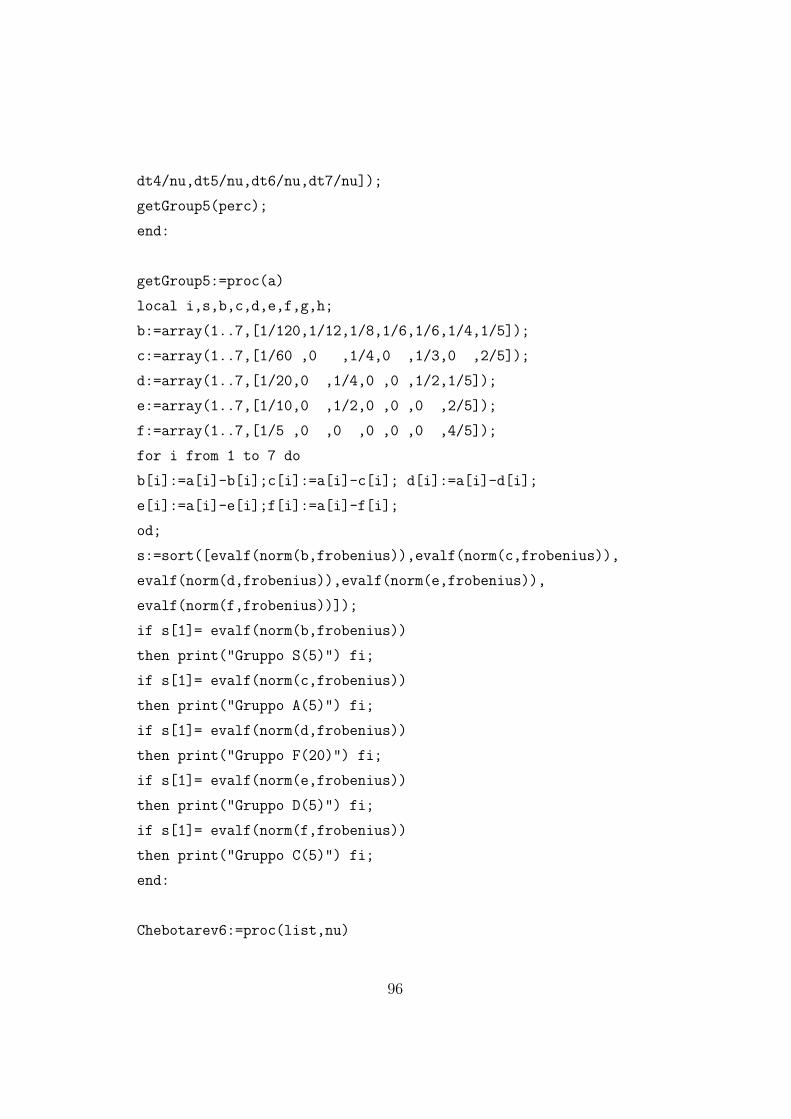
dt4/nu,dt5/nu,dt6/nu,dt7/nu]);
getGroup5(perc);
end:
getGroup5:=proc(a)
local i,s,b,c,d,e,f,g,h;
b:=array(1..7,[1/120,1/12,1/8,1/6,1/6,1/4,1/5]);
c:=array(1..7,[1/60 ,0 ,1/4,0 ,1/3,0 ,2/5]);
d:=array(1..7,[1/20,0 ,1/4,0 ,0 ,1/2,1/5]);
e:=array(1..7,[1/10,0 ,1/2,0 ,0 ,0 ,2/5]);
f:=array(1..7,[1/5 ,0 ,0 ,0 ,0 ,0 ,4/5]);
for i from 1 to 7 do
b[i]:=a[i]-b[i];c[i]:=a[i]-c[i]; d[i]:=a[i]-d[i];
e[i]:=a[i]-e[i];f[i]:=a[i]-f[i];
od;
s:=sort([evalf(norm(b,frobenius)),evalf(norm(c,frobenius)),
evalf(norm(d,frobenius)),evalf(norm(e,frobenius)),
evalf(norm(f,frobenius))]);
if s[1]= evalf(norm(b,frobenius))
then print("Gruppo S(5)") fi;
if s[1]= evalf(norm(c,frobenius))
then print("Gruppo A(5)") fi;
if s[1]= evalf(norm(d,frobenius))
then print("Gruppo F(20)") fi;
if s[1]= evalf(norm(e,frobenius))
then print("Gruppo D(5)") fi;
if s[1]= evalf(norm(f,frobenius))
then print("Gruppo C(5)") fi;
end:
Chebotarev6:=proc(list,nu)
96
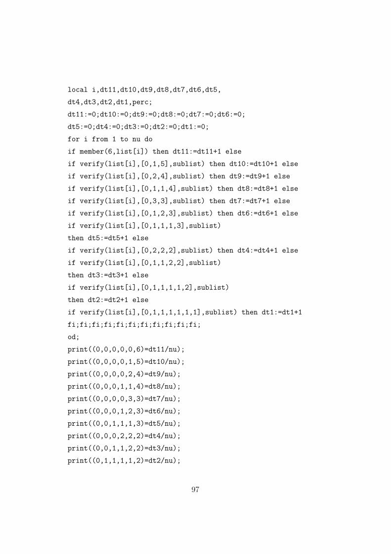
local i,dt11,dt10,dt9,dt8,dt7,dt6,dt5,
dt4,dt3,dt2,dt1,perc;
dt11:=0;dt10:=0;dt9:=0;dt8:=0;dt7:=0;dt6:=0;
dt5:=0;dt4:=0;dt3:=0;dt2:=0;dt1:=0;
for i from 1 to nu do
if member(6,list[i]) then dt11:=dt11+1 else
if verify(list[i],[0,1,5],sublist) then dt10:=dt10+1 else
if verify(list[i],[0,2,4],sublist) then dt9:=dt9+1 else
if verify(list[i],[0,1,1,4],sublist) then dt8:=dt8+1 else
if verify(list[i],[0,3,3],sublist) then dt7:=dt7+1 else
if verify(list[i],[0,1,2,3],sublist) then dt6:=dt6+1 else
if verify(list[i],[0,1,1,1,3],sublist)
then dt5:=dt5+1 else
if verify(list[i],[0,2,2,2],sublist) then dt4:=dt4+1 else
if verify(list[i],[0,1,1,2,2],sublist)
then dt3:=dt3+1 else
if verify(list[i],[0,1,1,1,1,2],sublist)
then dt2:=dt2+1 else
if verify(list[i],[0,1,1,1,1,1,1],sublist) then dt1:=dt1+1
fi;fi;fi;fi;fi;fi;fi;fi;fi;fi;fi;
od;
print((0,0,0,0,0,6)=dt11/nu);
print((0,0,0,0,1,5)=dt10/nu);
print((0,0,0,0,2,4)=dt9/nu);
print((0,0,0,1,1,4)=dt8/nu);
print((0,0,0,0,3,3)=dt7/nu);
print((0,0,0,1,2,3)=dt6/nu);
print((0,0,1,1,1,3)=dt5/nu);
print((0,0,0,2,2,2)=dt4/nu);
print((0,0,1,1,2,2)=dt3/nu);
print((0,1,1,1,1,2)=dt2/nu);
97
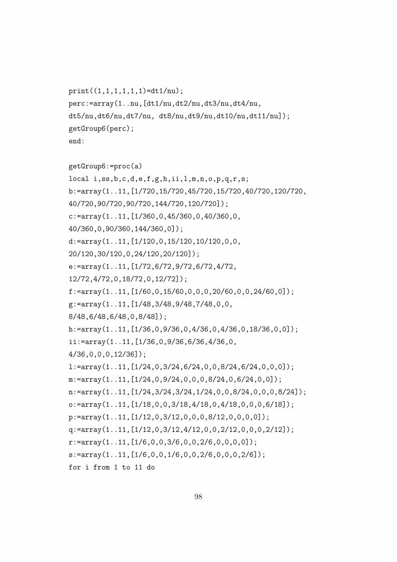
print((1,1,1,1,1,1)=dt1/nu);
perc:=array(1..nu,[dt1/nu,dt2/nu,dt3/nu,dt4/nu,
dt5/nu,dt6/nu,dt7/nu, dt8/nu,dt9/nu,dt10/nu,dt11/nu]);
getGroup6(perc);
end:
getGroup6:=proc(a)
local i,ss,b,c,d,e,f,g,h,ii,l,m,n,o,p,q,r,s;
b:=array(1..11,[1/720,15/720,45/720,15/720,40/720,120/720,
40/720,90/720,90/720,144/720,120/720]);
c:=array(1..11,[1/360,0,45/360,0,40/360,0,
40/360,0,90/360,144/360,0]);
d:=array(1..11,[1/120,0,15/120,10/120,0,0,
20/120,30/120,0,24/120,20/120]);
e:=array(1..11,[1/72,6/72,9/72,6/72,4/72,
12/72,4/72,0,18/72,0,12/72]);
f:=array(1..11,[1/60,0,15/60,0,0,0,20/60,0,0,24/60,0]);
g:=array(1..11,[1/48,3/48,9/48,7/48,0,0,
8/48,6/48,6/48,0,8/48]);
h:=array(1..11,[1/36,0,9/36,0,4/36,0,4/36,0,18/36,0,0]);
ii:=array(1..11,[1/36,0,9/36,6/36,4/36,0,
4/36,0,0,0,12/36]);
l:=array(1..11,[1/24,0,3/24,6/24,0,0,8/24,6/24,0,0,0]);
m:=array(1..11,[1/24,0,9/24,0,0,0,8/24,0,6/24,0,0]);
n:=array(1..11,[1/24,3/24,3/24,1/24,0,0,8/24,0,0,0,8/24]);
o:=array(1..11,[1/18,0,0,3/18,4/18,0,4/18,0,0,0,6/18]);
p:=array(1..11,[1/12,0,3/12,0,0,0,8/12,0,0,0,0]);
q:=array(1..11,[1/12,0,3/12,4/12,0,0,2/12,0,0,0,2/12]);
r:=array(1..11,[1/6,0,0,3/6,0,0,2/6,0,0,0,0]);
s:=array(1..11,[1/6,0,0,1/6,0,0,2/6,0,0,0,2/6]);
for i from 1 to 11 do
98

b[i]:=a[i]-b[i];c[i]:=a[i]-c[i]; d[i]:=a[i]-d[i];
e[i]:=a[i]-e[i];f[i]:=a[i]-f[i]; g[i]:=a[i]-g[i];
h[i]:=a[i]-h[i];ii[i]:=a[i]-ii[i];l[i]:=a[i]-l[i];
m[i]:=a[i]-m[i];n[i]:=a[i]-n[i];o[i]:=a[i]-o[i];
p[i]:=a[i]-p[i];q[i]:=a[i]-q[i];r[i]:=a[i]-r[i];
s[i]:=a[i]-s[i];
od;
ss:=sort([evalf(norm(b,frobenius)),
evalf(norm(c,frobenius)),
evalf(norm(d,frobenius)),evalf(norm(e,frobenius)),
evalf(norm(f,frobenius)),evalf(norm(g,frobenius)),
evalf(norm(h,frobenius)),evalf(norm(ii,frobenius)),
evalf(norm(l,frobenius)),evalf(norm(m,frobenius)),
evalf(norm(n,frobenius)),evalf(norm(o,frobenius)),
evalf(norm(p,frobenius)),evalf(norm(q,frobenius)),
evalf(norm(r,frobenius)),evalf(norm(s,frobenius))]);
if ss[1]= evalf(norm(b,frobenius))
then print("Gruppo S(6)") fi;
if ss[1]= evalf(norm(c,frobenius))
then print("Gruppo A(6)") fi;
if ss[1]= evalf(norm(d,frobenius))
then print("Gruppo PGL(2,5)") fi;
if ss[1]= evalf(norm(e,frobenius))
then print("Gruppo G(72)") fi;
if ss[1]= evalf(norm(f,frobenius))
then print("Gruppo PSL(2,5)") fi;
if ss[1]= evalf(norm(g,frobenius))
then print("Gruppo G(48)") fi;
if ss[1]= evalf(norm(h,frobenius))
then print("Gruppo G2(36)") fi;
if ss[1]= evalf(norm(ii,frobenius))
99
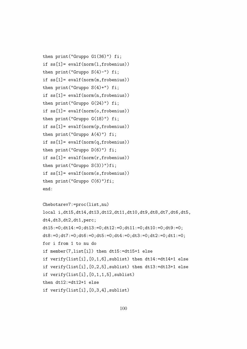
then print("Gruppo G1(36)") fi;
if ss[1]= evalf(norm(l,frobenius))
then print("Gruppo S(4)-") fi;
if ss[1]= evalf(norm(m,frobenius))
then print("Gruppo S(4)+") fi;
if ss[1]= evalf(norm(n,frobenius))
then print("Gruppo G(24)") fi;
if ss[1]= evalf(norm(o,frobenius))
then print("Gruppo G(18)") fi;
if ss[1]= evalf(norm(p,frobenius))
then print("Gruppo A(4)") fi;
if ss[1]= evalf(norm(q,frobenius))
then print("Gruppo D(6)") fi;
if ss[1]= evalf(norm(r,frobenius))
then print("Gruppo S(3))")fi;
if ss[1]= evalf(norm(s,frobenius))
then print("Gruppo C(6)")fi;
end:
Chebotarev7:=proc(list,nu)
local i,dt15,dt14,dt13,dt12,dt11,dt10,dt9,dt8,dt7,dt6,dt5,
dt4,dt3,dt2,dt1,perc;
dt15:=0;dt14:=0;dt13:=0;dt12:=0;dt11:=0;dt10:=0;dt9:=0;
dt8:=0;dt7:=0;dt6:=0;dt5:=0;dt4:=0;dt3:=0;dt2:=0;dt1:=0;
for i from 1 to nu do
if member(7,list[i]) then dt15:=dt15+1 else
if verify(list[i],[0,1,6],sublist) then dt14:=dt14+1 else
if verify(list[i],[0,2,5],sublist) then dt13:=dt13+1 else
if verify(list[i],[0,1,1,5],sublist)
then dt12:=dt12+1 else
if verify(list[i],[0,3,4],sublist)
100
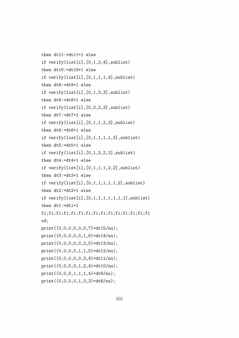
then dt11:=dt11+1 else
if verify(list[i],[0,1,2,4],sublist)
then dt10:=dt10+1 else
if verify(list[i],[0,1,1,1,4],sublist)
then dt9:=dt9+1 else
if verify(list[i],[0,1,3,3],sublist)
then dt8:=dt8+1 else
if verify(list[i],[0,2,2,3],sublist)
then dt7:=dt7+1 else
if verify(list[i],[0,1,1,2,3],sublist)
then dt6:=dt6+1 else
if verify(list[i],[0,1,1,1,1,3],sublist)
then dt5:=dt5+1 else
if verify(list[i],[0,1,2,2,2],sublist)
then dt4:=dt4+1 else
if verify(list[i],[0,1,1,1,2,2],sublist)
then dt3:=dt3+1 else
if verify(list[i],[0,1,1,1,1,1,2],sublist)
then dt2:=dt2+1 else
if verify(list[i],[0,1,1,1,1,1,1,1],sublist)
then dt1:=dt1+1
fi;fi;fi;fi;fi;fi;fi;fi;fi;fi;fi;fi;fi;fi;fi
od;
print((0,0,0,0,0,0,7)=dt15/nu);
print((0,0,0,0,0,1,6)=dt14/nu);
print((0,0,0,0,0,2,5)=dt13/nu);
print((0,0,0,0,1,1,5)=dt12/nu);
print((0,0,0,0,0,3,4)=dt11/nu);
print((0,0,0,0,1,2,4)=dt10/nu);
print((0,0,0,1,1,1,4)=dt9/nu);
print((0,0,0,0,1,3,3)=dt8/nu);
101
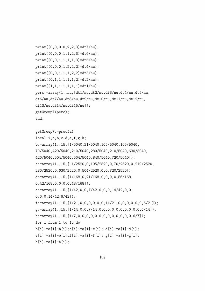
print((0,0,0,0,2,2,3)=dt7/nu);
print((0,0,0,1,1,2,3)=dt6/nu);
print((0,0,1,1,1,1,3)=dt5/nu);
print((0,0,0,1,2,2,2)=dt4/nu);
print((0,0,1,1,1,2,2)=dt3/nu);
print((0,1,1,1,1,1,2)=dt2/nu);
print((1,1,1,1,1,1,1)=dt1/nu);
perc:=array(1..nu,[dt1/nu,dt2/nu,dt3/nu,dt4/nu,dt5/nu,
dt6/nu,dt7/nu,dt8/nu,dt9/nu,dt10/nu,dt11/nu,dt12/nu,
dt13/nu,dt14/nu,dt15/nu]);
getGroup7(perc);
end:
getGroup7:=proc(a)
local i,s,b,c,d,e,f,g,h;
b:=array(1..15,[1/5040,21/5040,105/5040,105/5040,
70/5040,420/5040,210/5040,280/5040,210/5040,630/5040,
420/5040,504/5040,504/5040,840/5040,720/5040]);
c:=array(1..15,[ 1/2520,0,105/2520,0,70/2520,0,210/2520,
280/2520,0,630/2520,0,504/2520,0,0,720/2520]);
d:=array(1..15,[1/168,0,21/168,0,0,0,0,56/168,
0,42/168,0,0,0,0,48/168]);
e:=array(1..15,[1/42,0,0,7/42,0,0,0,14/42,0,0,
0,0,0,14/42,6/42]);
f:=array(1..15,[1/21,0,0,0,0,0,0,14/21,0,0,0,0,0,0,6/21]);
g:=array(1..15,[1/14,0,0,7/14,0,0,0,0,0,0,0,0,0,0,6/14]);
h:=array(1..15,[1/7,0,0,0,0,0,0,0,0,0,0,0,0,0,6/7]);
for i from 1 to 15 do
b[i]:=a[i]-b[i];c[i]:=a[i]-c[i]; d[i]:=a[i]-d[i];
e[i]:=a[i]-e[i];f[i]:=a[i]-f[i]; g[i]:=a[i]-g[i];
h[i]:=a[i]-h[i];
102
od;
s:=sort([evalf(norm(b,frobenius)),evalf(norm(c,frobenius)),
evalf(norm(d,frobenius)),evalf(norm(e,frobenius)),
evalf(norm(f,frobenius)), evalf(norm(g,frobenius)),
evalf(norm(h,frobenius))]);
if s[1]= evalf(norm(b,frobenius))
then print("Gruppo S(7)") fi;
if s[1]= evalf(norm(c,frobenius))
then print("Gruppo A(7)") fi;
if s[1]= evalf(norm(d,frobenius))
then print("Gruppo PSL(2,7)") fi;
if s[1]= evalf(norm(e,frobenius))
then print("Gruppo F(42)") fi;
if s[1]= evalf(norm(f,frobenius))
then print("Gruppo F(21)") fi;
if s[1]= evalf(norm(g,frobenius))
then print("Gruppo D(7)") fi;
if s[1]= evalf(norm(h,frobenius))
then print("Gruppo C(7)") fi;
end:
Chebotarev11:=proc(list,nu)
local i,dt,perc;
dt:=array(1..56,[0,0,0,0,0,0,0,0,0,0,0,0,0,0,0,0,0,0,0,
0,0,0,0,0,0,0,0,0,0,0,0,0,0,0,0,0,0,0,0,0,0,0,0,0,0,0,
0,0,0,0,0,0,0,0,0,0]);
for i from 1 to nu do
if verify(list[i],[0,1,1,1,1,1,1,1,1,1,1,1],sublist)
then dt[1]:=dt[1]+1 else
if verify(list[i],[0,1,1,1,1,1,1,1,1,1,2],sublist)
103
then dt[2]:=dt[2]+1 else
if verify(list[i],[0,1,1,1,1,1,1,1,2,2],sublist)
then dt[3]:=dt[3]+1 else
if verify(list[i],[0,1,1,1,1,1,2,2,2],sublist)
then dt[4]:=dt[4]+1 else
if verify(list[i],[0,1,1,1,2,2,2,2],sublist)
then dt[5]:=dt[5]+1 else
if verify(list[i],[0,1,2,2,2,2,2],sublist)
then dt[6]:=dt[6]+1 else
if verify(list[i],[0,1,1,1,1,1,1,1,1,3],sublist)
then dt[7]:=dt[7]+1 else
if verify(list[i],[0,1,1,1,1,1,1,2,3],sublist)
then dt[8]:=dt[8]+1 else
if verify(list[i],[0,1,1,1,1,2,2,3],sublist)
then dt[9]:=dt[9]+1 else
if verify(list[i],[0,1,1,2,2,2,3],sublist)
then dt[10]:=dt[10]+1 else
if verify(list[i],[0,2,2,2,2,3],sublist)
then dt[11]:=dt[11]+1 else
if verify(list[i],[0,1,1,1,1,1,3,3],sublist)
then dt[12]:=dt[12]+1 else
if verify(list[i],[0,1,1,1,2,3,3],sublist)
then dt[13]:=dt[13]+1 else
if verify(list[i],[0,1,2,2,3,3],sublist)
then dt[14]:=dt[14]+1 else
if verify(list[i],[0,1,1,3,3,3],sublist)
then dt[15]:=dt[15]+1 else
if verify(list[i],[0,2,3,3,3],sublist)
then dt[16]:=dt[16]+1 else
if verify(list[i],[0,1,1,1,1,1,1,1,4],sublist)
then dt[17]:=dt[17]+1 else
104
if verify(list[i],[0,1,1,1,1,1,2,4],sublist)
then dt[18]:=dt[18]+1 else
if verify(list[i],[0,1,1,1,2,2,4],sublist)
then dt[19]:=dt[19]+1 else
if verify(list[i],[0,1,2,2,2,4],sublist)
then dt[20]:=dt[20]+1 else
if verify(list[i],[0,1,1,1,1,3,4],sublist)
then dt[21]:=dt[21]+1 else
if verify(list[i],[0,1,1,2,3,4],sublist)
then dt[22]:=dt[22]+1 else
if verify(list[i],[0,2,2,3,4],sublist)
then dt[23]:=dt[23]+1 else
if verify(list[i],[0,1,3,3,4],sublist)
then dt[24]:=dt[24]+1 else
if verify(list[i],[0,1,1,1,4,4],sublist)
then dt[25]:=dt[25]+1 else
if verify(list[i],[0,1,2,4,4],sublist)
then dt[26]:=dt[26]+1 else
if verify(list[i],[0,3,4,4],sublist)
then dt[27]:=dt[27]+1 else
if verify(list[i],[0,1,1,1,1,1,1,5],sublist)
then dt[28]:=dt[28]+1 else
if verify(list[i],[0,1,1,1,1,2,5],sublist)
then dt[29]:=dt[29]+1 else
if verify(list[i],[0,1,1,2,2,5],sublist)
then dt[30]:=dt[30]+1 else
if verify(list[i],[0,2,2,2,5],sublist)
then dt[31]:=dt[31]+1 else
if verify(list[i],[0,1,1,1,3,5],sublist)
then dt[32]:=dt[32]+1 else
if verify(list[i],[0,1,2,3,5],sublist)
105
then dt[33]:=dt[33]+1 else
if verify(list[i],[0,3,3,5],sublist)
then dt[34]:=dt[34]+1 else
if verify(list[i],[0,1,1,4,5],sublist)
then dt[35]:=dt[35]+1 else
if verify(list[i],[0,2,4,5],sublist)
then dt[36]:=dt[36]+1 else
if verify(list[i],[0,1,5,5],sublist)
then dt[37]:=dt[37]+1 else
if verify(list[i],[0,1,1,1,1,1,6],sublist)
then dt[38]:=dt[38]+1 else
if verify(list[i],[0,1,1,1,2,6],sublist)
then dt[39]:=dt[39]+1 else
if verify(list[i],[0,1,2,2,6],sublist)
then dt[40]:=dt[40]+1 else
if verify(list[i],[0,1,1,3,6],sublist)
then dt[41]:=dt[41]+1 else
if verify(list[i],[0,2,3,6],sublist)
then dt[42]:=dt[42]+1 else
if verify(list[i],[0,1,4,6],sublist)
then dt[43]:=dt[43]+1 else
if verify(list[i],[0,5,6],sublist)
then dt[44]:=dt[44]+1 else
if verify(list[i],[0,1,1,1,1,7],sublist)
then dt[45]:=dt[45]+1 else
if verify(list[i],[0,1,1,2,7],sublist)
then dt[46]:=dt[46]+1 else
if verify(list[i],[0,2,2,7],sublist)
then dt[47]:=dt[47]+1 else
if verify(list[i],[0,1,3,7],sublist)
then dt[48]:=dt[48]+1 else
106

if verify(list[i],[0,4,7],sublist)
then dt[49]:=dt[49]+1 else
if verify(list[i],[0,1,1,1,8],sublist)
then dt[50]:=dt[50]+1 else
if verify(list[i],[0,1,2,8],sublist)
then dt[51]:=dt[51]+1 else
if verify(list[i],[0,3,8],sublist)
then dt[52]:=dt[52]+1 else
if verify(list[i],[0,1,1,9],sublist)
then dt[53]:=dt[53]+1 else
if verify(list[i],[0,2,9],sublist)
then dt[54]:=dt[54]+1 else
if verify(list[i],[0,1,10],sublist)
then dt[55]:=dt[55]+1 else
if member(11,list[i])
then dt[56]:=dt[56]+1
fi;fi;fi;fi;fi;fi;fi;fi;fi;fi;fi;fi;fi;fi;
fi;fi;fi;fi;fi;fi;fi;fi;fi;fi;fi;fi;fi;fi;
fi;fi;fi;fi;fi;fi;fi;fi;fi;fi;fi;fi;fi;fi;
fi;fi;fi;fi;fi;fi;fi;fi;fi;fi;fi;fi;fi;fi;
od;
for i from 1 to 56 do
perc[i]:=dt[i]/nu;
print(perc[i]);
od;
getGroup11(perc);
end:
getGroup11:=proc(a)
local i,s,b,c,d,e,f,g,h,l;
107
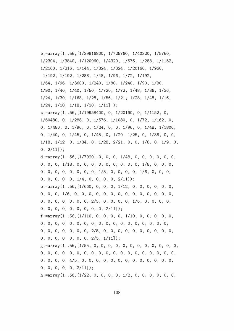
b:=array(1..56,[1/39916800, 1/725760, 1/40320, 1/5760,
1/2304, 1/3840, 1/120960, 1/4320, 1/576, 1/288, 1/1152,
1/2160, 1/216, 1/144, 1/324, 1/324, 1/20160, 1/960,
1/192, 1/192, 1/288, 1/48, 1/96, 1/72, 1/192,
1/64, 1/96, 1/3600, 1/240, 1/80, 1/240, 1/90, 1/30,
1/90, 1/40, 1/40, 1/50, 1/720, 1/72, 1/48, 1/36, 1/36,
1/24, 1/30, 1/168, 1/28, 1/56, 1/21, 1/28, 1/48, 1/16,
1/24, 1/18, 1/18, 1/10, 1/11] );
c:=array(1..56,[1/19958400, 0, 1/20160, 0, 1/1152, 0,
1/60480, 0, 1/288, 0, 1/576, 1/1080, 0, 1/72, 1/162, 0,
0, 1/480, 0, 1/96, 0, 1/24, 0, 0, 1/96, 0, 1/48, 1/1800,
0, 1/40, 0, 1/45, 0, 1/45, 0, 1/20, 1/25, 0, 1/36, 0, 0,
1/18, 1/12, 0, 1/84, 0, 1/28, 2/21, 0, 0, 1/8, 0, 1/9, 0,
0, 2/11]);
d:=array(1..56,[1/7920, 0, 0, 0, 1/48, 0, 0, 0, 0, 0, 0,
0, 0, 0, 1/18, 0, 0, 0, 0, 0, 0, 0, 0, 0, 1/8, 0, 0, 0,
0, 0, 0, 0, 0, 0, 0, 0, 1/5, 0, 0, 0, 0, 1/6, 0, 0, 0,
0, 0, 0, 0, 0, 1/4, 0, 0, 0, 0, 2/11]);
e:=array(1..56,[1/660, 0, 0, 0, 1/12, 0, 0, 0, 0, 0, 0,
0, 0, 0, 1/6, 0, 0, 0, 0, 0, 0, 0, 0, 0, 0, 0, 0, 0, 0,
0, 0, 0, 0, 0, 0, 0, 2/5, 0, 0, 0, 0, 1/6, 0, 0, 0, 0,
0, 0, 0, 0, 0, 0, 0, 0, 0, 2/11]);
f:=array(1..56,[1/110, 0, 0, 0, 0, 1/10, 0, 0, 0, 0, 0,
0, 0, 0, 0, 0, 0, 0, 0, 0, 0, 0, 0, 0, 0, 0, 0, 0, 0,
0, 0, 0, 0, 0, 0, 0, 2/5, 0, 0, 0, 0, 0, 0, 0, 0, 0, 0,
0, 0, 0, 0, 0, 0, 0, 2/5, 1/11]);
g:=array(1..56,[1/55, 0, 0, 0, 0, 0, 0, 0, 0, 0, 0, 0, 0,
0, 0, 0, 0, 0, 0, 0, 0, 0, 0, 0, 0, 0, 0, 0, 0, 0, 0, 0,
0, 0, 0, 0, 4/5, 0, 0, 0, 0, 0, 0, 0, 0, 0, 0, 0, 0, 0,
0, 0, 0, 0, 0, 2/11]);
h:=array(1..56,[1/22, 0, 0, 0, 0, 1/2, 0, 0, 0, 0, 0, 0,
108
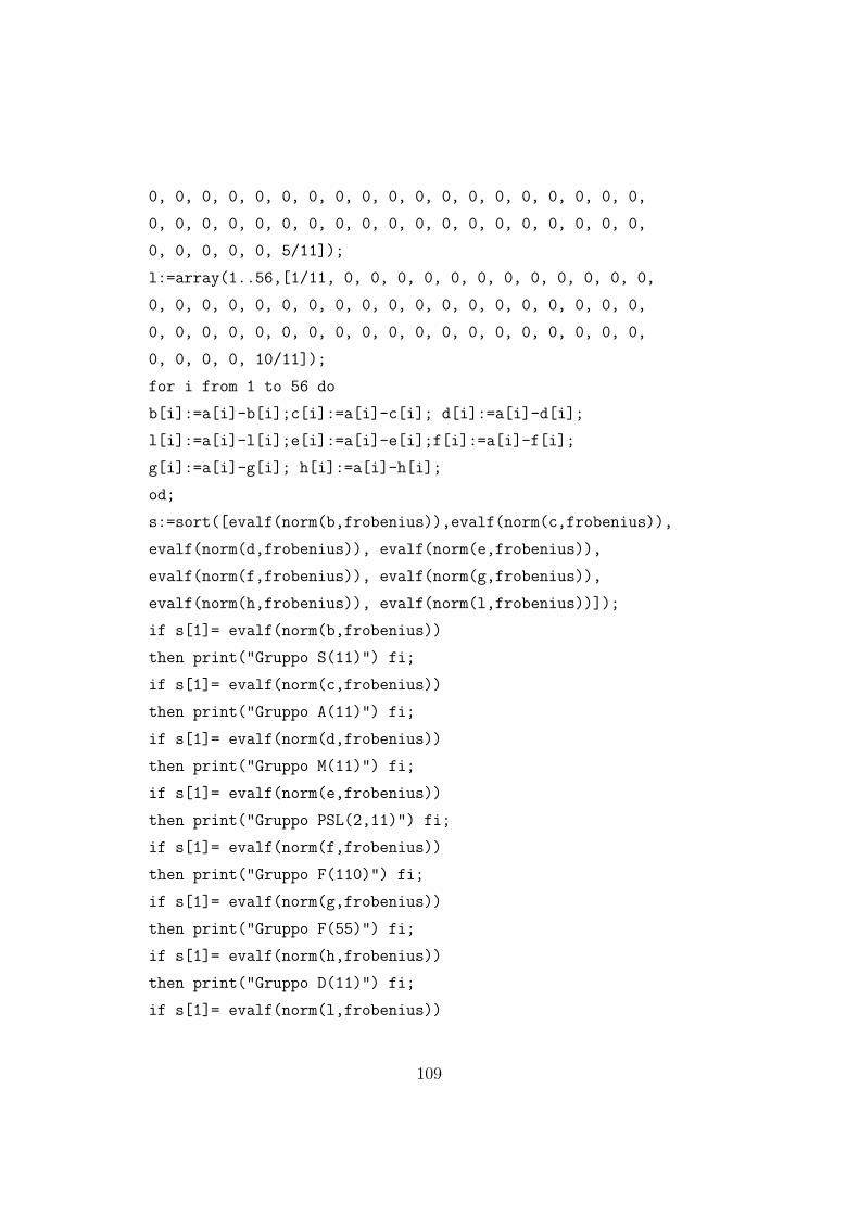
0, 0, 0, 0, 0, 0, 0, 0, 0, 0, 0, 0, 0, 0, 0, 0, 0, 0, 0,
0, 0, 0, 0, 0, 0, 0, 0, 0, 0, 0, 0, 0, 0, 0, 0, 0, 0, 0,
0, 0, 0, 0, 0, 5/11]);
l:=array(1..56,[1/11, 0, 0, 0, 0, 0, 0, 0, 0, 0, 0, 0, 0,
0, 0, 0, 0, 0, 0, 0, 0, 0, 0, 0, 0, 0, 0, 0, 0, 0, 0, 0,
0, 0, 0, 0, 0, 0, 0, 0, 0, 0, 0, 0, 0, 0, 0, 0, 0, 0, 0,
0, 0, 0, 0, 10/11]);
for i from 1 to 56 do
b[i]:=a[i]-b[i];c[i]:=a[i]-c[i]; d[i]:=a[i]-d[i];
l[i]:=a[i]-l[i];e[i]:=a[i]-e[i];f[i]:=a[i]-f[i];
g[i]:=a[i]-g[i]; h[i]:=a[i]-h[i];
od;
s:=sort([evalf(norm(b,frobenius)),evalf(norm(c,frobenius)),
evalf(norm(d,frobenius)), evalf(norm(e,frobenius)),
evalf(norm(f,frobenius)), evalf(norm(g,frobenius)),
evalf(norm(h,frobenius)), evalf(norm(l,frobenius))]);
if s[1]= evalf(norm(b,frobenius))
then print("Gruppo S(11)") fi;
if s[1]= evalf(norm(c,frobenius))
then print("Gruppo A(11)") fi;
if s[1]= evalf(norm(d,frobenius))
then print("Gruppo M(11)") fi;
if s[1]= evalf(norm(e,frobenius))
then print("Gruppo PSL(2,11)") fi;
if s[1]= evalf(norm(f,frobenius))
then print("Gruppo F(110)") fi;
if s[1]= evalf(norm(g,frobenius))
then print("Gruppo F(55)") fi;
if s[1]= evalf(norm(h,frobenius))
then print("Gruppo D(11)") fi;
if s[1]= evalf(norm(l,frobenius))
109
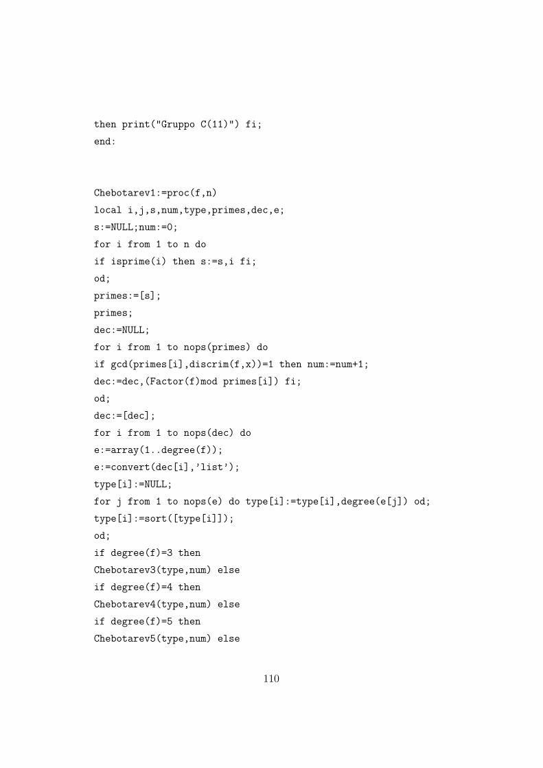
then print("Gruppo C(11)") fi;
end:
Chebotarev1:=proc(f,n)
local i,j,s,num,type,primes,dec,e;
s:=NULL;num:=0;
for i from 1 to n do
if isprime(i) then s:=s,i fi;
od;
primes:=[s];
primes;
dec:=NULL;
for i from 1 to nops(primes) do
if gcd(primes[i],discrim(f,x))=1 then num:=num+1;
dec:=dec,(Factor(f)mod primes[i]) fi;
od;
dec:=[dec];
for i from 1 to nops(dec) do
e:=array(1..degree(f));
e:=convert(dec[i],’list’);
type[i]:=NULL;
for j from 1 to nops(e) do type[i]:=type[i],degree(e[j]) od;
type[i]:=sort([type[i]]);
od;
if degree(f)=3 then
Chebotarev3(type,num) else
if degree(f)=4 then
Chebotarev4(type,num) else
if degree(f)=5 then
Chebotarev5(type,num) else
110

if degree(f)=6 then
Chebotarev6(type,num) else
if degree(f)=7 then
Chebotarev7(type,num) else
if degree(f)=11 then
Chebotarev11(type,num)
fi;fi;fi;fi;fi;fi;
end:
Chebotarev:=proc(f,n)
if irreduc(f) then
Chebotarev1(f,n); print(galois(f)) else
print("Errore: il polinomio e riducibile!") fi;
end:
111
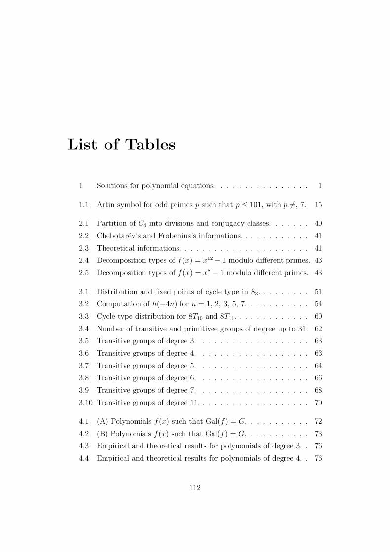
List of Tables
1 Solutions for polynomial equations. . . . . . . . . . . . . . . . 1
1.1 Artin symbol for odd primes p such that p ≤ 101, with p 6=, 7. 15
2.1 Partition of C4 into divisions and conjugacy classes. . . . . . . 40
2.2 Chebotarev’s and Frobenius’s informations. . . . . . . . . . . . 41
2.3 Theoretical informations. . . . . . . . . . . . . . . . . . . . . . 41
2.4 Decomposition types of f(x) = x12 − 1 modulo different primes. 43
2.5 Decomposition types of f(x) = x8 − 1 modulo different primes. 43
3.1 Distribution and fixed points of cycle type in S3. . . . . . . . . 51
3.2 Computation of h(−4n) for n = 1, 2, 3, 5, 7. . . . . . . . . . . 54
3.3 Cycle type distribution for 8T10 and 8T11. . . . . . . . . . . . . 60
3.4 Number of transitive and primitivee groups of degree up to 31. 62
3.5 Transitive groups of degree 3. . . . . . . . . . . . . . . . . . . 63
3.6 Transitive groups of degree 4. . . . . . . . . . . . . . . . . . . 63
3.7 Transitive groups of degree 5. . . . . . . . . . . . . . . . . . . 64
3.8 Transitive groups of degree 6. . . . . . . . . . . . . . . . . . . 66
3.9 Transitive groups of degree 7. . . . . . . . . . . . . . . . . . . 68
3.10 Transitive groups of degree 11. . . . . . . . . . . . . . . . . . . 70
4.1 (A) Polynomials f(x) such that Gal(f) = G. . . . . . . . . . . 72
4.2 (B) Polynomials f(x) such that Gal(f) = G. . . . . . . . . . . 73
4.3 Empirical and theoretical results for polynomials of degree 3. . 76
4.4 Empirical and theoretical results for polynomials of degree 4. . 76
112
4.5 Empirical and theoretical results for polynomials of degree 5. . 77
4.6 Computation of ε(G) for x3 + 2. . . . . . . . . . . . . . . . . . 77
4.7 Computation of ε(G) for x4 + 2. . . . . . . . . . . . . . . . . . 78
4.8 Computation of ε(G) for x5 + 2. . . . . . . . . . . . . . . . . . 78
4.9 Computation of ε(G) for x6 + 2. . . . . . . . . . . . . . . . . . 78
4.10 Computation of ε(G) for x7 + 2. . . . . . . . . . . . . . . . . . 78
4.11 Computation of ε(G) for x11 + 2. . . . . . . . . . . . . . . . . 78
4.12 Comparing ε(G) with respect to k. Degree 3 . . . . . . . . . . 79
4.13 Comparing ε(G) with respect to k. Degree 4 . . . . . . . . . . 79
4.14 Comparing ε(G) with respect to k. Degree 5 . . . . . . . . . . 80
4.15 (A) Comparing ε(G) with respect to k. Degree 6. . . . . . . . 80
4.16 (B) Comparing ε(G) with respect to k. Degree 6 . . . . . . . . 81
4.17 (A) Comparing ε(G) with respect to k. Degree 7. . . . . . . . 81
4.18 (B) Comparing ε(G) with respect to k. Degree 7. . . . . . . . 82
4.19 Comparing ε(G) with respect to k. . . . . . . . . . . . . . . . 82
113

Bibliography
[BM83] Gregory Butler and John McKay. The transitive groups of degree
up to 11. Communications in Algebra, 11:863–911, 1983.
[Bra86] Rolf Brandl. Integer polynomials that are reducible modulo all
primes. Amer. Math. Monthly, 93(4):286–288, 1986.
[Bur55] W. Burnside. Theory of groups of finite order. Dover Publications
Inc., New York, 1955. 2d ed.
[CHM98] John H. Conway, Alexander Hulpke, and John McKay. On transi-
tive permutation groups. j-LMS-J-COMPUT-MATH, 1:1–8, 1998.
[Cox89] David A. Cox. Primes of the form x2 + ny2. A Wiley-Interscience
Publication. John Wiley & Sons Inc., New York, 1989. Fermat,
class field theory and complex multiplication.
[EFM79] D. W. Erbach, J. Fisher, and J. McKay. Polynomials with
PSL(2, 7) as Galois group. J. Number Theory, 11(1):69–75, 1979.
[Jan96] Gerald J. Janusz. Algebraic number fields, volume 7 of Graduate
Studies in Mathematics. American Mathematical Society, Provi-
dence, RI, second edition, 1996.
[Jor72] C. Jordan. Recherches sur les substitutions. Liouville Journal.,
2(17):351–368, 1872.
114
[Lan94] Serge Lang. Algebraic number theory, volume 110 of Graduate
Texts in Mathematics. Springer-Verlag, New York, second edition,
1994.
[LN86] Rudolf Lidl and Harald Niederreiter. Introduction to finite fields
and their applications. Cambridge University Press, Cambridge,
1986.
[LN94] Rudolf Lidl and Harald Niederreiter. Introduction to finite fields
and their applications. Cambridge University Press, Cambridge,
first edition, 1994.
[LO77] J. C. Lagarias and A. M. Odlyzko. Effective versions of the Cheb-
otarev density theorem. In Algebraic number fields: L-functions
and Galois properties (Proc. Sympos., Univ. Durham, Durham,
1975), pages 409–464. Academic Press, London, 1977.
[LS91] H. W. Lenstra, Jr. and P. Stevenhagen. Primes of degree one and
algebraic cases of Cebotarev’s theorem. Enseign. Math. (2), 37(1-
2):17–30, 1991.
[McK79] J. McKay. Some remarks on computing Galois groups. SIAM J.
Comput., 8(3):344–347, 1979.
[MM97] Thomas Mattman and John McKay. Computation of Galois groups
over function fields. Math. Comp., 66(218):823–831, 1997.
[Rot95] Joseph J. Rotman. An introduction to the theory of groups, volume
148 of Graduate Texts in Mathematics. Springer-Verlag, New York,
fourth edition, 1995.
[Saf54] I. R. Safarevic. Construction of fields of algebraic numbers with
given solvable Galois group. Izv. Akad. Nauk SSSR. Ser. Mat.,
18:525–578, 1954.
115

[Sam67] Pierre Samuel. Theorie algebrique des nombres. Hermann, Paris,
1967.
[Ser92] Jean-Pierre Serre. Topics in Galois theory, volume 1 of Research
Notes in Mathematics. Jones and Bartlett Publishers, Boston, MA,
1992. Lecture notes prepared by Henri Damon [Henri Darmon],
With a foreword by Darmon and the author.
[Ser03] Jean-Pierre Serre. On a theorem of Jordan. Bull. Amer. Math.
Soc. (N.S.), 40(4):429–440 (electronic), 2003.
[SL96] P. Stevenhagen and H. W. Lenstra, Jr. Chebotarev and his density
theorem. Math. Intelligencer, 18(2):26–37, 1996.
[SM85] Leonard Soicher and John McKay. Computing Galois groups over
the rationals. J. Number Theory, 20(3):273–281, 1985.
[ST02] Ian Stewart and David Tall. Algebraic number theory and Fermat’s
last theorem. A K Peters Ltd., Natick, MA, third edition, 2002.
[Sta73] Richard P. Stauduhar. The determination of Galois groups. Math.
Comp., 27:981–996, 1973.
[vdW91] B. L. van der Waerden. Algebra. Vol. I. Springer-Verlag, New
York, 1991. Based in part on lectures by E. Artin and E. Noether,
Translated from the seventh German edition by Fred Blum and
John R. Schulenberger.
[Vol96] Helmut Volklein. Groups as Galois groups, volume 53 of Cambridge
Studies in Advanced Mathematics. Cambridge University Press,
Cambridge, 1996. An introduction.
[Wym72] B. F. Wyman. What is a reciprocity law? Amer. Math. Monthly,
79:571–586; correction, ibid. 80 (1973), 281, 1972.
116