the characteristics of surface albedo change trends over

remote sensing

Article

The Characteristics of Surface Albedo ChangeTrends over the Antarctic Sea Ice Regionduring Recent Decades

Chunxia Zhou, Teng Zhang * and Lei Zheng

Chinese Antarctic Center of Surveying and Mapping, Wuhan University, Wuhan 430079, China;[email protected] (C.Z.); [email protected] (L.Z.)* Correspondence: [email protected]

Received: 31 January 2019; Accepted: 3 April 2019; Published: 5 April 2019��

Abstract: Based on a long-time series (1982–2015) of remote sensing data, we analyzed the changein surface albedo (SAL) during summer (from December to the following February) for the entireAntarctic Sea Ice Region (ASIR) and five longitudinal sectors around Antarctica: (1). the Weddell Sea(WS), (2). Indian Ocean, (3). Pacific Ocean (PO), (4). Ross Sea, and (5). Bellingshausen–AmundsenSea (BS). Empirical mode decomposition was used to extract the trend of the original signal, and thena slope test method was utilized to identify a transition point. The SAL provided by the CM SAFcloud, Albedo, and Surface Radiation dataset from AVHRR data-Second Edition was validated atNeumayer station. Sea ice concentration (SIC) and sea surface temperature (SST) were also analyzed.The trend of the SAL/SIC was positive during summer over the ASIR and five longitudinal sectors,except for the BS (−2.926% and −4.596% per decade for SAL and SIC, correspondingly). Moreover,the largest increasing trend of SAL and SIC appeared in the PO at approximately 3.781% and 3.358%per decade, respectively. However, the decreasing trend of SAL/SIC in the BS slowed down, and theincreasing trend of SAL/SIC in the PO accelerated. The trend curves of the SST exhibited a crestaround 2000–2005; thus, the slope lines of the SST showed an increasing–decreasing type for the ASIRand the five longitudinal sectors. The evolution of summer albedo decreased rapidly in the earlysummer and then maintained a relatively stable level for the whole ASIR. The change of it mainlydepended on the early melt of sea ice during the entire summer. The change of sea ice albedo had anarrow range when compared with composite albedo and SIC over the five longitudinal sectors andreached a stable level earlier. The transition point of SAL/SIC in several sectors appeared around theyear 2000, whereas that of the SST for the entire ASIR occurred in 2003–2005. A high value of SAL/SICand a low value of the SST existed in the WS which can be displayed by the spatial distribution ofpixel average. In addition, the lower the latitude was, the lower the SAL/SIC and the higher the SSTwould be. A transition point of SAL appeared in 2001 in most areas of West Antarctica. This transitionpoint could be illustrated by anomaly maps. The spatial distribution of the pixel-based trend ofSAL demonstrated that the change in SAL in East Antarctica has exhibited a positive trend in recentdecades. However, in West Antarctica, the change of SAL presented a decreasing trend before 2001and transformed into an increasing trend afterward, especially in the east of the Antarctic Peninsula.

Keywords: Antarctica; ensemble empirical mode; sea ice albedo; sea ice concentration; sea surfacetemperature

1. Introduction

Antarctica is sensitive to climate change despite its isolation from human beings [1,2]. Interestingly,the Antarctic is also known as an “indicator” of global climate change [3]. One of the deepest warming

Remote Sens. 2019, 11, 821; doi:10.3390/rs11070821 www.mdpi.com/journal/remotesensing

http://www.mdpi.com/journal/remotesensing

http://www.mdpi.com

https://orcid.org/0000-0002-3698-0536

http://www.mdpi.com/2072-4292/11/7/821?type=check_update&version=1

http://dx.doi.org/10.3390/rs11070821

http://www.mdpi.com/journal/remotesensing

Remote Sens. 2019, 11, 821 2 of 25

rates on Earth has been recorded in the Antarctic Peninsula (with an increase of 0.056 ◦C per yearsince 1950) which was reported by Turner et al. (2005) [4]. The recent results of Turner et al. (2016)indicated that this trend has weakened in recent years [5]. However, several works have presentedpreliminary evidence that the warming trend has slowed down since the beginning of the 21st century,and a cooling trend has occurred in the recent two decades [6–9]. The variations in sea ice in Antarcticahave played a key role in climate changes [10–13]. Therefore, to improve our understanding of theclimate change, we must analyze the changes in the Antarctic sea ice in recent decades.

The changes in Antarctic sea ice considerably affect the change in climate over Antarctica [14–17].The increased absorption of sunlight through the earth–atmosphere system results in increasingtemperature and the warming of the ocean, thereby further causing a decrease in the sea ice extent andsurface albedo (SAL). This effect is called ice–albedo feedback [18–20]. The Arctic sea ice is becomingthin and young, whereas the sea ice extent in Antarctica has slightly increased over the last fourdecades [21–23]. Parkinson et al. (2012) used satellite passive–microwave data and found a substantialincreasing trend (17100 ± 2300 km2 year−1) of sea ice extent over Antarctica from 1978 to 2010 [24].Turner et al. (2016) determined an increasing trend by 195 × 103 km2 per decade for the total Antarcticsea ice extent from 1979 to 2013 [25]. However, on the basis of the transition of the Interdecadal PacificOscillation from the positive to the negative phases around the year 2000, Meehl et al. (2016) reportedthat the Antarctic sea ice extent during summer showed a slightly decreasing trend before the 2000sand a considerable increasing trend afterward [7]. De Santis et al. (2017) analyzed the variability andtrend of satellite-derived Antarctic sea ice extent from 1979 to 2016 and discovered an increasing trendof 1.6± 0.4% per decade [21]. Then, the satellite-derived sea ice extent during 1979 to 2015 was studiedby Jena et al. (2018) who declared that the increasing trend of sea ice extent in the Indian Ocean wasabout 2.4 ± 1.2% per decade [9]. Thus, understanding the changes in sea ice in the Antarctic sea iceregion (ASIR) is essential to global climate research.

The albedo, an important factor that affects the radiation balance of the earth–atmosphere system,has frequently been used for research on global climate change [26–28]. Given the high albedo of snowand ice surfaces, most of the solar radiation on the surface of snow and ice in the ASIR are reflectedback to the atmosphere [29–31]. The albedo of unfrozen ocean is between 5% and 20% and is affectedby solar zenith angle. Snow/ice albedo, which is strongly dependent on incident solar irradiance,snow grain size, and soot content, ranges from 50% to 90%, and fresh snow albedo reaches 90% [32].However, substantial incident solar radiation is absorbed by the Antarctic sea ice during summer;thus, the physical state of the snow/ice surface changes rapidly, such that the melting of snow and iceleads to dramatic changes in snow/ice surface albedo [33,34]. A suitable albedo parameterization ofASIR is crucial for the assessment of ice-albedo feedback in Antarctic climate change [35,36]. For ASIR,the composite albedo is estimated using the area fractions and albedos of sea ice and open water.Because the albedo of open water is very small [32], the albedo of sea ice is the key variable of theparameterization of the composite albedo. Therefore, studying the change in albedo is one step inunderstanding the variation of sea ice and recognizing the trend of climate change in Antarctica.

The Antarctic albedo has been extensively studied owing to its important relationship withclimate change. On the basis of SAL data from several Antarctic sites, Pirazzini (2004) indicatedthat the albedo variability is remarkably correlated with snow/ice metamorphism [27]. Brandt et al.(2005) utilized three ship-based field experiments and measured spectral albedos at ultraviolet, visible,and near-infrared wavelengths for open water, grease ice, nilas, young “gray” ice, young gray-whiteice, and first-year ice, with and without snow cover [37]. Data from Advanced Very High-ResolutionRadiometer (AVHRR) Polar Pathfinder (APP) product was used by Laine (2007) to analyze the changesin albedo in the Antarctic ice sheet and sea ice region from 1981 to 2000 [38]. Shao et al. (2015) used adataset consisting of 28 years of homogenized satellite data to calculate the spring–summer albedoof the entire ASIR [39]. Using the Satellite Application Facility on Climate Monitoring (CM SAF) inthe European Organisation for Exploitation of Meteorological Satellite “The CM SAF Cloud, Albedo,

Remote Sens. 2019, 11, 821 3 of 25

and Surface Radiation dataset from AVHRR data”—first edition (CLARA-A1) product, Seo et al. (2016)analyzed the temporal and spatial variabilities of albedo over the Antarctic ice sheet [40,41].

Climate change detection is one of the core issues in climate change research, and it plays a crucialrole in accurately estimating global and regional climate change trends [42]. Conventionally, linearregression [38], least squares [43], moving average [3] and polynomial [44] are used for trend estimationin climate change research and for many studies of sea ice, particularly in the Polar Regions. In fact,climate change presents a complex nonlinear trend, and most long-term variations in many climaticfactors, such as albedo and temperature, show nonlinear and non-stationary complex processes ofchange [45,46]. Therefore, a variety of scales or periodic climate factors changes are hidden due to thelimitation of the conventional methods. To analyze nonlinear and non-stationary data, Huang et al.(1998) proposed a new time series signal processing method: the empirical mode decomposition(EMD), which has strong self-adaptability and local variation characteristics based on the signal [47].The core idea of the EMD is the so called Hilbert-Huang transform, in which any complicated signalcan be decomposed into finite numbers of ‘intrinsic mode functions’ (IMFs) and a residual mode:long-term trend. Compared with conventional methods, it can extract long-term trends of changes inclimate factors more efficiently [48]. Shu et al. (2012) used the EMD method to analyze the change insea ice in Antarctica and found that the rate of increased trend of sea ice has been accelerating in thepast decade [49]. By decomposing the long-term (from February 1947 to January 2011) temperaturedata observed at Faraday/Vernadsky station using EMD, Franzke (2013) demonstrated that most of thetemperature variability occurred on intraannual time scales [50]. By using the EMD method, the cyclicand non-cyclic components of sea level change were separated by Galassi and Spada (2017) [51].Furthermore, the EMD method has been gradually applied in the field of climate change research,and some significant results have been achieved [52–54].

In this study, we aim to analyze the SAL of sea ice in recent decades (1982–2015) and investigateclimate change over the ASIR. Considering the Antarctic polar night phenomenon, we only analyze thechanges in albedo during summer (December to the following February); these changes also containinteresting albedo variations. To study the regional features of climate change over the ASIR, the regionis divided into five longitudinal sectors around Antarctica [37,55]. Empirical mode decomposition(EMD) is applied to the SAL, sea ice concentration (SIC), and sea surface temperature (SST) to extractthe residual component, which represents their change trend. Then, we use a slope-test method toidentify the transition point. After the time series and trend analysis, the transition points of SAL,SIC and SST are estimated, and then the spatial distributions of SAL, SIC and SST are illustrated.Following the introduction, the second section briefly presents the research region and datasets.The methodology is described in Section 3. In Section 4, the SAL is evaluated by comparison with themeasurements at the Neumayer (GVN) station. The analysis results and discussion are displayed inSection 5. The last section provides the conclusions drawn from this study. To increase the readabilityof this paper, all the acronyms used here are listed in Table 1.

Table 1. List of acronyms.

Acronym Full Name

APP-x AVHRR Polar Pathfinder-ExtendedASIR Antarctic Sea Ice RegionAVG Average

AVHRR Advanced Very High Resolution RadiometerBS Bellingshausen–Amundsen Sea

BSRN Baseline Surface Radiation NetworkCDR Climate Data Record

CLARA-A2 The CM SAF cloud, Albedo, and Surface Radiation dataset from AVHRR data-Second EditionCM SAF Climate Monitoring Satellite Application FacilityDMSP Defense Meteorological Satellite ProgramEMD Empirical Mode DecompositionGVN Neumayer

Remote Sens. 2019, 11, 821 4 of 25

Table 1. Cont.

Acronym Full Name

IMFs Intrinsic Mode FunctionsIO Indian Ocean

NOAA National Oceanic and Atmospheric AdministrationNSIDC National Snow and Ice Data Center

PO Pacific OceanRS Ross Sea

SAL Surface AlbedoSIC Sea Ice Concentration

SMMR Scanning Multichannel Microwave RadiometerSSM/I Special Sensor Microwave/ImagerSSMIS Special Sensor Microwave Imager/Sounder

SST Sea Surface TemperatureSW ShortwaveWS Weddell Sea

2. Research Region and Datasets

2.1. Research Region

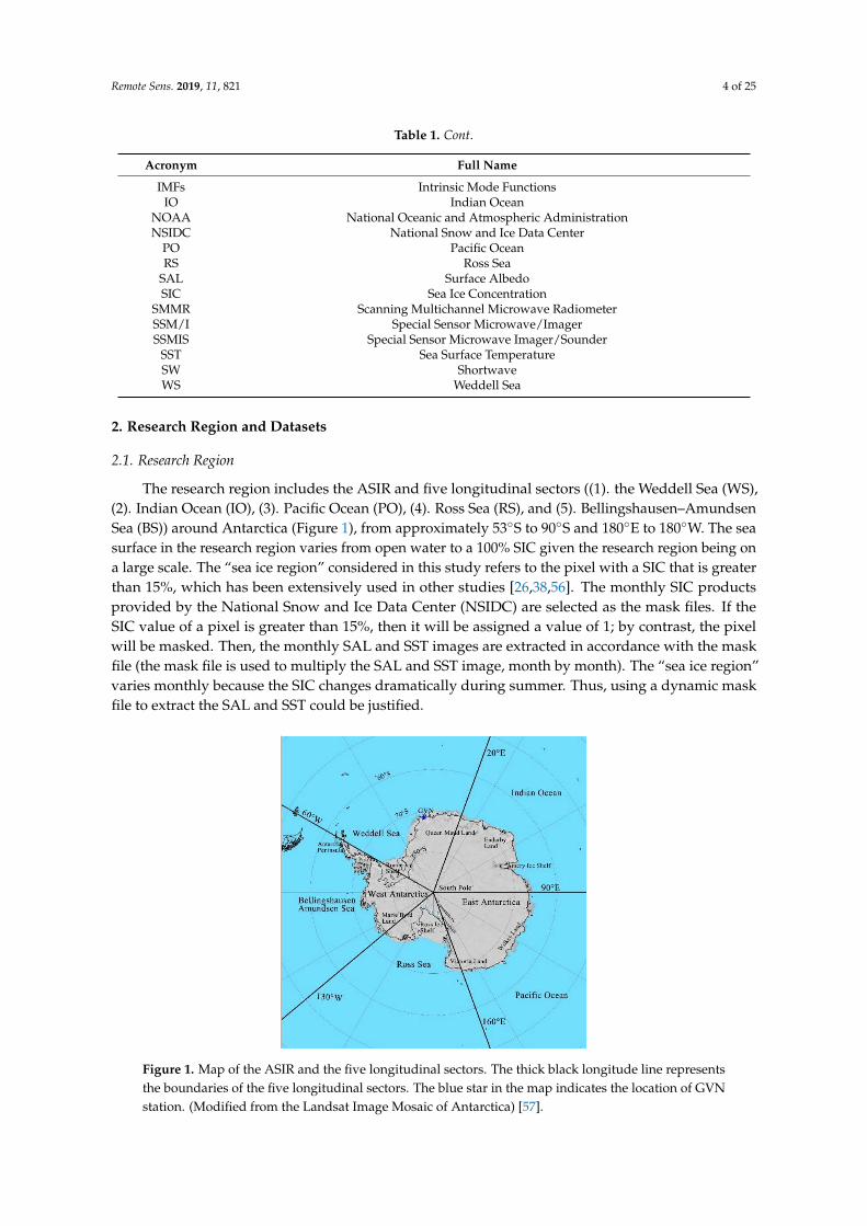
The research region includes the ASIR and five longitudinal sectors ((1). the Weddell Sea (WS),(2). Indian Ocean (IO), (3). Pacific Ocean (PO), (4). Ross Sea (RS), and (5). Bellingshausen–AmundsenSea (BS)) around Antarctica (Figure 1), from approximately 53◦S to 90◦S and 180◦E to 180◦W. The seasurface in the research region varies from open water to a 100% SIC given the research region being ona large scale. The “sea ice region” considered in this study refers to the pixel with a SIC that is greaterthan 15%, which has been extensively used in other studies [26,38,56]. The monthly SIC productsprovided by the National Snow and Ice Data Center (NSIDC) are selected as the mask files. If theSIC value of a pixel is greater than 15%, then it will be assigned a value of 1; by contrast, the pixelwill be masked. Then, the monthly SAL and SST images are extracted in accordance with the maskfile (the mask file is used to multiply the SAL and SST image, month by month). The “sea ice region”varies monthly because the SIC changes dramatically during summer. Thus, using a dynamic maskfile to extract the SAL and SST could be justified.

Remote Sens. 2019, 11, x FOR PEER REVIEW 4 of 25

IO Indian Ocean NOAA National Oceanic and Atmospheric Administration NSIDC National Snow and Ice Data Center

PO Pacific Ocean RS Ross Sea

SAL Surface Albedo SIC Sea Ice Concentration

SMMR Scanning Multichannel Microwave Radiometer SSM/I Special Sensor Microwave/Imager SSMIS Special Sensor Microwave Imager/Sounder

SST Sea Surface Temperature SW Shortwave WS Weddell Sea

2. Research Region and Datasets

2.1. Research Region

The research region includes the ASIR and five longitudinal sectors ((1). the Weddell Sea (WS), (2). Indian Ocean (IO), (3). Pacific Ocean (PO), (4). Ross Sea (RS), and (5). Bellingshausen–Amundsen Sea (BS)) around Antarctica (Figure 1), from approximately 53°S to 90°S and 180°E to 180°W. The sea surface in the research region varies from open water to a 100% SIC given the research region being on a large scale. The “sea ice region” considered in this study refers to the pixel with a SIC that is greater than 15%, which has been extensively used in other studies [26,38,56]. The monthly SIC products provided by the National Snow and Ice Data Center (NSIDC) are selected as the mask files. If the SIC value of a pixel is greater than 15%, then it will be assigned a value of 1; by contrast, the pixel will be masked. Then, the monthly SAL and SST images are extracted in accordance with the mask file (the mask file is used to multiply the SAL and SST image, month by month). The “sea ice region” varies monthly because the SIC changes dramatically during summer. Thus, using a dynamic mask file to extract the SAL and SST could be justified.

Figure 1. Map of the ASIR and the five longitudinal sectors. The thick black longitude line represents the boundaries of the five longitudinal sectors. The blue star in the map indicates the location of GVN station. (Modified from the Landsat Image Mosaic of Antarctica) [57].

Figure 1. Map of the ASIR and the five longitudinal sectors. The thick black longitude line representsthe boundaries of the five longitudinal sectors. The blue star in the map indicates the location of GVNstation. (Modified from the Landsat Image Mosaic of Antarctica) [57].

Remote Sens. 2019, 11, 821 5 of 25

2.2. Datasets

The long-term variations of SAL, SIC and SST were analyzed in this study. The composite albedoof ASIR was provided by the second edition of the satellite–derived climate data record CLARA(“The CM SAF Cloud, Albedo and Surface Radiation dataset from AVHRR data”—second editiondenoted as CLARA-A2). The ice concentration data was obtained from SIC products with a spatialresolution of 25 km provided by NSIDC. The National Oceanic and Atmospheric AdministrationClimate Data Record of the extended APP (APP-x) provided a long-term (1982–present) surfacetemperature. The ground-site dataset was obtained at the GVN station, which was provided by theBaseline Surface Radiation Network (BSRN).

2.2.1. CLARA-A2

The SAL is provided by the second edition of the satellite-derived climate data record calledCLARA-A2 [58,59]. The data record covers a 34-year period from 1982 to 2015. It contains cloud, SALand surface radiation budget products, which are derived from the AVHRR sensor [60]. The mainimprovements of CLARA-A2 are cleaning and homogenizing the basic AVHRR level-1 radiancerecord and systematic use of CALIPSO-CALIOP cloud information for development and validationpurposes. The SAL, which is affected by the inherent optical properties of the surface material andatmosphere, depends on atmosphere effects. It is divided into two kinds, namely, black- and white-skyalbedos. Black-sky albedo can be defined as the ratio of the radiant flux for light reflected by a unitsurface area into the view hemisphere to the illumination radiant flux, when the surface is illuminatedwith a parallel beam of light from a single direction. Whereas white-sky albedo is the ratio of theradiant flux reflected from a unit surface area into the whole hemisphere to the incident radiant flux ofhemispherical angular extent, when the incident radiation is pure diffuse isotropic [61]. The CLARA-A2SAL terrestrial product is a black-sky albedo (wavelength of 0.25–2.5 µm), which is calculated usingcloud mask and AVHRR radiance data. The pentad and monthly mean CLARA-A2 SAL product witha 25 km resolution is used in this study. The CLARA-A2 albedo has been validated against in situalbedo observations from the Baseline Surface Radiation Network, the Greenland Climate Network,and the Tara floating ice camp. Results show a typical accuracy of 3%–15% over snow and ice [62].The composite albedo (α) of each pixel which comprises open water and sea ice can be defined as:

α = Ciαi + Cwαw (1)

where Ci and Cw are the area fractions of sea ice and open water, and αi and αw are their albedos,respectively. Due to the narrow range in the albedo of open water, it can be set to a constant value of7% [63]. The area fractions of sea ice refer to the ice concentration, and only those pixels with an iceconcentration greater than 15% are considered in the calculation of sea ice albedo. The pentad meanCLARA-A2 SAL product has been used to estimate the seasonal variation in sea ice albedo. To matchthe temporal resolution of sea ice albedo, the pentad average of ice concentration is calculated by theaverage of the daily SIC product.

2.2.2. NSIDC

The Scanning Multichannel Microwave Radiometer on the Nimbus-7 satellite of the NationalAeronautics and Space Administration and the Special Sensor Microwave Imager/Sounder sensors onthe Defense Meteorological Satellite Program’s -F8, -F11, -F13, and -F17 provide a long-time series ofthe SIC for investigating the surface characteristics of sea ice covers [11,64–66]. The dataset has beengenerated using the Advanced Microwave Scanning Radiometer-Earth Observing System BootstrapAlgorithm [67]. It is also a key factor in Antarctic climate research and has a significant correlation withthe SAL [68]. The monthly SIC data for the South Polar Region are provided by the NSIDC (BootstrapSea Ice Concentrations from Nimbus-7 SMMR and DMSP SSM/I-SSMIS, Version 3), with a 25 kmspatial resolution. The detailed description of the data and its accuracy can be found in Comiso (2017).

Remote Sens. 2019, 11, 821 6 of 25

2.2.3. APP-x

The variation in surface temperatures can be used to explain the Antarctic climate change [4,69,70].The rise in temperature causes snow/ice melt, thereby resulting in an apparent negative correlationbetween SAL and sea ice surface temperature. The NOAA’s CDR of the extended APP (APP-x) providesa long-time (1982—present) calibrated surface skin temperature data for the Polar Regions [71–73].The APP-x data products are mapped onto a 25-km Equal-Area Scalable Earth-Grid at two local solartimes (i.e., 04:00 and 14:00 for the Arctic and 02:00 and 14:00 for the Antarctic). The detailed descriptionand process of the data can be found in the study of Key et al. (2016) [72]. In this study, the surfaceskin temperature data of the APP-x over the ASIR is used as the SST. The uniformity of illuminationis ensured by adopting only the afternoon data (14:00 LT). However, the data for November andDecember in 1994 and January in 1995 are missing from the archives.

2.2.4. BSRN

The World Climate Research Programme BSRN is established to provide surface radiationmeasurements of high quality and temporal resolution at a limited number of sites worldwide.Such measurements provide typically 1-min averaged shortwave (SW) surface radiation fluxes. Sincethe wavelength range of the CLARA-A2 SAL product is between 0.25–2.5 µm, the downwelling andupwelling SW radiation fluxes can be used to estimate the station albedo (αs), as follows:

αs =SW ↑SW ↓ (2)

where ↓ and ↑ represent the downwelling and upwelling SW radiation fluxes, respectively. The GVNstation is selected to evaluate the SAL products of CLARA-A2 considering that it is located at the edgeof the Antarctic continent. The GVN station (70.65◦S, 8.25◦W) is located on the Ekstrom Ice Shelf inthe northeastern WS. The data is available at the GVN station since 1993. For temporal resolution,the daily and monthly averages are calculated by the average of per minute and day, respectively.

3. Methodology

3.1. EMD

The EMD developed by Huang et al. (1998) was used to analyze the non–linear and non–stationarytime series data [47]. The EMD was the base of the Hilbert–Huang transform, which included aHilbert spectral analysis and an instantaneous frequency computation. After the EMD sifting process,a signal would be decomposed into a finite number of intrinsic mode functions (IMFs) and a residualcomponent, which represents the overall trend of the original signal [44,49,74]. The sifting process wasperformed as follows:

(1) The local maxima and minima are determined in the original time series data.(2) A lower/upper envelope (u1(t)/u2(t)) is estimated by fitting cubic splines to the local minima

(maxima).(3) The difference between the original time series data x(t) and the mean of the envelopes m1(t) as

the first component h1(t) are defined in accordance with the following equations:

m1(t) =u1(t) + u2(t)

2(3)

h1(t) = x(t)−m1(t) (4)

(4) h1(t) is identified as the first IMF c1 if it satisfies the two conditions as follows: (1) throughout thewhole length of a single IMF, the numbers of extrema and zero-crossings must either be equal

Remote Sens. 2019, 11, 821 7 of 25

or differ at most by 1; (2) at any data point, the mean value of the envelope defined by the localmaxima and the envelope defined by the local minima is 0.

(5) If h1(t) does not satisfy one of these conditions, then it is regarded as a new parameter x(t), and thestep in Formulas (1) and (2) is repeated k times until h1k(t) satisfies the conditions or until thedifference between the successive sifted results is smaller than the given limit, which is fixed asσthr = 0.3 in our case.

h1k(t) = h1(k−1)(t)−m1k(t) (5)

σ =N

∑t=0

∣∣∣h1k(t)− h1(k−1)(t)

∣∣∣2h2

1(k−1)(t)

(6)

(6) The first IMF is identified as c1 = h1k, and the residual r1(t) can be obtained by subtracting c1 fromthe original data.

r1(t) = x(t)− c1(t) (7)

(7) Taking the residual r1(t) as the new data, we repeated Steps 1–6 to determine the next IMF.(8) The sifting process is stopped until ri(t) becomes a monotonic function or |ri(t)| is very small.

Finally, the original signal can be written as follows:

x(t) =n

∑i=1

ci(t) + rn(t)

In this study, we defined the residual component rn(t) as the original data trend, which has beenextensively used in different fields.

3.2. Slope Test

After the EMD processing, the residual component (trend curve) of the original signal wasextracted. It was smoother and more stable than the original signal. The trend curve approximateda straight line over a short time interval. Hence, the first order difference method could be used tostudy the features of the change trend of the original signal, such as increases in acceleration anddeceleration, the transition point of trend curve [75,76]. In this study, the slope test method was usedto find the transition point. Its core idea is based on the first order difference method. The method canbe expressed as follows:

(1) A subsample s(t) is selected from the original data y(t), and the lengths of the subsample andoriginal data are denoted as j and k, respectively.

s(l) =j

∑l=1

y(l), j < k (8)

s(l) =j

∑l=1

y(l), j < k (9)

(2) The slope of the subsample used in the linear regression equation is calculated as

slope(

j2+ start_time

)= regress(s(l), timeseries(l)) (10)

where start_time refers to the starting year of the timeseries(l), which corresponds to the subsample;and the function regress is provided by MATLAB R2014b. The function regress is used to estimatethe regression coefficients in the linear model at 95% confidence level.

Remote Sens. 2019, 11, 821 8 of 25

(3) l ∈ (2, j + 1) is set, and Steps 1 and 2 are repeated until l ∈ (k − j + 1, k).(4) Normally, a slope value that is greater/smaller than 0 indicates an increasing/decreasing trend;

in addition, if the sign of the slope transforms from the positive (negative) to the negative(positive) phases, then the trend of the original data has changed and will be defined as thetransition point.

The original data are nonlinear and nonstationary; thus, the slope test fails to process these data.The residual component is smoother and more stable than the original data. Thus, the slope testmethod is adopted to process the residual component to determine the transition point.

4. Validation

The location of the GVN station is shown in Figure 1. Following the evaluation of surface radiationfluxes in Antarctica, the ‘verification area’ refers to the area within 100 km of the GVN station [77,78].The monthly average of the composite albedo is calculated on the basis of the ‘verification area’ andcompared with the data from the GVN site. The statistical parameters contained the mean bias androot mean square error (RMSE).

The average albedo derived from the CLARA-A2 SAL product in summer and the months ofDecember, January and February from 1993 to 2015 were validated with those of the GVN station in thisstudy (Figure 2). As shown in the scatter plot (Figure 2a), the albedo estimated from the CLARA-A2dataset underestimated those in the GVN station during the summer. For each month, the monthlyaverage albedo of CLARA-A2 was also generally lower than those from the GVN site (Figure 2b–d).Hence, the mean biases of summer and each month were less than 0 (Table 2). The mean bias was−2.02% with RMSE of 2.68 during the summer. Moreover, the mean biases and RMSE for each monthwere greater than −2.5% and lower than 4, respectively. In the light of these results, the accuracy ofCLARA-A2 albedo seemed to be consistent with that estimated by Dybbroe et al. (2005) [62].


where start_time refers to the starting year of the timeseries(l), which corresponds to the subsample; and the function regress is provided by MATLAB R2014b. The function regress is used to estimate the regression coefficients in the linear model at 95% confidence level. (3) l(2, j+1) is set, and Steps 1 and 2 are repeated until l(k−j+1, k). (4) Normally, a slope value that is greater/smaller than 0 indicates an increasing/decreasing trend; in addition, if the sign of the slope transforms from the positive (negative) to the negative (positive) phases, then the trend of the original data has changed and will be defined as the transition point.

The original data are nonlinear and nonstationary; thus, the slope test fails to process these data. The residual component is smoother and more stable than the original data. Thus, the slope test method is adopted to process the residual component to determine the transition point.

4. Validation

The location of the GVN station is shown in Figure 1. Following the evaluation of surface radiation fluxes in Antarctica, the ‘verification area’ refers to the area within 100 km of the GVN station [77,78]. The monthly average of the composite albedo is calculated on the basis of the ‘verification area’ and compared with the data from the GVN site. The statistical parameters contained the mean bias and root mean square error (RMSE).

The average albedo derived from the CLARA-A2 SAL product in summer and the months of December, January and February from 1993 to 2015 were validated with those of the GVN station in this study (Figure 2). As shown in the scatter plot (Figure 2a), the albedo estimated from the CLARA-A2 dataset underestimated those in the GVN station during the summer. For each month, the monthly average albedo of CLARA-A2 was also generally lower than those from the GVN site (Figures 2b–d). Hence, the mean biases of summer and each month were less than 0 (Table 2). The mean bias was -2.02% with RMSE of 2.68 during the summer. Moreover, the mean biases and RMSE for each month were greater than -2.5% and lower than 4, respectively. In the light of these results, the accuracy of CLARA-A2 albedo seemed to be consistent with that estimated by Dybbroe et al. (2005) [62].

Figure 2. Comparison of summer and monthly means of albedo observed in Summer (a), December (b), January (c), and February (d) at GVN station with those derived from the CLARA-A2 dataset.

Table 2. Assessment results of albedo (%) between CLARA-A2 dataset and GVN station.

Summer December January February Mean Bias (%) −2.02 −2.17 −1.91 −1.86

RMSE 2.68 2.64 3.15 3.69

Figure 2. Comparison of summer and monthly means of albedo observed in Summer (a), December(b), January (c), and February (d) at GVN station with those derived from the CLARA-A2 dataset.

Table 2. Assessment results of albedo (%) between CLARA-A2 dataset and GVN station.

Summer December January February

Mean Bias (%) −2.02 −2.17 −1.91 −1.86RMSE 2.68 2.64 3.15 3.69

Remote Sens. 2019, 11, 821 9 of 25

5. Results and Discussion

5.1. Long-Term Changes and Trends

The variability and trends of the SAL, SIC and SST were presented in the form of a time seriesof summer averages for 1982–2015. The time series were calculated for the ASIR as a whole andfor the five longitudinal sectors. The SAL, SIC and SST for these sectors were calculated by time-and area-averaging all the values from pixels identified as sea ice for each region. The residualcomponent could present the trend of the original signal; thus, it was used to estimate the slope values.To determine the optimal linear fit for the residual component, the slope values were estimated throughthe least squares method. The statistical significance of each slope value is tested using a standardF-test with a confidence of 95% and 99%. The yearly relationship between these variations is illustratedin Figures 3–5.

The trend of SAL for the ASIR and the five longitudinal sectors exhibited various degrees ofthe increasing trend throughout the time series during summer, except for the BS, which showeda significant decreasing trend (Figure 3). This was generally contrary to that in the Arctic [56].Furthermore, the trend of the BS also showed negative for each month (Figure 3d,f,h), therebyindicating that the climate in the BS presents a warming trend during summer [13,79]. In December,the lowest values of SAL were found in the IO, except for after 2010 (Figure 3c). This was consistentwith the results by Shao et al. (2015) [39]. The SAL in the WS and the RS clearly increased before2002 and slightly decreased after 2002 (Figure 3f), which may have been caused by a negative sealevel pressure which occurred in the early 2000s [80]. However, that in BS showed a decreasing andincreasing trend before and after 2000, correspondingly (Figure 3h). This finding suggested that furtheranalysis of the trend of SAL is required.


5. Results and Discussion

5.1. Long-Term Changes and Trends

The variability and trends of the SAL, SIC and SST were presented in the form of a time series of summer averages for 1982–2015. The time series were calculated for the ASIR as a whole and for the five longitudinal sectors. The SAL, SIC and SST for these sectors were calculated by time- and area-averaging all the values from pixels identified as sea ice for each region. The residual component could present the trend of the original signal; thus, it was used to estimate the slope values. To determine the optimal linear fit for the residual component, the slope values were estimated through the least squares method. The statistical significance of each slope value is tested using a standard F-test with a confidence of 95% and 99%. The yearly relationship between these variations is illustrated in Figures 3–5.

The trend of SAL for the ASIR and the five longitudinal sectors exhibited various degrees of the increasing trend throughout the time series during summer, except for the BS, which showed a significant decreasing trend (Figure 3).This was generally contrary to that in the Arctic [56]. Furthermore, the trend of the BS also showed negative for each month (Figures 3d,f,h), thereby indicating that the climate in the BS presents a warming trend during summer [13,79]. In December, the lowest values of SAL were found in the IO, except for after 2010 (Figure 3c). This was consistent with the results by Shao et al. (2015) [39]. The SAL in the WS and the RS clearly increased before 2002 and slightly decreased after 2002 (Figure 3f), which may have been caused by a negative sea level pressure which occurred in the early 2000s [80]. However, that in BS showed a decreasing and increasing trend before and after 2000, correspondingly (Figure 3h). This finding suggested that further analysis of the trend of SAL is required.

Figure 3. Time series of the averages of SAL (%) during summer (a,b); December (c,d); January (e,f); and February (g,h) provided by the CLARA-A2 dataset for the ASIR and the five longitudinal sectors. The left and right columns represent the original signal and residual components, respectively. The dashed lines in the right column refer to the linear fitting lines.

The slope values of SAL in the BS were negative during summer and for the 3 months (Table 3) due to an anticyclonic circulation trend and equatorward winds in the Bellingshausen Sea enhanced

Figure 3. Time series of the averages of SAL (%) during summer (a,b); December (c,d); January(e,f); and February (g,h) provided by the CLARA-A2 dataset for the ASIR and the five longitudinalsectors. The left and right columns represent the original signal and residual components, respectively.The dashed lines in the right column refer to the linear fitting lines.

Remote Sens. 2019, 11, 821 10 of 25

The slope values of SAL in the BS were negative during summer and for the 3 months (Table 3)due to an anticyclonic circulation trend and equatorward winds in the Bellingshausen Sea enhancedthe heat exchange with lower latitudes [7]. However, those in the ASIR and other sectors were positive,except for those in the RS during February. These results demonstrated that the climate of the ASIRexhibits a cooling trend during summer [24], except for the BS [81]. The trend of the SAL in the RSduring December and January could dominate that of February, thereby causing a positive slope valueduring summer. The steepest positive trend was identified in the PO during summer (3.781% perdecade), largely caused by the trade winds in the Pacific, have significantly strengthened during thepast two decades [82]. This result was consistent with the results of Laine (2007) [38]. The maximumaverages of the SAL existed in the WS (50.38%) during summer, which could be partly explained bythe fact that maximum sea ice extents existed in WS [21].

Table 3. Slope values (% per decade) and averages (%) (AVG) of the SAL during summer and for3 months for the ASIR and the five longitudinal sectors.

RegionSummer December January February

Slope AVG Slope AVG Slope AVG Slope AVG

ASIR 0.851 ** 46.75 0.842 ** 45.42 0.672 ** 44.75 1.387 ** 50.14BS −2.926 ** 48.88 −1.652 ** 49.55 −1.183 ** 47.47 −0.701 ** 49.65WS 0.605 ** 50.38 0.306 * 46.17 0.836 ** 48.38 0.133 ** 56.50IO 1.619 ** 43.37 2.392 ** 38.10 1.527 ** 43.55 1.069 ** 48.46PO 3.781 ** 44.70 2.004 ** 44.82 4.529 ** 43.95 3.780 ** 45.66RS 0.502 ** 42.60 1.120 ** 47.06 1.044 ** 38.94 −0.179 ** 41.98

Note. * and ** indicate statistical significance at the 95% and 99% confidence level, respectively. No * indicates aconfidence level that is lower than 90% using a standard F-test.

Similar to the trend of the SAL, that of the SIC showed an evidently increasing trend during thesummer, except for the BS (Figure 4b), as estimated by Holland (2014) and Hobbs et al. (2016) [55,83],thus illustrating a significant positive correlation between the SAL and the SIC. This can be explainedby the slowdown of the global warming trend and a deepening of the Amundsen Sea Low nearAntarctica [25,84]. In contrast to the change of SIC in the BS, that in the PO presented an increasing trend(Figure 4d,f,h), and the fastest increasing trend was observed in January when the Southern AnnularMode had positive results in more and stronger cyclones [85]. Interestingly, the decreasing/increasingtrend of the SIC in the BS/PO became relatively flat after 2000 (Figure 4h), this may be caused bythe fact that the temperature has remained flat for the past 15 years [84]. However, the trend ofthe SIC showed a crest/trough for the RS/IO around 2000 (increasing/decreasing before 2000 anddecreasing/increasing after 2000) (Figure 4d). This finding indicated that a transition point of climatechange may have existed in the RS/IO around the year 2000.

Consistent with the trend of SAL, the slope values of SIC were mostly positive, except for theBS (Table 4) [25], which further demonstrated that the climate of the ASIR exhibits a cooling trendin recent decades. The steepest increasing trend could be observed in the PO during the summerand each month [7], and the largest slope values were determined in January (5.968% per decade).Clearly, the increasing rate of sea ice was slower in West Antarctica (WS, BS, and RS) than in EastAntarctica (IO and PO), which is consistent with the changes in the surface net radiation reported byZhang et al. (2019) [78]. This result was due to the more severe climate change in West Antarctica thanin East Antarctica [4,86]. The average of the SIC in the WS was highest during the summer and the3 months considering substantial multiyear sea ice [87]; however, simultaneously, that in the IO wasthe lowest largely because of substantial solar radiation absorbed by the East Antarctica sea ice due tothe low solar zenith angle [88,89].

Remote Sens. 2019, 11, 821 11 of 25Remote Sens. 2019, 11, x FOR PEER REVIEW 11 of 25

Figure 4. The same as Figure 3 but for SIC (%).

Consistent with the trend of SAL, the slope values of SIC were mostly positive, except for the BS (Table 4) [25], which further demonstrated that the climate of the ASIR exhibits a cooling trend in recent decades. The steepest increasing trend could be observed in the PO during the summer and each month [7], and the largest slope values were determined in January (5.968% per decade). Clearly, the increasing rate of sea ice was slower in West Antarctica (WS, BS, and RS) than in East Antarctica (IO and PO), which is consistent with the changes in the surface net radiation reported by Zhang et al. (2019) [78]. This result was due to the more severe climate change in West Antarctica than in East Antarctica [4,86]. The average of the SIC in the WS was highest during the summer and the 3 months considering substantial multiyear sea ice [87]; however, simultaneously, that in the IO was the lowest largely because of substantial solar radiation absorbed by the East Antarctica sea ice due to the low solar zenith angle [88,89].

Table 4. As in Table 2 but for SIC. The units of slope and AVG are ‘% per year’ and ‘%’, respectively.

Region Summer December January February


ASIR 0.721** 65.39 0.065** 65.76 0.169 63.75 0.881** 66.60

BS −4.596** 66.05 −2.480** 70.28 −4.354** 66.25 −2.911** 61.49

WS 0.924** 70.99 0.851** 66.92 1.076** 68.70 0.759** 77.20

IO 1.804** 57.47 0.171 54.10 1.176** 60.88 −0.029 57.22

PO 3.358** 65.40 1.176** 65.47 5.968** 67.62 4.347** 63.23

RS 0.971** 59.25 0.447* 68.82 0.779** 54.61 −1.350** 54.36 Note. * and ** indicate statistical significance at the 95% and 99% confidence levels, respectively. No *denotes a confidence level that is lower than 90% using a standard F-test.

The change in SST in the ASIR and the five longitudinal sectors presented a significant increasing trend during the summer and the 3 months (Figure 5). This change was largely caused by the low

Figure 4. The same as Figure 3 but for SIC (%).

Table 4. As in Table 2 but for SIC. The units of slope and AVG are ‘% per year’ and ‘%’, respectively.



ASIR 0.721 ** 65.39 0.065 ** 65.76 0.169 63.75 0.881 ** 66.60BS −4.596 ** 66.05 −2.480 ** 70.28 −4.354 ** 66.25 −2.911 ** 61.49WS 0.924 ** 70.99 0.851 ** 66.92 1.076 ** 68.70 0.759 ** 77.20IO 1.804 ** 57.47 0.171 54.10 1.176 ** 60.88 −0.029 57.22PO 3.358 ** 65.40 1.176 ** 65.47 5.968 ** 67.62 4.347 ** 63.23RS 0.971 ** 59.25 0.447 * 68.82 0.779 ** 54.61 −1.350 ** 54.36

Note. * and ** indicate statistical significance at the 95% and 99% confidence levels, respectively. No * denotes aconfidence level that is lower than 90% using a standard F-test.

The change in SST in the ASIR and the five longitudinal sectors presented a significant increasingtrend during the summer and the 3 months (Figure 5). This change was largely caused by the low SSTvalues before 1988. Notably, the time series curves of the SST in the ASIR and the five longitudinalsectors had considerable peak values near 2002/2003 (Figure 5a,c,e,g); moreover, a crest appearedbetween 2000 and 2005 for the trend curves of the SST (Figure 5b,d,f,h); this may be caused by theInterdecadal Pacific Oscillation which transitioned from positive to negative in the late 1990s [7].This result indicated that a climate transition point exists around the year 2000; this change was similarto that of SAL/SIC. Although the solar zenith angles were lowest in the ASIR during summer [27,90],its SST was below 0 ◦C.

Remote Sens. 2019, 11, 821 12 of 25


SST values before 1988. Notably, the time series curves of the SST in the ASIR and the five longitudinal sectors had considerable peak values near 2002/2003 (Figures 5a,c,e,g); moreover, a crest appeared between 2000 and 2005 for the trend curves of the SST (Figures 5b,d,f,h); this may be caused by the Interdecadal Pacific Oscillation which transitioned from positive to negative in the late 1990s [7]. This result indicated that a climate transition point exists around the year 2000; this change was similar to that of SAL/SIC. Although the solar zenith angles were lowest in the ASIR during summer [27,90], its SST was below 0 °C.

Figure 5. The same as Figure 3 but for SST (°C).

The low SST values in the ASIR and the five longitudinal sectors before 1988 would dominate given the evident increasing trend of temperature, and it seems to be a noisy signal due to the AVHRR-7/9 which had some serious calibration issues; therefore, the slope values (°C per decade) and the average of the SST during the summer and the 3 months for the ASIR and the five longitudinal sectors in 1988–2015 were calculated (Table 5). The trends of SST were nearly positive (with a 99% confidence level) despite the low values of temperature before 1988 were removed; these were similar to the results indicated by Shu et al. (2012) [49]. This result illustrated that the long-term slope values of temperature may conceal the short-term features of climate change. The slope values of the SST were greater in East Antarctica than in West Antarctica during summer and the 3 months because East Antarctica was basically under an ice-free state during the summer [66]. Thus, the average of the SST was also higher in East Antarctica than in West Antarctica [39]. The average of the SST for February was the lowest in the 3 months due to the fact that the end of summer is February in Antarctica.

Table 5. As in Table 2, but for SST. The units of slope and AVG are ‘°C per decade’ and ‘°C’, respectively.



ASIR 0.392** −2.44 0.350** −1.49 0.365** −1.44 0.175** −4.44

Figure 5. The same as Figure 3 but for SST (◦C).

The low SST values in the ASIR and the five longitudinal sectors before 1988 would dominategiven the evident increasing trend of temperature, and it seems to be a noisy signal due to theAVHRR-7/9 which had some serious calibration issues; therefore, the slope values (◦C per decade)and the average of the SST during the summer and the 3 months for the ASIR and the five longitudinalsectors in 1988–2015 were calculated (Table 5). The trends of SST were nearly positive (with a 99%confidence level) despite the low values of temperature before 1988 were removed; these were similarto the results indicated by Shu et al. (2012) [49]. This result illustrated that the long-term slope valuesof temperature may conceal the short-term features of climate change. The slope values of the SSTwere greater in East Antarctica than in West Antarctica during summer and the 3 months because EastAntarctica was basically under an ice-free state during the summer [66]. Thus, the average of the SSTwas also higher in East Antarctica than in West Antarctica [39]. The average of the SST for Februarywas the lowest in the 3 months due to the fact that the end of summer is February in Antarctica.

Table 5. As in Table 2, but for SST. The units of slope and AVG are ‘◦C per decade’ and ‘◦C’, respectively.



ASIR 0.392 ** −2.44 0.350 ** −1.49 0.365 ** −1.44 0.175 ** −4.44BS 0.473 ** −2.30 0.348 ** −1.55 0.404 ** −1.40 0.599 ** −3.99WS 0.300 ** −2.78 0.337 ** −1.53 0.083 −1.60 0.094 ** −5.23IO 0.840 ** −1.81 0.739 ** −1.12 0.951 ** −1.03 0.608 ** −3.45PO 0.568 ** −1.89 0.622 ** −1.40 0.467 ** −1.06 0.343 ** −3.30RS 0.103 −2.50 0.354 ** −1.65 0.292 ** −1.50 0.052 ** −4.34

Note. * and ** indicate statistical significance at the 95% and 99% confidence level, respectively. No * denotes aconfidence level that is lower than 90% using a standard F-test.

Remote Sens. 2019, 11, 821 13 of 25

5.2. Seasonal Evolution of Composite Albedo, SIC and Sea Ice Albedo

To study the changes in composite albedo, SIC and sea ice albedo during summer, their seasonalevolution were presented in the form of 5-day averages from 1 November to 28 February over1982–2015 (Figure 6). Table 6 presents the relationships of composite albedo and SIC or sea ice albedo.For the ASIR, the changes in composite albedo, SIC and sea ice albedo showed a decreasing trendthroughout the time series during summer, and the relationship between composite albedo and SIC(0.992, above 99% confidence level) or sea ice albedo (0.980, above 99% confidence level) exhibited astrong correlation. This finding could be explained by the substantial incident solar irradiance absorbedby the ice-ocean system due to the low solar zenith angles during summer [78]. The decreasing processduring the entire summer could be divided into two phases. The first phase lasted until late December,wherein the composite albedo and SIC presented a rapidly decreasing trend, from 60% and 85% to 45%and 70% for composite albedo and SIC, respectively. However, that of sea ice albedo was distinctlyslow, from 70% to 60%, which may be caused by the convergent winds in early summer, therebydriving the ice edge retreat poleward and activating the ice-albedo feedback [91]. The decreasing trendwas relatively slow after late December, largely due to the negative sea level pressure anomalies thatoccurred around Antarctica during late summer [55]. Therefore, the evolution of composite albedo,SIC and sea ice albedo depended mainly on the early melting of sea ice during summer.

The evolution of composite albedo closely followed the change in SIC (with a strong correlationcoefficient (0.99) at 99% confidence level). Thus, a rapid decrease in composite albedo was observedbefore mid-January over RS (from 60% to 37%), and a stable level (35%) was maintained subsequently.These findings could be partly explained by the presence of deep cyclones, which would efficientlybreak up and export the sea ice equatorward [85]. However, after a slightly decease beforemid-December, the sea ice albedo maintained a relatively stable level (60%) and reached a stablelevel earlier, at approximately one month before composite albedo, which was similar to that in theArctic reported by Lei et al. (2016). Consistent with other studies [14,21,92], the composite albedo andSIC in BS presented a steady decreasing trend during the entire summer. However, the decreasingtrend of sea ice albedo was evidently slower than that of composite albedo and SIC. Interestingly,the time series plots of composite albedo, SIC and sea ice albedo showed a significant trough by theend of December in WS. This phenomenon may be due to the predominantly westerly wind trendsover most of the Southern Ocean during summer and enhanced equatorward winds that existed inmid-summer over WS, thereby increasing the sea ice [80].

The sea ice extent in East Antarctica was relatively lower than that in West Antarctica and wasaccompanied by complex change in wind field and dramatic melt during summer [16,93]. The changesin sea ice in the IO and PO did not show a monotonic downward trend. After a rapid decline beforemid-December, the sea ice in the IO maintained a short increasing process (approximately half amonth). From then onward, a gradually decreasing trend was observed. The evolution characteristicsof sea ice in the PO were similar to those in the IO, but had a slow change trend and long risingprocess (approximately one and a half months). This phenomenon was mainly caused by the changein sea-level pressure in East Antarctica which was stable and the enhanced westerly winds that wouldtransport sea ice from the IO to the PO during summer [7]. The relationships between compositealbedo and SIC were 0.975 and 0.957 in the IO and PO (with a 99% confidence level), respectively.However, the correlation between composite albedo and sea ice albedo were both below 0.9 (with a99% confidence level) in the two regions, indicating that the evolution of composite albedo duringsummer depends more strongly on the change in SIC than on the variation in sea ice albedo.

Remote Sens. 2019, 11, 821 14 of 25


0.9 (with a 99% confidence level) in the two regions, indicating that the evolution of composite albedo during summer depends more strongly on the change in SIC than on the variation in sea ice albedo.

Figure 6. Seasonal evolutions of SIC (%), composite albedo (%) and sea ice albedo (%) within the ASIR and five longitudinal sectors from 1 November to 28 February averaged over 1982–2015.

Table 6. Correlation coefficients between composite albedo and SIC or sea ice albedo for ASIR and five longitudinal sectors.

ASIR RS BS WS IO PO SIC 0.992 0.990 0.955 0.913 0.975 0.957

Sea Ice Albedo 0.980 0.738 0.779 0.809 0.761 0.874

Note: The statistical significance of all correlation coefficients are at 99% confidence level.

5.3. Transition Points of the SAL, SIC, and SST According to the abovementioned time series and trend analysis, a climate transition point

existed in the entire ASIR around 2000–2005. Moreover, for the SAL, SIC and SST, the slope values of the long_time series would obscure the short-term characteristics of climate change. Therefore, the slope test method was used to estimate the residual components of the SAL, SIC and SST to determine the transition point. The time series curves of the residual component were smooth; thus, the length of the subsample was defined as 5 years. If the slope line had passed through the zero line, then a transition point would exist at that moment. For a detailed analysis of the SAL, SIC and SST variation trends during summer and the 3 months for the ASIR and the five longitudinal sectors, we performed a morphological analysis of the residual component and found that morphological variations can be broadly divided into four categories, namely, increasing, increasing–decreasing, decreasing–increasing, and decreasing types.

The time series of the slope values of the SAL during summer and the 3 months are plotted in Figure 7. The transition point of the SAL only existed in the WS during summer, and the increasing/decreasing trend of the SAL exhibited deceleration in the IO/BS (Figure 7a), similar to those observed in the Antarctic ice sheet [41]. The SAL of the ASIR presented a slightly upward trend despite the fact that in the BS decreased rapidly, this was opposite to that in the Arctic sea ice zone [56]. For each month, the slope lines of the IO and the PO were constantly greater than the zero line

Figure 6. Seasonal evolutions of SIC (%), composite albedo (%) and sea ice albedo (%) within the ASIRand five longitudinal sectors from 1 November to 28 February averaged over 1982–2015.

Table 6. Correlation coefficients between composite albedo and SIC or sea ice albedo for ASIR and fivelongitudinal sectors.

ASIR RS BS WS IO PO

SIC 0.992 0.990 0.955 0.913 0.975 0.957Sea Ice Albedo 0.980 0.738 0.779 0.809 0.761 0.874

Note: The statistical significance of all correlation coefficients are at 99% confidence level.

5.3. Transition Points of the SAL, SIC, and SST

According to the abovementioned time series and trend analysis, a climate transition point existedin the entire ASIR around 2000–2005. Moreover, for the SAL, SIC and SST, the slope values of thelong_time series would obscure the short-term characteristics of climate change. Therefore, the slopetest method was used to estimate the residual components of the SAL, SIC and SST to determine thetransition point. The time series curves of the residual component were smooth; thus, the length of thesubsample was defined as 5 years. If the slope line had passed through the zero line, then a transitionpoint would exist at that moment. For a detailed analysis of the SAL, SIC and SST variation trendsduring summer and the 3 months for the ASIR and the five longitudinal sectors, we performed amorphological analysis of the residual component and found that morphological variations can bebroadly divided into four categories, namely, increasing, increasing–decreasing, decreasing–increasing,and decreasing types.

The time series of the slope values of the SAL during summer and the 3 months are plottedin Figure 7. The transition point of the SAL only existed in the WS during summer, and theincreasing/decreasing trend of the SAL exhibited deceleration in the IO/BS (Figure 7a), similarto those observed in the Antarctic ice sheet [41]. The SAL of the ASIR presented a slightly upwardtrend despite the fact that in the BS decreased rapidly, this was opposite to that in the Arctic sea icezone [56]. For each month, the slope lines of the IO and the PO were constantly greater than the zero

Remote Sens. 2019, 11, 821 15 of 25

line (Figure 7b–d), which were located in East Antarctica. The change trend types and transition pointof the SAL are presented in Table 7. The decreasing–increasing type existed in December and February,and the increasing–decreasing type appeared in January. The transition point in West Antarcticaoccurred in February 2000 which is consistent with the climate change on the Antarctic Peninsula [94].


(Figures 7b–d), which were located in East Antarctica. The change trend types and transition point of the SAL are presented in Table 7. The decreasing–increasing type existed in December and February, and the increasing–decreasing type appeared in January. The transition point in West Antarctica occurred in February 2000 which is consistent with the climate change on the Antarctic Peninsula [94].

Figure 7. Slope values of the SAL (% per year) during summer (a), December (b), January (c), and February (d) are estimated through a 5-year slope test method; the ordinate presents the slope value. The black dotted lines represent the horizontal zero line.

Table 7. Change trend types and transition points of the SAL for the ASIR and the five longitudinal sectors during the summer and the 3 months.


Type Point Type Point Type Point Type Point

ASIR ↑ / ↓–↑ 1987 ↑–↓ 2009 ↑ /

BS ↓ / ↓–↑ 2008 ↓ / ↓–↑ 2001

WS ↓–↑ 1992 ↓–↑ 1996 ↑–↓ 2004 ↓–↑ 1996

IO ↑ / ↑ / ↑ / ↑ /

PO ↑ / ↑ / ↑ / ↑ /

RS ↑ / ↑ / ↑–↓ 2003 ↓–↑ 2000 Note. ↑ , ↑–↓ , ↓–↑ , and ↓ represent the four categories, namely, increasing, increasing–decreasing, decreasing–increasing, and decreasing types, respectively.

Although the slope values of the SIC were approximately greater than 0, except for the BS during summer (Figure 8a) [24], the time series of the slope lines for different regions showed different features. For example, the increasing trend in the PO and the RS exhibited acceleration and deceleration, correspondingly [21,24,95], whereas the slope values of the SIC in the IO were essentially constant. The slope lines of the PO and the BS were above and below the zero line during the 3 months (Figures 8b–d), respectively; these slope lines were similar to the SAL. However, the features of the slope lines for the different months were complex and changeable over other regions. This result was largely due to the dramatic climate change during the ASIR summer [13,44]. The transition points of the SIC in the ASIR appeared in December 2001 and January 1999 because that in the five longitudinal sectors appeared around the year 2000, except for the BS and PO.

Figure 7. Slope values of the SAL (% per year) during summer (a), December (b), January (c),and February (d) are estimated through a 5-year slope test method; the ordinate presents the slopevalue. The black dotted lines represent the horizontal zero line.

Table 7. Change trend types and transition points of the SAL for the ASIR and the five longitudinalsectors during the summer and the 3 months.



ASIR ↑ / ↓–↑ 1987 ↑–↓ 2009 ↑ /BS ↓ / ↓–↑ 2008 ↓ / ↓–↑ 2001WS ↓–↑ 1992 ↓–↑ 1996 ↑–↓ 2004 ↓–↑ 1996IO ↑ / ↑ / ↑ / ↑ /PO ↑ / ↑ / ↑ / ↑ /RS ↑ / ↑ / ↑–↓ 2003 ↓–↑ 2000

Note. ↑, ↑–↓, ↓–↑, and ↓ represent the four categories, namely, increasing, increasing–decreasing,decreasing–increasing, and decreasing types, respectively.

Although the slope values of the SIC were approximately greater than 0, except for the BSduring summer (Figure 8a) [24], the time series of the slope lines for different regions showed differentfeatures. For example, the increasing trend in the PO and the RS exhibited acceleration and deceleration,correspondingly [21,24,95], whereas the slope values of the SIC in the IO were essentially constant.The slope lines of the PO and the BS were above and below the zero line during the 3 months(Figure 8b–d), respectively; these slope lines were similar to the SAL. However, the features of theslope lines for the different months were complex and changeable over other regions. This result waslargely due to the dramatic climate change during the ASIR summer [13,44]. The transition points ofthe SIC in the ASIR appeared in December 2001 and January 1999 because that in the five longitudinalsectors appeared around the year 2000, except for the BS and PO (Table 8).


Figure 8. The same as Figure 7 but for SIC (% per year).

Table 8. As in Table 5 but for SIC.



ASIR ↑ / ↑–↓ 2001 ↑–↓ 1999 ↑ /

BS ↓ / ↓ / ↓ / ↓ /

WS ↓–↑ 1986 ↓–↑ 1995 ↑–↓ 2002 ↑ /

IO ↑ / ↓–↑ 1997 ↓–↑ 1986 ↓–↑ 2000

PO ↑ / ↑–↓ 2009 ↑ / ↑ /

RS ↑ / ↑–↓ 2000 ↑–↓ 2001 ↓ / Note. ↑, ↑–↓, ↓–↑, and ↓ correspond to the four categories, namely, increasing, increasing–decreasing, decreasing–increasing, and decreasing types.

The slope lines of the SST for the ASIR and the five longitudinal sectors were positive before 2000–2005 and negative afterward (Figure 9a). This result demonstrated that a cooling trend of climate occurs in the whole ASIR in 2000–2005 [80]. During summer, the slowest increasing trend of the SST appeared in the PO before 2000 [96,97]. Although the slope lines were above the zero line in February (Figure 9d), the warming trend in the IO and the PO presented acceleration and deceleration, respectively. In contrast to the characteristics of the slope lines of SAL/SIC, the morphological type of the SST in the ASIR and the five longitudinal sectors during summer and the 3 months was increasing–decreasing, except for that in the PO and IO in February (Table 9). Furthermore, the transition points of the ASIR and the five longitudinal sectors were around 2003–2005 and are generally in step with global surface temperature change [98].

Figure 8. The same as Figure 7 but for SIC (% per year).

Table 8. As in Table 5 but for SIC.



ASIR ↑ / ↑–↓ 2001 ↑–↓ 1999 ↑ /BS ↓ / ↓ / ↓ / ↓ /WS ↓–↑ 1986 ↓–↑ 1995 ↑–↓ 2002 ↑ /IO ↑ / ↓–↑ 1997 ↓–↑ 1986 ↓–↑ 2000PO ↑ / ↑–↓ 2009 ↑ / ↑ /RS ↑ / ↑–↓ 2000 ↑–↓ 2001 ↓ /

Note. ↑, ↑–↓, ↓–↑, and ↓ correspond to the four categories, namely, increasing, increasing–decreasing,decreasing–increasing, and decreasing types.

The slope lines of the SST for the ASIR and the five longitudinal sectors were positive before2000–2005 and negative afterward (Figure 9a). This result demonstrated that a cooling trend of climateoccurs in the whole ASIR in 2000–2005 [80]. During summer, the slowest increasing trend of theSST appeared in the PO before 2000 [96,97]. Although the slope lines were above the zero line inFebruary (Figure 9d), the warming trend in the IO and the PO presented acceleration and deceleration,respectively. In contrast to the characteristics of the slope lines of SAL/SIC, the morphologicaltype of the SST in the ASIR and the five longitudinal sectors during summer and the 3 monthswas increasing–decreasing, except for that in the PO and IO in February (Table 9). Furthermore,the transition points of the ASIR and the five longitudinal sectors were around 2003–2005 and aregenerally in step with global surface temperature change [98].

Table 9. As in Table 5 but for SST.



ASIR ↑–↓ 2003 ↑–↓ 2003 ↑–↓ 2003 ↑–↓ 2003BS ↑–↓ 2003 ↑–↓ 2004 ↑–↓ 2004 ↑–↓ 2006WS ↑–↓ 2003 ↑–↓ 2004 ↑–↓ 2002 ↑–↓ 2003IO ↑–↓ 2005 ↑–↓ 2004 ↑–↓ 2005 ↑ /PO ↑–↓ 2004 ↑–↓ 2006 ↑–↓ 2004 ↑ /RS ↑–↓ 2001 ↑–↓ 2006 ↑–↓ 2003 ↑–↓ 2003

Note. ↑, ↑–↓, ↓–↑, and ↓ represent the four categories, namely, increasing, increasing–decreasing,decreasing–increasing, and decreasing types, respectively.


Figure 9. The same as Figure 7 but for SST (°C per year).

Table 9. As in Table 5 but for SST.



ASIR ↑–↓ 2003 ↑–↓ 2003 ↑–↓ 2003 ↑–↓ 2003

BS ↑–↓ 2003 ↑–↓ 2004 ↑–↓ 2004 ↑–↓ 2006

WS ↑–↓ 2003 ↑–↓ 2004 ↑–↓ 2002 ↑–↓ 2003

IO ↑–↓ 2005 ↑–↓ 2004 ↑–↓ 2005 ↑ /

PO ↑–↓ 2004 ↑–↓ 2006 ↑–↓ 2004 ↑ /

RS ↑–↓ 2001 ↑–↓ 2006 ↑–↓ 2003 ↑–↓ 2003 Note. ↑ , ↑–↓ , ↓–↑ , and ↓ represent the four categories, namely, increasing, increasing–decreasing, decreasing–increasing, and decreasing types, respectively.

5.4. Spatial Distribution

To illustrate the average spatial distributions of the SAL, SIC and SST, the maps were prepared for the average summer SAL, SIC and SST of the whole ASIR for the entire 33 years (Figure 10).

Because positive sea-level pressure anomalies and northward winds appeared in the Southern Atlantic Ocean [7], the SIC in the WS was high during summer (Figure 10b); thus, the high SAL could also be found in the WS (Figure 10a) [37,83]. Moreover, the low values of the SST existed in the WS (Figure 10c), thereby indicating that the spatial correlation between the SAL and the SIC was significantly positive, and that between SAL/SIC and SST was negative [99]. The low pixel average of SAL/SIC and high pixel average of the SST appeared on the edge of the sea ice, which was largely due to the solar radiation that was absorbed when the latitude was low [31], and positive (negative) cyclone density anomalies emerged around Antarctica (mid-latitudes) [85]. Minimal sea ice existed in East Antarctica; thus, the SAL and SIC were evidently smaller in East Antarctica than in West Antarctica. The average SAL (Table 3), SIC (Table 4), and SST (Table 5) for the total ASIR were 46.75%, 65.39%, and −2.44 °C during summer.

Figure 9. The same as Figure 7 but for SST (◦C per year).

5.4. Spatial Distribution

To illustrate the average spatial distributions of the SAL, SIC and SST, the maps were preparedfor the average summer SAL, SIC and SST of the whole ASIR for the entire 33 years (Figure 10).

Because positive sea-level pressure anomalies and northward winds appeared in the SouthernAtlantic Ocean [7], the SIC in the WS was high during summer (Figure 10b); thus, the high SALcould also be found in the WS (Figure 10a) [37,83]. Moreover, the low values of the SST existed inthe WS (Figure 10c), thereby indicating that the spatial correlation between the SAL and the SIC wassignificantly positive, and that between SAL/SIC and SST was negative [99]. The low pixel average ofSAL/SIC and high pixel average of the SST appeared on the edge of the sea ice, which was largely dueto the solar radiation that was absorbed when the latitude was low [31], and positive (negative) cyclonedensity anomalies emerged around Antarctica (mid-latitudes) [85]. Minimal sea ice existed in EastAntarctica; thus, the SAL and SIC were evidently smaller in East Antarctica than in West Antarctica.The average SAL (Table 3), SIC (Table 4), and SST (Table 5) for the total ASIR were 46.75%, 65.39%,and −2.44 ◦C during summer.

For further analysis of the sea ice albedo variations from 1982 to 2014 during the summer,the anomaly maps of the summer SAL could provide an illustrative way of estimating the overallchanges from year to year (Figure 11). These maps were generated by taking the difference between thesummer SAL for each year and the corresponding average for the entire 33 years [12]. In Figure 11, theSAL varied significantly from year to year during the study period. The anomaly values in several areasof the WS were negative before 2001, and they turned into positive after 2001, thereby demonstratingthat the SAL of these areas in the WS has a transition point around 2001, which was highly consistentwith the climate change in the Antarctic Peninsula during recent decades [5,94]. Moreover, for thewhole ASIR, the anomaly values of the SAL were clearly higher after 2001 than before 2001. Relativelystrong negative SAL anomalies for the WS and Haakon VII Sea occurred in 1984 and 1987.


Figure 10. Spatial distribution of the pixel average of SAL (%) (a), SIC (%) (b), and SST (°C) (c) during summer.

For further analysis of the sea ice albedo variations from 1982 to 2014 during the summer, the anomaly maps of the summer SAL could provide an illustrative way of estimating the overall changes from year to year (Figure 11). These maps were generated by taking the difference between the summer SAL for each year and the corresponding average for the entire 33 years [12]. In Figure 11, the SAL varied significantly from year to year during the study period. The anomaly values in several areas of the WS were negative before 2001, and they turned into positive after 2001, thereby demonstrating that the SAL of these areas in the WS has a transition point around 2001, which was highly consistent with the climate change in the Antarctic Peninsula during recent decades [5,94]. Moreover, for the whole ASIR, the anomaly values of the SAL were clearly higher after 2001 than before 2001. Relatively strong negative SAL anomalies for the WS and Haakon VII Sea occurred in 1984 and 1987.

Figure 10. Spatial distribution of the pixel average of SAL (%) (a), SIC (%) (b), and SST (◦C)(c) during summer.Remote Sens. 2019, 11, x FOR PEER REVIEW 19 of 25

Figure 11. Anomalies of the SAL (%) for the whole ASIR during summer, 1982–2014.

The abovementioned research indicated that the climate in the whole ASIR may have warmed before 2001 and changed to cooling after 2001. Thus, we selected 2001 as the transition point to calculate the pixel-based spatial trend distribution maps of the SAL (Figure 12). The trends were calculated pixel-by-pixel through the least squares method for determining the best linear fit for the data. The trends were positive for most of East Antarctica before 2001 (Figure 12a). A deeply negative trend was observed along the coast of Ellsworth Land and east of the Antarctic Peninsula due to a negative phase of sea-level pressure and a poleward wind would strengthen heat exchange [16]; this result is consistent with the results of Shao et al. (2015) [39]. The strongly positive trend of the SAL was found only on the coast of Coats Land before 2001. Although the trend of the SAL in many areas of West Antarctica increased after 2001, the increasing speed was lower in West Antarctica than in East Antarctica (Figure 12b) and was mainly caused by the deeply negative trend that existed in the

Figure 11. Anomalies of the SAL (%) for the whole ASIR during summer, 1982–2014.

Remote Sens. 2019, 11, 821 19 of 25

The abovementioned research indicated that the climate in the whole ASIR may have warmedbefore 2001 and changed to cooling after 2001. Thus, we selected 2001 as the transition point tocalculate the pixel-based spatial trend distribution maps of the SAL (Figure 12). The trends werecalculated pixel-by-pixel through the least squares method for determining the best linear fit for thedata. The trends were positive for most of East Antarctica before 2001 (Figure 12a). A deeply negativetrend was observed along the coast of Ellsworth Land and east of the Antarctic Peninsula due toa negative phase of sea-level pressure and a poleward wind would strengthen heat exchange [16];this result is consistent with the results of Shao et al. (2015) [39]. The strongly positive trend of the SALwas found only on the coast of Coats Land before 2001. Although the trend of the SAL in many areasof West Antarctica increased after 2001, the increasing speed was lower in West Antarctica than in EastAntarctica (Figure 12b) and was mainly caused by the deeply negative trend that existed in the RS andthe BS [38]. However, the trend of the SAL in most areas of West Antarctica after 2001 was oppositeto that before 2001, especially in the east of the Antarctic Peninsula; this finding is similar to that ofOliva et al. (2017) [94]. The SAL in the coast of the Dronning Maud Land exhibited a strongly positivetrend; however, the SAL in low latitudes (57◦S–67◦S,30◦E–40◦W) showed a significant negative trend(Figure 12b). This could result in stable SAL for the entire WS throughout the time series.


RS and the BS [38]. However, the trend of the SAL in most areas of West Antarctica after 2001 was opposite to that before 2001, especially in the east of the Antarctic Peninsula; this finding is similar to that of Oliva et al. (2017) [94]. The SAL in the coast of the Dronning Maud Land exhibited a strongly positive trend; however, the SAL in low latitudes (57°S–67°S,30°E–40°W) showed a significant negative trend (Figure 12b). This could result in stable SAL for the entire WS throughout the time series.

Figure 12. Spatial distribution of the pixel-based trend of the SAL (% per year) during summer: trend from 1982 to 2001 (a); trend from 2001 to 2015 (b).

6. Conclusions

In this study, the climate change of the entire ASIR has been studied in recent decades by analyzing the long-term changes in SAL, SIC and SST. The EMD method was used to extract the trend of the original signal, and the slope-test method was applied to determine the transition points of SAL, SIC and SST. The SAL derived from the CLARA-A2 product was compared with measurements obtained at the GVN station. The analysis showed that the transition point of climate for the entire ASIR can be observed around 2000–2005. A further study of the spatial distribution of the SAL demonstrated that the transition point is around 2001. The detailed analysis results are presented as follows:

The trend of the SAL and SIC for the ASIR and the five longitudinal sectors exhibited a positive trend throughout the time series, except for the BS, which showed a significant negative trend (−2.926% and −4.596% per decade for the SAL and SIC, correspondingly) during the summer. Moreover, the steepest increasing trend of the SAL and SIC occurred in the PO, with approximately 3.781% and 3.358% per decade (at a 99% confidence level). The average of the SAL and SIC (50.38% and 70.99%, respectively) were higher in the WS than in other sectors during summer. In contrast to the changes in SAL/SIC, the trend curves of the SST for the ASIR and the five longitudinal sectors peaked around 2000–2005 during summer and the 3 months, and the maximum average of the SST occurred in 2002/2003. The trends of the SST presented a positive trend (basically with a 99% confidence level).

The seasonal evolution of composite albedo, SIC and sea ice albedo for the ASIR illustrated that their changes had a rapidly decreasing trend during early summer, and then maintained a relatively stable level or decreased gradually. Moreover, the relationship between composite albedo and SIC or sea ice albedo exhibited a significant correlation coefficient, at approximately 0.992 or 0.98 (at 99% confidence level), respectively. The change in summer albedo depends mainly on the early melt of sea ice during summer. For the five longitudinal sectors, the change trend of sea ice albedo was slower and reached a stable level earlier than those of composite albedo and SIC. The correlations between

Figure 12. Spatial distribution of the pixel-based trend of the SAL (% per year) during summer: trendfrom 1982 to 2001 (a); trend from 2001 to 2015 (b).

6. Conclusions

In this study, the climate change of the entire ASIR has been studied in recent decades by analyzingthe long-term changes in SAL, SIC and SST. The EMD method was used to extract the trend of theoriginal signal, and the slope-test method was applied to determine the transition points of SAL,SIC and SST. The SAL derived from the CLARA-A2 product was compared with measurementsobtained at the GVN station. The analysis showed that the transition point of climate for the entireASIR can be observed around 2000–2005. A further study of the spatial distribution of the SALdemonstrated that the transition point is around 2001. The detailed analysis results are presentedas follows:

The trend of the SAL and SIC for the ASIR and the five longitudinal sectors exhibited a positivetrend throughout the time series, except for the BS, which showed a significant negative trend (−2.926%and −4.596% per decade for the SAL and SIC, correspondingly) during the summer. Moreover, thesteepest increasing trend of the SAL and SIC occurred in the PO, with approximately 3.781% and3.358% per decade (at a 99% confidence level). The average of the SAL and SIC (50.38% and 70.99%,respectively) were higher in the WS than in other sectors during summer. In contrast to the changes inSAL/SIC, the trend curves of the SST for the ASIR and the five longitudinal sectors peaked around

Remote Sens. 2019, 11, 821 20 of 25

2000–2005 during summer and the 3 months, and the maximum average of the SST occurred in2002/2003. The trends of the SST presented a positive trend (basically with a 99% confidence level).

The seasonal evolution of composite albedo, SIC and sea ice albedo for the ASIR illustrated thattheir changes had a rapidly decreasing trend during early summer, and then maintained a relativelystable level or decreased gradually. Moreover, the relationship between composite albedo and SICor sea ice albedo exhibited a significant correlation coefficient, at approximately 0.992 or 0.98 (at 99%confidence level), respectively. The change in summer albedo depends mainly on the early melt of seaice during summer. For the five longitudinal sectors, the change trend of sea ice albedo was slowerand reached a stable level earlier than those of composite albedo and SIC. The correlations betweencomposite albedo and SIC or sea ice albedo were basically higher than 0.9 or 0.7 (with a 99% confidencelevel), respectively.

The slope lines of SAL/SIC for the ASIR and the five longitudinal sectors were nearly abovethe zero line during summer, except for the BS. Evidently, the increasing trend of SAL/SIC inthe PO accelerated, and the decreasing trend of them in the BS slowed down. Although theslope lines of SAL/SIC were changing for the 3 months, their transition point was around 2000.The change trend types of the SST for the ASIR and the five longitudinal sectors mostly presented anincreasing–decreasing trend during summer and the 3 months. Furthermore, the transition points ofthe SST were around 2003–2005.

For the spatial distribution of pixel average, the high values of SAL and SIC appeared in theWS during summer; and the low values of the SST could also be observed there in the meantime.Furthermore, the pixel average of SAL/SIC decreased with latitude, but this result was contrary to thatof the SST. The anomaly maps of the SAL illustrated that the transition point has occurred around 2001in West Antarctica, especially in the WS. Then, 2001 was selected as the transition point for calculatingthe pixel-based trend of the SAL. We found that the climate of West Antarctica has transformed fromwarming before 2001 to cooling after 2001 for most areas, except for the BS. This phenomenon wasparticularly significant in the east of the Antarctic Peninsula. However, the climate of East Antarcticahad shown a cooling trend in recent decades.

A long-term analysis of several factors will mask short-term features of climate change,and removing some point or changing the starting or ending times of the linear regression analysiscan alter the linear trend or the value of slopes. In addition, the change in summer sea ice albedo alsodepends strongly on the ice surface melting and melt ponds. In the future, the characteristics of climatechange for regional areas of Antarctica will be further analyzed. Moreover, an analysis of other factors,such as sea ice thickness, solar radiation, melt pond fraction, and cloud cover, will be carried out.

Author Contributions: C.Z. and T.Z. contributed the main idea and designed the research; C.Z., T.Z. and L.Z.performed the experiments and analyzed the data; C.Z. and T.Z. wrote the manuscript; and all authors contributedto and approved the final manuscript.

Funding: This research was supported by the National Natural Science Foundation of China (No. 41376187,41531069 and 41776200) and the National Key Research and Development Program of China (2018YFC1406100).

Acknowledgments: We sincerely want to thank the EUMETSAT Climate Monitoring Satellite Application Facility(CM SAF) project to provide the CLARA-A2-SAL dataset. We are very grateful for the sea ice concentration dataprovided by the National Snow and Ice Data Center. We are also thankful the National Oceanic and AtmosphericAdministration (NOAA) Climate Data Record (CDR) provided with the APP-x dataset.

Conflicts of Interest: The authors declare no conflict of interest.

References

1. Bracegirdle, T.J.; Connolley, W.M.; Turner, J. Antarctic climate change over the twenty first century. J. Geophys.Res. Atmos. 2008, 113. [CrossRef]

2. Alley, K.E.; Scambos, T.A.; Siegfried, M.R.; Fricker, H.A. Impacts of warm water on Antarctic ice shelfstability through basal channel formation. Nat. Geosci. 2016, 9, 290. [CrossRef]

http://dx.doi.org/10.1029/2007JD008933

http://dx.doi.org/10.1038/ngeo2675

Remote Sens. 2019, 11, 821 21 of 25

3. Hobbs, W.R.; Bindoff, N.L.; Raphael, M.N. New perspectives on observed and simulated Antarctic sea iceextent trends using optimal fingerprinting techniques. J. Clim. 2015, 28, 1543–1560. [CrossRef]

4. Turner, J.; Colwell, S.R.; Marshall, G.J.; Lachlan-Cope, T.A.; Carleton, A.M.; Jones, P.D.; Lagun, V.; Reid, P.A.;Iagovkina, S. Antarctic climate change during the last 50 years. Int. J. Climatol. 2005, 25, 279–294. [CrossRef]

5. Turner, J.; Lu, H.; White, I.; King, J.C.; Phillips, T.; Hosking, J.S.; Bracegirdle, T.J.; Marshall, G.J.; Mulvaney, R.;Deb, P. Absence of 21st century warming on Antarctic peninsula consistent with natural variability. Nature2016, 535, 411–415. [CrossRef] [PubMed]

6. Steig, E.J. Climate science cooling in the Antarctic. Nature 2016, 535, 358–359. [CrossRef] [PubMed]7. Meehl, G.A.; Arblaster, J.M.; Bitz, C.M.; Chung, C.T.Y.; Teng, H. Antarctic sea-ice expansion between 2000

and 2014 driven by tropical pacific decadal climate variability. Nat. Geosci. 2016, 9, 590–595. [CrossRef]8. Schemm, S. Regional trends in weather systems help explain Antarctic sea ice trends. Geophys. Res. Lett.

2018, 45, 7165–7175. [CrossRef]9. Jena, B.; Kumar, A.; Ravichandran, M.; Kern, S. Mechanism of sea-ice expansion in the Indian ocean sector

of Antarctica: Insights from satellite observation and model reanalysis. PLoS ONE 2018, 13, e0203222.[CrossRef] [PubMed]

10. Hanna, E. The role of Antarctic sea ice in global climate change. Prog. Phys. Geogr. 1996, 20, 371–401.11. Zwally, H.J.; Comiso, J.C.; Parkinson, C.L.; Cavalieri, D.J.; Gloersen, P. Variability of Antarctic sea ice

1979–1998. J. Geophys. Res. Ocean. 2002, 107, 9-1–9-19. [CrossRef]12. Ferreira, D.; Marshall, J.; Bitz, C.M.; Solomon, S.; Plumb, A. Antarctic ocean and sea ice response to ozone

depletion: A two-time-scale problem. J. Clim. 2015, 28, 1206–1226. [CrossRef]13. Jones, J.M.; Gille, S.T.; Goosse, H.; Abram, N.J.; Canziani, P.O.; Charman, D.J.; Clem, K.R.; Crosta, X.;

de Lavergne, C.; Eisenman, I.; et al. Assessing recent trends in high-latitude southern hemisphere surfaceclimate. Nat. Clim. Chang. 2016, 6, 917–926. [CrossRef]

14. Turner, J.; Hosking, J.S.; Bracegirdle, T.J.; Marshall, G.J.; Phillips, T. Recent changes in Antarctic sea ice. Philos.Trans. R. Soc. A Math. Phys. Eng. Sci. 2015, 373. [CrossRef] [PubMed]

15. Turner, J.; Orr, A.; Gudmundsson, G.H.; Jenkins, A.; Bingham, R.G.; Hillenbrand, C.-D.; Bracegirdle, T.J.Atmosphere-ocean-ice interactions in the Amundsen Sea embayment, West Antarctica. Rev. Geophys. 2017,55, 235–276. [CrossRef]

16. Turner, J.; Phillips, T.; Marshall, G.J.; Hosking, J.S.; Pope, J.O.; Bracegirdle, T.J.; Deb, P. Unprecedentedspringtime retreat of Antarctic sea ice in 2016. Geophys. Res. Lett. 2017, 44, 6868–6875. [CrossRef]

17. Kusahara, K.; Reid, P.; Williams, G.D.; Massom, R.; Hasumi, H. An ocean-sea ice model study of theunprecedented Antarctic sea ice minimum in 2016. Environ. Res. Lett. 2018, 13, 084020. [CrossRef]

18. Curry, J.A.; Schramm, J.L.; Ebert, E.E. Sea-ice albedo climate feedback mechanism. J. Clim. 1995, 8, 240–247.[CrossRef]

19. Hall, A. The role of surface albedo feedback in climate. J. Clim. 2004, 17, 1550–1568. [CrossRef]20. Katlein, C.; Hendricks, S.; Key, J. Brief communication: Increasing shortwave absorption over the Arctic

ocean is not balanced by trends in the Antarctic. Cryosphere 2017, 11, 2111–2116. [CrossRef]21. De Santis, A.; Maier, E.; Gomez, R.; Gonzalez, I. Antarctica, 1979–2016 sea ice extent: Total versus regional

trends, anomalies, and correlation with climatological variables. Int. J. Remote Sens. 2017, 38, 7566–7584.[CrossRef]

22. Smith, A.; Jahn, A. Definition differences and internal variability affect the simulated Arctic sea ice meltseason. Cryosphere 2019, 13, 1–20. [CrossRef]

23. Zhang, L.; Delworth, T.L.; Cooke, W.; Yang, X. Natural variability of southern ocean convection as a driverof observed climate trends. Nat. Clim. Chang. 2019, 9, 59–65. [CrossRef]

24. Parkinson, C.L.; Cavalieri, D.J. Antarctic sea ice variability and trends, 1979–2010. Cryosphere 2012, 6, 871–880.[CrossRef]

25. Turner, J.; Hosking, J.S.; Marshall, G.J.; Phillips, T.; Bracegirdle, T.J. Antarctic sea ice increase consistent withintrinsic variability of the Amundsen Sea Low. Clim. Dyn. 2016, 46, 2391–2402. [CrossRef]

26. Laine, V. Arctic sea ice regional albedo variability and trends, 1982–1998. J. Geophys. Res. Ocean. 2004, 109.[CrossRef]

27. Pirazzini, R. Surface albedo measurements over Antarctic sites in summer. J. Geophys. Res. Atmos. 2004, 109.[CrossRef]

http://dx.doi.org/10.1175/JCLI-D-14-00367.1

http://dx.doi.org/10.1002/joc.1130

http://dx.doi.org/10.1038/nature18645

http://www.ncbi.nlm.nih.gov/pubmed/27443743

http://dx.doi.org/10.1038/535358a



http://dx.doi.org/10.1029/2018GL079109

http://dx.doi.org/10.1371/journal.pone.0203222


http://dx.doi.org/10.1029/2000JC000733


http://dx.doi.org/10.1038/nclimate3103

http://dx.doi.org/10.1098/rsta.2014.0163


http://dx.doi.org/10.1002/2016RG000532

http://dx.doi.org/10.1002/2017GL073656

http://dx.doi.org/10.1088/1748-9326/aad624

http://dx.doi.org/10.1175/1520-0442(1995)008<0240:SIACFM>2.0.CO;2

http://dx.doi.org/10.1175/1520-0442(2004)017<1550:TROSAF>2.0.CO;2

http://dx.doi.org/10.5194/tc-11-2111-2017

http://dx.doi.org/10.1080/01431161.2017.1363440

http://dx.doi.org/10.5194/tc-13-1-2019

http://dx.doi.org/10.1038/s41558-018-0350-3

http://dx.doi.org/10.5194/tc-6-871-2012

http://dx.doi.org/10.1007/s00382-015-2708-9

http://dx.doi.org/10.1029/2003JC001818

http://dx.doi.org/10.1029/2004JD004617

Remote Sens. 2019, 11, 821 22 of 25

28. Weiss, A.I.; King, J.C.; Lachlan-Cope, T.A.; Ladkin, R.S. Albedo of the ice covered Weddell and BellingshausenSeas. Cryosphere 2012, 6, 479–491. [CrossRef]

29. Pavolonis, M.J.; Key, J.R.; Cassano, J.J. A study of the Antarctic surface energy budget using a polar regionalatmospheric model forced with satellite-derived cloud properties. Mon. Weather Rev. 2004, 132, 654–661.[CrossRef]

30. Abermann, J.; Kinnard, C.; MacDonell, S. Albedo variations and the impact of clouds on glaciers in thechilean semi-arid andes. J. Glaciol. 2014, 60, 183–191. [CrossRef]

31. Sodergren, A.H.; McDonald, A.J.; Bodeker, G.E. An energy balance model exploration of the impacts ofinteractions between surface albedo, cloud cover and water vapor on polar amplification. Clim. Dyn. 2018,51, 1639–1658. [CrossRef]

32. Key, J.R.; Wang, X.J.; Stoeve, J.C.; Fowler, C. Estimating the cloudy-sky albedo of sea ice and snow fromspace. J. Geophys. Res. Atmos. 2001, 106, 12489–12497. [CrossRef]

33. Zhou, X.; Li, S.; Morris, K.; Jeffries, M.O. Albedo of summer snow on sea ice, Ross Sea, Antarctica. J. Geophys.Res. Atmos. 2007, 112. [CrossRef]

34. Wang, X.; Zender, C.S. Arctic and Antarctic diurnal and seasonal variations of snow albedo from multiyearbaseline surface radiation network measurements. J. Geophys. Res. Earth Surf. 2011, 116. [CrossRef]

35. Munneke, P.K.; van den Broeke, M.R.; Lenaerts, J.T.M.; Flanner, M.G.; Gardner, A.S.; van de Berg, W.J. A newalbedo parameterization for use in climate models over the Antarctic ice sheet. J. Geophys. Res. Atmos. 2011,116. [CrossRef]

36. Liu, J.; Zhang, Z.; Inoue, J.; Horton, R.M. Evaluation of snow/ice albedo parameterizations and their impactson sea ice simulations. Int. J. Climatol. 2007, 27, 81–91. [CrossRef]

37. Brandt, R.E.; Warren, S.G.; Worby, A.P.; Grenfell, T.C. Surface albedo of the Antarctic sea ice zone. J. Clim.2005, 18, 3606–3622. [CrossRef]

38. Laine, V. Antarctic ice sheet and sea ice regional albedo and temperature change, 1981–2000, from AVHRRpolar pathfinder data. Remote Sens. Environ. 2008, 112, 646–667. [CrossRef]

39. Shao, Z.-D.; Ke, C.-Q. Spring-summer albedo variations of Antarctic sea ice from 1982 to 2009. Environ. Res.Lett. 2015, 10, 064001. [CrossRef]

40. Seo, M.; Kim, H.-C.; Seong, N.-H.; Kwon, C.; Kim, H.; Han, K.-S. Analysis on long-term variability of sea icealbedo and its relationship with sea ice concentration over Antarctica. In Proceedings of the Remote Sensingof the Ocean, Sea Ice, Coastal Waters, and Large Water Regions, Edinburgh, Scotland, 26–27 September 2016;Bostater, C.R., Neyt, X., Nichol, C., Aldred, O., Eds.; SPIE: Edinburgh, Scotland, 2016; Volume 9999.

41. Seo, M.; Kim, H.-C.; Huh, M.; Yeom, J.-M.; Lee, C.S.; Lee, K.-S.; Choi, S.; Han, K.-S. Long-term variabilityof surface albedo and its correlation with climatic variables over Antarctica. Remote Sens. 2016, 8, 981.[CrossRef]

42. Xian, S.U.N.; Zhenshan, L.I.N. The regional features of temperature variation trends over china by empiricalmode decomposition method. Acta Geogr. Sin. 2007, 62, 1132–1141.

43. Comiso, J.C.; Kwok, R.; Martin, S.; Gordon, A.L. Variability and trends in sea ice extent and ice production inthe Ross Sea. J. Geophys. Res. Ocean. 2011, 116. [CrossRef]

44. Park, J.; Kim, H.-C.; Jo, Y.-H.; Kidwell, A.; Hwang, J. Multi-temporal variation of the Ross Sea polynya inresponse to climate forcings. Polar Res. 2018, 37, 1444891. [CrossRef]

45. He, T.; Liang, S.; Yu, Y.; Wang, D.; Gao, F.; Liu, Q. Greenland surface albedo changes in July 1981–2012 fromsatellite observations. Environ. Res. Lett. 2013, 8, 044043. [CrossRef]

46. Autret, G.; Remy, F.; Roques, S. Multiscale analysis of Antarctic surface temperature series by empiricalmode decomposition. J. Atmos. Ocean. Technol. 2013, 30, 649–654. [CrossRef]

47. Huang, N.E.; Shen, Z.; Long, S.R.; Wu, M.L.C.; Shih, H.H.; Zheng, Q.N.; Yen, N.C.; Tung, C.C.; Liu, H.H.The empirical mode decomposition and the hilbert spectrum for nonlinear and non-stationary time seriesanalysis. Proc. R. Soc. A Math. Phys. Eng. Sci. 1998, 454, 903–995. [CrossRef]

48. Wu, Z.H.; Huang, N.E. A study of the characteristics of white noise using the empirical mode decompositionmethod. Proc. R. Soc. A Math. Phys. Eng. Sci. 2004, 460, 1597–1611. [CrossRef]

49. Shu, Q.; Qiao, F.; Song, Z.; Wang, C. Sea ice trends in the Antarctic and their relationship to surface airtemperature during 1979–2009. Clim. Dyn. 2012, 38, 2355–2363. [CrossRef]

50. Franzke, C. Significant reduction of cold temperature extremes at Faraday/Vernadsky station in the Antarcticpeninsula. Int. J. Climatol. 2013, 33, 1070–1078. [CrossRef]

http://dx.doi.org/10.5194/tc-6-479-2012

http://dx.doi.org/10.1175/1520-0493(2004)132<0654:ASOTAS>2.0.CO;2

http://dx.doi.org/10.3189/2014JoG13J094

http://dx.doi.org/10.1007/s00382-017-3974-5

http://dx.doi.org/10.1029/2001JD900069

http://dx.doi.org/10.1029/2006JD007907

http://dx.doi.org/10.1029/2010JF001864

http://dx.doi.org/10.1029/2010JD015113


http://dx.doi.org/10.1175/JCLI3489.1

http://dx.doi.org/10.1016/j.rse.2007.06.005

http://dx.doi.org/10.1088/1748-9326/10/6/064001

http://dx.doi.org/10.3390/rs8120981

http://dx.doi.org/10.1029/2010JC006391

http://dx.doi.org/10.1080/17518369.2018.1444891

http://dx.doi.org/10.1088/1748-9326/8/4/044043

http://dx.doi.org/10.1175/JTECH-D-11-00050.1

http://dx.doi.org/10.1098/rspa.1998.0193

http://dx.doi.org/10.1098/rspa.2003.1221

http://dx.doi.org/10.1007/s00382-011-1143-9


Remote Sens. 2019, 11, 821 23 of 25

51. Galassi, G.; Spada, G. Tide gauge observations in Antarctica (1958–2014) and recent ice loss. Antarct. Sci.2017, 29, 369–381. [CrossRef]

52. Kim, T.; Shin, J.-Y.; Kim, S.; Heo, J.-H. Identification of relationships between climate indices and long-termprecipitation in south Korea using ensemble empirical mode decomposition. J. Hydrol. 2018, 557, 726–739.[CrossRef]

53. Prasad, R.; Deo, R.C.; Li, Y.; Maraseni, T. Soil moisture forecasting by a hybrid machine learning technique:Elm integrated with ensemble empirical mode decomposition. Geoderma 2018, 330, 136–161. [CrossRef]

54. Prasad, R.; Ali, M.; Kwan, P.; Khan, H. Designing a multi-stage multivariate empirical mode decompositioncoupled with ant colony optimization and random forest model to forecast monthly solar radiation.Appl. Energy 2019, 236, 778–792. [CrossRef]

55. Holland, P.R. The seasonality of Antarctic sea ice trends. Geophys. Res. Lett. 2014, 41, 4230–4237. [CrossRef]56. Riihela, A.; Manninen, T.; Laine, V. Observed changes in the albedo of the Arctic sea-ice zone for the period

1982–2009. Nat. Clim. Chang. 2013, 3, 895–898. [CrossRef]57. Bindschadler, R.; Vornberger, P.; Fleming, A.; Fox, A.; Mullins, J.; Binnie, D.; Paulsen, S.J.; Granneman, B.;

Gorodetzky, D. The landsat image mosaic of Antarctica. Remote Sens. Environ. 2008, 112, 4214–4226.[CrossRef]

58. Dybbroe, A.; Karlsson, K.G.; Thoss, A. NWCSAF AVHRR cloud detection and analysis using dynamicthresholds and radiative transfer modeling. Part I: Algorithm description. J. Appl. Meteorol. 2005, 44, 39–54.[CrossRef]

59. Karlsson, K.-G.; Anttila, K.; Trentmann, J.; Stengel, M.; Meirink, J.F.; Devasthale, A.; Hanschmann, T.;Kothe, S.; Jaaskelainen, E.; Sedlar, J.; et al. CLARA-A2: The second edition of the CM SAF cloud andradiation data record from 34 years of global AVHRR data. Atmos. Chem. Phys. 2017, 17, 5809–5828.[CrossRef]

60. Karlsson, K.G.; Riihela, A.; Mueller, R.; Meirink, J.F.; Sedlar, J.; Stengel, M.; Lockhoff, M.; Trentmann, J.;Kaspar, F.; Hollmann, R.; et al. CLARA-A1: A cloud, albedo, and radiation dataset from 28 yr of globalAVHRR data. Atmos. Chem. Phys. 2013, 13, 5351–5367. [CrossRef]

61. Schaepman-Strub, G.; Schaepman, M.E.; Painter, T.H.; Dangel, S.; Martonchik, J.V. Reflectance quantities inoptical remote sensing-definitions and case studies. Remote Sens. Environ. 2006, 103, 27–42. [CrossRef]

62. Dybbroe, A.; Karlsson, K.G.; Thoss, A. NWCSAF AVHRR cloud detection and analysis using dynamicthresholds and radiative transfer modeling. Part ii: Tuning and validation. J. Appl. Meteorol. 2005, 44, 55–71.

63. Pegau, W.S.; Paulson, C.A. The albedo of Arctic leads in summer. In Proceedings of theInternational-Glaciological-Society Symposium on Sea Ice and Its Interactions with the Ocean, Atmosphereand Biosphere, University Alaska Fairbanks, Fairbanks, AK, USA, 19–23 June 2000; Jeffries, M.O., Eicken, H.,Eds.; Annals of Glaciology: Cambridge, UK, 2001; Volume 33, pp. 221–224.

64. Cavalieri, D.J.; Gloersen, P.; Parkinson, C.L.; Comiso, J.C.; Zwally, H.J. Observed hemispheric asymmetry inglobal sea ice changes. Science 1997, 278, 1104–1106. [CrossRef]

65. Cavalieri, D.J.; Parkinson, C.L.; Gloersen, P.; Comiso, J.C.; Zwally, H.J. Deriving long-term time series ofsea ice cover from satellite passive-microwave multisensor data sets. J. Geophys. Res. Ocean. 1999, 104,15803–15814. [CrossRef]

66. Comiso, J.C. Bootstrap Sea Ice Concentrations from Nimbus-7 SMMR and DMSP SSM/I-SSMIS, Version 3; NASANational Snow and Ice Data Center Distributed Active Archive Center: Boulder, CO, USA, 2017.

67. Comiso, J.C.; Cavalieri, D.J.; Parkinson, C.L.; Gloersen, P. Passive microwave algorithms for sea iceconcentration: A comparison of two techniques. Remote Sens. Environ. 1997, 60, 357–384. [CrossRef]

68. Cavalieri, D.J.; Parkinson, C.L.; Vinnikov, K.Y. 30-year satellite record reveals contrasting Arctic and Antarcticdecadal sea ice variability. Geophys. Res. Lett. 2003, 30. [CrossRef]

69. Jacka, T.H.; Budd, W.F. Detection of temperature and sea-ice-extent changes in the Antarctic andsouthern ocean, 1949–1996. In Proceedings of the International Symposium on Antarctica and GlobalChange—Interactions and Impacts, Hobart, Australia, 13–18 July 1997; Budd, W.F., Ed.; Annals of Glaciology:Cambridge, UK, 1998; Volume 27, pp. 553–559.

70. Steig, E.J.; Schneider, D.P.; Rutherford, S.D.; Mann, M.E.; Comiso, J.C.; Shindell, D.T. Warming of the Antarcticice-sheet surface since the 1957 international geophysical year. Nature 2009, 457, 459–462. [CrossRef][PubMed]

http://dx.doi.org/10.1017/S0954102016000729

http://dx.doi.org/10.1016/j.jhydrol.2017.12.069

http://dx.doi.org/10.1016/j.geoderma.2018.05.035

http://dx.doi.org/10.1016/j.apenergy.2018.12.034

http://dx.doi.org/10.1002/2014GL060172



http://dx.doi.org/10.1175/JAM-2188.1

http://dx.doi.org/10.5194/acp-17-5809-2017

http://dx.doi.org/10.5194/acp-13-5351-2013


http://dx.doi.org/10.1126/science.278.5340.1104

http://dx.doi.org/10.1029/1999JC900081

http://dx.doi.org/10.1016/S0034-4257(96)00220-9

http://dx.doi.org/10.1029/2003GL018031



Remote Sens. 2019, 11, 821 24 of 25

71. Key, J.R.; Collins, J.B.; Fowler, C.; Stone, R.S. High-latitude surface temperature estimates from thermalsatellite data. Remote Sens. Environ. 1997, 61, 302–309. [CrossRef]

72. Key, J.; Wang, X.; Liu, Y.; Dworak, R.; Letterly, A. The AVHRR polar pathfinder climate data records. RemoteSens. 2016, 8, 167. [CrossRef]

73. Riihela, A.; Key, J.R.; Meirink, J.F.; Munneke, P.K.; Palo, T.; Karlsson, K.-G. An intercomparison and validationof satellite-based surface radiative energy flux estimates over the Arctic. J. Geophys. Res. Atmos. 2017, 122,4829–4848. [CrossRef]

74. Bai, L.; Xu, J.; Chen, Z.; Li, W.; Liu, Z.; Zhao, B.; Wang, Z. The regional features of temperature variationtrends over xinjiang in china by the ensemble empirical mode decomposition method. Int. J. Climatol. 2015,35, 3229–3237.

75. Chen, X.R. Inference in a simple change-point model. Sci. Sin. Ser. A Math. Phys. Astron. Tech. Sci. 1988, 31,654–667.

76. Hawkins, D.M. Fitting multiple change-point models to data. Comput. Stat. Data Anal. 2001, 37, 323–341.[CrossRef]

77. Scott, R.C.; Lubin, D.; Vogelmann, A.M.; Kato, S. West Antarctic ice sheet cloud cover and surface radiationbudget from NASA A-Train satellites. J. Clim. 2017, 30, 6151–6170. [CrossRef]

78. Zhang, T.; Zhou, C.; Zheng, L. Analysis of the temporal-spatial changes in surface radiation budget over theAntarctic sea ice region. Sci. Total Environ. 2019, 666, 1134–1150. [CrossRef]

79. Simpkins, G.R.; Ciasto, L.M.; England, M.H. Observed variations in multidecadal Antarctic sea ice trendsduring 1979–2012. Geophys. Res. Lett. 2013, 40, 3643–3648. [CrossRef]

80. Fan, T.; Deser, C.; Schneider, D.P. Recent Antarctic sea ice trends in the context of southern ocean surfaceclimate variations since 1950. Geophys. Res. Lett. 2014, 41, 2419–2426. [CrossRef]

81. Stammerjohn, S.E.; Maksym, T.; Massom, R.A.; Lowry, K.E.; Arrigo, K.R.; Yuan, X.; Raphael, M.;Randall-Goodwin, E.; Sherrell, R.M.; Yager, P.L. Seasonal sea ice changes in the Amundsen Sea, Antarctica,over the period of 1979–2014. Elem. Sci. Anthr. 2015, 3. [CrossRef]

82. England, M.H.; McGregor, S.; Spence, P.; Meehl, G.A.; Timmermann, A.; Cai, W.; Sen Gupta, A.;McPhaden, M.J.; Purich, A.; Santoso, A. Recent intensification of wind-driven circulation in the Pacificand the ongoing warming hiatus. Nat. Clim. Chang. 2014, 4, 222–227. [CrossRef]

83. Hobbs, W.R.; Massom, R.; Stammerjohn, S.; Reid, P.; Williams, G.; Meier, W. A review of recent changes insouthern ocean sea ice, their drivers and forcings. Glob. Planet. Chang. 2016, 143, 228–250.

84. Kosaka, Y.; Xie, S.-P. Recent global-warming hiatus tied to equatorial Pacific surface cooling. Nature 2013,501, 403–407. [CrossRef]

85. Pezza, A.B.; Rashid, H.A.; Simmonds, I. Climate links and recent extremes in Antarctic sea ice, high-latitudecyclones, Southern Annular Mode and ENSO. Clim. Dyn. 2012, 38, 57–73. [CrossRef]

86. Shepherd, A.; Ivins, E.; Rignot, E.; Smith, B.; van den Broeke, M.; Velicogna, I.; Whitehouse, P.; Briggs, K.;Joughin, I.; Krinner, G.; et al. Mass balance of the Antarctic ice sheet from 1992 to 2017. Nature 2018, 558,219–222.

87. Kirillov, S.; Dmitrenko, I.; Rysgaard, S.; Babb, D.; Ehn, J.; Bendtsen, J.; Boone, W.; Barber, D.; Geilfus, N.The inferred formation of a subice platelet layer below the multiyear landfast sea ice in the Wandel Sea(NE Greenland) induced by meltwater drainage. J. Geophys. Res. Ocean. 2018, 123, 3489–3506. [CrossRef]

88. Pavolonis, M.J.; Key, J.R. Antarctic cloud radiative forcing at the surface estimated from the AVHRR polarpathfinder and ISCCP D1 datasets, 1985–1993. J. Appl. Meteorol. 2003, 42, 827–840. [CrossRef]

89. Sedlar, J.; Tjernstrom, M.; Mauritsen, T.; Shupe, M.D.; Brooks, I.M.; Persson, P.O.G.; Birch, C.E.; Leck, C.;Sirevaag, A.; Nicolaus, M. A transitioning Arctic surface energy budget: The impacts of solar zenith angle,surface albedo and cloud radiative forcing. Clim. Dyn. 2011, 37, 1643–1660. [CrossRef]

90. Pirazzini, R.; Raisanen, P.; Vihma, T.; Johansson, M.; Tastula, E.M. Measurements and modelling of snowparticle size and shortwave infrared albedo over a melting Antarctic ice sheet. Cryosphere 2015, 9, 2357–2381.[CrossRef]

91. Stammerjohn, S.; Massom, R.; Rind, D.; Martinson, D. Regions of rapid sea ice change: An inter-hemisphericseasonal comparison. Geophys. Res. Lett. 2012, 39. [CrossRef]

92. Cavalieri, D.J.; Parkinson, C.L. Antarctic sea ice variability and trends, 1979–2006. J. Geophys. Res. Ocean.2008, 113. [CrossRef]

93. Holland, P.R.; Kwok, R. Wind-driven trends in Antarctic sea-ice drift. Nat. Geosci. 2012, 5, 872–875. [CrossRef]

http://dx.doi.org/10.1016/S0034-4257(97)89497-7

http://dx.doi.org/10.3390/rs8030167

http://dx.doi.org/10.1002/2016JD026443

http://dx.doi.org/10.1016/S0167-9473(00)00068-2


http://dx.doi.org/10.1016/j.scitotenv.2019.02.264

http://dx.doi.org/10.1002/grl.50715

http://dx.doi.org/10.1002/2014GL059239

http://dx.doi.org/10.12952/journal.elementa.000055



http://dx.doi.org/10.1007/s00382-011-1044-y

http://dx.doi.org/10.1029/2017JC013672

http://dx.doi.org/10.1175/1520-0450(2003)042<0827:ACRFAT>2.0.CO;2

http://dx.doi.org/10.1007/s00382-010-0937-5

http://dx.doi.org/10.5194/tc-9-2357-2015

http://dx.doi.org/10.1029/2012GL050874

http://dx.doi.org/10.1029/2007JC004564


Remote Sens. 2019, 11, 821 25 of 25

94. Oliva, M.; Navarro, F.; Hrbacek, F.; Hernandez, A.; Nyvlt, D.; Pereira, P.; Ruiz-Fernandez, J.; Trigo, R. Recentregional climate cooling on the Antarctic peninsula and associated impacts on the cryosphere. Sci. TotalEnviron. 2017, 580, 210–223. [CrossRef]

95. Comiso, J.C.; Nishio, F. Trends in the sea ice cover using enhanced and compatible AMSR-E, SSM/I,and SMMR data. J. Geophys. Res. Ocean. 2008, 113. [CrossRef]

96. Kwok, R.; Comiso, J.C. Spatial patterns of variability in antarctic surface temperature: Connections to thesouthern hemisphere annular mode and the southern oscillation. Geophys. Res. Lett. 2002, 29. [CrossRef]

97. Goosse, H.; Zunz, V. Decadal trends in the Antarctic sea ice extent ultimately controlled by ice-ocean feedback.Cryosphere 2014, 8, 453–470. [CrossRef]

98. Meehl, G.A.; Arblaster, J.M.; Fasullo, J.T.; Hu, A.; Trenberth, K.E. Model-based evidence of deep-ocean heatuptake during surface-temperature hiatus periods. Nat. Clim. Chang. 2011, 1, 360–364. [CrossRef]

99. Lei, R.; Tian-Kunze, X.; Lepparanta, M.; Wang, J.; Kaleschke, L.; Zhang, Z. Changes in summer sea ice, albedo,and portioning of surface solar radiation in the Pacific sector of Arctic ocean during 1982–2009. J. Geophys.Res. Ocean. 2016, 121, 5470–5486. [CrossRef]

© 2019 by the authors. Licensee MDPI, Basel, Switzerland. This article is an open accessarticle distributed under the terms and conditions of the Creative Commons Attribution(CC BY) license (http://creativecommons.org/licenses/by/4.0/).

http://dx.doi.org/10.1016/j.scitotenv.2016.12.030

http://dx.doi.org/10.1029/2007JC004257

http://dx.doi.org/10.1029/2002GL015415

http://dx.doi.org/10.5194/tc-8-453-2014


http://dx.doi.org/10.1002/2016JC011831

http://creativecommons.org/

http://creativecommons.org/licenses/by/4.0/.

the characteristics of surface albedo change trends over

Documents