The Challenges of a Dynamic

Retail Market in Kansas

Presented By

David L. Darling

CD Economist

And Sandhyarani Patlolla

Department of Agricultural Economics

Kansas State University

Manhattan, Kansas

Community Functions and Assets

Community Function

Human

capital

Financial capital

Engineered capital

Social capital

Natural capital

Living

Economic

Government

Service

Social and Cultural

Economic Functions

Consumption activity Production activity Investment activity

Sources of Income

Communities and functional economic units (regions) rely on three sources of income.

1. Earned Income from the export of products and from the income of commuters.

2. Captured Income from transfer payments, property income, and inheritances.

3. Made Income from the income multiplier effect.

Made Income

In order for the income multiplier to be substantial i.e., 2.00 or greater.

Retail communities must hold on to local trade i.e., minimize leakage, and pull in trade from outside.

This results in pull factor greater than 1.00.

Formula of Income Multiplier (IM)

IM = 1 / (1- (PCL * PSY)) PCL: The proportion of new, after tax household

income, that is spend locally. This can range from 0.3 to 0.90 in Kansas communities.

PSY: The proportion of household income spent locally which remains in the area’s economy to support other households. This usually ranges from 0.25 to 0.65 for non-metropolitan communities.

Allen

0.64

Anderson

Atchison0.58

Barber

Barton

Bourbon

0.65

Brown

Chautauqua Cherokee

Cheyenne

Clark

Clay

0.61

Cloud

0.86

Coffey

ComancheCowley

Crawford

Decatur

Dickinson

0.69

Douglas0.94

Edwards0.37

Elk

Ellis

Ellsworth

Finney

Ford

Franklin

0.74

Geary0.75Gove

Graham

Grant

Gray

Greeley

Greenwood

0.41

Hamilton

Harper

Hodgeman

0.27

Jackson

0.61 Jefferson

0.29

Johnson1.55

Kearny

Kingman

0.50

Kiowa

0.56

Labette

Lane

Leavenworth0.56

Lincoln

0.36

Linn

LyonMarion

Marshall

Meade

Miami

0.63

Mitchell

0.85

Mont-gomery

Morton

Nemaha

Neosho

Norton

Osage

0.37

Osborne

Ottawa

Pawnee

Phillips

Pottawatomie1.44

Pratt

1.07

Rawlins

Reno

Riley

0.67

Rooks

Rush

Russell

Saline

1.36

Scott

Sedgwick

Seward

Shawnee

1.20

SheridanSherman

Stafford

Stanton

StevensSumner

Thomas

Trego Wabaunsee

0.25

Wallace

Washington

Wichita

Wilson

Woodson

Chase

Smith JewellRepublic

0.54

Wyandotte0.72

Rice

Butler

Harvey

0.82

Haskell

Logan

Ness

Doniphan

Morris

McPherson

0.60 0.58 0.36

0.39

0.580. 53

0.29

0.38

1.05

0.65

0.34 1.09

0. 55 0. 32 1.04

Mark Seitz

Dr. David L. Darling

October 2002

105 County Average = 0. 64

Maximum Value = 1.55

Minimum Value = 0. 25

MA P-1

County Trade Pull Factor 2002

0.50 0.41 0.41 0.70 0.62 0.50 0.300.40 0.67 0.61 0.55 0.28

0.47 0.86 0.46 0.32 0.88

0.36

1.20 0.650.41 0.87 0. 78

1.14 1.13 0. 48 0. 78 0.61 0. 60

0.43 0. 72 0. 67 0. 57 1.32 0.66

0.51 0.46 0.83 0.38 0.87

0.52 1.010.49 1.05 0.45

0.71 0.60 1.18 0.44 0.31 0.53 0.75 0.61 0.44 0.68 0.28 0.85 0.64 0.38

Legend: Counties in red are in the top quintile

Counties in black are in the middle quintile

Counties in blue are in the bottom quintile

Data Source: The Kansas Department of Revenue – Sales Tax Revenue Report

Maps Produced by: K –State Research and Extension, Department of Agriculture Economics

Allen

8,990

Anderson

Atchison9,514

Barber

Barton

Bourbon

9,897

Brown

Chaut-auqua

Cherokee

Cheyenne

Clark

Clay

5,244

Cloud

8,336

Coffey

ComancheCowley

Crawford

Decatur

Dickinson

13,046

Douglas93,447

Edwards1,200

Elk

Ellis

Ellsworth

Finney

Ford

Franklin

18,320

Geary19,813

Gove

Graham

Grant

Gray

Greeley

Greenwood

3,104

Hamilton

Harper

Hodgeman

565

Jackson

7,595 Jefferson

5,244

Johnson717,040

Kearny

Kingman

4,190

Kiowa

1,716

Labette

Lane

Leavenworth35,723

Lincoln

1,260

Linn

LyonMarion

Marshall

Meade

Miami

17,773

Mitchell

5,548

Mont-gomery

Morton

Nemaha

Neosho

Norton

Osage

6,218

Osborne

Ottawa

Pawnee

Phillips

Pottawatomie26,280

Pratt

10,083

Rawlins

Reno

Riley

39,920

Rooks

Rush

Russell

Saline

72,224

Scott

Sedgwick

Seward

Shawnee

198,917

SheridanSherman

Stafford

Stanton

StevensSumner

Thomas

TregoWabaunsee

1,663

Wallace

Washington

Wichita

Wilson

Woodson

Chase

Smith Jewell Republic

2,983

Wyandotte113,319

Rice

Butler

Harvey26,576

Haskell

Logan

Ness

Doniphan

Morris

McPherson

5,190 4,691 3,467

1,195

3,4743,015

1,732

1,783

64,821

4,098

1,152 29,881

1,446 1,442 41,292

Mark Seitz

Dr. David L. Darling

October 2002

105 County Average = 25,094

Maximum Value = 713,148

Minimum Value = 562

MAP-2

County Trade Area Capture - 2002

1,522 1,188 1,348 3,556 3,565 2,164 1,0652,478 6,993 6,102 5,759 2,260

4,943 25,035 6,073 949 31,208

1,309

540,860 38,3414,126 14,335 29,215

7,356 9,029 1,294 2,175 3,313 2,525

718 2,084 1,970 1,771 35,517 4,638

755 1,147 4,059 789 2,844

3,012 32,2681,146 8,082 1,901

2,369 3,179 26,307 1,991 729 999 3,837 3,756 11,240 23,871 1,133 29,842 14,008 8,279

Legend: Counties in red are in top quintile

Counties in black are in middle quintile

Counties in blue are in bottom quintile

Data Source: The Kansas Department of Revenue – Sales Tax Revenue Report

Maps Produced by: K –State Research and Extension, Department of Agriculture Economics

Counties with high Pull Factors

Johnson: 1.55 (TAC =717,040) Pottawatomie: 1.44 (TAC = 26,280) Saline: 1.37 (TAC = 72,618) Ellis: 1.32 (TAC = 35,517) Shawnee: 1.20 (TAC = 198,917) Sedgwick: 1.20 (TAC = 540,860) Source: The FY 2002 K-State Report #210

Cities of the First Class

City Name City Pull Factors(PF)

Trade Area Capture(TAC)

%County Trade

Wichita 1.28 437,745 80.90%

Overland Park 1.78 271,861 35.45%

Topeka 1.57 186,048 93.49%

Olathe 1.60 153,073 19.96%

Kansas City 0.70 101,909 89.19%

Lawrence 1.10 87,101 93.17%

Cities of the First Class (cont’d…)

City Name City Pull Factors(PF)

Trade Area Capture(TAC)

%County Trade

Lenexa 2.05 82,253 10.72%

Salina 1.52 68,529 94.33%

Shawnee 1.18 59,809 7.80%

Hutchinson 1.45 54,492 84.03%

Manhattan 1.18 50,035 89.42%

Garden City 1.24 34,312 83.06%

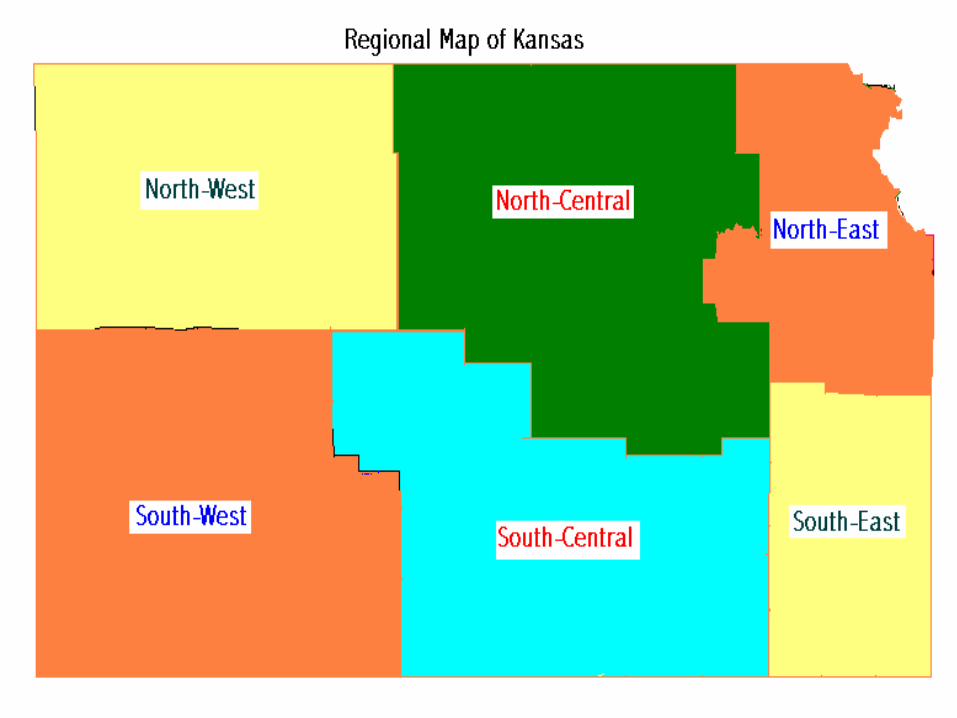
Average % Market Share by Region In Kansas

Region Average % Market Share

Region Average % Market Share

Northeast 43.6% Southeast 5.4%

North Central 10.9% South Central 30.9%

Northwest 3.5% Southwest 5.7%

% Market Share Regional Growth Rate

Region Regional Growth Rate

Region Regional Growth Rate

Northeast 1.19% Southeast -0.58%

North Central -0.75% South Central -1.06%

Northwest -1.30% Southwest -0.57%

Model for County Retail Strength

County Retail Strength = f(CB,BP,RE) Where

CB stands for the customer base served BP stands for buying the power of the

customer base RE stands for the retail environment

Pull Factor Regression Analyses

Dependent variable: Pull Factor.

Method: Least Squares.

Included observations: 93.

Variable Names, Predicted Values and Description

Variable Name

Expected Value

Description

PER CAPITA INCOME

+ Measure of the 2002 per capita income in every county

URBAN MASS

+ Population of the dominant city(s) within each county.

VALUE + Measures the per capita value of commercial property in all its dimensions: both real and personal property.

CIIV + The size of the flow of commuter income.

MJRHWY + Indicates whether a county is on a major highway

Pull Factor Regression Analyses (contd…)

Variable Coefficient Std.error t-Stat Probability

CIIV 0.14882 0.05321 2.7965 0.0064

INCOME 0.02127 0.00669 3.1775 0.0021

MJRHWY 0.07131 0.03560 2.0029 0.0483

URBANMASS 0.00259 4.37E-4 5.9300 0.0000

VALUE 0.00027 5.61E-5 4.9496 0.0000

Pull Factor Regression Analyses (contd…)

R-squared 0.7574

Adjusted R-squared 0.7434

Sum of squared errors 1.4315

Log likelihood 62.1226

Mean dependent variable 0.61075

Schwarz criterion 0.02062

Akaike Information criterion 0.01751

Economic Development Strategies and Resources

STRATEGIES Human Capital

Financial Capital

Social Capital

Engineered Capital

Environmental & Natural Resource Capital

Retentions & Expansion

Firm Creation

Local Linkage

Capture Dollar

Attraction

Thomas County Example:

Thomas County

Popl’n 2001

Pull

Factor

Trade Area Capture

% of county Sales

Colby 5,251 1.38 7,248 80.24

Brewster 280 0.20 57 0.63

Rexford 156 0.09 14 0.16

Gem 95 0.02 2 0.02

Menlo 57 0.05 3 0.03

Rest of County 2,069 0.82 1,692 18.73

County Data 7,962 1.13 9,032 100.00

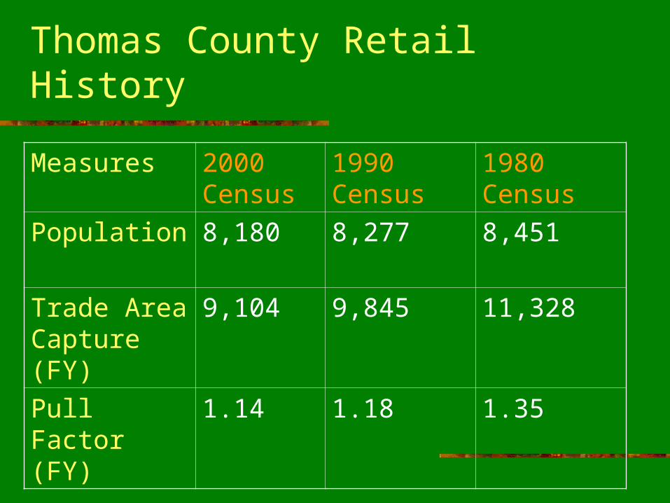
Thomas County Retail History

Measures 2000 Census

1990 Census

1980 Census

Population 8,180 8,277 8,451

Trade Area Capture (FY)

9,104 9,845 11,328

Pull Factor (FY)

1.14 1.18 1.35

Firm Marketing Choices

1. Expand market share with the current product line.

2. Enter a new market with the current product line.

3. Develop a new product for the current market.

4. Develop new product and sell in a new market.

Further Research Needed

If retail sales are a derived demand, what do retail sales measure?

Who are the stakeholders in a successful retail community?

Should local governments subsidize it? Should economic developers spend their

time and efforts assisting retail businesses?

Policy Issues

Should retail sales be taxed? If so, how should we tax Internet and

catalogue sales? Should government subsidize small retail

operations the way it subsidizes farm businesses? Why? Why not?

For more information go to: www.agecon.ksu.edu/ddarling