AIAA 2000-0393

The CE/SE Method for Navier-Stokes Equations Using Unstructured Meshes for Flows at All Speeds

Zeng-Chan Zhang1 and S.T. John Yu2 Mechanical Engineering Department

Wayne State University, Detroit, MI

Xiao-Yen Wang3 Department of Aerospace Eng. and Mechanics

University of Minnesota Minneapolis, MN

Sin-Chung Chang4

NASA Glenn Research Center Cleveland, OH

Ananda Himansu5 Taitech Inc.,

NASA Glenn Research Center Cleveland, OH

Philip C.E. Jorgenson6 NASA Glenn Research Center

Cleveland, OH

1 Visiting Professor from Tsinghua University, China, Email: zz9@nova.eng.wayne.edu 2 Associate Professor, AIAA Member, Email: styu@me1.eng.wayne.edu 3 Research Scientist, AIAA Member, Email: wangxy@aem.umn.edu 4 Senior Aerospace Engineer, Email: sin-chung,chang@lerc.nasa.gov 5 Senior Scientist, Email: fshiman@trout.lerc.nasa.gov 6 Senior Aerospace Engineer, Email: aejorgen@lerc.nasa.gov

Abstract In this paper, we report an extension of the Space-Time Conservation Element and Solution Element (CE/SE) Method for solving the Navier-Stokes equations. Numerical algorithms for both structured and unstructured meshes are developed. To calculate the viscous flux terms, a ‘midpoint rule’ is used. In the setting of space-time flux conservation, a new and unified boundary-condition treatment for solid wall is introduced. The Navier Stokes solvers retain all favorable features of the original CE/SE method for the Euler equations, including high fidelity resolution of unsteady flows, easy implementation of non-reflective boundary conditions, and simplicity of computational logic. In addition, numerical results show that the present Navier-Stokes solvers can be used for high-speed flows as well as low-Mach-number flows without preconditioning. The present Navier Stokes solvers are efficient, accurate, and very robust for flows at all speeds.

1. Introduction The Space-Time Conservation Element and Solution Element Method, or the CE/SE Method for short, originally proposed by Chang [1-6], is a novel numerical framework for conservation laws. The CE/SE method has many non-traditional features, including a unified treatment of space and time, the introduction of conservation element (CE) and solution element (SE), and a shock capturing strategy without Rieman solver. Moreover, the CE/SE method is based on triangles and

tetrahedrons for two- and three-dimensional flows. Thus it is naturally suited for unstructured mesh. As such, the CE/SE method is a genuine multidimensional scheme because the method has been constructed without dimensional splitting. To date, numerous highly accurate solutions have been reported, including traveling and interacting shocks, acoustic waves, shedding vortices, detonation waves, shock/acoustic waves interaction, shock/vortex interaction, and cavitating flows. In this paper, the CE/SE method is extended for solving the Navier-Stokes equations. The rest of the paper is organized as follows.

In the beginning of Section 2, a short summary for the CE/SE method for the Euler equations in two spatial dimensions is provided. The CE/SE scheme for the Navier-Stokes equations will then be presented. In Section 3, a new and unified wall boundary treatment (proposed by Chang), which is based on space-time flux conservation near wall, is introduced. This wall boundary condition treatment is accurate and numerically stable. In Section 4, we present several flow solutions in a wide range of speeds obtained by the CE/SE Navier Stokes solver. All results compared favorably with reported experimental data or previous numerical solutions. A three-dimensional result by the CE/SE method is also reported. We then offer concluding remarks and give the list of cited references.

2

2. The CE/SE Viscous Scheme

Consider the following two-dimensional Navier-Stokes Equations, its dimensionless conservation form can be written as

0=∂

∂−∂

∂−∂

∂+∂∂+

∂∂

yG

xF

yg

xf

tU vmvmmmm , (2.1)

where m =1, 2, 3, 4 indicating the continuity, two momentum and the energy equations. Here f and g are the inviscid parts of the fluxes, and they are functions of Um. Fv and Gv are viscous parts of the fluxes, which are functions of Um, Uxm and Uym. Let x1 = x, x2 = y and x3 = t be the coordinates of a three-dimensional Euclidean space E3. The integral counterpart of Eq. (2.1) is

0)(

=⋅∫ VS m dsH , m = 1, 2, 3, 4 (2.2)

Here Hm=(fm-Fvm, gm-Gvm, Um) are the space-time current density vectors of mass, x-momentum, y-momentum and energy, respectively. S(V) is the boundary surface of a space-time region V in E3. The above flux vector Hm can be decomposed into the inviscid and viscous parts:

vmmm HhH −= (2.3) with

hm = (fm, gm, Um), (2.4a) Hvm = (Fvm, Gvm, 0), (2.4b)

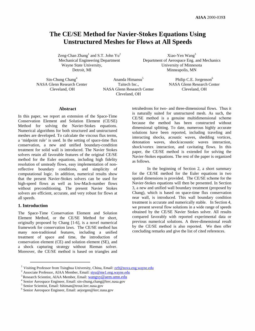
In two spatial dimensions, triangular spatial mesh is used to perform space-time integration. Refer to Fig.1. The grid points are located at centers of triangles. At each mesh node, three conservation elements (CEs) and one solution element (SE) are defined in connection with its three neighbors. For example, at point G, three CE(l) (l = 1, 2, 3) are the cylinders EFGDE′F′G′D′ (CE(1)), ABGFA′B′G′F′ (CE(2)) and CDGBC′D′G′B′ (CE(3). The SE is the union of four planes ABCDEF, G′G′′B′′B′, G′G′′D′′D′, G′G′′F′′F′ and their immediate neighborhood.

Inside each SE(j, n), the flow variables are assumed continuous. By using the first-order Taylor series expansions, Um(x, y, t) , fm(x, y, t) and gm(x, y, t) are approximated by,

+−+= )()()(),;,,(*j

njmx

njmm xxUUnjtyxU

)()()()( nnjmtj

njmy ttUyyU −+−+ (2.5a)

+−+= )()()(),;,,(*

jnjmx

njmm xxffnjtyxf

)()()()( nnjmtj

njmy ttfyyf −+−+ (2.5b)

+−+= )()()(),;,,(*

jnjmx

njmm xxggnjtyxg

)()()()( nnjmtj

njmy ttgyyg −+−+ (2.5c)

Accordingly, ),,;,,((),;,,( ** njtyxfnjtyxh mm =

)),;,,(),,;,,( ** njtyxUnjtyxg mm (2.6)

G

B

DF

( a )

A'C'

E'

F''

E''C''

B''

A''

G''

G

A

B

C

D

E

F

A'

F'B'

D'

E'C'

G'

D''

t/2

t/2

( b )

n

n-1/2

n+1/2

S

Q

A

F'

A'

F

n-1/4

n-1/2

n

( c )

Fig. 1 A schematic of the CE/SE scheme: (a) triangle mesh in two spatial dimensions; (b) The definitions of the CEs and SE; (c) the calculation of the space-time flux.

Thus Eq.(2.2) can be calculated by using the dicrete form:

0)()),((

*)(

=⋅−∫ njCES vmmldsHh , (2.7)

where S(CE(l)(j,n)) is the boundary surface of CE(l).

To proceed, we illustrate the viscous term integral in Eq. (2.7). From Eq. (2.4b), the third component of Hvm in time is null. Thus, in calculating the viscous fluxes, we only need to calculate integrals over lateral surfaces in the space-time domain. For example, in calculating viscous flux over CE(2), the quadrilateral cylinder ABGFA′B′G′F′, we only need to calculate the integrals of viscous terms over four lateral surfaces ABA′B′, AFA′F′, GBG′B′ and GF′G′F′. As shown in Fig.1(c), we define the surface vector, denoted by ),,( tyx SSSS =∆

�

, for the surface

AFA′F’ as the unit outward normal vector multiplied by its area. Thus we have

)),,(( 4/1

''

−⋅≈⋅∫nQmymxmvmx

FAFAvm UUUFSdSH

)),,(( 4/1−⋅+ nQmymxmvmy UUUGS (2.8)

3

where Q is the centroid of AFA′F′. Because the surface AFA′F′ belong to the SE of point A′, we have

+−+≈ −−− )()()()( '2/1

'2/1

'4/1

AQnAmx

nAm

nQm xxUUU

2/1''

2/1' )(4/)()( −− ⋅∆+−+ n

AmtAQnAmy UtyyU (2.9)

To calculate (Umx)Q and (Umy)Q, we assumed a linear distribution of U in the SE, and the following approximation is employed:

2/1'

4/1 )()( −− ≈ nAmx

nQmx UU ;

2/1'

4/1 )()( −− ≈ nAmy

nQmy UU (2.10)

It is similar for surface AFA′F′. But for surfaces GBG′B′, GDG′D′ and GF′G′F′, because they belong to the SE of point G, and they also belong to the SE of point G′, we can use the flow variables Um, Umx and Umy at point G or G′ to approximate the Um, Umx and Umy at the centroid of each surface. We note that as an approximation it is more efficient to use the flow variables and their derivatives at point G′, which is located at previous time step, such that we need not solve nonlinear equations for Umx and Umy at each grid point at the new time level. In this case, however, we must use the dual mesh.

To proceed, we substitute Eqs. (2.5) and (2.6) into Eq. (2.7), and obtain the following discrete equations:

[ ] [ ] 2/1

,321321

−−−−+++∑∑∑∑∑∑ ++=++

n

ljylxlln

jylxll UUUUUU������

(2.11) where l =1,2,3 for flux conservation over three CEs. By adding the three equations together, we get the final formulation for the numerical solution of the flow variables U

�

:

[ ]2/1

,

3

1321

1 −

=

−−−∑ ∑∑∑ ++=

n

ljlylxll

h

nj UUU

SU

���� (2.12)

By solving any two of Eqs. (2.11), we can obtain the numerical solutions for n

jxU )(�

and njyU )(

�

, which we

denote as nj

axU )(

�

and nj

ayU )(

�

.

Equation (2.12) for U�

, in conjunction with two of the three equation expressed by Eqs (2.11) for xU

�

and yU

� , are the space-time CE/SE scheme for solving the two-dimensional Navier-Stokes equations. This is similar to the a-scheme for Euler equations [1-6]. Using the same method as that in [1-6], we can get the a-ε and the a-ε-α-β schemes for the Navier Stokes solver. Since the above scheme is based on triangles, it can be directly used in unstructured mesh. In addition, the above scheme can be extended to three-dimensional case in a straight way.

3. Wall Boundary Treatment In the setting of the CE/SE method, a new boundary condition treatment is developed based on space-time flux conservation. The idea was proposed by Chang, the fourth author of the present paper. Here, only a brief account of this treatment is provided.

G

E

A

B

C

D F

CE(1)

CE(2)CE(3)

y

x (a)

t

y

x

A'

AB

C

D

E

F

G

B'

C'

D'

E'

F'

G'

(b)

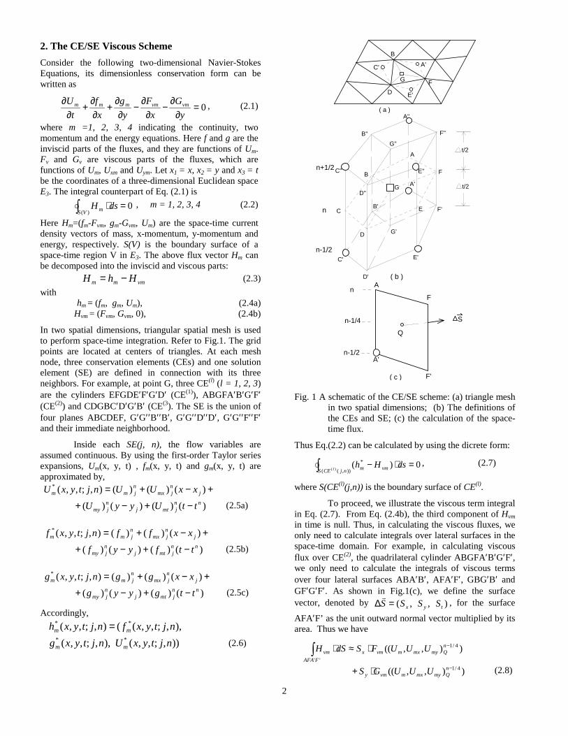
Fig.2. A schematic for wall boundary treatmnet: (a)

Spatial mesh and (b) CEs near the wall boundary.

In the traditional wall boundary treatment, the slip condition is applied along the wall for inviscid flows, while non-slip condition is applied for viscous flows. One cannot make any connection between these two treatments. In the setting of the Space-Time CE/SE method, a new and unified wall boundary treatment is proposed for solving the Navier-Stokes equations. Essentially, the shear stress exerted on the fluid by a wall is modeled as a source term as a part of the local space-time flux conservation over a conservation element in the vicinity of the wall boundary. When the fluid is inviscid, the source term vanishes and the boundary condition reduces to the usual “slip” condition along the wall. When the flow is viscous, the source term survives and the boundary condition is fully consistent with the traditional non-slip condition.

Figure 2(a) shows a schematic of the grid points near a horizontal wall. No grid point is placed on the wall. Instead, a ghost point E, which is the mirror image of point G with respect to the wall, is used. The flow variables Ui, (i = 1, 2, 3, 4) (U = (ρ, ρu, ρv, Et) for two-dimensional flows) and their spatial derivatives, (Ux)i and (Uy)i ( i = 1, 2, 3, 4), at point E are obtained from those of point G by assuming that, at any time t, the flow fields below and above DF are the mirror images of each other. Note that the mirror-image conditions traditionally are applied to inviscid flows but not viscous flows. Here, they are applied to both inviscid and viscous flows. With these conditions specified on the ghost point, we can calculate the flow variables and their spatial derivatives at point G for the

4

next time step. In the CE/SE method, this calculation is carried out by the space-time integration over three conservation elements CE(i), i =1,2,3 (Fig.2(b)). Additional treatment for the space-time flux calculation in CE(1) is needed due to the existence of the wall boundary lying across the conservation element.

Let (i) the viscosity µ be a constant; and (ii) the wall be an insulated wall. Because (i) u = v = 0 at the wall; and (ii) the numerical solution is linear in x, y, and t within a solution element, it can be shown that the mass, x-momentum, y-momentum and energy fluxes entering into the fluid in the triangular cylinder GDFG′D′F′ from the wall form the row matrix

++ ∂

∂⋅−∂∂⋅−⋅= Q

eLeLw y

vR

pyu

RSf )0,

34,1,0(

� (3.1)

On the other hand, the same four fluxes entering into the fluid in the triangular cylinder EFDE′F′D′ from the wall form the row matrix

−− ∂∂⋅−

∂∂⋅−⋅−= Q

eLeLw y

vR

pyu

RSf )0,

34,1,0(

� (3.2)

Note that, in Eqs. (3.1) and (3.2), (i) S is the area of the surface DFF′D′; and (ii) the fluid properties associated with

+wf�

and −wf

�

, respectively, are to be evaluated at points Q+ and Q-, which, respectively, are immediately above and below the centroid Q of the rectangle DFF′D′. Using the mirror image conditions, we have

+− ∂∂−=

∂∂

QQ yu

yu )()( ,

+− ∂

∂−=∂∂− Q

eLQ

eL yv

Rp

yv

Rp )

34()

34( (3.3)

By using Eqs. (3.1)-(3.3), it is concluded that the total mass, x-momentum, y-momentum and energy fluxes entering into the fluid in the cylinder GDEFG′D′E′F′ (i.e., CE(1)) from the wall form the row matrix

+−+ ∂∂⋅⋅−=+= Q

eLwww y

uR

Sfff )0,0,1,0(2��� (3 .4)

In the current treatment, the surviving x-momentum flux in Eq. (3.4) is treated as a source term in flux balance calculation involving conservation element CE(1). To calculate the flux wf

�

, we need to calculate ∂u/∂y. For simple laminar flows with enough mesh resolution of the boundary layer, because u = 0 at point Q+, and u ≅ (uG + uG′)/2 at the midpoint M of 'GG , we can assume that,

++

−−+

≈

∂∂

QM

GG

Q yyuu

yu 02/)( ' (3.5)

Note that, for the inviscid flows (i.e., 1/ReL = 0), 0=wf�

. Thus the current boundary treatment becomes the usual “slip” condition because only the mirror-image conditions are imposed. As such, the present boundary treatment is a unified one, suitable for inviscid as well as viscous flows.

4. Numerical Results To demonstrate the capabilities of the present scheme, several flow problems are calculated.

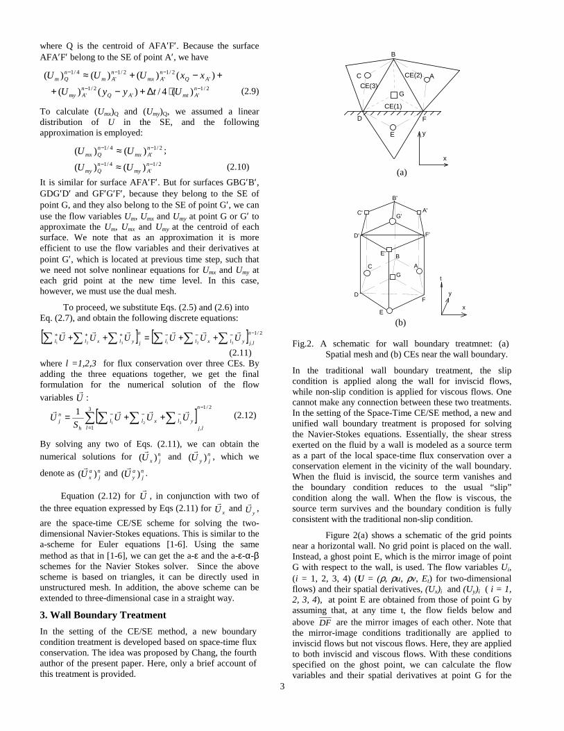
4. 1 Shock/Boundary Layer Interaction The first problem is the shock/boundary layer interaction, which is a standard test problem for Navier Stokes solvers. When the shock is strong and the incident shock angle is large, boundary layer separation occurs at the shock impinging point. In order to resolve the boundary layer, clustered cells near the solid wall must be employed.

incident shock

reflective shock

Fig.3 Shock/boundary layer interaction.

The free-stream Mach number is M∝ =2.0. The Reynolds number Re=2.96×105. The shock incident angle β=32.6o. The computational domain is [0, 0.12]×[0, 0.06] and 38400 triangles are used.

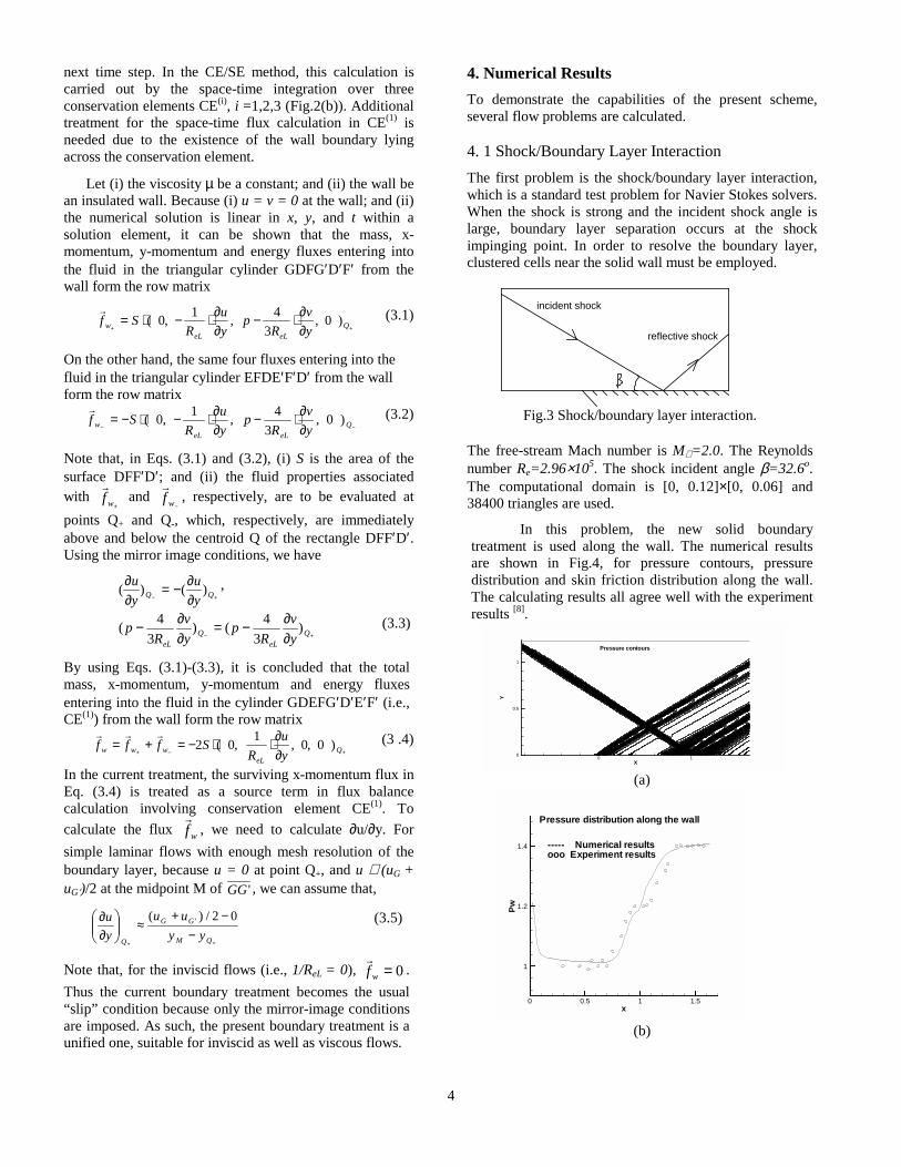
In this problem, the new solid boundary treatment is used along the wall. The numerical results are shown in Fig.4, for pressure contours, pressure distribution and skin friction distribution along the wall. The calculating results all agree well with the experiment results [8].

0 1

X0

0.5

1

Y

Pressure contours

(a)

0 0.5 1 1.5

x

1

1.2

1.4

Pw

Pressure distribution along the wall

----- Numerical resultsooo Experiment results

(b)

5

0 0.5 1 1.5x

-1

0

1

2

3

4

CfX

1000

Skin friction distribution along the wall

------ Numerical resultsooo Experiment data

( c)

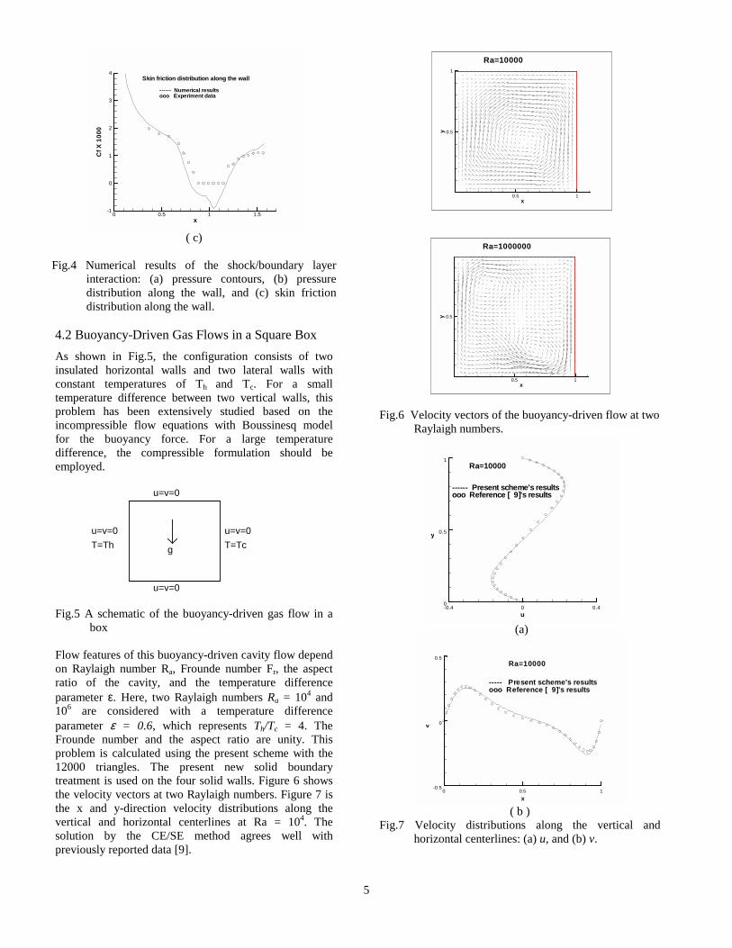
Fig.4 Numerical results of the shock/boundary layer

interaction: (a) pressure contours, (b) pressure distribution along the wall, and (c) skin friction distribution along the wall.

4.2 Buoyancy-Driven Gas Flows in a Square Box As shown in Fig.5, the configuration consists of two insulated horizontal walls and two lateral walls with constant temperatures of Th and Tc. For a small temperature difference between two vertical walls, this problem has been extensively studied based on the incompressible flow equations with Boussinesq model for the buoyancy force. For a large temperature difference, the compressible formulation should be employed.

g

u=v=0

u=v=0

u=v=0T=Th

u=v=0T=Tc

Fig.5 A schematic of the buoyancy-driven gas flow in a

box Flow features of this buoyancy-driven cavity flow depend on Raylaigh number Ra, Frounde number Fr, the aspect ratio of the cavity, and the temperature difference parameter ε. Here, two Raylaigh numbers Ra = 104 and 106 are considered with a temperature difference parameter ε = 0.6, which represents Th/Tc = 4. The Frounde number and the aspect ratio are unity. This problem is calculated using the present scheme with the 12000 triangles. The present new solid boundary treatment is used on the four solid walls. Figure 6 shows the velocity vectors at two Raylaigh numbers. Figure 7 is the x and y-direction velocity distributions along the vertical and horizontal centerlines at Ra = 104. The solution by the CE/SE method agrees well with previously reported data [9].

0.5 1x

0.5

1

y

Ra=10000

0.5 1

x

0.5y

Ra=1000000

Fig.6 Velocity vectors of the buoyancy-driven flow at two

Raylaigh numbers.

-0.4 0 0.4u

0

0.5

1

y

Ra=10000

------ Present scheme's resultsooo Reference [ 9]'s results

(a)

0 0.5 1x

-0.5

0

0.5

v

Ra=10000

----- Present scheme's resultsooo Reference [ 9]'s results

( b )

Fig.7 Velocity distributions along the vertical and horizontal centerlines: (a) u, and (b) v.

6

4.3 Driven Cavity Flow This problem is a benchmark problem for incompressible viscous flow calculations. Here the full compressible Navier-Stokes equations are solved to demonstrate the capabilities of the CE/SE scheme at the incompressible limit. Here the 12000 triangles are used. Figure 8 shows velocity vectors, x and y-direction velocity distributions along the vertical and horizontal centerlines at Re = 103. This solution agrees well with Ghia’s data [10].

0.5 1x ( a )

0.5

1

y

Re = 1000

-0.5 0 0.5 1u ( b )

0

0.5

1

y

------ Numerical resultsooo Ghia's data

Re = 1000

0 0.5 1x ( c )

-0.5

0

0.5

v

Re = 1000

------ Numerical resultsooo Ghia's data

Fig.8. Solution of a driven cavity flows: (a) Velocity vectors, (b) u along the vertical centerline, and (c) v along the central horizontal centerline.

4.4 Flows Over a Circular Cylinder The fourth example is an external flow over a circular cylinder at Re = 40, with which a steady state solution exists. Again, the full compressible equations are solved by the CE/SE method without preconditioning. The computational domain is [-5,15]×[-5, 5], and 10,092 triangles are used. Figure 9(a) shows the unstructured mesh near the circular cylinder. Figure 9(b) shows the velocity vectors of the flow solution. The wake length L/d≈2.0, and it compares well with the experiment data and previously reported results [11].

-1 0 1

X ( a )

-1

0

1

Y

( b )

Fig.9. A flow over a cylinder (Re = 40): (a) the mesh around the cylinder, (b) velocity vectors.

X Y

Z

y=0.5

7

X

Y Z

z=0.5

Fig.10. Velocity vectors in the mid-planes (y=0.5 and

z=0.5) of a three-dimensional driven cavity flow. 4.5 A Three-Dimensional Driven Cavity Flow The top lid is moving in the x direction with a constant speed with Re=500. 124,992 tetrahedrons are used. Figure 10 is the velocity vectors in the mid-plane y=0.5 and z=0.5. This result at y=0.5 plane is very similar to its two-dimensional counterpart. Details of the three-dimensional CE/SE method for Navier-Stokes equations will be presented in a separate paper.

Concluding Remarks In this paper, we report an extension of the space-time CE/SE method for Navier Stokes equations. This scheme retains all favorable features of the CE/SE method, including the unified treatment of space and time, accurate computation of space-time flux conservation, and high resolution of unsteady flows. Since the present CE/SE method is based on triangles and tetrahedrons for two and three-dimensional flows, it is naturally suited for unstructured meshed. A unified wall boundary condition treatment for inviscid as well as viscous flows is illustrated. The present Navier Stokes solver of the CE/SE scheme can be applied to high speed flows as well as low-Mach-number flows without preconditioning. Numerical results reported in this paper agree well with the experimental or previously reported numerical results.

Acknowledgement This work is performed under the support of NASA Glenn Research Center NCC3-580. This work is also a part of an ongoing program at Wayne State University in applying the Space-Time CE/SE Method to practical engineering problems.

References 1. Chang, S.C., “The Method of Space-Time

Conservation Element and Solution Element – A New Approach for Solving the Navier Stokes and Euler Equations,” J. Comp. Phys., 119, 1995, pp. 295-324.

2. Chang, S.C., Wang, X.Y. and Chow, C.Y. “The Space-Time Conservation Element and Solution Element Method: A New High-Resolution and Genuinely Multidimensional Paradigm for Solving Conservation Laws,” J. Comp. Phys., 156, 1999, pp. 89-136.

3. Wang, X.Y. and Chang, S.C., “A 2D Non-Splitting Unstructured Triangular Mesh Euler Solver Based on the Space-Time Conservation Element and Solution Element Method,” Computational Fluid Dynamics J., 8 (2), 1999, pp. 309-325.

4. Chang, S.C., Yu, S.T., Himansu, A., Wang, X.Y., Chow, C.Y. and Loh, C.Y., “The Method of Space-Time Conservation Element and Solution Element – A New Paradigm for Numerical Solution of Conservation Laws,” Computational Fluid Dynamics Review, 1, 1998, pp. 206-240. Editors: Hafez, M. and Oshima, K., World Scientific Publisher.

5. Chang, S.C. and Himansu, A., “The Implicit and Explicit a-µ Schemes,” NASA/TM 97-206307, 1997.

6. Chang, S.C., Himansu, A., Loh, C.Y., Wang, X.Y., Yu S.T., Jorgenson, P., “Robust and Simple Nonreflecting Boundary Conditions for the Space-Time Conservation Element and Solution Element Method,” AIAA Paper 97-2077, the 13th AIAA CFD Conference, June 1997, Snow Mass, CO.

7. Wang, X.Y., “Computational Fluid Dynamics based on the Method of Space-Time Conservation Element and Solution Element,” Ph.D. Dissertation, Univ. of Colorado at Boulder, 1995.

8. Hakkinen, R.J., Greber, I., Trilling, L. and Abarbanel, S.S., “The Interaction of an Oblique Shock Wave with a Laminar Boundary Layer,” NASA Memo 2-18-59W, 1959.

9. Yu, S.T., Jian, B.N., Wu, J. and Liu, N.S., “A div-curl-grad formulation for compressible buoyant flows solved by the least-squares finite element method,” Comput. Methods Appl. Mech. Engrg., 137, 1996, pp. 59-88.

10. Ghia, U., Ghia, K.N. and Shin, C.T., “High-Re Solutions for Incompressible Flow Using the Navier-Stokes Equations and a Multigrid Method,” J. Comp. Phys., 48, 1982, pp. 387-411.

11. Dennis, S.C.R. and Chang, G.Z., “Numerical Solutions for Steady Flow Past a Circular Cylinder at Reynolds Numbers up to 100,” J. Fluid Mechs., 42, 1970, 471-489.

12. Wang, X.Y. and Chang, S.C., “A 3-D Non-Splitting Structured and Unstructured Euler Solver Based on the Space-Time Conservation Element and Solution Element Method,” AIAA Paper 99-3278, June. 1999.

13. Zhang, Z.C., Yu, S.T., Chang, S.C., Himansu, A. and Jorgenson, P., “A Modified Space-Time CE/SE Method for Euler and Navier-Stokes Equations,” AIAA Paper 99-3277, June. 1999.

14. Zhang, Z.C. and Yu, S.T., “Shock Capturing without Riemann Solver---A Modified Space-Time CE/SE Method for Conservation Laws,” AIAA Paper 99-0904, Jan. 1999.