THE CENTRE FOR MARKET AND PUBLIC ORGANISATION

Centre for Market and Public Organisation University of Bristol

2 Priory Road Bristol BS8 1TX

http://www.bristol.ac.uk/cmpo/

Tel: (0117) 33 10952 Fax: (0117) 33 10705

E-mail: cmpo-admin@bristol.ac.uk The Centre for Market and Public Organisation (CMPO) is a leading research centre, combining expertise in economics, geography and law. Our objective is to study the intersection between the public and private sectors of the economy, and in particular to understand the right way to organise and deliver public services. The Centre aims to develop research, contribute to the public debate and inform policy-making. CMPO, now an ESRC Research Centre was established in 1998 with two large grants from The Leverhulme Trust. In 2004 we were awarded ESRC Research Centre status, and CMPO now combines core funding from both the ESRC and the Trust.

ISSN 1473-625X

The Socioeconomic Gradient in Physical Inactivity in England

Lisa Farrell, Bruce Hollingsworth, Carol Propper and Michael A.

Shields

July 2013

Working Paper No. 13/311

CMPO Working Paper Series No. 13/311

The Socioeconomic Gradient in Physical Inactivity in England

Lisa Farrell1, Bruce Hollingsworth2, Carol Propper3 and Michael A. Shields4

1RMIT University

2Lancaster University

3Imperial College London, Bristol University and CEPR

4Monash University

July 2013

Abstract Physical inactivity is recognised as an important precursor of chronic ill health. It is also recognised as a modifiable health behaviour, so knowing who is physically inactive is important for design of policy interventions to reverse the increase in physical inactivity. Studies examining the correlates of physical inactivity have identified socioeconomic position and aspects of the geographical environment as important. In this paper we contribute to this literature by exploiting detailed data on over one million individuals in England to more precisely identify and separate the associations between several measures of physical inactivity, different aspects of socioeconomic position and a wide range of local geographical factors. Our results show high levels of physical inactivity and clear separate associations with important dimensions of socioeconomic position. Education, household income and local area deprivation are all independently and strongly associated with inactivity, controlling for local availability of physical recreation and sporting facilities, the local weather and regional geography. Importantly, local area facilities and geographical factors explain very little of the variation in physical inactivity in England. Further, the income gradient increases with age and more financially costly forms of physical activity are associated with larger socioeconomic position differences, suggesting that financial as well as cultural barriers need to be overcome to reduce inactivity prevalence. Keywords: Physical inactivity, socioeconomic gradient Electronic version: www.bristol.ac.uk/cmpo/publications/papers/2013/wp311.pdf Address for correspondence CMPO University of Bristol 2 Priory Road Bristol BS8 1TX Cmpo-admin@bristol.ac.uk www.bristol.ac.uk/cmpo/

1

The Socioeconomic Gradient in Physical Inactivity in England

Lisa Farrell RMIT University

Bruce Hollingsworth Lancaster University

Carol Propper

Imperial College London, Bristol University and CEPR

Michael A. Shields Monash University

12th July 2013

Abstract Physical inactivity is recognised as an important precursor of chronic ill health. It is also recognised as a modifiable health behaviour, so knowing who is physically inactive is important for design of policy interventions to reverse the increase in physical inactivity. Studies examining the correlates of physical inactivity have identified socioeconomic position and aspects of the geographical environment as important. In this paper we contribute to this literature by exploiting detailed data on over one million individuals in England to more precisely identify and separate the associations between several measures of physical inactivity, different aspects of socioeconomic position and a wide range of local geographical factors. Our results show high levels of physical inactivity and clear separate associations with important dimensions of socioeconomic position. Education, household income and local area deprivation are all independently and strongly associated with inactivity, controlling for local availability of physical recreation and sporting facilities, the local weather and regional geography. Importantly, local area facilities and geographical factors explain very little of the variation in physical inactivity in England. Further, the income gradient increases with age and more financially costly forms of physical activity are associated with larger socioeconomic position differences, suggesting that financial as well as cultural barriers need to be overcome to reduce inactivity prevalence. Key words Physical inactivity, socioeconomic gradient

2

1. Introduction

Physical inactivity is increasingly recognised as an important precursor of chronic ill health with

large costs for individuals and society (Das and Horton, 2012). The World Health Organisation

(WHO) estimates that physical inactivity causes 1.9 million deaths per year worldwide, 10 to 16 per

cent of breast cancer, colon cancer and diabetes cases, and about 22 per cent of coronary heart

disease cases (WHO, 2004). Physical inactivity is also recognised as potentially the most important

modifiable health behaviour for chronic disease. Scarborough et al. (2011) argue that of the four

modifiable causes - smoking, alcohol, diet, and lack of physical activity - low physical activity is

the most prevalent chronic disease risk factor. As a result, governments are seeking ways to

decrease physical inactivity (for example, WHO, 2007) and knowing who is physically inactive is

important for designing cost effective policy interventions (Hamer, 2012).

Studies that have examined the correlates of physical inactivity in the developed world have

repeatedly identified socio-economic position (SEP) and aspects of the local geographical

environment as important (Giles-Corti and Donovan, 2002; Humpel et al., 2002; WHO, 2004, 2007;

Frost et al., 2010; van Dyck et al., 2010; Pascual et al., 2013). However, most studies of physical

inactivity (with a couple of notable examples which we discuss below) have been based on

relatively small-scale samples so while they have drawn attention to SEP as a determinant of lack of

physical activity, they have been more limited in their ability to precisely disentangle the individual

association of different facets of SEP and to separately identify local area factors such as lack of

area resources, poor supply of sports facilities and geographical configuration from individual or

household SEP.

In this paper we seek to contribute to this knowledge base by providing evidence from a

unique data set on over one million individuals in England from the Active People Surveys (APS).

The large sample size and the associated geographical identifiers allow us to match in information

on local area attributes including the availability of sport and exercise facilities, green space and the

weather. This detailed local information enables us to obtain precise estimates of the association

between physical inactivity and different aspects of individual SEP, controlling for local

geographical factors that may affect the costs of physical activity. Our data also allow us to examine

an extensive set of physical inactivity measures that we employ, allowing us to check that our

results are not sensitive to the exact definition of inactivity and to consider the role of cost as well

as income.

Our analyses show the following. First, levels of physical inactivity in England are very

high. About 8 per cent of the adult population that can walk do not even walk for five minutes

continuously in a four-week period. Nearly 80 per cent do not hit key national government targets.

Second, whatever aspect of SEP is considered, there are significant SEP differences that increase

3

monotonically in terms of disadvantage. There is a large socioeconomic gradient even for activities

that have low direct cost (for example walking) and the more costly the activity, the larger the

socioeconomic gradient. Third, different aspects of SEP disadvantage (education and household

income) are independently associated with a lack of physical activity, controlling for local

availability of facilities, weather and geography. Fourth, these differences are already evident in

young adults, but they steadily increase with age. Finally, while local area characteristics are

significant and the direction of their impact appears sensible, they explain very little of the

differences in activity levels over and above individual and household characteristics.

2. Background

2.1. Health consequences of physical inactivity

The importance of walking and physical activity as determinants of good health has been well

established in the medical and public health literature (see, for example, U.S. Department of Health

and Human Services, 1996; WHO, 2002). The WHO has identified physical inactivity as a leading

global risk factor for morbidity and premature mortality (WHO, 2004). Das and Horton (2012)

argue that lack of physical activity is a major risk factor in non-communicable disease (NCD)

internationally and note that landmark papers published in The Lancet in 1953 first showed the

association between physical inactivity and heart disease (Morris et al., 1953a,b). Inactivity has

been identified as a risk factor for a number of serious health issues including cardiovascular

disease, type 2 diabetes, obesity, some cancers, poor skeletal health, poor mental health, and overall

mortality (Hallal et al., 2012). It is estimated one third of deaths are caused by diseases which

could, at least in part, be impacted upon by increased physical activity (Allender et al., 2007) and

Min Lee et al. (2012) suggest that the number of deaths due to a lack of physical activity is

approximately the same number of deaths as caused by tobacco. Gregory and Dhaval (2013) found

that physical activity has a durable impact on health.

The first US Surgeon General’s Report on Physical Activity and Health, released almost

twenty years ago in 1996, recommended that adults engage in thirty minutes of moderate physical

activity at least five days per week. Subsequently these limits have been raised in the US, Canada

and the UK (Physical Activity Guidelines Advisory Committee, 2008; Tremblay et al., 2008; Bull

et al., 2010). However, Das and Horton (2012) argue that lack of physical activity is still neglected

in importance compared to other risk factors, such as tobacco, diet, and alcohol. Wen and Wu

(2012) also note the lack of concern over physical activity levels and make a comparison with the

campaign against smoking, where doctors emphasize the harm and there are international actions to

control tobacco consumption (e.g. WHO, 2003).

4

2.2. Physical inactivity and socioeconomic position (SEP)

Inactivity and obesity are not just public health problems. They are also economic and cultural

phenomenon and so are likely to be differentially patterned by SEP. There are many routes by

which SEP may be associated with inactivity. First, physical activity has a direct cost. Philipson

(2001) argues that long-term technological change in methods of production means that the cost of

expending calories has increased because physical labour has been replaced by machine labour. A

hundred years ago, individuals were paid to do physical work, while currently individuals have to

pay to exercise. As a consequence, sedentary leisure industries are growing at a rate faster than

GDP growth (Sturm, 2004). However, the costs of these changes are not born equally. Paying to

exercise represents a higher proportion of the budget of a poor than a rich individual and low-

income individuals may be very time constrained because their rate of pay per hour is low. As a

consequence, both the direct and the indirect financial costs of activity are higher for individuals

with lower incomes.

Second, from a health production perspective (Grossman, 2006), education increases the

productivity of a given set of healthcare and other inputs, so greater education enables individuals

to increase the amount of physical activity from a given set of resources (either their own or ones

around them). From a more sociological and public health perspective the association between

health knowledge and education (Cutler and Lleray-Muney, 2006) means that individuals who are

better educated may be more aware of the consequences of inactivity and therefore better motivated

to overcome the changes brought about by technological change.

Third, the costs of physical activity will be determined in part by the physical configuration

of the localities in which individuals work and live. Housing markets mean that low-income

individuals tend to live near other low-income individuals and these areas may have poor tax bases

with which to finance recreation and other facilities that enable individuals to take exercise (Moore,

2008; Powell, 2006). These areas are also likely to have fewer general physical and recreational

amenities and higher crime rates that also make physical activity more difficult (Gomez, 2004).

Fourth, as the public health literature has emphasized, there are strong cultural dimensions to

participation in physical activity (Wilbur, 2002; Arredondo, 2012).

2.3. The empirical literature

The empirical literature is large and researchers have drawn attention to the association between

SEP, physical activity and local geography in many different countries and settings. We focus here

on key findings and concerns from recent systematic reviews. Gidlow et al. (2006) undertook a

systematic review of the relationship between physical activity and SEP. Looking at over 25

studies published from 1991 to 2004 (some using data for 20 years earlier) there was consistent

5

evidence of higher prevalence, or higher levels, of activity among those in higher SEPs. Education

was the most commonly used indicator of SEP. Later large cross-national studies have confirmed

this association with education (for example, de Almeida et al. 1999). Education has also been

found to be an important determinant of leisure (as distinct from work) physical activity (for

example, Borodulin et al. (2008) for 4,000 men and women in Finland). Recent studies examining

longitudinal data have also confirmed the importance of education (for example, Hamer et al.,

2012) use the UK Whitehall II cohort study and find a relationship between objective measures of

physical activity and sedentary behavior and levels of education, but not other aspects of SEP).

Gidlow et al. (2006) noted that a small number of studies also reported a gradient across

social classes. However, most of the studies they review used only three categories of social class,

making identification of gradients perhaps somewhat crude. The same overview also found that

when income was used rather than social class, the majority of studies found a positive relationship

between income and physical activity, but again most studies used only three or fewer categories of

income group, making it difficult to identify income gradients.

Studies have also identified the importance of local area factors in a variety of settings.

Parks et al. (2003), in a cross sectional study of 1,818 US adults, found those in rural settings were

less likely to meet recommended levels of physical activity. The importance of environmental

factors, such as places to exercise, also varied across income groups. Pascual et al. (2013) in a case

study in Madrid found availability of sports facilities explained an important part of physical

inactivity. This association between physical activity settings and SEP was also reported by Powell

et al. (2004), who looked at associations across 209 communities in the USA. The HABITAT

multilevel longitudinal study examined associations between neighborhood disadvantage and

physical activity for a sample of 11,037 individuals in 200 neighborhoods in Australia (Turrell et

al., 2010) and found those in advantaged neighborhoods had significantly higher levels of total and

moderate physical activity, as well as walking. However, Giles-Corti and Donovan (2002) in a cross

sectional study of 1,803 Australian adults, found that even when those in lower SEP areas have

superior access to facilities, they are less likely to use them than those resident in higher SEP areas.

Finally, there are studies which draw attention to ethnic differences. Dogra et al. (2010)

using Canadian data show that there are clear preference differences in the modes of physical

activity between Whites and ethnic minorities. Ethnic groups are less active and have a much

smaller and more conventional set of physical activities that they engage in. In the UK, Williams et

al. (2011) conclude that low levels of physical activity among South Asians may be contributing to

their much higher levels of coronary heart disease. A recent study by Saffer et al. (2011) of over

75,000 American adults in 2003-2009 showed that non-work physical activity is significantly lower

for non-white racial groups and for males. Work related physical activity has a negative effect on

6

non-work physical activity, and work related physical activity is significantly lower among Asians

and higher among other groups relative to Whites.

The existing literature also has important limitations. First, education is generally better

measured than income or social class and as a consequence is seen as providing the most robust

results (Gidlow et al., 2006). However, it does not follow from this that income or other measures

of SEP are unimportant. Second, even studies that have adopted explicitly quantitative approaches

tend to suffer from either sample size or sample selection issues. In many cases studies focus only

on one city, identifying variation from between different areas in the city or restrict their attention to

one geographical area (a notable exception is Saffer et al., 2011) 1. In addition, many of the studies

to date have used diverse, and often crude, measures of physical activity and SEP, making it

difficult to establish robust effects. Gidlow et al. (2006) called for further studies using better

measures, drew attention to the use of area level socioeconomic measurement and the need to use

larger samples. This was echoed in a review of the sizeable literature that examines the relationship

between physical activity and its association with neighbourhood attributes, including community

attributes such as crime (Loukatiou-Sideris, 2006).

2.4. Research design

In the present study we exploit a data set containing over one million individuals, representative of

the adult population of England. Our approach has a number of important advantages. First, the

number of observations in our data allows us to establish the patterns in the lack of physical activity

by various correlated aspects of SEP (education, income and local area deprivation) to establish

whether each aspect of SEP contributes independently to differences in inactivity levels. Second,

the data set identifies around 300 separate physical activities so we can focus our study on the most

common physical activities and can undertake separate analyses for physical activities that differ in

their direct cost, allowing us to go some way in separating out a price effect from an income effect.

While we do not observe the monetary price paid for an activity, if there is a price as well as an

income effect, we would expect that income has a greater effect on the lack of participation in

physical activities which are generally accepted as having higher direct costs. Third, the large

sample size means we can examine whether the physical activity gap across SEP increases with age

i.e. we can examine whether there is a significant SEP-age gradient. Fourth, the large size of our

sample means we can separate out the effect of geographical variation in the physical environment

1 For example, van Lenthe et al. (2005) examine the association between the neighbourhood socioeconomic environment and physical inactivity in 78 neighbourhoods of Eindhoven, The Netherlands, with a sample size of 8,767. Harrison et al. (2007) use data from a population-based health and lifestyle survey of adults in northwest England to analyse associations between individual and neighbourhood perceptions and physical activity. The achieved sample was 15,461 and the authors argue this is one of the most comprehensive assessments of individual and contextual associations with physical activity among adults in the UK general population.

7

from individual characteristics by allowing for unobserved time invariant heterogeneity at the local

level. Fifth, we match the respondents to data at the local area level on the availability of sports and

recreation facilities, enabling us to assess whether these supply side factors contribute to a SEP

gradient over and above individual and household characteristics. Finally, England is a good case

study. It is one of the least physically active nations in Europe (de Almeida and Afonso, 1999). By

an objective measure (using accelerometers) only 6 per cent of men and 4 per cent of women reach

the UK’s Department of Health’s recommended levels for activity and over one quarter of the adult

English population is obese and 44 per cent of men and 33 per cent of women are overweight

(Department of Health, 2011).

3. Data description and research design

3.1. Data

The Active People Survey (APS) is collected annually for a large sample of English adults. The

data are cross-sectional and the sampling is clustered at local authority level. Interviews are spread

evenly across the 12 months of each year. The survey is conducted by telephone using Random

Digit Dialing and one person aged 16 or over is randomly selected from eligible household

members. Average response rates are around 25 per cent (we therefore apply population weights in

all our statistical modeling). The survey contains detailed measures of participation in physical

recreation and sport undertaken in the four weeks prior to interview as well as a wide-range of

individual and household level demographic and socioeconomic characteristics.

To date there have been five waves of data released for analysis. The data collection for

each APS runs from October to October, with APS1 (2005-2006), APS2 (2007-2008), APS3 (2008-

2009), APS4 (2009-2010) and APS5 (2010-2011). There is a gap October 2006- October 2007. The

sample sizes were APS1 (n=363,724), APS2 (n=191,325), APS3 (n=193,947), APS4 (n=188,354)

and APS5 (n=166,805), giving a total pooled sample of 1,104,155 individuals aged 16 and over.

The APS5 differed to APS1-4 in that for certain questions only about half of the sample were asked,

including the question on household income. Questions relating to general health status and life

satisfaction were included in APS5 for the first time.2

2 While the data used here are quite unique in their detail and size, they have been little used for research purposes. Sport England (2010) is one of the few quantitative analyses of these data. It uses the APS for one 12 month period (2008/9, n=251,022) and estimates a model of respondents’ achievement of the government’s key national indicator for sports participation (the National Indicator 8 (NI8), defined as “the percentage of the adult population in a local area who participate in sport and active recreation, at moderate intensity, for at least 30 minutes on at least 12 days out of the last 4 weeks”). It finds income, education, household composition, car ownership, and local authority funding to be independently correlated with achieving the NI8 target and also shows that participation in 11 specific sports tends to be associated with different socio-demographic characteristics.

8

There are 354 English local authorities (LAs) identified in APS1-4. The number of LAs was

reduced in APS5 following merging of a number of authorities to 326. We recoded the LAs in

APS1-4 to be consistent with APS5 and thus use variation across 326 LAs here. After eliminating

missing values for the variables used to construct our main physical inactivity measure, as well as

dropping APS5 respondents who were not asked about their household income, we are left with a

working sample of 1,002,219 adults (91 per cent of the total sample). Where there are missing

responses to the variables we use as covariates in our empirical models, we include dummy

indicator variables to control for this non-response.

3.2. Dependent variables

A contribution of this paper is that we construct a number of alternative measures of physical

inactivity. Our primary measure is constructed using information about any types of physical

recreation or sports participation in the last four weeks. At the start of each APS respondents are

asked about their recent walking activities, in particular whether they have done at least one

continuous walk lasting five minutes, which also identifies individuals who report not to be able to

walk3, followed by the number of days in the last four weeks that the respondent has done at least

one continuous walk lasting at least 30 minutes. The intensity (e.g. a ‘slow’ pace; a ‘fast’ pace) of

this walking is also then asked. The same information is then collected for cycling. Both walking

and cycling can include getting to and from work, but the frequency of walking and cycling for

health and recreation only is also separately recorded in the survey. The questionnaire then asks

respondents to think about “other types of sport and recreational physical activity they may have

done, whether it be for competition, training or receiving tuition, socially, casually or for health and

fitness”. Using this information we define physically inactive as reporting not having walked or

cycled for at least 30 continuous minutes at least once in the last four weeks, nor reported

participating in any other type of sport or recreational physical activity of any duration.

We also use information on each type of activity recorded, plus information on the length

and intensity of participation, to construct a number of key participation variables. These are

defined with respect to the UK national indicator of physical activity NI8. We focus on episodes of

at least 30 minutes and of at least moderate intensity. We create three separate variables: (1)

physical activity on no days - denoted KPV=0, (2) physical activity on less than four days (i.e. less

than one episode per week) - denoted KPV<4, and (3) the inverse of the NI8 measure. NI8 tracks

physical activity by looking at people who engage in at least 12 episodes of physical activity at

3 We do not exclude from our sample individuals who are not able to walk (except for our models of walking activity alone) as such a disability does not exclude an individual from all physical activity. Indeed, our data has a rich set of para-sports including: Boccia and wheelchair basketball. We do, however, control for ‘not being able to walk’ and ‘having a chronic limiting condition’ as separate dummy variables as appropriate in our modelling.

9

moderate intensity. As our focus is on inactivity we look at those not achieving the NI8 measure,

i.e. those with less than 12 episodes of physical activity at moderate intensity (an average of less

than three episodes per week) in the last four weeks - denoted KPV<12.

We also examine the constituent parts of our main inactivity measure, distinguishing

between common types of activity, its duration and purpose. The variables we create are whether

the respondent has: (1) not done at least one continuous walk lasting five minutes - denoted “No

Walk 5”, (2) has not done at least one walk of a 30 minute continuous duration for any reason -

denoted “No Walk 30 All”, (3) has not done at least one walk of a 30 minute continuous duration

for health or leisure purposes - denoted “No Walk 30 Leisure”, (4) has not done at least one cycle

ride of a 30 minute continuous duration for any reason - denoted “No Cycling 30 All” and (5) has

not done at least one cycle ride of a 30 minute continuous duration for health or leisure purposes -

denoted “No Cycle 30 Leisure”. We also focus on (absence of) two other common types of physical

activity, (7) swimming - denoted “No Swimming” or (8) using a gym - denoted “No Gym”.

The survey covers a wide range of recreational activities (including gardening) but does not

ask explicitly about occupational physical activity or housework. An analysis of 14,018 adults in

England found the contributions of occupational physical activity to meeting government physical

activity targets to be socially patterned (Allender et al., 2008). When occupational physical activity

was included, men in manual jobs were more likely to meet government targets than those in non-

manual jobs. Similar patterns were observed for women. This omission means that our data may

lead us to under-estimate the amount of physical activity and possibly also over-estimate the SEP

gradient in total physical activity. However, within the large set of common physical activities that

we examine this bias should not be present. Further, to partially circumvent this problem we include

analysis of a very marginal level of the most common physical activity (whether the individual has

walked for five continuous minutes in the last four weeks).

Table 1, final block, presents summary statistics at the individual level for our range of

physical inactivity measures. These confirm the high levels of physical inactivity found in earlier

studies of the UK population. Nearly 20 per cent of the sample did not do any sustained exercise in

a four-week period. In terms of the NI8 target nearly 80 per cent did not meet the criteria of

moderate exercise at least 12 times in a four-week period. Just fewer than 10 per cent (or just over 8

per cent of those who are physically able to walk) of the sample did not even walk for five minutes

continuously in the previous four weeks. Mean levels of participation in even the most common

recreation activities were very low. 46 per cent had not walked for leisure for 30 minutes

continuously, 88 per cent had not swum and 90 per cent had not used a gym.

10

3.3. Covariates

One of our aims is to establish the extent of the relationship between different aspects of SEP and

physical inactivity. To do this we use measures of SEP at the individual, household and LA levels.

Our key individual level measures are highest educational attainment and current employment

status. Our key household measure is annual household income, which is reported in bands in the

APS, and also whether the household resides in council or LA housing (public housing). The other

demographic variables we use are respondent’s (1) age (provided in bands), (2) gender, (3)

ethnicity, (4) family structure (i.e. single adult, children at various ages (0-4, 5-10, and 11-15),

number of individuals in the household), (5) having a chronic health condition, (6) reporting not

being able to walk, and (7) broad occupational grouping for those in work. In our models we also

control for region, survey year, month of interview, and include dummy variables to capture

missing information.

We are also interested in establishing the relationship between local area characteristics (at

the LA level) and physical inactivity. To this end we map to each respondent a range of externally

sourced measures at the LA level. As direct indicators of LA SEP we use the Index of Multiple

Deprivation (IMD) score (which is a measure of deprivation on 6 domains of the LA population);

the LA unemployment rate and the percentage of non-UK British individuals in the LA. We have

information on the extent of the physical nature of the LA – its urbanisation and the percentage of

green space - and on sports facilities. We have data on the number of various types of sports

facilities in the LA per capita and the amount of money received by the LA from the National

Lottery for the purpose of increasing physical activity per capita and from the APS data we

construct a measure of local population satisfaction with the LA recreational facilities. Finally, the

data allow us to identify day of survey interview, which enables us to match weather data on

average rainfall and temperature for the four week period over which the physical activity questions

applied (allowing this to affect the level of outdoor activities conditional on month of the year).4

Descriptive statistics for each variable are shown in Table 1.

3.4. Modeling approach

Our focus is on the association of physical inactivity with key SEP variables at the

individual/household level (highest education, household income) and at the local level (e.g. LA

deprivation). We begin by undertaking simple graphical analysis of the patterns in inactivity. We

4 The Active People Surveys can be accessed through the Data Archive at Essex University. The information on the percentage of green space in each LA was taken from the National Obesity Observatory, as was the information on obesity rates show in Figure 1 (http://www.sepho.nhs.uk). The data on National Lottery awards by LA was provided directly from Sport England, as was data from “Active Places” on sporting and recreation facilities in each LA. The contacts at Sport England can be obtained from the corresponding author, as can the data files subject to permission from Sports England. Weather variables are from the network of national and local weather monitoring stations.

11

then exploit the large scale of our data to examine whether differences we observe by SEP in the

raw data persist once we control for all covariates together, controlling also for month of interview,

year and LA effects. We then examine the impact of time varying variables at local authority level.

We estimate the following linear probability regression model (we drop the individual

subscript):

Pr(!") = !! + !!!! + !!!! + !!! + !!!" + ! (1)

Where !"(!") is the probability of an individual being physical inactive, X1 is a vector of

individual SEP measures (annual household income in bands and highest educational

qualifications), X2 a vector of further controls that may be correlated with individual SEP e.g

housing tenure, Z is a vector of ‘noise’ controls (year and month of interview, dummies for missing

variables, and an interaction of income band with time to remove inflation effects) and LA is a set of

Local Authority fixed effects (for 326 LA’s). We estimate equation (1) as a linear probability

model, as we have a very large number of observations and we include LA fixed effects in most

models, making the estimation of the non-linear models potentially problematic (Greene, 2000).

However, we do show that our main SEP results are robust to fitting binary probit models instead.

Throughout, we weight by national proportional LA weights and estimate robust standard errors

clustered at the LA level to allow for within LA correlation due to sampling design.

We first estimate (1) using our overall physically inactive measure, with and without LA

fixed effects. To examine the effect of non-time varying local authority characteristics, we then re-

estimate (1) without LA fixed effects instead including dummies for the nine broad administrative

regions of England and LA level measures of unemployment, IMD deprivation, sport and recreation

resources and geographical characteristics. We then examine specific inactivity measures related to

the NI8 target as the dependent variable in (1), allowing us to see whether the SEP gradient varies

across the most common forms of physical activity and sports and how it changes as the direct cost

of the activity increases. Finally, to examine the income-age gradient, we re-estimate equation (1)

replacing the income bands with the mid-point of the band and estimate a model that is linear in

income with additional interaction terms between income and the seven age groups.

4. Results

4.1. Graphical analyses

We start by showing external validation of our physical inactivity measure. We plot the relationship

between our main measure of physical inactivity (not having walked or cycled for at least 30

minutes or undertaken any other kind of physical activity in the last four weeks) and the percentage

12

of the population that are obese at LA level measured from the Health Survey for England. Figure

1 shows there is a strong positive relationship, suggesting this physical inactivity measure has

informational content.

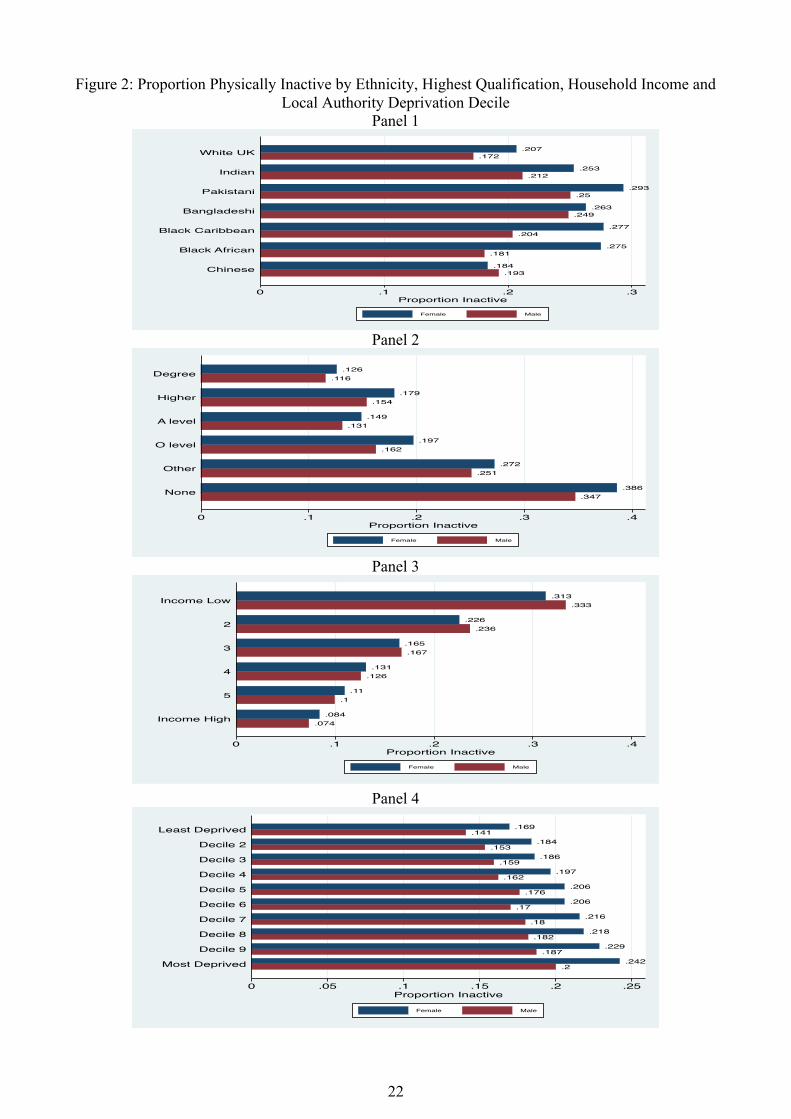
Figure 2 presents patterns of this physical inactivity measure by ethnicity, education,

household income and LA deprivation, for males and females. Panel (1) shows clear differences

across ethnic groups (as well as by gender). With the exception of those of Chinese ethnicity, all

groups are more physically inactive than Whites. The differences are particularly marked for those

of South-East Asian ethnicity (Indian, Pakistani and Bangladeshi). 20 per cent of White females

and 17 per cent of White males had done no physical activity of at least 30 minutes duration in the

four weeks prior to interview. The comparable figures for those of Pakistani ethnicity are nearly 30

and 25 per cent. Differences between males and females vary across ethnic groups: there are

particularly large gaps between males and females of Black African or Caribbean origin, 28 per

cent for men compared to a lower 18 per cent for females. Panel (2) shows the gradient by

education. Degree educated males and females only have a 12 per cent chance of being physically

inactive, whilst those with no qualifications are three times as likely to be physically inactive. Panel

(3) shows these differences are also present by household income: those with lowest income have

more than a 30 per cent chance of doing no physical activity whilst those in the highest group have

a less than a 10 per cent chance. Panel (4) shows these SEP differences are also seen when a

measure of local area deprivation is used. Around 15 per cent of individuals in the least deprived

LA’s do no physical activity; while over 20 per cent of those in the most deprived LA’s do none.

These figures also show that the male-female differential remains controlling for SEP, so that

within SEP category females participate less in sport and recreational physical activity than males.

Figure (3) examines differences by income across age. Panel (1) shows the differences for

males and Panel (2) the differences across females. Lack of physical activity rises, not

unexpectedly, with age. However, for all age groups there is a large difference by income. In the

youngest age group the differences in rates of inactivity between the lowest and highest income

group are approximately two-fold. Nearly 9 per cent of lowest income young males do no activity;

only 4 per cent of highest income young males do none. The comparable figures for females are 15

and 7.5 per cent. Between the age extremes the income gap steadily rises with age, there being

particularly large gaps as individuals approach retirement for both males and females. The relative

differences shrink for the oldest age group so the gap between richest and poorest amongst males

aged 85 or over is only 10 per cent, though for females it is still 20 per cent. However, survivor bias

is likely to narrow this gap at the oldest ages.

We conclude that the raw data shows large SEP differences in physical inactivity. Females,

ethnic minorities, and lower SEP individuals are all less likely to do any activity than males, those

13

classifying themselves as White and those with highest SEP. Income differences also increase with

age.

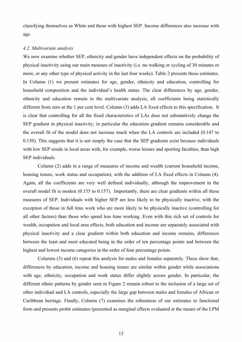
4.2. Multivariate analysis

We now examine whether SEP, ethnicity and gender have independent effects on the probability of

physical inactivity using our main measure of inactivity (i.e. no walking or cycling of 30 minutes or

more, or any other type of physical activity in the last four weeks). Table 2 presents these estimates.

In Column (1) we present estimates for age, gender, ethnicity and education, controlling for

household composition and the individual’s health status. The clear differences by age, gender,

ethnicity and education remain in the multivariate analysis, all coefficients being statistically

different from zero at the 1 per cent level. Column (3) adds LA fixed effects to this specification. It

is clear that controlling for all the fixed characteristics of LAs does not substantively change the

SEP gradient in physical inactivity; in particular the education gradient remains considerable and

the overall fit of the model does not increase much when the LA controls are included (0.147 to

0.150). This suggests that it is not simply the case that the SEP gradients exist because individuals

with low SEP reside in local areas with, for example, worse leisure and sporting faculties, than high

SEP individuals.

Column (2) adds in a range of measures of income and wealth (current household income,

housing tenure, work status and occupation), with the addition of LA fixed effects in Column (4).

Again, all the coefficients are very well defined individually, although the improvement in the

overall model fit is modest (0.155 to 0.157). Importantly, there are clear gradients within all these

measures of SEP. Individuals with higher SEP are less likely to be physically inactive, with the

exception of those in full time work who are more likely to be physically inactive (controlling for

all other factors) than those who spend less time working. Even with this rich set of controls for

wealth, occupation and local area effects, both education and income are separately associated with

physical inactivity and a clear gradient within both education and income remains, differences

between the least and most educated being in the order of ten percentage points and between the

highest and lowest income categories in the order of four percentage points.

Columns (5) and (6) repeat this analysis for males and females separately. These show that,

differences by education, income and housing tenure are similar within gender while associations

with age, ethnicity, occupation and work status differ slightly across gender. In particular, the

different ethnic patterns by gender seen in Figure 2 remain robust to the inclusion of a large set of

other individual and LA controls, especially the large gap between males and females of African or

Caribbean heritage. Finally, Column (7) examines the robustness of our estimates to functional

form and presents probit estimates (presented as marginal effects evaluated at the mean) of the LPM

14

specification in column (4). Comparison of the two columns shows that our estimates are very

robust to functional form and most of the coefficients change very little. Importantly, clear

gradients in all the separate aspects of SEP remain.

In Table 3 we replace the LA fixed effects with observed LA level characteristics that might

be expected to be associated with physical inactivity, including measures of recreational facility

supply and new expenditure, and the local geographical configuration. The model uses the same set

of individual and family level characteristics as the extended models in Table 2, Column 2, but only

the coefficients on the area-level characteristics from this model are presented in the table.

Column (1) Table 3 shows that physical inactivity is significantly related to local-area

deprivation. We extend this analysis in the remaining columns to control for a broader set of local-

area factors that may or may not be correlated with local deprivation. In Column (2) we include

broader regional controls and the degree of urbanization of the LA and in Column (3) we

additionally control for quite detailed characteristics of the LA’s sporting facilities, investment in

new facilities and general satisfaction levels with these facilities and for the weather in the four

week window prior to the respondent’s interview date. Examination of these area level factors

shows that, after controlling for a rich set of both individual and local factors, high-level regional

differences are relatively unimportant, with only the North West and the West Midlands having

higher levels of physical inactivity than the South East. However, there are clear differences at the

LA level and by LA type. The more rural the LA, the less likely the individuals living within it are

to be physically inactive. The greater the number of sports facilities, the higher new expenditure,

and the better the LA facilities satisfaction the less likely individuals are to be physically inactive

(with the exception of sports pitches, which may reflect the presence of professional sports facilities

where individuals watch rather than play). In a cross sectional analysis we cannot separate out

causality (more facilities leads to less inactivity) from selection (individuals who are interested in

physical activity choose to live in places with better facilities) or reverse causation (individuals who

are physically active lobby for better local facilities). Nevertheless it is clear that there is a

statistically significant and sensible association between facilities and lack of inactivity. Finally, the

last block of estimates in column (3) shows that, in England, warm weather promotes overall

physical activity, while rain reduces activity, even after controlling for month of interview.

In Table 4 we test that our results are robust to exactly how physical inactivity is defined.

We replace the measure of inactivity used in Tables 2 and 3 (i.e. no walking or cycling of 30

minutes or more, or any other type of physical activity in the last four weeks) with three specific

measures of physical inactivity that are related to the UK Government targets. As discussed above,

these are based on the number of days in the last four weeks that an individual has participated in

sport or physical recreation for at least 30 minutes with at least moderate intensity. We present

15

estimates for (a) no days (Table 4, Column 1), (b) less than four days (Column 2) and (c) the

inverse of the NI8 measure i.e. less than 12 episodes in the last four weeks (Column 3). We present

only the estimates of the individual measures of SEP that are our focus, but each model controls for

the same extended set of controls and LA fixed effects as Table 2, Column (4).

Age, ethnicity, gender, education and income differences are evident for all three measures.

The differences are similar to those seen for our main physical inactivity measure in Table 2,

indicating that our main measure picks up the public health issues embodied in the national

indicators. Presentation of the national indicator measures also allows comparison of the SEP

gradients as the definition of physical inactivity becomes more absolute. Comparison across the

columns of Table 4 shows that the gradients become steeper as the definition becomes more

absolute. So, for example, the most educated individuals are 15 percentage points less likely to do

no activity but 6 percentage points less likely to not meet the government’s key national indicator

target of 12 episodes of moderate exercise per month than the least educated, while those of Indian

ethnicity are 14 percentage points more likely to do no activity but 7 percentage points less likely to

not meet the key national target than Whites. Differences by income group across the three

measures are also clear.

As we do not have measures of price, the income associations we observe will be picking up

a mixture of an income effect (that individuals who become richer want to do more activity) and a

price effect (that any price will represent a larger share of income for individuals in poorer

households, so will deter activity more in these households). Since price is an important policy

variable we would like to investigate this further. While we cannot control directly for a price

effect, our detailed data means we can examine less costly and more costly activities and so control

indirectly for price. If our income effect is also picking up the price effect then as the activities

become more expensive, the effect of income should become larger. And for the lowest priced

activities we essentially recover the income effect uncontaminated by a direct price effect. In

addition, by looking at less costly and more expensive activities we can separate out the effect of

human capital and knowledge (education) from purchasing power (income). To do this we unpack,

from our main measure of physical inactivity, walking and the three most common activities of

cycling, swimming and using a gym. Walking is least costly and the other activities are more

expensive (though relatively low cost).

Within walking we examine three definitions of lack of walking activity. In Table 5,

Column (1), we present estimates of whether the respondent (1) has not walked continuously for

five minutes in the last month. This is obviously a very marginal measure of physical activity. In

Column (2) we examine whether the respondent has not walked for 30 minutes continuously. In

Column (3) we separate out walking 30 minutes for leisure, which may be more expensive, both in

16

terms of time (as it will take time above any time individuals are paid for) and direct cost, if

individuals travel to do leisure walking. We present only the associations with our key SEP

measures of age, gender, ethnicity, education and income, but our estimates include all other

controls and LA fixed effects.

Column (1) shows that while there are differences by age, gender, ethnicity, and education

in doing no walking at all, these are relatively compressed compared to the differences for the

broader measures of physical inactivity examined in Table 2. Further, there is no income effect.

When we compare doing no walking at all with not undertaking longer amounts of walking

(Column 2), differences by gender, ethnicity and education all widen, suggesting increases in

walking are socially graded. However, not walking for 30 minutes is not strongly associated with

income. But when we examine not walking for leisure we see the association with both education

and income is much stronger for lack of leisure walking than lack of any walking.5 The education

effect therefore seems to be picking up factors such as health knowledge and tastes, while the

income effect probably reflects the effect of the higher price associated with walking for leisure.

To further examine the role of price, we present models of not cycling, not swimming, and

not going to the gym. We separate out not cycling for 30 minutes for any purpose from not cycling

for 30 minutes for leisure alone as the latter may be more expensive than cycling for transport

purposes. Table 6 presents the estimates. Comparison across the columns clearly shows that as the

activity gets more expensive, the association with income rises. Individuals in poorer households

are less likely to do more costly sporting activities. This suggests that price does deter physical

activity. The gradients in education are not patterned by price but are activity specific: there is less

of an education gradient for not cycling than for not undertaking other activities, a little more for

not using the gym, and most for not swimming.

In our final exploration of the role of income we present estimates of the income-age

gradient (more strictly, the income gradient across cohorts). We show in Table 7 estimates of the

linear effect of income and cohort-income interactions but all models also control for the full set of

covariates in Table 2, Column (4). Table 7, Column (1) pools males and females. The first entry in

Column (1) shows the significant effect of income. The coefficient estimate shows that a one-log

point increase in household income is associated with a 1.3 percent points lower probability of

being physically inactive, but that this significantly increases with up to just post-retirement age

(65-74) and falls a little thereafter (75-84). This fall (particularly for 85+ individuals) probably

reflects survivor bias: mortality is patterned by income in the UK, so the lowest income groups in

the oldest cohorts will include more individuals who are in (unobserved) better health. Columns (2) 5 The effect of ethnicity is similar whether we look at any walking in column (2) or leisure walking in column (3), suggesting that lack of walking has a cultural component on top of any other SEP associations. Comparing the effect of age across columns (2) and (3) indicates that individuals in their teens and early 20s do not walk for leisure.

17

and (3) present the estimates for males and females respectively to allow examination of whether

the income gradient differs by gender. While the same increasing income gradient is evident for

both males and females, it is less steep for females. Thus income differences across the physical

inactivity levels of males when young are small, but increase with age substantively, while income

differences in the physical inactivity levels for females exist when young but increase less sharply

across cohorts.

5. Conclusion

In this paper we have exploited an extensive data set to examine physical inactivity in the English

population. Our large sample size allows us to more precisely separate out the various aspects of

SEP that have been conflated in smaller scale studies, to examine different measures of inactivity

and to control for differences at the local level in geography, availability of sporting facilities,

funding for sport and weather.

Our results show several stark facts. The first is the sheer lack of activity: there are very

high levels of physically inactivity in the English population. Around 20 per cent of the population

over the age 16 do minimal levels of physical activity, and about 10 per cent do not even walk

continuously for five minutes over four weeks. The second is that this physical inactivity in

England has a large and robust SEP gradient, however SEP is defined. We show clear evidence of

independent disparities by gender, ethnic group, age, SEP and geographic area in the probability of

being physically inactive. Third, we are able to show that the effect of income is larger for activities

that are more costly while the education gradient is less patterned by cost. Fourth, there is clear

evidence of an income-age gradient. The differences in physical activity by income widen by cohort

with the largest differences occurring in those who are up to 10 years post statutory retirement age.

Finally, we find statistically significant and sensible signs on local area characteristics, but these

explain little of the variance in lack of physical activity.

Our results, coupled with the effect of physical inactivity on later health outcomes, have the

following implications. First, England is building up a large future health problem and one that is

heavily socially graded on a large range of dimensions of SEP. So unless patterns in behaviours are

altered there are likely to be growing SEP disparities in health. Second, our estimates suggest that

all aspects of SEP need to be targeted to influence behavior. The independent effect of income and

its larger effect for more costly activities suggest that price is important, independent of other

aspects of access. This suggests that efforts to lower price barriers might help reduce disparities.

However, it is also clear that education and ethnicity are independent associates of physical

inactivity, so that lowering price barriers will not be enough to tackle these disparities: other more

18

targeted policies are likely to be needed. Finally, the large SEP gaps suggest that the many current

campaigns may not be reaching those who need them most.

References Allender, S., Foster, C., Scarborough, P., Raynor, M. The burden of physical activity-related ill health in the UK. Journal of Epidemiology and Community Health, 2007, 61: 344-348. Allender, S., Foster, C., Boxer, A. Occupational and nonoccupational physical activity and the social determinants of physical activity: Results from the Health Survey for England. Journal of Physical Activity and Health, 2008, 5: 104-116. Arrendondo, E., Mendelson, T., Holub, C., Espinoza, N., Marshall, S. Cultural adaptation of physical activity self-report instruments. Journal of Physical Activity and Health, 2012, 9(S1): S37-S43. Averett, S., Korenman, S. Black-white differences in social and economic consequences of obesity. International Journal of Obesity, 1999, 23(2): 166-173. Baum, C.L., Ford, W.F. The wage effects of obesity: a longitudinal study. Health Economics, 2004, 13(9): 85-899. Borodulin, K., Laatikainen, T., Lahti-Koski, M., Jousilahti, P., Lakka T.A. Association of Age and

education with different types of leisure-time physical activity among 4437 Finnish adults, Journal of Physical Activity and Health, 2008, 5(2): 242-251.

Broderson, N., Steptoe, A., Boniface, D., Wardle, J. Trends in physical activity and sedentary behaviour in adolescence: ethnic and socioeconomic differences. British Journal of Sports Medicine, 2007, 41: 140-144. Bull, F.C. and the Expert Working Groups. Physical Activity Guidelines in the U.K.: Review and

Recommendations. School of Sport, Exercise and Health Sciences, Loughborough University, May 2010.

Bungum, T., Satterwhite, M., Jackson, A., Morrow, J. The relationship of body mass index, medical costs, and absenteeism. American Journal of Health Behavior, 2003, 27(4): 456- 462. Cawley, J., The impact of obesity on wages. Journal of Human Resources, 2004, XXXIX (2): 451- 474. Cleland, V., Ball, K., Magnussen, C., Dwyer, T., Venn, A. Socioeconomic Position and the Tracking of Physical Activity and Cardiorespiratory Fitness From Childhood to Adulthood. American Journal of Epidemiology, 2009, 170: 1069-1077. Cutler, D., Lleras-Muney, A. Education and health: evaluating theories and evidence. NBER Working Paper 12352, June 2006. Das, P., Horton, P. Rethinking our approach to physical activity. The Lancet, 2012, 380: 189-190. de Almeida V., Grace P., Afonso C, et al. Physical activity levels and body weight in a nationally representative sample in the European Union. Public Health Nutrition, 1999, 2: 105–13. Department of Health. Statistics on obesity, physical activity and diet: England 2011. NHS Information Centre, UK, 2011. Dogra, S., Meisner, B.A., Ardern, C. Variation in mode of physical activity by ethnicity and time

since immigration: a cross-sectional analysis. International Journal of Behavioural Nutrition and Physical Activity, 2010, 7(75): doi:10.1186/1479-5868-7-75.

Frost, S., Goins, R.T., Hunter, R., Hooker, S., Bryant, L., Kruger, J., Pluto, D. Effects of the Built Environment on Physical Activity of Adults Living in Rural Settings. American Journal of Health Promotion, 2010, 24: 267-283. Gidlow, C., Johnston, L., Crone, D., Ellis, N., James, D. A systematic review of the relationship

between socio-economic position and physical activity. Health Education Journal, 2006, 65(4): 338–367.

19

Giles-Corti, B., Donovan, R. The relative influence of individual, social and physical environment determinants of physical activity. Social Science & Medicine, 2002, 54(12): 1793-1812. Gomez, J.E., Johnson, B., Selva, M., Sallis, J. Violent crime and outdoor physical activity among

inner-city youth. Preventive Medicine, 2004, 39: 876-881. Greene, W.H., Econometric Analysis Fourth Edition. Prentice Hall International, Inc, 2000. Gregory, J.C., Dhaval, M.D. Physical Activity and Health. National Bureau of Economic Research

Working Paper 18858. Grossman, M. Education and nonmarket outcomes, Chapter 10 in Handbook of the economics of

education. (Eds Hanushek, E., Welch, F.). North-Holland, Netherlands, 2006. Greene, W.H., Econometric Analysis Fourth Edition. Prentice Hall International, Inc, 2000 Hallal, P., Bauman, A., Heath, G., Kohl, H. Physical activity: more of the same is not enough. The

Lancet, 2012, 380: 190-191. Hamer, M., Kivimaki, M., Steptoe, A. Longitudinal patterns in physical activity and sedentary

behaviour from mid-life to early old age: a substudy of the Whitehall II cohort. Journal of Epidemiology and Community Health, forthcoming.

Harrison, R.A., Gemmell, I., Heller, R.F. The population effect of crime and neighborhood on physical activity: an analysis of 15,461 adults. Journal of Epidemiology and Community Health, 2007, 61: 34 –9. Humpel, N., Owen, N., Leslie, E. Environmental factors associated with adults' participation in physical activity. American Journal of Preventive Medicine, 2002, 22: 188-199. Loukaitou-Sideris, A. Is it Safe to Walk? Neighborhood Safety and Security Considerations and

Their Effects on Walking. Journal of Planning Literature, 2006, 20: 219-232. Min Lee, I., Shiroma, E., Lobelo, F., Puska, P., Blair, S., Katzmarzyk, P. Effect of physical

inactivity on major non-communicable diseases worldwide: an analysis of burden of disease and life expectancy. The Lancet, 2012, 380: 219-229.

Moore, L., Diez Roux, A., Evenson, K., McGinn, A., Brines, S. Availability of recreational resources in minority and low socioeconomic status areas. American Journal of Preventive Medicine, 2008, 34: 16-22. Morris, J.N., Heady, J.A., Raffle, P.A., Roberts, C.G., Parks, J.W. Coronary heart-disease and

physical activity of work. Lancet 1953a; 262: 1111–20. Morris, J.N., Heady, J.A., Raffle, P.A., Roberts, C.G., Parks, J.W. Coronary heart-disease and

physical activity of work. Lancet 1953b; 262: 1053–57. Parks, S.E., Housemann, R.A., Brownson, R.C. Differential correlates of physical activity in urban and rural adults of various socioeconomic backgrounds in the United States. Journal of Epidemiology and Community Health, 2003, 57: 29-35. Pascual, C., Regidor, E., Arco, D., Alejos, B., Santos, J., Calle, M., Martinez, D. Sports facilities in

Madrid explain the relationship between neighbourhood economic context and physical inactivity in older people, but not in younger adults: a case study. Journal of Epidemiology and Community Health, 2013, forthcoming.

Philipson, T. The world-wide growth in obesity: an economic research agenda. Health Economics, 2001, 10(1): 1-7. Physical Activity Guidelines Advisory Committee. Physical Activity Guidelines Advisory Committee Report, 2008. Washington, D.C. Powell, L.M., Slater, S., Chaloupka, F.J. The relationship between community physical activity settings and race, ethnicity and socioeconomic status. Evidence Based Preventive Medicine. 2004, 1(2): 135-144. Powell, L., Slater, S., Chaloupka, F., Harper, D. Availability of Physical Activity -related facilities and neighborhood demographic and socioeconomic characteristics: a national study. American Journal of Public Health, 2006, 96: 1676-1680. Saffer, H., Dave, D.M., Grossman, M. Racial, ethnic and gender differences in physical activity. NBER Working Paper 17413, September 2011. Scarborough, P., Bhatnager, P., Wickramasinghe, K., Allender, S., Foster, C., Rayner, M. The

20

economic burden of ill health due to diet, physical inactivity, smoking, alcohol and obesity in the UK: an updateto 2006–07 NHS costs. Journal of Public Health, 2011, 33(4): 527- 535. Sport England. Understanding variations in sports participation. London: Sports England, 2010. Sturm, R. The economics of physical activity. American Journal of Preventive Medicine, 2004, 27(3S): 126-135. Tremblay, M.S., Shephard, R.J., Brawley, L.R., Cameron, C., Craig, C.L., Duggan, M., et al. Physical activity guidelines and guides for Canadians: facts and future. Canadian Journal of Public Health. 2007, 98 (Suppl 2): S218-224. Turrell, G., Haynes, M., Burton, N., Giles-Corti, B., Oldenburg, B., Wilson, L-A., Giskes, K., Brown, W. Neighborhood Disadvantage and Physical Activity: Baseline Results from the HABITAT Multilevel Longitudinal Study. Annals of Epidemiology, 2010, 20: 171-181.US Department of Health and Human Services. Physical activity and health: a report of the Surgeon General. Atlanta, Georgia: US Department of Health and Human Services, Public Health Service, CDC, National Center for Chronic Disease Prevention and Health Promotion, 1996. van Dyck, D., Cardon, G., Deforche, B., Sallis, J., Owen, N., De Bourdeaudhuij, I. Neighborhood SES and walkability are related to physical activity behavior in Belgian adults, Preventive Medicine, 2010, 50: S74. van Lenthe, F.J., Brug, J., Mackenbach, J.P. Neighbourhood inequalities in physical inactivity: the role of neighbourhood attractiveness, proximity to local facilities and safety in the Netherlands. Social Science & Medicine, 2005, 60(4): 763-775. Varo J., Martínez-González M.A, de Irala-Estévez J., Kearney J., Gibney M., Martínez, J. Distribution and determinants of sedentary lifestyles in the European Union. International Journal of Epidemiology, 2003, 32(1): 138–146. Wen, C.P., Wu, X. Stressing harms of physical inactivity to promote exercise. The Lancet, 2012, 380: 192-193. WHO. Reducing risks, promoting healthy life.World Health Report, WHO, Geneva, 2002. WHO. Framework Convention on Tobacco Control. WHO, Geneva, 2003. WHO. Global Strategy on Diet, Physical Activity and Health. Geneva: WHO, Geneva, 2004 WHO. Steps to Health: A European Framework To Promote Physical Activity For Health. WHO: Copenhagen, 2007. Wilbur, J., Chandler, P., Dancy, B. Choi, J., Plonczynski, D. Environmental, policy, and cultural

factors related to physical activity in urban, African American women. Women & Health, 2002, 36(2): 17-28.

Williams, E.D., Stamatakis, E., Chandola, T., Hamer M. Assessment of physical activity levels in South Asians in the UK: findings from the Health Survey for England. Journal of Epidemiology and Community Health, 2011, 65: 517-521.

Figure 1: Relationship between Proportions Inactive (APS) and Obese (HSE) by Local Authority

(Data source: National Obesity Observatory e-atlas; derived from Health Survey for England, 2006-2008)

21

.15.2

.25.3

Prop

ortion

Obe

se

.1 .15 .2 .25 .3Proportion Inactive

22

Figure 2: Proportion Physically Inactive by Ethnicity, Highest Qualification, Household Income and Local Authority Deprivation Decile

Panel 1

Panel 2

Panel 3

Panel 4

.193.184

.181.275

.204.277

.249.263

.25.293

.212.253

.172.207

0 .1 .2 .3Proportion Inactive

Chinese

Black African

Black Caribbean

Bangladeshi

Pakistani

Indian

White UK

Female Male

.347.386

.251.272

.162.197

.131.149

.154.179

.116.126

0 .1 .2 .3 .4Proportion Inactive

None

Other

O level

A level

Higher

Degree

Female Male

.074.084

.1.11

.126.131

.167.165

.236.226

.333.313

0 .1 .2 .3 .4Proportion Inactive

Income High

5

4

3

2

Income Low

Female Male

.2.242

.187.229

.182.218

.18.216

.17.206

.176.206

.162.197

.159.186

.153.184

.141.169

0 .05 .1 .15 .2 .25Proportion Inactive

Most Deprived

Decile 9

Decile 8

Decile 7

Decile 6

Decile 5

Decile 4

Decile 3

Decile 2

Least Deprived

Female Male

23

Figure 3: Proportion Physically Inactive by Age and High/Low Household Income (Top Panel = Males; Bottom Panel = Females)

Panel 1

Panel 2

.421.622

.378.479

.139.34

.105.307

.095.295

.078.219

.07.186

.074.147

0 .2 .4 .6Proportion Inactive

85+

75-84

65-74

55-64

45-54

35-44

25-34

16-24

Low Income High Income

.499.603

.299.472

.127.371

.109.361

.084.326

.067.261

.052.188

.036.088

0 .2 .4 .6Proportion Inactive

85+

75-84

65-74

55-64

45-54

35-44

25-34

16-24

Low Income High Income

24

Table 1: Sample Characteristics: Covariates and Physical Inactivity Measures Covariates Mean SD Covariates Mean SD Age 16-24 0.079 0.269 Working full-time 0.406 0.491 Age 25-34 0.128 0.334 Working part-time 0.153 0.360 Age 35-44 0.193 0.394 Unemployed<12 months 0.020 0.140 Age 45-54 0.177 0.381 Unemployed>12 months 0.025 0.155 Age 55-64 0.189 0.391 Retired 0.282 0.450 Age 65-74 0.141 0.348 Non-participant (home/child) 0.047 0.212 Age 75-84 0.079 0.270 Non-participant (disabled) 0.024 0.154 Age 85 or above 0.017 0.128 Student 0.038 0.190 Male 0.411 0.492 Other 0.005 0.076 UK White 0.896 0.305 North East 0.063 0.242 Indian 0.014 0.117 North West 0.129 0.336 Pakistani 0.007 0.085 Yorkshire 0.058 0.234 Bangladeshi 0.002 0.044 West Midlands 0.106 0.308 Caribbean 0.010 0.097 East Midlands 0.112 0.316 African 0.009 0.097 East 0.133 0.339 Chinese 0.002 0.046 South West 0.121 0.326 Other ethnic groups 0.060 0.046 South East 0.183 0.387 Single adult 0.366 0.482 London 0.095 0.293 Child aged 0-4 0.102 0.303 Urban 1 (Most urban) 0.236 0.425 Child aged 5-10 0.141 0.348 Urban 2 0.126 0.332 Child aged 11-15 0.128 0.334 Urban 3 0.149 0.357 Log household Size 0.689 0.554 Urban 4 0.142 0.349 Chronic limiting condition 0.179 0.383 Urban 5 0.157 0.364 Cannot walk 0.015 0.123 Urban 6 (Most Rural) 0.189 0.392 Degree of higher education 0.307 0.461 Log (% Green Space) 4.183 0.441 Higher education (less than degree) 0.100 0.301 IMD Deprivation Index 19.689 9.302 ‘A’ levels 0.158 0.364 Log (Unemployment Rate) 1.664 0.325 ‘O’ level 0.237 0.430 Log (Percentage Non-UK British) 1.952 0.801 Other 0.035 0.184 Log (Main Pools per 10,000 pop) -0.772 0.590 No qualifications 0.164 0.370 Log (Health Suites per 10,000) 0.092 0.490 Income: £52,000 or more 0.158 0.364 Log (Sports Halls per 10,000 ) 0.500 0.481 £41,600 to £51,999 0.101 0.301 Log (Sports Pitches per 10,000) 1.795 0.702 £31,200 to £41,599 0.140 0.347 Log (Lottery Amount per 10,000) 11.659 1.420 £20,800 to £31,199 0.201 0.401 Log (LA Facilities Satisfaction) 1.306 0.038 £10,400 to £20,700 0.250 0.433 Mean Precipitation 2.079 1.299 <£10,400 per annum 0.150 0.357 Maximum Temperature 14.137 5.816 Council or LA housing 0.124 0.330 Minimum Temperature Squared/10 233.662 167.795 Occ class: Higher managerial 0.058 0.235 Higher professional 0.084 0.277 Physical Inactivity Measures Mean SD Lower professional 0.195 0.396 Physically Inactive (Main measure) 0.197 0.398 Lower managerial 0.079 0.270 KPV=0 0.506 0.500 Higher supervisor 0.053 0.224 KPV<4 0.592 0.491 Intermediate 0.114 0.317 KPV<12 0.792 0.406 Employer 0.025 0.156 No Walk 5 Minutes 0.096 0.295 Own account worker 0.083 0.276 No Walk 30 Minutes (All) 0.295 0.456 Lower supervisor 0.079 0.269 No Walk 30 Minutes (Leisure) 0.464 0.499 Lower technical 0.022 0.147 No Cycling 30 Minutes (All) 0.894 0.308 Semi-routine 0.124 0.329 No Cycling 30 Minutes (Leisure) 0.913 0.281 Routine 0.068 0.251 No Swimming 0.875 0.330 Unknown 0.017 0.129 No Gym 0.903 0.296 Notes: Raw sample means and standard deviations shown. Mean values calculated conditional on no missing observations. Mean value for occupational classifications are conditional on respondent reporting to work either full-time or part-time.

25

Table 2: Linear Probability and Binary Probit Models of Physical Inactivity (1= Physically Inactive in last 4 weeks; 0 = otherwise)

Linear Probability Models Probit Without LA Fixed Effects With LA Fixed Effects

(1) All

(2) All

(3) All

(4) All

(5) Males

(6) Females

(7) All

! t-stat ! t-stat ! t-stat ! t-stat ! t-stat ! t-stat

ME

z-stat Age 25-34 0.038 19.12 0.029 13.12 0.038 19.53 0.029 13.09 0.043 13.00 0.014 4.42 0.039 12.72 Age 35-44 0.053 28.75 0.046 20.56 0.053 29.10 0.046 20.52 0.063 18.08 0.026 8.45 0.064 20.48 Age 45-54 0.073 34.26 0.065 29.91 0.074 33.13 0.065 29.35 0.086 26.28 0.041 14.31 0.092 31.45 Age 55-64 0.090 38.45 0.090 33.05 0.092 37.45 0.091 32.57 0.120 32.30 0.058 15.92 0.126 33.85 Age 65-74 0.119 47.75 0.139 42.70 0.121 47.96 0.141 42.59 0.157 36.15 0.117 24.58 0.189 43.05 Age 75-84 0.238 78.89 0.263 69.73 0.241 78.58 0.265 69.31 0.269 49.79 0.253 50.94 0.326 61.74 Age 85 or above 0.392 70.48 0.419 68.52 0.397 73.61 0.424 70.16 0.431 50.50 0.408 51.26 0.507 67.38 Male -0.014 -12.18 -0.019 -16.14 -0.014 -12.56 -0.020 -16.49 - - - - -0.021 -17.15 Indian 0.119 25.67 0.114 24.15 0.106 22.39 0.103 21.38 0.097 17.49 0.110 14.39 0.132 23.51 Pakistani 0.155 22.75 0.147 21.98 0.143 17.59 0.136 17.11 0.126 9.55 0.145 19.87 0.170 20.14 Bangladeshi 0.153 11.63 0.136 9.39 0.151 12.55 0.137 11.46 0.142 8.10 0.130 8.43 0.181 14.71 Caribbean 0.089 12.14 0.076 10.59 0.081 11.14 0.070 10.16 0.038 3.70 0.097 11.37 0.085 12.20 African 0.126 18.55 0.109 15.59 0.119 18.76 0.105 16.63 0.071 9.39 0.138 13.58 0.139 21.25 Chinese 0.100 7.79 0.100 7.96 0.101 8.17 0.101 8.40 0.115 6.18 0.089 6.53 0.143 10.05 Other ethnic groups 0.033 11.52 0.029 10.60 0.034 14.88 0.031 13.81 0.028 9.03 0.034 11.30 0.041 15.58 Single adult 0.024 11.49 0.012 5.30 0.022 10.94 0.010 4.81 0.016 4.70 0.006 1.97 0.010 4.65 Child aged 0-4 0.014 6.71 0.015 7.38 0.014 6.68 0.015 7.24 0.011 3.85 0.015 5.09 0.018 7.14 Child aged 5-10 -0.014 -8.63 -0.012 -7.57 -0.014 -8.70 -0.012 -7.73 -0.012 -4.45 -0.012 -5.93 -0.014 -7.29 Child aged 11-15 -0.013 -7.05 -0.011 -5.75 -0.013 -7.05 -0.011 -5.86 -0.012 -4.92 -0.010 -3.87 -0.013 -5.69 Log household Size 0.008 3.65 0.010 4.62 0.007 3.16 0.009 3.91 0.006 2.10 0.013 3.88 0.011 4.26 Chronic limiting condition 0.175 76.61 0.155 72.83 0.173 79.36 0.154 73.89 0.153 48.00 0.155 63.88 0.144 83.90 Cannot walk 0.450 113.21 0.429 103.77 0.449 112.02 0.428 103.24 0.432 57.85 0.424 89.35 0.482 75.24 Degree of higher education -0.140 -70.49 -0.110 -55.76 -0.133 -69.50 -0.104 -54.25 -0.098 -35.13 -0.109 -41.39 -0.084 -50.09 Higher education (less than degree) -0.109 -49.71 -0.089 -40.52 -0.104 -49.21 -0.085 -39.82 -0.077 -24.72 -0.092 -32.79 -0.060 -33.37 ‘A’ levels -0.099 -46.06 -0.082 -39.27 -0.095 -45.35 -0.080 -38.43 -0.073 -24.38 -0.087 -30.04 -0.058 -32.76 ‘O’ level -0.072 -39.93 -0.063 -34.64 -0.070 -39.37 -0.061 -34.02 -0.058 -22.01 -0.063 -24.52 -0.041 -27.79 Other -0.069 -21.60 -0.059 -18.62 -0.066 -20.44 -0.057 -17.72 -0.052 -11.40 -0.065 -13.67 -0.038 -14.84 Income: £52,000 or more - - -0.042 -8.30 - - -0.039 -7.66 -0.045 -5.50 -0.033 -5.72 -0.042 -7.64 £41,600 to £51,999 - - -0.030 -5.67 - - -0.028 -5.30 -0.032 -3.66 -0.027 -4.02 -0.027 -4.83 £31,200 to £41,599 - - -0.018 -3.89 - - -0.017 -3.67 -0.023 -2.85 -0.015 -2.63 -0.013 -2.91 £20,800 to £31,199 - - -0.014 -2.97 - - -0.013 -2.74 -0.018 -2.36 -0.012 -2.16 -0.008 -1.78 £10,400 to £20,700 - - -0.008 -1.80 - - -0.007 -1.56 -0.010 -1.29 -0.006 -1.15 -0.002 -0.39

26

Council or LA housing - - 0.036 17.81 - - 0.037 18.94 0.036 11.67 0.038 16.39 0.035 19.00 Table 2: (Continued)

Occ class: Higher managerial - - -0.040 -12.85 - - -0.038 -12.16 -0.049 -11.59 -0.017 -3.43 -0.043 -13.09 Higher professional - - -0.041 -12.18 - - -0.038 -11.42 -0.044 -10.30 -0.030 -6.16 -0.044 -12.45 Lower professional - - -0.041 -12.65 - - -0.040 -12.37 -0.054 -12.70 -0.017 -4.07 -0.046 -14.34 Lower managerial - - -0.025 -7.36 - - -0.023 -6.90 -0.038 -8.66 0.005 1.07 -0.023 -7.01 Higher supervisor - - -0.039 -11.45 - - -0.038 -11.42 -0.061 -13.88 -0.005 -0.98 -0.040 -11.62 Intermediate - - -0.012 -3.59 - - -0.013 -3.77 -0.032 -6.98 0.010 2.45 -0.013 -3.94 Employer - - -0.019 -4.31 - - -0.015 -3.53 -0.024 -4.37 0.003 0.34 -0.013 -2.97 Own account worker - - -0.024 -6.24 - - -0.021 -5.39 -0.021 -4.16 -0.028 -5.77 -0.021 -5.53 Lower supervisor - - -0.032 -8.68 - - -0.031 -8.42 -0.041 -9.29 -0.009 -1.83 -0.031 -8.62 Lower technical - - -0.009 -1.98 - - -0.008 -1.80 -0.013 -2.64 -0.008 -0.62 -0.008 -1.71 Semi-routine - - -0.017 -4.61 - - -0.016 -4.51 -0.020 -3.69 -0.001 -0.27 -0.016 -4.64 Unknown - - -0.029 -5.10 - - -0.028 -4.85 -0.038 -5.25 -0.008 -1.01 -0.030 -4.92 Working part-time - - -0.042 -28.51 - - -0.040 -26.98 -0.042 -13.67 -0.035 -19.58 -0.042 -24.93 Unemployed<12 months - - -0.051 -10.73 - - -0.050 -10.56 -0.058 -9.05 -0.031 -5.62 -0.049 -10.53 Unemployed>12 months - - -0.024 -5.01 - - -0.023 -5.00 -0.028 -4.44 -0.008 -1.26 -0.025 -6.00 Retired - - -0.067 -21.06 - - -0.066 -20.79 -0.074 -15.50 -0.041 -9.47 -0.065 -22.80 Non-participant (home/child) - - -0.055 -15.31 - - -0.052 -14.45 -0.045 -3.53 -0.035 -7.47 -0.050 -15.49 Non-participant (disabled) - - 0.091 16.31 - - 0.091 16.36 0.083 11.08 0.110 15.64 0.048 10.32 Student - - -0.070 -17.13 - - -0.068 -16.41 -0.076 -15.00 -0.053 -10.14 -0.073 -15.64 Other - - -0.046 -6.81 - - -0.044 -6.53 -0.051 -3.88 -0.025 -2.67 -0.045 -7.61 LA Fixed Effects (326) NO NO NO NO YES YES YES YES YES YES YES YES YES YES (Pseudo) R-squared 0.147 0.155 0.150 0.157 0.153 0.161 0.145 Sample 1,002,216 1,002,216 1,002,216 1,002,216 411,828 590,388 1,002,216

Notes: Coefficients from linear probability models, and marginal effects (evaluated at X-bar) from binary probit model, and associated t-statistics (z), shown. Omitted categories are aged 16-24, female, White British, more than one adult in household, no children under 16, no chronic limiting health condition, can walk, no qualifications, annual household income less than £10,400, working full-time, does not reside (rent) in a council or housing association house, works in a ‘routine’ occupation, works full-time, lives in a major urban area, and lives in the South East. Each model additionally controls for month of interview, survey year, as well dummy variables for missing information. LA national proportion weights applied. Household income bands * linear time trends included in each model that controls for household income. Robust standard errors clustered by (326) local authority.

27

Table 3: Linear Probability Models of Physical Inactivity with Observable LA Characteristics

Controlling for LA Observables (1) (2) (3) ! t-stat ! t-stat ! t-stat

LA Deprivation Index (Decile 2) 0.002 0.57 0.002 0.50 0.001 0.20 LA Deprivation Index (Decile 3) 0.003 1.08 0.002 0.69 0.001 0.35 LA Deprivation Index (Decile 4) 0.005 1.48 0.005 1.31 0.002 0.45 LA Deprivation Index (Decile 5) 0.012 2.64 0.009 1.99 0.005 1.24 LA Deprivation Index (Decile 6) 0.011 2.37 0.009 1.74 0.004 0.89 LA Deprivation Index (Decile 7) 0.014 3.30 0.013 3.17 0.008 2.00 LA Deprivation Index (Decile 8) 0.018 4.46 0.015 2.75 0.010 1.81 LA Deprivation Index (Decile 9) 0.020 5.58 0.014 3.00 0.011 2.15 LA Deprivation Index (Decile 10; most deprived) 0.027 6.07 0.022 3.89 0.018 3.28 North East - - 0.009 1.62 0.013 2.46 North West - - 0.006 1.40 0.008 2.04 Yorkshire - - 0.001 0.17 0.001 0.28 West Midlands - - 0.016 4.11 0.014 3.99 East Midlands - - 0.007 1.89 0.005 1.41 East - - 0.011 2.79 0.009 2.44 London - - 0.001 0.14 0.003 0.49 South West - - -0.008 -2.02 -0.007 -1.85 Urban 2 (More Urban) - - -0.008 -2.56 -0.008 -2.55 Urban 3 - - -0.010 -2.60 -0.006 -1.68 Urban 4 - - -0.015 -3.49 -0.011 -2.40 Urban 5 - - -0.016 -3.67 -0.014 -3.29 Urban 6 (More Rural) - - -0.022 -4.84 -0.021 -4.40 Log (% Green Space) - - 0.013 2.70 -0.002 -0.50 Log (Percentage Non-UK British) - - 0.001 0.56 0.002 1.03 Log (Main Pools per 10,000 pop) - - - - -0.006 -1.75 Log (Health Suites per 10,000) - - - - -0.010 -2.21 Log (Sports Halls per 10,000) - - - - -0.002 -0.41 Log (Sports Pitches per 10,000) - - - - 0.014 4.83 Log (Lottery Amount per 10,000) - - - - -0.001 -1.13 Log (LA Facilities Satisfaction) - - - - -0.059 -1.92 Mean Precipitation - - - - 0.001 1.56 Maximum Temperature - - - - -0.005 -6.87 Maximum Temperature Squared / 10 - - - - 0.001 4.78 LA Fixed Effects (326) NO NO NO NO NO NO (Pseudo) R-squared 0.155 0.155 0.156 Sample 1,002,216 1,002,216 1,001,203 Notes: Selected coefficients on LA observable characteristics from linear probability models, and associated t-statistics (z), shown. Omitted categories are LA Deprivation Index Decile 1 (least deprived), South East and Major Urban. Each model has the same controls as Table 2, Column 2. Respondents from two local authorities: City of London, and Isles of Scilly, are dropped from the last model due to missing data (these are the two smallest LAs by population in England).

28

Table 4: Linear Probability Models of National Indicator Based Measures of Physical Inactivity KPV=0 KPV<4 KPV<12 (1) (2) (3) ! t-stat ! t-stat ! t-stat

Age 25-34 0.072 21.90 0.068 19.61 0.047 14.19 Age 35-44 0.122 39.96 0.119 35.88 0.083 28.74 Age 45-54 0.189 59.89 0.179 53.40 0.125 44.26 Age 55-64 0.255 79.16 0.234 68.99 0.168 53.41 Age 65-74 0.328 84.15 0.297 76.00 0.208 60.14 Age 75-84 0.455 98.31 0.404 89.77 0.269 70.19 Age 85 or above 0.539 98.80 0.475 90.87 0.301 73.01 Male -0.070 -40.54 -0.062 -33.50 -0.043 -27.79 Indian 0.144 21.74 0.120 18.08 0.066 13.41 Pakistani 0.165 15.64 0.145 16.08 0.080 11.32 Bangladeshi 0.185 9.96 0.152 9.14 0.101 11.92 Caribbean 0.062 8.45 0.065 10.51 0.027 4.84 African 0.163 23.66 0.140 21.74 0.089 16.12 Chinese 0.125 7.70 0.133 7.63 0.103 7.84 Other ethnic groups 0.046 16.11 0.038 13.35 0.021 8.97 Chronic limiting condition 0.134 63.48 0.124 63.74 0.068 46.81 Cannot walk 0.101 29.71 0.078 24.05 0.039 20.79 Degree of higher education -0.154 -66.27 -0.131 -59.95 -0.064 -35.58 Higher education (less than degree) -0.120 -40.40 -0.099 -33.70 -0.051 -21.66 ‘A’ levels -0.114 -48.49 -0.097 -42.66 -0.049 -24.71 ‘O’ level -0.075 -35.70 -0.062 -28.91 -0.024 -13.64 Other -0.067 -19.94 -0.050 -14.90 -0.018 -7.35 Income: £52,000 or more -0.156 -26.51 -0.169 -27.14 -0.126 -21.81 £41,600 to £51,999 -0.117 -19.54 -0.120 -19.43 -0.074 -12.16 £31,200 to £41,599 -0.093 -14.27 -0.095 -14.14 -0.056 -11.31 £20,800 to £31,199 -0.068 -12.84 -0.066 -12.37 -0.032 -7.95 £10,400 to £20,700 -0.017 -3.62 -0.021 -4.73 -0.008 -2.03 Council or LA housing 0.067 29.21 0.059 25.63 0.032 19.68 LA Fixed Effects (326) YES YES YES YES YES YES R-squared 0.196 0.152 0.078 Sample 993,096 993,096 993,096 Notes: Selected coefficients from linear probability models with LA fixed effects, and associated t-statistics, shown. Each model has the same controls as Table 2, Column 4.

29

Table 5: Linear Probability Models of Walking-Related Inactivity

No Walk 5

No Walk 30

All No Walk 30

Leisure ! t-stat ! t-stat ! t-stat

Age 25-34 0.009 5.45 0.003 0.88 -0.087 -21.81 Age 35-44 0.008 4.68 0.005 1.35 -0.128 -30.35 Age 45-54 0.010 5.72 0.006 2.11 -0.148 -35.42 Age 55-64 0.014 7.06 0.020 6.05 -0.145 -32.97 Age 65-74 0.035 13.86 0.079 19.06 -0.088 -21.21 Age 75-84 0.090 29.09 0.207 46.06 0.045 8.47 Age 85 or above 0.191 37.86 0.357 55.20 0.175 25.60 Male 0.009 10.43 0.019 14.31 0.029 17.76 Indian 0.044 12.66 0.162 29.00 0.151 25.28 Pakistani 0.045 11.32 0.180 19.40 0.162 13.70 Bangladeshi 0.045 8.50 0.161 13.08 0.160 11.12 Caribbean 0.027 8.37 0.142 20.10 0.146 18.39 African 0.068 17.86 0.170 24.43 0.174 28.34 Chinese 0.084 9.74 0.169 11.71 0.191 12.32 Other ethnic groups 0.026 16.30 0.042 14.14 0.046 14.38 Chronic limiting condition 0.087 54.99 0.159 79.32 0.127 50.13 Cannot walk - - - - - - Degree of higher education -0.051 -30.41 -0.106 -46.62 -0.150 -63.00 Higher education (less than degree) -0.043 -21.73 -0.077 -28.10 -0.116 -36.21 ‘A’ levels -0.041 -23.80 -0.073 -31.12 -0.106 -41.59 ‘O’ level -0.035 -20.67 -0.052 -23.07 -0.068 -28.33 Other -0.027 -9.74 -0.043 -11.25 -0.072 -19.18 Income: £52,000 or more 0.001 0.21 0.001 0.13 -0.041 -6.02 £41,600 to £51,999 0.000 -0.08 0.008 1.19 -0.025 -3.49 £31,200 to £41,599 0.000 0.11 0.014 2.52 -0.014 -2.24 £20,800 to £31,199 -0.002 -0.51 0.007 1.20 -0.011 -1.67 £10,400 to £20,700 -0.004 -1.24 0.001 0.28 -0.003 -0.53 Council or LA housing 0.012 8.25 0.025 9.22 0.062 23.32 LA Fixed Effects (326) YES YES YES YES YES YES R-squared 0.055 0.080 0.090 Sample 986,863 986,863 983,286 Notes: Selected coefficients from linear probability models with LA fixed effects, and associated t-statistics, shown. Each model has the same controls as Table 2, Column 4. Individuals reporting that they cannot walk are dropped from the estimation sample.

30

Table 6: Linear Probability Models of Cycling, Swimming and Gym Inactivity

No Cycling 30

All No Cycling 30

Leisure No Swimming No Gym ! t-stat ! t-stat ! t-stat ! t-stat

Age 25-34 0.029 13.04 0.016 7.68 0.015 6.25 0.023 7.88 Age 35-44 0.024 10.65 0.008 4.29 0.012 5.24 0.060 19.68 Age 45-54 0.053 22.88 0.033 16.66 0.030 12.18 0.094 34.86 Age 55-64 0.085 36.71 0.060 29.73 0.047 19.17 0.118 43.44 Age 65-74 0.112 44.98 0.083 38.06 0.067 26.59 0.135 43.59 Age 75-84 0.136 49.81 0.104 42.95 0.103 38.15 0.158 49.83 Age 85 or above 0.145 47.11 0.110 43.13 0.122 40.30 0.166 48.57 Male -0.076 -68.61 -0.057 -52.66 0.061 45.65 0.003 2.78 Indian 0.089 23.74 0.067 21.45 0.069 20.95 -0.004 -0.81 Pakistani 0.088 18.48 0.069 16.77 0.094 25.73 -0.003 -0.36 Bangladeshi 0.094 11.77 0.066 8.31 0.086 14.49 0.005 0.61 Caribbean 0.034 5.59 0.024 6.25 0.073 24.00 -0.026 -4.88 African 0.081 16.13 0.062 23.32 0.100 33.05 0.009 1.72 Chinese 0.051 3.67 0.042 3.24 0.024 2.23 0.031 3.06 Other ethnic groups 0.015 5.87 0.015 7.28 0.028 14.61 -0.005 -2.64 Chronic limiting condition 0.027 24.37 0.021 21.41 0.014 10.69 0.023 21.15 Cannot walk 0.017 12.31 0.013 11.81 0.014 7.06 0.007 4.62 Degree of higher education -0.021 -14.75 -0.020 -17.24 -0.059 -38.04 -0.037 -25.51 Higher education (less than degree) -0.013 -7.93 -0.017 -10.50 -0.041 -21.82 -0.023 -12.79 ‘A’ levels -0.001 -0.40 -0.007 -4.86 -0.040 -26.24 -0.028 -17.83 ‘O’ level 0.000 -0.17 -0.002 -1.74 -0.017 -13.98 -0.010 -7.48 Other 0.003 1.35 -0.001 -0.71 -0.024 -11.67 -0.012 -6.13 Income: £52,000 or more -0.020 -4.44 -0.031 -7.96 -0.037 -7.11 -0.094 -19.00 £41,600 to £51,999 0.003 0.48 -0.009 -1.81 -0.033 -7.83 -0.056 -10.98 £31,200 to £41,599 -0.007 -1.51 -0.011 -2.68 -0.031 -7.46 -0.041 -9.81 £20,800 to £31,199 -0.005 -1.43 -0.010 -3.27 -0.018 -4.61 -0.019 -5.74 £10,400 to £20,700 0.004 1.28 0.002 0.85 -0.011 -3.39 -0.004 -1.40 Council or LA housing 0.014 8.17 0.014 9.71 0.017 13.79 0.020 15.60 LA Fixed Effects (326) YES YES YES YES R-squared 0.071 0.057 0.043 0.056 Sample 1,002,216 1,002,015 1,002,039 1,002,113

Notes: Selected coefficients from linear probability models with LA fixed effects, and associated t-statistics, shown. Each model has the same controls as Table 2, Column 4.

31

Table 7: Interactions of Age and Household Income in Linear Models of Physical Inactivity

All Males Females ! t-stat ! t-stat ! t-stat

Log (HH Income) -0.013 -5.02 -0.005 -1.38 -0.017 -4.06 (Age 25-34) * (Log (HH Income)) -0.009 -2.67 -0.020 -4.21 -0.002 -0.49 (Age 35-44) * (Log (HH Income)) -0.016 -4.63 -0.028 -5.53 -0.010 -2.04 (Age 45-54) * (Log (HH Income)) -0.026 -6.83 -0.042 -8.27 -0.017 -3.58 (Age 55-64) * (Log (HH Income)) -0.027 -8.18 -0.044 -10.04 -0.023 -4.39 (Age 65-74) * (Log (HH Income)) -0.046 -11.80 -0.068 -11.62 -0.034 -6.00 (Age 75-84) * (Log (HH Income)) -0.036 -7.25 -0.050 -6.68 -0.025 -3.37 (Age 85+) * (Log (HH Income)) 0.004 0.42 -0.006 -0.41 0.008 0.48 LA Fixed Effects (326) YES YES YES YES YES YES Sample 745,997 327,811 418,186

Notes: Selected coefficients from linear probability for log household income, and interactions between age dummies and log household income shown. Each model has the same controls as Table 2, Column 4. Cases with missing household income are dropped from the estimation sample.