the cbc system for choice-based conjoint · pdf filethe cbc system for choice-based conjoint...

1

© Copyright 1993-2017, Sawtooth Software, Inc.

1457 E 840 N Orem, Utah

+1 801 477 4700

www.sawtoothsoftware.com

Sawtooth Software

TECHNICAL PAPER SERIES

The CBC System for

Choice-Based Conjoint Analysis

Version 9

Sawtooth Software, Inc.

2

The CBC System for Choice-Based Conjoint Analysis

Copyright Sawtooth Software, Inc.

Orem, Utah USA

(801) 477-4700

August, 2017

The CBC System is a component within Sawtooth Software’s Lighthouse Studio platform for

conducting “choice-based” conjoint analysis studies, also known as stated choice experiments.

The CBC software may be used in web-based data collection, using devices not connected to the

web (CAPI mode), or with paper-and-pencil studies. The main characteristic distinguishing

choice-based conjoint analysis from other types is that the respondent expresses preferences by

choosing concepts from sets of concepts, rather than by rating or ranking them.

Although it had been discussed by academics for many years (Louviere and Woodworth, 1983),

most large-scale commercial use of choice-based conjoint started to occur in the 1990s with the

first version of CBC software released by Sawtooth Software in 1993. According to surveys of

Sawtooth Software customers, we believe CBC became the most widely used conjoint-related

method in about 2000. Today, it is clear that CBC is the most widely used flavor of conjoint

analysis.

This paper discusses the method of choice-based conjoint analysis from a practitioner-oriented

point of view and describes Sawtooth Software's CBC System for choice-based conjoint analysis

in some detail. It also provides suggestions about how to select a particular conjoint method

from the variety of those available, considering characteristics of the research problem at hand.

The Role of Choice-Based Conjoint Analysis

Choice-based conjoint analysis has attracted much interest in the marketing research field. There

are several reasons for its position as the most widely used conjoint-related approach today:

The task of choosing a preferred concept is similar to what buyers actually do in the

marketplace. Choosing a preferred product from a group of products is a simple and

natural task that everyone can understand.

Choice-based conjoint analysis lets the researcher include a "None" option for

respondents, which might read "I wouldn't choose any of these." By selecting that option,

a respondent can contribute information about the decrease in demand to be expected if,

for example, prices of all offered products increased or the products became unattractive

in other ways.

Most conjoint analysis studies use "main effects only" assumptions. However,

choice-based conjoint analysis experiments may be made efficient enough to quantify

interactions.

3

It is possible in choice-based conjoint analysis to have "product- or alternative-specific"

attribute levels. For example, in studying transportation we might consider walking shoes

and bicycles. The attributes describing shoes are different from those describing bicycles,

and yet one might want to study both kinds of products at the same time to learn how

much improvement in walking shoes would be required to switch a respondent from

cycling to walking. Specifying alternative-specific attributes is available in the CBC

Advanced Design Module (an add-on component).

With the use of hierarchical Bayesian (HB) estimation (integrated within the CBC

system), part-worth utilities at the individual-level may be estimated. This development

occurred in the mid-1990s, and has greatly improved the usability and predictive validity

of CBC data.

However, choice-based conjoint analysis does have disadvantages, due to the fact that having

respondents make choices is an inefficient way to elicit preferences. Each concept is typically

described on all the attributes being considered in the study, and each choice set contains several

concepts. Therefore, the respondent is being asked to process a lot of information before giving a

single answer for each choice set. Although this does mimic what happens in the marketplace,

the analyst ends up with far less information than would have been available had the task been to

rate each alternative in the set. For that reason, in the 1980s through most of the 1990s, choice-

based conjoint studies were not used for estimating the values that individual respondents

attached to attribute levels, as had been commonplace with traditional conjoint methods. Instead,

data from groups of respondents were typically aggregated for analysis. This was done either by

combining all respondents or by studying subsets defined by specific market segments. “Utility

values” would be produced for each group of respondents that summarized the choices made by

those individuals. And, as in other conjoint methods, the utility values could be used to simulate

and predict market reactions to product concepts that may not have actually appeared in the

choice tasks (questions).

Aggregation and group-based analysis had strong disadvantages, and this delayed the acceptance

of CBC analysis throughout the 1980s and early 1990s. Aggregating respondents in CBC

analysis assumes respondent homogeneity, which may not always be appropriate or desirable.

Later developments in the 1990s recognized segment-based or even respondent-by-respondent

differences. Latent Class analysis (integrated within the CBC system) can simultaneously

discover relatively homogeneous segments and estimate their preference functions. In the late

1990s, computationally intensive Bayesian estimation for CBC became relatively commonplace

and it permitted estimating individual-level utilities from choice data. Latent Class and HB

generally lead to more accurate predictions than the methods of pure aggregation.

Full-profile choice-based conjoint analysis is generally not appropriate for studies involving large

numbers of attributes. Each task presents concepts that are described on all the attributes, and

there is a limit to how much information respondents can process without becoming confused or

4

overloaded. Green and Srinivasan (1990) suggested about six as the maximum number of

attributes to handle with full-profile concepts in traditional conjoint analysis. There has been a

great deal of debate regarding this recommendation. Most leading researchers in conjoint

analysis now believe that if the attributes are written succinctly (especially if graphics are used)

and the information is laid out well on the screen, respondents can probably evaluate more than

six attributes at a time in CBC. The reality is that many respondents end up ignoring

unimportant attributes and using shortcut heuristics to select the winning concept. This behavior

might be realistic and observed in real world choices, but the researcher should be mindful that

increasing the number of attributes in CBC interviews increases the likelihood that respondents

will simplify the task. The base CBC system permits a maximum of ten attributes with at most

15 levels per attribute. The Advanced Design Module add-on permits up to 100 attributes (each

with up to 254 levels) and supports partial-profile format, where only a subset of the attributes is

presented in each question.

One of the strengths of CBC is its ability to deal with interactions. Most conjoint methods are

based on “main effects only” models that ignore the existence of interactions. CBC, in contrast,

can measure two-way interactions. Interactions occur when the net utility effect of levels from

two separate attributes is significantly more or less than what would be predicted by summing

their main effect parts. For example, chocolate is good. Cheese is good. But, chocolate-covered

cheese is not good. We think that CBC provides a good way to produce relatively precise results

when there are few attributes and their interactions are of concern. The ability to investigate

interactions is enhanced by questionnaires that permit some “level overlap,” which we discuss

later in this paper.

The concern for interactions is typical of many pricing studies. It can be demonstrated that

interaction effects can be revealed through market simulations by disaggregate main-effect

models that do not directly model interaction terms, if the source of the interactions between

attributes is principally due to differences in preference between groups or individuals.

Therefore, if Latent Class or hierarchical Bayes is used to model main-effects, the need to

additionally model interactions may be lessened. Either way, the questionnaire designs offered in

CBC are appropriate for aggregate or disaggregate analysis; for main-effects or models that

involve interactions. We recommend that researchers be on the lookout for significant

interaction effects even if using HB estimation (Sawtooth Software’s CBC/HB Model Explorer is

a recent and suggested tool for investigating valuable interaction effects).

To summarize our position briefly, full-profile choice-based conjoint analysis provides a good

way to produce relatively precise results when there are relatively few attributes. If interactions

are of concern, it is a valuable method for quantifying them. Also, it presents a simple and

natural task that all respondents can understand and it provides the option of allowing

respondents to select "None."

5

Background and History

Discrete choice models were being applied in the 1970s through the work of Dan McFadden and

others such as Moshe Ben-Akiva. Those econometric studies mostly involved transportation

research and “revealed” market choices.

The first large-scale application of choice-based conjoint analysis known to us at Sawtooth

Software was a series of studies conducted in 1981 and 1982 for Heublein, Inc., a major marketer

of distilled spirits. (Several principals of Sawtooth Software were at that time involved in

designing and conducting market research projects.)

Federal excise tax increases were anticipated that were expected to have a dramatic effect on

prices of spirits. It was thought that increased prices might lead to switching among brands and

sizes as well as substitution of other beverages. Heublein was interested in forecasting the

effects of those pricing changes. This was a problem characterized by:

few attributes: only brand name, package size, and price.

the expectation of strong interactions among all factors. There was no reason to believe

that a uniform increase in price would have the same relative effect on sales of all

package sizes: uniform price increases might even be expected to cause an increase in

purchase of smaller sizes and less expensive brands.

We used computer-administered interviews, in which each respondent saw several arrays of

different products and package sizes, much as would be encountered in a retail store. Prices were

varied systematically. Respondents were asked to imagine that they were making normal

purchases from among the sets of products shown.

Our approach was only a modest extension of standard conjoint methodology. We asked

respondents to express their preferences by choosing products rather than by ranking or rating

them simply because we thought that would be the most natural and realistic task, and the results

were most likely to be like actual market behavior. Also, unlike most choice-based applications

today, we asked enough questions of each respondent to estimate main effects for individuals.

Although interactions were handled at the aggregate level, much of the analysis was done using

individual utilities with a conjoint simulator.

In 1983, Louviere and Woodworth published an important article that provided a theoretical

foundation for choice-based conjoint analysis. They sought to integrate questionnaires similar to

what was used in conjoint analysis with econometrics' "discrete choice modeling." Their

approach had these features:

Sets of concepts to be shown to respondents were constructed using complex

experimental designs.

6

Choice sets could contain an option such as "I wouldn't choose any of these."

Estimation of parameters was done in aggregate rather than for individual

respondents, using multinomial logit analysis.

During the following decade, Louviere argued for using choice-based rather than ratings-based

data for the prediction of consumer choice. It is largely due to his influence that choice-based

techniques attracted so much interest in the field of marketing research.

There has also been interest in whether the results of choice-based and ratings-based conjoint

analysis are fundamentally different. An early study by Oliphant et al. (1992) compared

choice-based with ratings-based conjoint analysis, concluding that there was little difference

between success of the two methods in predicting holdout concepts.

However, in another comparison of choice-based and ratings-based conjoint analysis, Huber et

al. (1992) did find differences. In their study, the relative importances of attributes differed by

method: brand and price were more important in choice-based than in ratings-based conjoint

analysis. One hypothesis explaining such results is that respondents may simplify choice tasks

by focusing on a few key attributes or by searching for important combinations.

However, it is not yet clear that the process respondents go through when choosing products is

fundamentally different from what they do when they rate products. We believe generally similar

results can be expected from choice-based and ratings-based conjoint analysis, even though the

two approaches do have different strengths. We provide some suggestions below about how one

should choose an approach based on specific aspects of the problem at hand.

Description of the CBC System

The CBC System is Sawtooth Software's product for conducting choice-based conjoint studies.

The software has several capabilities:

It lets you design and construct browser-based interviews (for devices connected or not

connected to the web) as well as paper-based surveys.

It lets you import questionnaire designs from .csv formatted files, so you can field designs

that have been developed using other software systems.

It supports “choose one,” “Best-Worst”, chip-allocation (constant sum), or “dual-response

None” question formats.

It is part of the Lighthouse Studio platform so that CBC questionnaires can be integrated

with longer standard marketing research surveys.

The base CBC system includes analysis via Counting, Aggregate Logit, Latent Class or

HB. Market simulator software is included for what-if analysis of specific market

scenarios.

7

Two schools of thought have developed about how to design and carry out choice-based conjoint

studies.

Some researchers prefer fixed orthogonal designs. Such designs often employ a single

version of the questionnaire that is seen by all respondents, although sometimes

respondents are divided randomly into groups, with different groups receiving different

questionnaire versions (blocks). Orthogonal designs have the advantage of maximum

efficiency in measuring main effects (for symmetric designs, where each attribute has an

equal number of levels) and the particular interactions for which they are designed.

Other researchers, particularly those accustomed to web- or CAPI-administered

interviewing, prefer designs in which each respondent sees a unique and carefully-chosen

set of questions. We have chosen to call these designs “random,” but this is not meant to

say that they are chosen haphazardly, as we’ll discuss later. Such designs are

"almost-but-not-quite" orthogonal, and for symmetric designs are usually slightly less

efficient than truly orthogonal designs. But, for asymmetric designs (where attributes

have different numbers of levels), random designs can be more efficient overall than

purely orthogonal designs. They also have the important advantage that all interactions

can be measured, including those not recognized as important at the time the study is

designed. Also, because a greater variety of choice tasks are employed across

respondents, they reduce psychological context and order effects.

CBC can handle both randomized and fixed designs (or may import designs created using third-

party software). For randomized designs, the user specifies a few details such as how many

choice tasks are to be shown to each respondent, how many concepts are to be in each choice

task, and how they are to be arranged on the screen; the questionnaire is then generated

automatically for each respondent. If a fixed design is used, the researcher must specify that

design. Mixed designs are also possible, in which some tasks are constructed randomly and

some are fixed.

We have tried to make CBC as easy to use and automatic as possible. The researcher must

decide on attributes and their levels and compose explanatory text for the screens that the

respondent will see. Apart from that, everything can be done automatically. Thus, we hope that

CBC will make choice-based conjoint analysis accessible to individuals and organizations that

may not have the statistical expertise that would otherwise be required to design choice-based

conjoint studies.

The Questionnaire Module

The Questionnaire Module has these capabilities:

For the CBC component within Lighthouse Studio, up to 50 standard questions (such as

demographic and usage questions) may be specified. Up to an unlimited number of

8

standard questions may be added to the Lighthouse Studio subscription. Data from these

questions may be merged into the analysis for use as filters or weighting variables.

An interview can contain nearly an unlimited number of choice tasks (though we

recommend that more than about 20 tasks may often be too many for any one respondent

to complete). Each choice task presents two or more concepts described in terms of their

attribute levels. Choice tasks can consist of up to 16 concepts in the base system, but up

to 100 concepts if using the Advanced Design Module.

Product concepts can be specified on up to 10 attributes within the base system, but up to

100 attributes with the Advanced Design Module. Each attribute can have up to 15 levels

with the base system, but 254 levels within the Advanced Design Module.

Specific combinations of attribute levels can be prohibited from appearing together in any

concept (within-concept prohibitions). If licensed with the Advanced Design Module,

across-concept prohibitions can also be specified, indicating that concepts with specific

characteristics should not be placed in competition with concepts with other specific

characteristics. A capability is provided to test designs that include prohibitions to insure

that independence of attributes is not too severely compromised and that the effects of

interest (whether main effects or interactions) remain estimable.

Prices for product concepts can be made to depend on other attribute levels (called

conditional pricing). A table look-up capability is provided to determine the prices to

show for specific combinations of attributes.

Graphics and video files can also be integrated into the questionnaire, to represent certain

attribute levels or combinations of attributes levels (called conditional graphics).

The first four examples below are typical choice tasks presented by the base CBC system. The

last example shows a capability of the Advanced Design Module add-on.

9

Example #1: Standard CBC task with a “None” alternative (the “None” alternative is optional in

CBC studies).

(This is the default layout, but many aspects may be changed to alter the look. Attribute labels

shown at the left above may be deleted or shown in-line with the level text. The font face, color,

and size may be adjusted. The spacing in-between attribute levels and concepts may be changed.

The None concept can be displayed as the last concept at the right, or as a concept beneath the

task.)

10

Example #2: Dual-response None presentation.

11

Example #3: Best-worst format.

(Note: Best-worst format may be combined with Dual-Response None)

Example #4: Constant-sum (chip-allocation) format. (Note that this question doesn’t make as

much sense for golf balls as it would for something like breakfast cereal or beer purchases.)

12

Example #5: Shelf-display format available using the Advanced Design Module add-on (please

see the “The CBC Advanced Design Module Technical Paper” for more information).

Data Analysis

Analysis of CBC data can be done in different ways. The simplest manner is to assess the

relative impact of each attribute level just by counting "wins." In randomized CBC designs, each

attribute level is equally likely to occur with each level of every other attribute. Therefore, the

impact of each level can be assessed just by counting the proportion of times concepts including

it are chosen. That method of analysis can be used not only for main effects, but for joint effects

as well. CBC's "COUNT" option automatically does such an analysis for each main effect and

for all two-way and three-way joint effects. Segmentation variables can also be specified as

banner points in the COUNT option for comparing differences between respondent subgroups.

The output of counts is particularly useful for understanding how the demand for each brand

varies as a function of price. If Brand and Price are each attributes, then COUNT provides a

table containing each brand's share of choice when offered at each price level. For some pricing

studies, that table, which is produced automatically, has been the principal output of the study.

Following is a Brand-by-Price table from an example which is described in greater detail below:

13

Average Percent Choice for Each Brand at Each Price

Price 1 Price 2 Price 3 Price 4

(highest) (lowest)

Brand A 0.262 0.320 0.398 0.570

Brand B 0.083 0.146 0.254 0.347

Brand C 0.104 0.100 0.163 0.321

Brand D 0.078 0.129 0.206 0.249

Brand A is by far the most popular, receiving 26% of choices when at the highest price level, and

57% of choices at the lowest price level. The information in this table can be presented visually

with a graph like the following:

It is clear that Brand A has a much higher share of choices at every price, and that the other three

brands are much more similar. The curves for Brands B, C, and D are not parallel, and even

cross one another. This suggests an interaction between Brand and Price, although with this

modest sample size (approximately 100 respondents) the interaction is not significant.

For a second type of analysis, the base CBC system contains a module to perform aggregate

multinomial logit estimation. This results in a set of numbers comparable to conjoint "utilities,"

except that they describe preferences for a group rather than for an individual. LOGIT is a good

method for obtaining a quick and topline view of relationships in your data, though we suggest

further analysis using HB for your final results. CBC's LOGIT option reports logit coefficients as

well as t and chi square statistics. LOGIT can estimate all main effects (default) and two-way

interactions optionally. The output from LOGIT can be used to build simulation models to

estimate shares of choice that would be expected for products with any combination of the

14

attributes studied (though we strongly recommend HB for market simulations). CBC also comes

with the standard Sawtooth Software market simulator for estimating shares of choice for

hypothetical products, using results from the LOGIT module. The user can specify competitive

sets of as many as 100 competitive products.

Recent surveys of Sawtooth Software customers indicate that the majority of CBC customers use

hierarchical Bayesian estimation for developing the final market simulation models delivered to

clients. Aggregate logit within the base CBC system provides a good starting point for

understanding CBC data, but we strongly suggest using HB for gaining additional insights and

developing more accurate market simulators. HB is as easy as Aggregate Logit to use, and the

results are much more robust in terms of dealing with difficult analytical issues such as the IIA

(Independence from Irrelevant Alternatives) property.

Logit simulators based on aggregate summaries of preferences are subject to the IIA property.

The IIA property assumes that a given product in a market simulation scenario takes share from

other products in proportion to their shares. Stated another way, IIA assumes constant cross-

elasticities and substitution rates. Very similar products (such as in the case of a line extension)

added to a simulation scenario can often result in unrealistic gains in share of choice. This is

popularly referred to as the “Red-Bus/Blue-Bus” problem. Market simulation models based on

disaggregate utilities (Latent Class and HB) are less susceptible to IIA difficulties than aggregate

logit. Sawtooth Software’s Randomized First Choice simulation approach is yet another way to

reduce IIA problems.

When Should CBC Be Considered?

Now that we have provided a general description of CBC, we present some thoughts on how one

might choose a conjoint method. There are three critical questions that should be asked about the

project at hand:

How many attributes are to be included? This question is critical because some conjoint

methods, including full-profile CBC, are probably not workable when the number of

attributes is very large. Partial-profile CBC (where a subset of attributes is shown in each

question) may be a solution, but this approach is not without problems (see “The CBC

Advanced Design Module Technical Paper” for more information regarding partial-

profile CBC).

Adaptive CBC (ACBC) has proven extremely effective for conjoint studies involving

from about 5 to 15 attributes. It can handle even more attributes, if respondents are asked

initially to drop attributes of no importance. ACBC’s interviews are more engaging than

CBC surveys, but the typical ACBC interview is about 2 to 3 times longer than a similar

CBC interview. Brand-package-price studies (or other studies involving 2 to 3 attributes)

are more appropriately handled in CBC than ACBC.

15

At the upper limit, our ACA System (for Adaptive Conjoint Analysis) can handle a

number of attributes as large as 30. ACA uses an adaptive screening process that avoids

questioning the respondent in depth about attributes the respondent initially declares to be

less important, or about levels that are less salient. Other methods are also available

which make use of "non-conjoint" data for the same individual, or which include

information based on group averages (see Green and Srinivasan's description of "hybrid

methods").

When the number of attributes is about 10 or fewer, full profile methods are feasible, if

the attribute text/graphics can be shown concisely.

With 10 or fewer attributes, our CVA System (for Conjoint Value Analysis) also becomes

feasible. CVA presents pairs of full-profile concepts or product concepts one-at-a-time.

Respondents rank or rate the concepts.

When the number of attributes is about six or fewer, all conjoint methods become

feasible, including full profile, ACA, CVA, CBC, or ACBC. In this case the choice of

method should be made by considering the remaining questions.

Is Price included? ACA has been found to understate the importance of price, especially

as the number of attributes grows. We generally do not recommend ACA for pricing

research. CBC and ACBC both work very well for pricing research.

Are interactions likely to be a problem? Most conjoint analysis uses "main effects only"

assumptions. Indeed, much of the strength of conjoint analysis, at least for those methods

that estimate utilities for individual respondents, is purchased at the cost of denying the

presence of interactions. However, if significant interactions are found to exist, then the

conclusions reached by a traditional conjoint analysis may be invalid.

Some interactions are quite specific: for example, the disutility of a minimum balance

restriction in a checking account clearly depends on the size of the penalty associated

with violating that minimum. As another example, one's preference for color in an

automobile may depend on whether the vehicle is a sedan or a convertible. Interactions

like those can often be handled just by defining "compound" attributes. Rather than

having color and body type as separate attributes, one might combine them into a

compound attribute with levels: Red Sedan, Black Sedan, Red Convertible, and Black

Convertible.

Interestingly enough, the act of estimating utilities within relatively homogeneous

segments (such as from Latent Class) or especially at the individual level (as in HB) can

significantly reduce the need for estimating interaction effects. Many interactions that are

observed with aggregate analyses are the result of correlations between levels across

respondents (e.g. the same respondents that prefer convertibles also like the color red).

16

When one uses main effects from disaggregate methods within market simulators, such

interaction effects tend to be revealed through sensitivity analysis (Orme 1998). Even so,

some CBC researchers find that additional interaction effects applied within Latent Class

or HB can be helpful. Because CBC supports estimation of all possible two-way

interactions, it is a strong method to consider if interactions are of concern.

How many respondents will be included in the analysis? One of the disadvantages of

CBC questionnaires is that they lead to sparse data. The part-worth utility estimates

require larger sample sizes than ACBC or ratings-based conjoint methods to stabilize. It

is standard to think of samples sizes for CBC projects in terms of at least 300 to 500

respondents. For samples sizes below 100, the researcher may face difficulty using CBC

effectively, but this depends strongly on the number of attributes and levels in the study.

In general, we think CBC should be considered when there are few attributes and when

interactions are considered likely to occur, both of which are often true of pricing studies.

Though we have emphasized CBC’s value for pricing research, CBC is appropriate for many

other kinds of preference research.

How CBC Constructs and Displays Choice Tasks

Fixed experimental designs may be specified or imported in CBC, but most users will rely on one

of the four design options offered in the software. When CBC constructs tasks, many unique

versions (blocks) of the questionnaire are generated and efficiency is sometimes sacrificed

compared to strictly orthogonal designs of fixed tasks. But, if there is a loss, it is quite small,

usually in the range of 5 to 10%. However, there is an important compensating benefit: over a

large sample of respondents, so many different combinations will occur that CBC’s designs can

be robust in the estimation of all effects, rather than just those anticipated to be of interest when

the study is undertaken. Plus, including so many unique versions (the default is 300) reduces the

impact of psychological context and order effects.

Though we refer to CBC’s designs as “randomized designs,” these designs are chosen very

carefully conforming to the following principles:

Minimal Overlap: Each attribute level is shown as few times possible in a single task. If

an attribute’s number of levels is equal to the number of product concepts in a task, each

level is shown exactly once.

Level Balance: Each level of an attribute is shown approximately an equal number of

times.

Orthogonality: Attribute levels are chosen independently of other attribute levels, so that

each attribute level’s effect (utility) may be measured independently of all other effects.

17

Recent research in design efficiency for CBC has revealed that the criterion of minimal overlap is

optimal for the efficiency of main effects, but not for measurement of interactions. Allowing

some degree of overlap may improve the precision of interactions—but at the expense of

precision of main effects. To accommodate designs for more efficient measurement of

interactions, CBC has two approaches for including level overlap: Random and Balanced

Overlap. (Balanced Overlap is the default design procedure.)

Beyond gains in statistical efficiency for interaction effects, there is another important reason to

consider level overlap for your CBC study, even as it relates to precision of main effects. Many

respondents use non-compensatory decision making, such as using one level of brand as a must-

have requirement. With minimal overlap CBC questions, each brand may only appear once.

When that is the case, a non-compensatory respondent can only choose that one brand each time,

leaving us with no additional information regarding tradeoffs among the remaining attributes.

With level overlap, the must-have brand sometimes occurs multiple times in a choice task,

allowing this extreme respondent to choose within their required brand based on tradeoffs among

other attributes.

Complete Enumeration:

The complete enumeration strategy considers all possible concepts (except those

indicated as prohibited) and chooses each one so as to produce the most nearly orthogonal

design for each respondent, in terms of main effects. The concepts within each task are

also kept as different as possible (minimal overlap); if an attribute has at least as many

levels as the number of concepts in a task, then it is unlikely that any of its levels will

appear more than once in any task.

Complete enumeration may require that a very large number of concepts be evaluated to

construct each task, and this can pose a daunting processing job for the computer. CBC

permits up to 10 attributes, with up to 15 levels each. Suppose there were 4 concepts per

task. At those limits the number of possible concepts to be evaluated before displaying

each task would be 4 x 1510

= 2,306,601,562,500!

This is far too great a burden for even the fastest PC today, and would result in interviews

with many minutes, or perhaps even hours, between questions. On a more realistic note,

studies with relatively few attributes and levels, such as our sample questionnaire, are

acceptably fast with complete enumeration.

Shortcut Method:

The faster “shortcut” strategy makes a much simpler computation. It attempts to build

each concept by choosing attribute levels used least frequently in previous concepts for

that respondent. Unlike complete enumeration, which keeps track of co-occurrences of

all pairs of attribute levels, the shortcut strategy considers attributes one-at-a-time. If two

18

or more levels of an attribute are tied for the smallest number of previous occurrences, a

selection is made at random. With the shortcut method, as well as with complete

enumeration, an attempt is made to keep the concepts in any task as different from one

another as possible (minimal overlap). When there is more than one less-frequently-used

level for any attribute, an attempt is made to choose one that has been used least in the

same task.

Designs composed using complete enumeration are of high quality, and those composed

by the shortcut method are also quite acceptable.

Random Method:

The random method employs random sampling with replacement for choosing concepts.

Sampling with replacement permits level overlap within tasks. The random method

permits an attribute to have identical levels across all concepts, but it does not permit two

identical concepts (on all attributes) to appear within the same task. Of all the random

design methods available in CBC, the Random Method is most efficient with respect to

estimating interaction effects. It is least efficient, however, with respect to main effects.

Balanced Overlap Method (Default):

This method is a middling position between the random and the complete enumeration

strategies. It permits roughly half as much overlap as the random method. It keeps track

of the co-occurrences of all pairs of attribute levels, but with a relaxed standard relative to

the complete enumeration strategy in order to permit level overlap within the same task.

No duplicate concepts are permitted within the same task. The Balanced Overlap method

is nearly as efficient as the Complete Enumeration and Shortcut methods with respect to

main effects, but is measurably better than either of those methods in terms of increasing

the precision of estimates of interaction terms.

When no pairs of levels are prohibited from occurring together, designs (across many

respondents) composed by these methods are generally of high quality for the effects for which

they are specifically designed to measure.

However, it may not be possible to produce a good design when there are prohibited attribute

pairs. For this reason we include a Test Design option that can be used to automatically generate

sample data to test the integrity of a CBC design.

Prohibited pairings can be used if prices for product concepts depend on other attributes. For

example, one could prohibit high prices from being shown for some products, and prohibit low

prices from being shown for others. However, there are common situations for which

prohibitions are not adequate. For example, if package size is an attribute, prices for cases of

product would be much higher than prices for single units. In such situations, CBC provides a

19

table look-up function to choose the price ranges to show for each product. Those prices might

be conditional on other attributes such as brand, package size, or distribution channel. For

example, we might offer single units of product at prices of $.80, $1.00, or $1.20, and case lots at

prices of $16, $20, or $24.

The user specifies the way CBC should construct and display each choice task. Several aspects

of each task are governed by parameters provided by the user:

The number of concepts to appear in that task.

Whether to include a "None" option in addition to the concepts; or whether to use

the dual-response None format.

The response type allowed: single choice, best-worst choice, or allocation.

Whether the task is to be fixed or constructed randomly. If the task is fixed,

information must be provided specifying the concepts to be shown.

Whether the concepts are to be arrayed horizontally, vertically or in a “grid

layout” on the screen.

Whether order of attributes within concepts is to be randomized for each

respondent, or attributes are to be presented in "natural order."

Whether the order of concepts shown on the screen should be randomized

(default) sorted by the natural order of an attribute, such as brand.

Whether random choice tasks are to be composed using Complete Enumeration,

Shortcut, Random, or Balanced Overlap approaches.

Screen colors and fonts for the "header" section of the screen, for displaying the

concepts themselves, and for an optional "footer" section of the screen.

Whether graphics are to be displayed to represent attribute levels.

Recommendations for Questionnaire Construction

Generally, we recommend asking about 8 to 15 choice tasks, though this recommendation may

vary depending on the attribute list and sample size. We also recommend including a “None”

alternative and estimating its effect (utility). We prefer random task generation via Balanced

Overlap. We caution against questionnaires with no level overlap. If a respondent has a critical

“must-have” level, then there is only one product per choice task that could satisfy him/her. In

that case, it would be difficult to learn much more about the person’s preference beyond that one

20

most critical level. One can accomplish some level overlap (using Complete Enumeration or

Shortcut) by simply displaying more product concepts than levels exist per attribute. The default

“Balanced Overlap” design methodology leads to a modest degree of level overlap.

Methods of Data Analysis

Analysis by Counting Choices

The Counts method provides quick and automatic estimation of the main effects and joint effects

for a CBC data set. It calculates a proportion for each level, based on how many times a concept

including that level is chosen, divided by the number of times that level occurs. This is done

automatically for main effects and for two- or three-way joint effects. This simple analysis

method is useful for a top-line survey of the results and for summarizing important relationships

(such as the interaction between brand and price). As an example, following are data for a

sample of approximately 100 respondents, each of whom answered 8 randomized choice tasks,

each including 4 concepts and a "None" option. The data are real, but the attribute levels have

been disguised.

Percent Choices

Attribute 1 Chi Square = 148.02 df = 3 p < .01

0.387 Brand A

0.207 Brand B

0.173 Brand C

0.165 Brand D


0.259 Shape 1

0.245 Shape 2

0.195 Shape 3


0.263 Large Size

0.240 Medium Size

0.196 Small Size

Attribute 4 Chi Square = 151.32 df =3 p < .01

0.132 Price 1

0.175 Price 2

0.254 Price 3

0.372 Price 4

21

Attributes: Row = 1 Col = 2 Chi Square = 0.82 df = 6 not sig

0.415 0.412 0.337

0.232 0.223 0.168

0.201 0.181 0.138

0.188 0.171 0.135


0.418 0.409 0.336

0.251 0.213 0.156

0.210 0.169 0.141

0.172 0.174 0.149


0.262 0.320 0.398 0.570

0.083 0.146 0.254 0.347

0.104 0.100 0.163 0.321

0.078 0.129 0.206 0.249


0.292 0.271 0.213

0.248 0.271 0.216

0.248 0.179 0.161


0.125 0.160 0.308 0.444

0.133 0.225 0.260 0.365

0.137 0.140 0.192 0.309


0.153 0.200 0.278 0.418

0.151 0.176 0.257 0.377

0.091 0.150 0.227 0.320

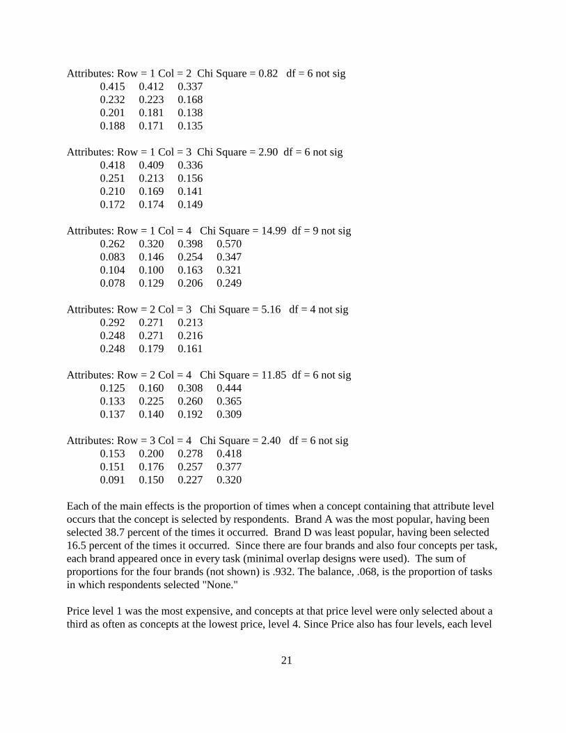
Each of the main effects is the proportion of times when a concept containing that attribute level

occurs that the concept is selected by respondents. Brand A was the most popular, having been

selected 38.7 percent of the times it occurred. Brand D was least popular, having been selected

16.5 percent of the times it occurred. Since there are four brands and also four concepts per task,

each brand appeared once in every task (minimal overlap designs were used). The sum of

proportions for the four brands (not shown) is .932. The balance, .068, is the proportion of tasks

in which respondents selected "None."

Price level 1 was the most expensive, and concepts at that price level were only selected about a

third as often as concepts at the lowest price, level 4. Since Price also has four levels, each level

22

appeared exactly once in each task, and the sum of the main effect proportions for Price is the

same as the sum for Brand.

The Size and Shape attributes only had three levels, so their levels sometimes appeared twice in

the same task. That produces proportions with smaller sums. If a level appears twice in the same

task, and if one of the concepts including it is selected, then the other concept is necessarily

rejected. When an attribute has fewer levels than the number of concepts per task, the sum of its

proportions is lowered. When making comparisons across attributes it is useful first to adjust

each set of proportions to remove this artifact. One way to do so is to divide all the proportions

for each attribute by their sum, giving them all unit sums.

All main effects are significant, yielding Chi Squares with probabilities less than .01. As with

other conjoint methods, it is often useful to summarize choice data with numbers representing the

relative importance of each attribute. With conjoint utility values we base importance measures

on differences between maximum and minimum utilities within each attribute. However, with

proportions, corresponding measures are based on ratios within attributes. To summarize the

relative importance of each attribute we might first compute the ratio of the maximum to the

minimum proportion for each attribute, and then percentage the logs of those ratios to sum to

100. Such summaries of attribute importance are only valid if respondents generally agreed on

the order of preference for the underlying levels. If respondents disagree about which levels are

preferred (which can often occur for attributes such as brand), such summaries of importance

from aggregate counts (or aggregate logit) can artificially bias estimates of attribute importance.

A more accurate analysis of attribute importances can result from utility values generated by

Latent Class or HB analysis.

The joint effects tables provide the same kind of information as main effects, but for pairs of

attributes rather than attributes considered one at a time. The joint effects tables also include

information about main effects. For example, consider the table for Brand and Price:

Price 1 Price 2 Price 3 Price 4 Avg

Brand A 0.262 0.320 0.398 0.570 0.387

Brand B 0.083 0.146 0.254 0.347 0.207

Brand C 0.104 0.100 0.163 0.321 0.172

Brand D 0.078 0.129 0.206 0.249 0.165

Average 0.132 0.174 0.255 0.372

We have labeled the rows and columns for clarity, and also added a row and column containing

averages for each brand and price. Comparing those averages to the main effects for Brand and

Price, we see that they are identical to within .001. The similarity between main effects and

averages of joint effects depends on having a balanced design with equal numbers of

23

observations in all cells. That will only be true with reasonably large sample sizes and when

there are no prohibitions.

None of the Chi Square values for the joint effects is statistically significant. The Chi Square

values indicate whether the joint effects contribute information beyond that of the main effects.

Thus we would conclude that, at least for this modest sample of approximately 100 respondents,

there is no evidence that the brands respond differently to differences in price. Another way of

saying the same thing is that within the table, all rows tend to be proportional to one another, as

are the columns.

Logit Analysis

CBC lets you select main effects and interactions to be included in each logit analysis. When

only main effects are estimated, a value is produced for each attribute level that can be

interpreted as an "average utility" value for the respondents analyzed. When interactions are

included, effects are also estimated for combinations of levels obtained by cross-classifying pairs

of attributes.

Logit analysis is an iterative procedure to find the maximum likelihood solution for fitting a

multinomial logit model to the data. For each iteration the log-likelihood is reported, together

with a value of "RLH." RLH is short for "root likelihood" and is an intuitive measure of how well

the solution fits the data. The best possible value is 1.0, and the worst possible is the reciprocal

of the number of choices available in the average task. For these data, where each task presented

four concepts plus a "None" option, the minimum possible value of RLH is .2.

Here is the output for a LOGIT computation, using the same data as above:

Iter 1 log-likelihood = -1471.20588 rlh = 0.24828






Converged.

Log-likelihood for this model = -1462.73822

Log-likelihood for null model = -1699.56644

Difference = 236.82822

Chi Square = 473.656

24

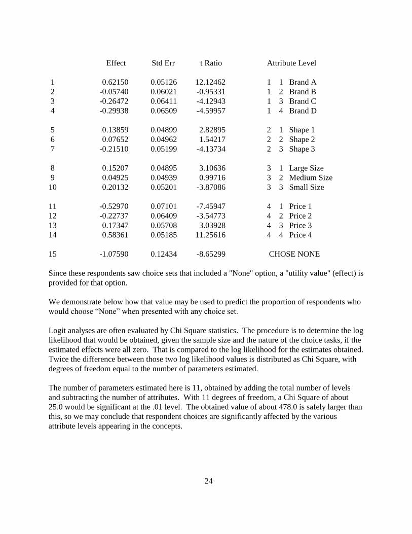
Effect Std Err t Ratio Attribute Level

1 0.62150 0.05126 12.12462 1 1 Brand A

2 -0.05740 0.06021 -0.95331 1 2 Brand B

3 -0.26472 0.06411 -4.12943 1 3 Brand C

4 -0.29938 0.06509 -4.59957 1 4 Brand D

5 0.13859 0.04899 2.82895 2 1 Shape 1

6 0.07652 0.04962 1.54217 2 2 Shape 2

7 -0.21510 0.05199 -4.13734 2 3 Shape 3

8 0.15207 0.04895 3.10636 3 1 Large Size

9 0.04925 0.04939 0.99716 3 2 Medium Size

10 0.20132 0.05201 -3.87086 3 3 Small Size

11 -0.52970 0.07101 -7.45947 4 1 Price 1

12 -0.22737 0.06409 -3.54773 4 2 Price 2

13 0.17347 0.05708 3.03928 4 3 Price 3

14 0.58361 0.05185 11.25616 4 4 Price 4

15 -1.07590 0.12434 -8.65299 CHOSE NONE

Since these respondents saw choice sets that included a "None" option, a "utility value" (effect) is

provided for that option.

We demonstrate below how that value may be used to predict the proportion of respondents who

would choose “None” when presented with any choice set.

Logit analyses are often evaluated by Chi Square statistics. The procedure is to determine the log

likelihood that would be obtained, given the sample size and the nature of the choice tasks, if the

estimated effects were all zero. That is compared to the log likelihood for the estimates obtained.

Twice the difference between those two log likelihood values is distributed as Chi Square, with

degrees of freedom equal to the number of parameters estimated.

The number of parameters estimated here is 11, obtained by adding the total number of levels

and subtracting the number of attributes. With 11 degrees of freedom, a Chi Square of about

25.0 would be significant at the .01 level. The obtained value of about 478.0 is safely larger than

this, so we may conclude that respondent choices are significantly affected by the various

attribute levels appearing in the concepts.

25

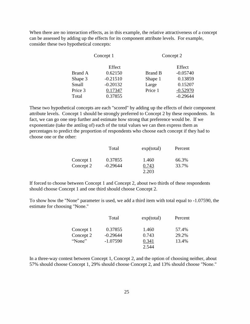
When there are no interaction effects, as in this example, the relative attractiveness of a concept

can be assessed by adding up the effects for its component attribute levels. For example,

consider these two hypothetical concepts:

Concept 1 Concept 2

Effect Effect

Brand A 0.62150 Brand B -0.05740

Shape 3 -0.21510 Shape 1 0.13859

Small -0.20132 Large 0.15207

Price 3 0.17347 Price 1 -0.52970

Total 0.37855 -0.29644

These two hypothetical concepts are each "scored" by adding up the effects of their component

attribute levels. Concept 1 should be strongly preferred to Concept 2 by these respondents. In

fact, we can go one step further and estimate how strong that preference would be. If we

exponentiate (take the antilog of) each of the total values we can then express them as

percentages to predict the proportion of respondents who choose each concept if they had to

choose one or the other:

Total exp(total) Percent

Concept 1 0.37855 1.460 66.3%

Concept 2 -0.29644 0.743 33.7%

2.203

If forced to choose between Concept 1 and Concept 2, about two thirds of these respondents

should choose Concept 1 and one third should choose Concept 2.

To show how the "None" parameter is used, we add a third item with total equal to -1.07590, the

estimate for choosing "None."

Total exp(total) Percent

Concept 1 0.37855 1.460 57.4%

Concept 2 -0.29644 0.743 29.2%

“None” -1.07590 0.341 13.4%

2.544

In a three-way contest between Concept 1, Concept 2, and the option of choosing neither, about

57% should choose Concept 1, 29% should choose Concept 2, and 13% should choose "None."

26

To see how LOGIT's output and COUNT's output are similar, we use the same procedure to

estimate the distribution of choices for four concepts differing only in brand, plus a "None"

option. The resulting numbers should be similar to the main effects for Brand as determined by

the COUNT module.

Effect exp(effect) Prop- From Diff-

ortion COUNT erence

Brand A 0.62150 1.862 0.400 0.387 0.013

Brand B -0.05740 0.944 0.203 0.207 -0.004

Brand C -0.26472 0.767 0.165 0.173 -0.008

Brand D -0.29938 0.741 0.159 0.165 -0.006

None -1.07590 0.341 0.073 0.068 0.005

Total 4.655 1.000 1.000 0.000

Although the estimates derived from logit analysis are not exactly the same as those observed by

counting choices, they are very similar. The differences are due to slight imbalance in the

randomized design, and the estimates produced by logit analysis are slightly more accurate. With

a larger sample size we would expect differences between the two kinds of analysis to be even

smaller.

CBC also comes with Sawtooth Software’s market simulator that automatically performs

calculations like those just described. The user provides specifications for products assumed to

be competing in the market. The Simulator adds up appropriate values for each product,

exponentiates their sums, and then percentages the results to provide estimates of shares of

choice. The Simulator computation includes two-way effects if they have been specified in the

corresponding LOGIT computation (two-way effects are not specified in the simple examples

above). The user may specify competitive sets of as many as 100 competitive products.

Again, we should emphasize that the aggregate logit routine included in the base CBC system is

an effective tool for summarizing the results of a CBC study. However, for developing

additional insights based on market segments and for developing more accurate market

simulators that deal better with such issues as the IIA property described earlier, we strongly

recommend Latent Class or HB estimation.

Evidence of Validity and Usefulness

Choice-based conjoint analysis has been in use for some time now, and evidence is mounting as

to its validity and usefulness.

Earlier in this paper we described our own first use of the method, in a series of studies for

Heublein, Inc., nearly three decades ago. Sometime later, we spoke with David Eickholt, the

27

marketing research manager responsible for those studies, who at that time was VP Marketing at

Heublein. With the benefit of a decade of hindsight, he reported that the results from those

studies were accurate in predicting the switching among brands and prices resulting from the

anticipated tax increase. He said that a critical aspect of those studies was their ability to deal

with interactions, revealing different demand curves for different brands and package sizes as

prices changed.

Another commercial experience with choice-based conjoint analysis was a study done for the

Chevron Chemical Company, and described in a paper presented to the American Marketing

Association's 1991 Advanced Research Techniques conference (Johnson and Olberts, 1991).

That study was also concerned with price, and considered multiple brands in each of several

different product categories. It revealed that even within a category, different brands can respond

very differently to price changes. Although we haven’t seen follow-up information regarding

ability to predict actual market responses to price changes, an author of the paper, Kathleen

Olberts of Chevron, reported that the results confirmed existing knowledge about the product

categories studied.

During 1991 and 1992, while developing CBC, we had the opportunity to participate with users

of pre-release versions of the software in several large-scale commercial studies. Those studies

dealt with a wide variety of products including household detergents, magnetic media, computer

peripherals, and cable TV services. In each case the client found CBC's results to be readily

interpretable and easy to use, and in each case the research firm conducting the study expressed

satisfaction with the technique.

More evidence has emerged suggesting that CBC can be an effective approach for predicting

actual buyer behavior. We recommend two papers from the 1999 Sawtooth Software

Conference, “Forecasting Scanner Data by Choice-Based Conjoint Models” (Feurstein and

Natter), and “Predicting Actual Sales with CBC: How Capturing Heterogeneity Improves

Results” (Orme and Heft). Furthermore, papers from Greg Rogers of Procter & Gamble are also

useful: “Validation and Calibration of Choice-Based Conjoint for Pricing Research” presented at

the 2003 conference and “The Importance of Shelf Presentation in Choice-Based Conjoint

Studies” presented at the 2004 conference.

28

References

Feurstein, Markus and Martin Natter (1999), “Forecasting Scanner Data by Choice-Based

Conjoint Models,” Sawtooth Software Conference Proceedings.

Green, Paul E. and V. Srinivasan (1990), "Conjoint Analysis in Marketing Research: New

Developments and Directions," Journal of Marketing 54, 4, 3-19.

Huber, Joel, D. R. Wittink, R. M. Johnson, and R. Miller (1992), "Learning Effects in Preference

Tasks: Choice-Based Versus Standard Conjoint," Sawtooth Software Conference Proceedings,

275-282.

Johnson, Richard M. and K. A. Olberts (1991), "Using Conjoint Analysis in Pricing Studies: Is

One Price Variable Enough?," American Marketing Association Advanced Research Technique

Forum Conference Proceedings, 164-173.

Louviere, Jordan J., and G. G. Woodworth (1983), "Design and Analysis of Simulated Consumer

Choice or Allocation Experiments: An Approach Based on Aggregate Data," Journal of

Marketing Research 20, 350-367.

Oliphant, Karen, T. C. Eagle, J. J. Louviere, and D. Anderson (1992), "Cross-Task Comparison

of Ratings-Based and Choice-Based Conjoint," Sawtooth Software Conference Proceedings,

383-394.

Orme, Bryan K (1998), “The Benefits of Accounting for Respondent Heterogeneity in Choice

Modeling,” technical paper available at www.sawtoothsoftware.com/techpap.shtml.

Orme, Bryan K. and Mike Heft (1999), “Predicting Actual Sales with CBC: How Capturing

Heterogeneity Improves Results,” Sawtooth Software Conference Proceedings.

the cbc system for choice-based conjoint · pdf filethe cbc system for choice-based conjoint...

Documents