the case of medical malpractice lawyers
TRANSCRIPT

Estimating the Degree of Expert�s Agency Problem:
The Case of Medical Malpractice Lawyers
Yasutora Watanabe�
Northwestern University
March 2007
Abstract
I empirically study the expert�s agency problem in the context of lawyers and their
clients. Incentives of lawyers and clients are misaligned in dispute resolution under
contingency fee arrangement with which lawyers receive a fraction of recovered payment
as compensation while bearing the legal cost. Lawyers prefer to pursue a case less
than their clients prefer as they incur all the legal costs and receive smaller fraction
of payment. In this paper, I measure the degree to which lawyers work in the interest
of their clients. To do so, I construct a bargaining model of dispute resolution that
nests two special cases as well as their convex combinations in which lawyers work in
their clients�best interests and in which they work in their own interests, and estimate
the model using data of medical malpractice disputes. The timing of dropped cases
identi�es the nesting parameter because cases are dropped more frequently and at earlier
timings if lawyers work in their own interests. I �nd that lawyers work almost perfectly
in their own interest. Then, I compute the cost of agency problem resulting from
misaligned incentives by simulating the �rst-best outcome using the estimated model.
Finally, I evaluate the impact of tort reform on contingency fee, and show that limitation
of contingency fee lower the joint surplus further.
�Department of Management and Strategy, Kellogg School of Management, Northwestern University,2001 Sheridan Road, Evanston, IL 60208. Email: [email protected]
1

1 Introduction
Expert agents can mislead their clients in their own interests due to lack of expertise on
the side of their clients. Experts such as lawyers, physicians, auto repairers, and real
estate agents are better informed of the services they provide than their clients. Due to
this asymmetry of information, clients make decision based on advices of experts or even
delegate their decision to the experts, and clients may not know or �nd it very costly to
verify if the experts worked in their best interests. As a result, experts have incentive to
work in their own interests instead of their clients�interests.
On the other hand, factors such as reputational concern, professional liability, capacity
constraint, and/or professional ethics mitigates the experts�agency problem to some extent.
The degree to which experts work in the interest of their clients depends on relative strength
of these factors and is an open empirical question. Existing studies either con�rms the
existence of the experts�agency problem or countering e¤ects of the mitigating factor, but
have not measured the relative strength.
In this paper I estimate the degree to which experts work in their client�s interest.
Speci�cally, I consider the experts�agency problem for the case of lawyers and their clients
in resolution of medical malpractice disputes. A plainti¤ in medical malpractice dispute
signs contingency fee contract with a lawyer. The incentives of the lawyer and the client are
misaligned in dispute resolution under contingency fee arrangement with which the lawyer
receives a fraction of recovered payment as compensation while bearing all the costs of legal
services. Since the client incur no cost of the lawyer�s services, the lawyer prefer to settle
the case earlier than the client prefers, and the lawyer has stronger incentive to drop a
case.1 Using data on timing of settlements and dropping, I answer the primary question of
this paper: What is the degree to which a lawyer work in the interest of a client?
Contingency fee is also an important policy issue in tort reform discussion, especially on
medical malpractice. Regulation on contingency fees are adopted by 15 states as of 20052
and are currently under consideration at the federal level.3 In spite of its policy importance,
little is known empirically about how regulation on contingency fee a¤ects the outcomes of
medical malpractice disputes such as legal costs, settlement payments, and probability of
1 In this paper, "drop" means that the side of the plainti¤ stops pursuing the case, which includes voluntarydismissal, settlement with zero payment without �ling of a lawsuit, and settlement with zero payment after�ling of a lawsuit. .
2See the database of state tort law reforms constructed by Avraham (2006). These regulations typicallyimpose a limit on the fraction lawyers can receive as contingency fee such as 40% and 33%.
3The House of Representatives passed the Help E¢ cient, Accessible, Low-Cost, Timely Healthcare(HEALTH) Act of 2003 in the 108th Congress, while the Senate voted against it. The bill has been reintro-duced in 2004 and 2005 and is currently pending. The Medical Care Access Protection Act of 2006 stalledin the Senate also includes regulation on contingency fee for plainti¤�s attorneys on medical malpracticecases.
2

lawsuits, as well as how it a¤ects the agency problem of lawyers and their clients. This is
another question I ask in this paper.
In order to answer these questions, I construct a bargaining model of dispute resolution
that nests two special cases as well as their convex combinations; one in which lawyers work
in the best interests of their clients, and one in which lawyers work for their own interests.
I estimate the model using a unique micro-level data on medical malpractice disputes.
The nesting parameter measures the degree to which incentives are misalignement. Using
the estimated model, I simulate the �rst-best outcome and measure the cost of agency
problem resulting from the misaligned incentive. Finally, I conduct a counterfactual policy
experiment of limiting contingency fees and assess the impact of the policy on outcomes
and welfare.
A plainti¤ (i.e. a patient) in a medical malpractice dispute retain a lawyer and adopt
contingency fee arrangement for vast majority of cases.4 A claim by the side of plainti¤
against a healthcare provider initiates a medical malpractice dispute. The plainti¤�s lawyer5
and the defendant engage in negotiations over the terms of settlement in the shadow of court
judgment. If the side of plainti¤ �les a lawsuit and the parties do not reach an agreement
or the side of the plainti¤ do not drop the case, they will face a judgment by the court,
which determines whether the defendant is liable and, if so, the award to the plainti¤. The
side of the plainti¤ can drop a case at any time during the process.
To study this process, I construct a dynamic bargaining model in which the plainti¤�s
lawyer and the defendant bargain over a settlement following Yildiz (2003, 2004) andWatan-
abe (2006). At any time during the negotiation, as long as the case has neither been settled
nor dropped, the plainti¤�s lawyer has the option of �ling a lawsuit that would initiate the
litigation phase. If the case is neither settle nor dropped during the litigation phase, the
case is resolved in court, where a jury verdict determines whether the defendant is liable
and, if so the award to the side of the plainti¤. In any period prior to the termination of
a dispute, the plainti¤�s lawyer and the defendant must pay the legal costs which I allow
to di¤er across the sides of the plainti¤ and the defendant and depending on whether or
not a lawsuit is �led. In particular, the legal costs are typically higher during the litigation
phase, which entails additional legal procedures with respect to the pre-litigation phase. I
do not consider expert�s agency problem for the side of the defendant because medical lia-
bility insurance companies who are well-informed of the legal issues and procedures makes
desicions for the defendant.4For example, Sloan et al (1993) reports that plainti¤s retained lawyers in 99.4 percent of the cases and
that contingency fee arrangement was adopted in 99.4 percent of the cases in Florida.5 I assume throughout the paper that the plainti¤�s lawyer is the decision maker for the side of the plainti¤.
This is a common assumption in the literature that is supported by surveys for individual clients (see, e.g.Sloan et al (1993) and Kritzer (1998)).
3
A parameter � 2 [0; 1] in the model re�ects the degree to which the lawyer work in theclient�s interest. Depending on the value of this parameter the model nests two special cases
and their convex combination; one in which the plainti¤�s lawyer work in the best interest
of the plainti¤ (� = 0), and one in which the lawyer work in her own interest (� = 1). In
the former case, the objective of the plainti¤�s lawyer is to maxmize the payment from the
defendant ignoring any legal cost incurred by the side of the plainti¤. In the latter case, the
objective of the plainti¤�s lawyer is to maximize a contingency fee fraction of payment from
the defendant minus the sum of per-period legal cost incurred by the side of the plainti¤.
I characterize the unique subgame-perfect equilibrium of this dynamic bargaining game.
Equilibrium outcomes specify (i) the lawyer�s decision of whether to �le a lawsuit and (ii)
if so the time to �ling, (iii) whether or not the case is dropped by the plainti¤�s lawyer,
(iv) whether or not the case is settled out of court, (v) the time to resolution by dropping
or by settlement, (v) the legal costs incurred, and (vi) the terms of settlement. Delaying
agreement is costly because of the per-period legal costs. However, the possibility of learning
new information makes delay valuable for both players. This fundamental trade-o¤ plays
an important role in the equilibrium characterization and is a key determinant of the time
to �ling and the time to settlement. Furthermore, I �nd that the more misaligned the
incentives of the plainti¤ and his or her lawyer are, the shorter the time to settlement as
well as to dropping and the higher the probability of dropping a case. This is because the
plaini¤�s lawyer takes her per-period cost more fully if their incentives are misaligned. This
property identi�es the nesting parameter in estimation.
I estimate the model using a unique data set on individual medical malpractice disputes.
The data set contains detailed information on the time, mode, cost, and terms of settlement
as well as the time of �ling lawsuit (if a lawsuit is �led) and the time of dropping (if a case
is dropped) for all medical malpractice disputes in Florida over the period 1985-1999. The
estimate for the nesting paramater � is 0.8128, which implies that the lawyers do not work
very much in the best interest of their clients.
I use the estimated structural model to compute the cost of agency problem resulting
from the incentive misalignment. To do so, I simulate the �rst-best outcome which cor-
responds to the case that the plainti¤�s lawyer maximize the payment from the defendant
minus the legal cost incurred.6 I �nd that the joint surplus for the side of the plainti¤ is
15% less compared to the �rt-best outcome. Under the �rst-best outcome, more cases are
litigated and the time to resolution increases. The legal costs of the both side increases, but
6Socially optimal outcome cannot be achieved in the model we estimate. In case the plainti¤�s lawyerwork in his/her interest, the lawyer only considers a fraction of the payment from defendant minus the legalcost. In this case, the lawyer is giving too much weight for the legal cost. In case the plainti¤�s lawyerwork in the plainti¤�s best interest, the lawyer ignores the legal cost she incurs. In this case, the legal costis underweighted.
4

the increase in payment to the side of the plainti¤ from the side of the defendant is larger
than the increase in cost.
Finally, I conduct couterfactural policy experiments and evaluate how regulation on
contingency fee arrangement a¤ects the outcomes of dispute resolution as well as the cost of
the agency problem. Speci�cally, I consider a limit on contingency fee at 20%. I �nd that
more cases are dropped, frequency of �ling of lawsuits decrease, and mean time to resolution
decreases. This is because the plainti¤�s lawyer receive less fraction of the payment as
compensation with such limit on fees while the per-period legal cost remains the same.
The expected join-surplus decreases by about 13% re�ecting a large decrease in expected
payment.
1.1 Literature
A small but growing empirical literature studies agency problem in expert services.7 Levitt
and Syverson (2006) compares home sales in which real estate agents are the owner of
the house and in which they are not, and found that houses are sold at higher price and
stayed longer on market in the former case. Gruber and Owings (1996) analyzed physicians�
likelihood of performing cesarean section delivery, and show a strong correlation between
decline in fertility and increase in cesarean, which they interpret as physician�s inducing
demand for cesarean by exploiting agency relationship. Iizuka (2006) investigates Japanese
prescrition market in which physician can sell drugs as well as prescribing it and �nd that
their prescriptions are in�uenced by the markup of the drugs. All these papers presents
evidence that agency problem exists in expert services. Hubbard (1998) studies auto repair-
eres�s emission inspection decision, and shows that auto repairers help to pass by expecting
customers to return rather than maximizing short run pro�ts by selling repairs. This paper
shows an evidence of factors that mitigates agency problem. None of the paper, however,
directly estimates the degree of incentive misalignment and quantify the cost of the agency
problem.
The paper also adds to the literature on empirical study of pre-trial bargaining.8 Using
data on the mode of resolution of civil disputes, Waldfogel (1995) estimates two-period
bargaining model with heterogenous belief. Sieg (2000) estimates barganing model with
asymmetric information to study the mode, cost, and terms of settlement in medical mal-
practice dispute using the same data set I use in this paper. Watanabe (2006) further
7Theoretical models of expert sercises includes Dranove (1988), Wolinsky (1993), Emons (1997), andFong (2005).
8See the surveys by Kessler and Rubinfeld (2005) and Spier (2007). Theoretical literature on agencyproblem regarding contingency fee contract includes Miller (1987), Rubinfeld and Scotchmer (1990), Danaand Spier (1993), Watts (1994), Hay (1996, 1997), Rickman (1999), Choi (2003), and Polinsky and Rubinfeld(2003). These papers employs two-period models which abstracts from learning during procedure. Hence,dropping during pre-trial bargaining is not considered.
5

investigate the dispute resolution process by constructing and estimating a multi-period
dynamic barganing model to study the timing of settlement and litigation in addition to
the mode, cost and terms of settlement. All of these papers, however, abstract from the
dropping decision and potential agency problem bewteen plainti¤ and plainti¤�s lawyer, and
do not utilize the data of dropped cases. Danzon and Lillard (1983) uses data of dropping
in medical malpractice disputes and �nd that limits on contingency fees lowers likelihood of
dropping signi�cantly. Helland and Tabarrok (2003) also uses data on medical malpractice
disputes and �nd that limit on contingency fees both lowers likelihood of dropping and
increases time to settlement. These two papers, however, are not interested in agency
problem and timing of dropping, which I address in this paper.
The remainder of the paper is organized as follows. In Section 2, I present the model
and characterize the equilibrium. Section 3 describes the data and Section 4 presents the
econometric speci�cation. Section 5 will contains the results of the empirical analysis.
2 Model
I consider a sequential bargaining model of legal dispute resolution with perfect-information
and stochastic learning. The players of the bargaining game are a plainti¤�s lawyer (p) and
a defendant (d).9 The plainti¤�s lawyer and the defendant bargain over the compensation
payment x 2 R+ from the defendant to the plainti¤ to resolve the dispute. Each player
i 2 fd; pg has linear von-Neumann-Morgenstern preferences over monetary transfer andlegal costs. Both players know the amount of the potential jury award V 2 R+, but theoutcome of the judgement is uncertain, i.e. the players do not know who will win the case
in the event of a trial.10 Hence, defendant pays V to the side of the plainti¤ if the plainti¤
wins the judgmen, while the defendant does not pay any amount otherwise. I denote the
plainti¤�s probability of prevailing by �.
Plainti¤s and his/her lawyers adopt contingency fee arrangement for vast majority of
9Throughout the paper, I assume the decision maker for the side of the plainti¤ as plainti¤�s lawyer.Sloan et al. (1993) �nds that plainti¤s "almost always followed their lawyer�s advice regarding settlement(p85)." They report that plainti¤s setted 100% of the cases when lawyer�s advice favored accepting and4.8% when lawyer�s advice favored rejecting. Another reason for this assumption is due to the informationalasymmetry between plainti¤s and his/her lawyers. Lawyers are experienced experts of the medical liabilitysystem, and the plainti¤s are less likely have better information than the lawyers. However, for the side ofthe defendant, I do not assume defendants�lawyers as decision makers because the defendants are primarilyinsurance companies and are well-informed and have expertise on dispute resolution.10 In the literature the uncertainty of the judgment is caused either (i) by the uncertainty of the winning
party (see e.g., Pries and Klein(1984)) or (ii) by the uncertainty of the award amount (see e.g. Spier (1992)).Implications of the model do not di¤er between (i) and (ii) because the expected award is what matters.I take the former assumption because I can better explain the data in which a large proportion of casesconcludes with no jury award at the court judgment.
6

the medical malpractice cases in Florida11, while defendants�legal councils charge an hourly
legal fee. The contingency fee arrangement entitles the plainti¤�s lawyers to a fraction of
the money received from the defendant only if a positive payment is received. I denote the
fraction by ; hence a plainti¤�s lawyer receives fraction of the defendant�s payment to
the side of the plainti¤ as compensation for the legal services they provide, and the palinti¤
receives the remaining fraction 1� .
Timing and Phases The bargaining game has two multi-period phases depending on
whether the plainti¤�s lawyer has �led a lawsuit or not: the pre-litigation phase (Phase O)
and the litigation phase (Phase L). The game starts with Phase O at period t = 0: Players
bargain every period until they reach an agreement. Phase O has a �nite number of periods
T <1, due to the statute of limitation at period t = T +1 <1, after which the plainti¤�sclaim to recover is barred by law. The plainti¤ has an option of �ling a lawsuit in Phase O
as long as no agreement has been reached and the case has not been dropped. The �ling
of a lawsuit moves the game to Phase L. Thus, in Phase O, a case may be either �led
(leading to Phase L), dropped (without �ling a lawsuit), settled (without �ling a lawsuit),
or terminated by the statute of limitations.
The plainti¤�s endogenous decision to �le a lawsuit initiates Phase L. Let tL 2 f0; :::; Tgdenote the date of the �ling of lawsuit. Once the plainti¤�les a lawsuit, the case is processed
in court towards the judgment scheduled T + 1 periods after the date of �ling, that is date
t = tL+T +1 <1 . While the case is processed in court, it can always be dropped by the
plainti¤ or settled by both parties until t = tL+T: Failure to reach a settlement agreement
by t = tL + T results in the resolution by the court judgment at t = tL + T + 1.
Information and Beliefs The model is a game of perfect information. As described
above, the players can observe all the actions of the other player. The information revealed
is also commonly observed by both players. Hence, there is no asymmetric information. The
players, however, do not have a common prior over the probability that the plainti¤ will
win the case (�). This asymmetry in initial beliefs may be due for example to di¤erences in
each party�s perception of the relative ability of his or her lawyer or to di¤erences in opinion
about the predisposition of potential juries.
I assume that the players�beliefs of the probability of the plainti¤�s prevailing � 2 [0; 1]follow beta distributions, a �exible as well as tractable distribution with support [0; 1] that
is widely used in statistical learning models on Bernoulli trial process. Player i�s initial
belief, denoted by bi0; are represented by Beta(�i; � � �i); where 0 < �d < �p < �:12 A
11Sloan et al. (1993) reports that 99.4% of the cases adpoted contingency fee arrangement in their Surveyof Medical Malpractice Claimants conducted in Florida during 1989-1990.12See Yildiz (2003, 2004) for a similar learning mechanism. Arrival of information is deterministic in his
7

prelitigation phase (length T )
litigation phase (length T )
statute of limitation (T+1 )
judgment (tL+T+1 )filing lawsuit (tL )
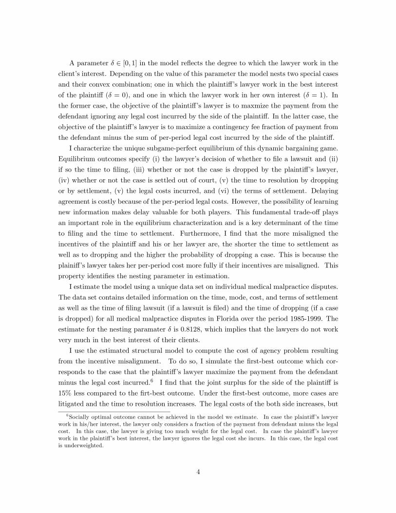
Figure 1: Diagram of Model Structure. The plainti¤ and the defendant start bargainingover a settlement in pre-litigation stage. At any time in pre-litigatioin stage, as long as theplainti¤ has not dropped the case or no agreement has been reached, the plainti¤ has theoption of �ling a lawsuit that endogenously determine tL and would initiate the litigationstage. If neither a lawsuit is �led, the case is dropped, nor a settlement is reached by Tin pre-litigation phase, the case is no longer valid due to statute of limitation. If neitheragreement is reached nor the case is dropped during the litigation stage, the case is resolvedby court judgment at tL + T + 1:
common parameter � represents the �rmness of belief as explained later. Thus, at the
initial date, the players have expected probability of plainti¤�s prevailing as
E(bp0) =�p�for the plainti¤, and
E(bd0) =�d�for the defendant.
At the beginning of each period t in Phase J 2 fO;Lg, information related to winningprobability (such as the result of a third party medical examination or testimony by an
expert witness) arrives with probability �J . I denote an arrival of information at t by
nt 2 f0; 1g, where nt = 1 means arrival of information while nt = 0 represents no arrival.
model, while it is stochastic in my model.
8

The cumulated amount of information at period t is denoted by nt 2 f0; :::; tg, and therefore
nt = nt�1 + nt:
Information is either in favor of or against the plainti¤. I denote the content of the
arrived information nt by mt 2 f0; 1g: The content is for the plainti¤ if mt = 1;while
mt = 0 means the arrived information is against the plainti¤, and
mt =
(0
1
with probability 1� �with probability �;
where � is not known to the players. The cumulated information in favor of the plainti¤
is denoted by mt 2 f0; :::; ntg, leading to
mt = mt�1 + ntmt
where mt is multiplied by nt since the content of information matters only if information
arrives.
Players update their beliefs according to Bayesian updating as follows: The beliefs at
period t, denoted by bpt and bdt , follow Beta(�p +mt; � � �p + nt �mt) and Beta(�d +mt;
�� �d + nt �mt) respectively. Hence, at period t; the expectations on the probability � of
plainti¤�s prevailing on the judgement are
E(bpt ) =�p +mt
�+ nt
and
E(bdt ) =�d +mt
�+ nt:
The players use these expectations as their estimates of �. The �rmer the beliefs (i.e., the
higher the �rmness of belief parameter �), the less is the impact of the information obtained
in the legal process. By modelling beliefs this way, I can capture the relative impact of new
learning on prior beliefs. The information environment I have described above is common
knowledge to both players. For notational convenience, I let kt = (nt;mt) 2 f0; tg � f0; tgdenote the information state.
Stage Games In Phase O, players play the following stage game in every period t 2f0; :::; Tg. At the beginning of each period, information arrives with probability �Ot and
does not arrive with probability 1��Ot. The information is such that it a¤ects the outcomeof the judgment (e.g., the result of third-party medical examination) and is commonly
9

observed by both players. Then, the plainti¤�s lawyer chooses whether to drop the case or
continue it. If she chooses to drop the case, the case is resolved with no payments being
made from defendant to the side of the plainti¤. Otherwise, nature chooses the proposer,
with probability � for the plainti¤ and 1�� for the defendant. The chosen party proposesthe amount of compensation payment x, which will be either accepted or rejected by the
other party. If accepted, the game concludes with the proposed amount of money x being
transferred from the defendant to the side of the plainti¤, and the dispute is resolved. In
such a case, the plainti¤�s lawyer receives x and the plainti¤ receives (1 � )x. If the
proposal is rejected, the plainti¤ chooses whether or not to �le a lawsuit. The case moves to
Phase L if the plainti¤ �les a lawsuit, while it remains in Phase O and the same stage game
is repeated if the plainti¤ chooses not to �le. If the case is neither �led nor settled during
the T periods, the statute of limitation renders the claim by the plainti¤ to be ine¤ective.
After the side of the plainti¤ �les a lawsuit, the parties play the following stage game
in every period t 2 ftL; :::; tL + Tg until the court judges on the case at t = tL + T + 1.
At the beginning of each period, information that a¤ects the outcome of the judgment
arrives with probability �Lt and does not arrive with probability 1 � �Lt. Then, the
plainti¤�s lawyer chooses whether to drop the case or continue it. If she chooses to drop
the case, the case is resolved with no payments being made from defendant to the side of the
plainti¤. Otherwise, nature again chooses the proposer, with probability � for the plainti¤
and 1 � � for the defendant. The chosen party proposes the amount of compensation
payment x, which will be either accepted or rejected by the other party. If accepted, the
game terminates with the proposed amount of money being transferred from the defendant
to the side of the plainti¤, and the dispute is resolved. In such a case, , the plainti¤�s
lawyer receives x and the plainti¤ receives (1� )x. If rejected, the case remains in PhaseL and the same stage game is repeated until t = tL + T:
I allow the rates of information arrival to di¤er across phases. One of the reasons for
di¤ering rates stems from the �discovery process.�In this process, both parties can employ
a variety of legal devices to acquire information on the case that follows the �ling of a
lawsuit.
I denote per-period legal costs at period t in Phases O and L for player � 2 fd; pgby CiOt 2 R+ and CiLt 2 R+ respectively. I assume that these legal costs are drawn
independently in each period t from identical distributions. I allow the distribution of
per-period costs to di¤er depending on whether or not the plainti¤ has �led a lawsuit.
In particular, the legal costs of both sides are typically higher in the litigation phase,
which entails additional legal procedures with respect to the pre-litigation phase. The
distributions from which per-period costs are drawn in Phases O and L are denoted by
GCO(�) and GCL(�). The realizations of the per-period costs only a¤ect the total legal costs,
10
and they do not a¤ect the equilibrium stopping timing and settlement terms because players
make desicions based on expeted legal cost of the subsquent periods.
I consider a common time-discount factor denoted by � 2 [0; 1].
A Parameter to Measure the Degree of Incentive Misalignment As discussed
above, plainti¤s�lawyers use a contingency fee arrangement, while defendants�legal councils
charge an hourly legal fee. The contingency fee arrangement entitles the plainti¤�s lawyers
to a fraction 2 [0; 0:5)13 of the money received from the defendant only if a positive
payment is received. Because of this deferment, the plainti¤ incurs no additional legal
cost by delaying agreement because the plainti¤�s lawyer incurs the legal cost. Hence,
the plainti¤ and his/her lawyer�s incentive are not aligned. The plainti¤ prefer to pursue
a case much longer than her lawyer prefer. The plainti¤s�s objective is to maximize the
expected payment from the defendant, while the lawyer always considers the cost as well
as the payment.
The main objective of this paper is to measure the degree to which lawyers and their
clients� incentives are misaligned, and I will measure this with the following parameter
� 2 [0; 1]: If a lawyer behaves perfectly in the interst of her plainti¤, she maximizes theexpected payment and does not consider per-period legal cost. If payment is x, such lawyer�s
payo¤ can be written as
u0 = (1� )x:
If a laywer behaves in her best interest, she considers the legal cost and only fraction of
the payment. Hence, we can write it as
u1 = x� Cpj :
where j 2 fO;Lg. My interest is to measure what the true payo¤ system is for the plainti¤�slawyer, and these two cases are the special cases in which the lawyer are perfectly working
in the interest of her client and in which she work in her own interest. Since these two
cases are the extreme ones, I can consider a convex combination of these two cases with a
parameter �, which can be written as
u� = � � u1 + (1� �) � u0 (1)
= (1� � � + 2� )x� �Cpj
Now, � = 1 implies that a lawyer behaves in her interest and � = 0 implies that a lawyer
behaves in the plainti¤�s interest. Hence, � mesures the degree to which the incentive of
13 I impose this assumption because contingency fee are below 50% for vast majority of cases.
11

the lawyers and the plainti¤ are misaligned. For notational convenience, I de�ne function
A(�) as
A(�) � 1� � � + 2� :
2.1 Equilibrium Characterization
The model is a dynamic game with perfect information. Thus, I employ subgame-perfect
equilibrium as the equilibrium concept. Because the model has a �nite number of peri-
ods, backward induction provides us with a characterization of the unique subgame-perfect
equilibrium. I start the analysis from the last stage in Phase L, and move to Phase O.
2.1.1 Phase L (Litigation Phase)
In order to characterize the unique subgame perfect equilibrium by backward induction,
I start my analysis from the date of the judgment by the court at the end of Phase L.
Recall that a Phase L subgame is reached only if the case is litigated at some period during
Phase O. Let tL 2 f0; :::; Tg denote the date of �ling the lawsuit which is an endogenouslydetermined. If the players cannot settle by date tL + T , the judgement by the court at
t = tL + T + 1 determines the outcome of the last stage. Since two decisions are made in
each period in Phase L, we de�ne two continuation values for each player. Let V it�tL(kt)
denote the continuation value for player i 2 fp; dg at the beginning of date t in Phase Lwith information state kt, and V
it�tL(kt) the continuatoin value after dropping decision by
plainti¤�s lawyer and before settlement decision at the end of the period t. Note that the
subscript is t� tL, which is the number of periods in Phase L so that V i1 (ktL) corresponds
to the continuation value at the �rst period in Phase L that will be on the right hand side
of the Bellman equation in Phase O. The continuation value of the judgment is
V pT+1(ktL+T+1) = A(�)E[bpT+tL ]V
V dT+1(ktL+T+1) = �E[bdT+tL ]V
where A(�)V is the amount plainti¤�s laywer obtains if she win the case and V is the
amount paid the defendant to the side of the plainti¤. The plainti¤ will have the di¤erence
(1�A(�))V: The term E[bpT+tL ] is the expected probability of winning based on the belief
of the plainti¤�s lawyer with her information set at one period before judgement.
Having above V iT+1(ktL+T+1) as �nal values, I can obtain Vit�tL(kt) and V
it�tL(kt) by
applying backward induction. The equilibrium in Phase L subgame is characterized in the
Proposition 1 below.
Proposition 1 In the unique subgame perfect equilibrium given kt and tL,
12
1. the payo¤ of the players at t 2 ftL + 1; :::; tL + Tg in Phase L are expressed as
V pt�tL(kt) = max�0; V
pt�tL(kt)
V dt�tL(kt) =
(0
Vdt�tL(kt)
if 0 > Vpt�tL(kt)
otherwise.
where
Vpt�tL(kt) = ��max
n�A(�)Edt
hV dt+1�tL(kt+1)� C
dL
i; Ept
�V pt+1�tL(kt+1)� �C
pL
�o+(1� �)�Ept
�V pt+1�tL(kt+1)� �C
pL
�;
Vdt�tL(kt) = ��Edt
hV dt+1�tL(kt+1)� C
dL
i+(1� �)�max
�� 1
A(�)Ept�V pt+1�tL(kt+1)� �C
pL
�; Edt
hV dt+1�tL(kt+1)� �C
pL
i�:
2. the plainti¤ �s lawyer drops the case at t 2 ftL + 1; :::; tL + Tg in Phase L i¤
0 > Vpt�tL(kt)
3. the players settle at t 2 ftL + 1; :::; tL + Tg in Phase L i¤
0 � Ept [Vpt+1�tL(kt+1)� �C
pL] +A(�)E
dt [V
dt+1�tL(kt+1)� C
dL]:
4. given that players settle at t 2 ftL + 1; :::; tL + Tg in Phase L, the payment is
xt =
(��Edt
�V dt+1�tL(ktS+1)� C
dL
�� 1A(�)E
pt
�V pt+1�tL(ktS+1)� �C
pL
� if the plainti¤ is a proposer
if the defendant is a proposer,
Proof. See Appendix A
This proposition characterizes the subgame perfect equilibrium in Phase L: The ex-
pression for V pt�tL(kt) in 1 is the continuation value at the beginning of the period when
plainti¤�s lawyer faces the dropping decsion. As described in 2, plainti¤�s lawyer drops a
case if her interim continuation value Vpt�tL(kt) is below 0. In such a situation, both sides
have 0 as their continuation value. Interim continuation value after dropping decision and
before settelment decision Vit�tL(kt) is obtained by solving for random-proposer barganing.
Note that expectations are indexed by player because two players have di¤erent beliefs over
the probability of winning at judgment.
The identify of the proposer do not a¤ect the settlement decision as can be seen in 3.
The amount of payment depends on the identify of the proposer as in 4. This arises because
13
the players choose to settle if the joint surplus of settlement today is larger than the joint
surplus of continuing the case. The compensation payment depends on the identity of the
proposer because the recognized proposer obtains all of the surplus. This is true even in the
extreme case that plainti¤�s lawyer work in the interest of her client (i.e. A(�) = 1� ) anddo not take per-period legal costs into consideration. Delaying agreement is still costly for
her because she misses the bene�ts of the saving of the defendant�s legal costs that indirectly
increases compensation payment. Therefore, delaying agreement is costly for both players,
and quick settlement is preferable. However, the possibility of learning new information
makes delay valuable, since this information enhances the probability of a settlement, which
in turn generates positive surplus for both players. This fundamental trade-o¤ plays an
important role in the equilibrium characterization and is a key determinant of the timing
of settlement.
Dropping decision is simply an individual rationality constraint for the plainti¤�s lawyer
at each period. If there is no learning, the continuation values for the plainti¤�s lawyer
increases monotonically over time as can be seen from 1. This monotonicity implies that if
the value is negative at period t, the value is also negative for any period t0 < t, i.e. if a
case is to be dropped at t, it must be dropped at any earlier date t0. Hence, all dropping
occurs only in the initial period if there is no learning. Therefore, dropping in periods other
than the initial period only occurs with learning at arrival of new information against the
plainti¤�s side. In such case, continuation value stays positive for �rst several periods, and
it become negative at the arrival of unfavorable information.
The proposition also shows that dropping and settlement decisions are directly a¤ected
by the degree of incentive misalignment �. Increase in � decreases the continuation value of
the plainti¤�s lawyer in two ways; through increase in per-period cost and through decrease
in A(�). Decrease of A(�) lowers Vpt�tL(kt) because the expected award at judgement
Ept [A(�)V ] decreases corrspoding to change in A(�). Thus, the larger � is, the smaller
Vpt�tL(kt) is, and the more likely tha the case is dropped. In other words, plainti¤�s lawyer
prefer to drop a case at earlier date if her incentives is less aligned. In the extreme case
that the lawyer works perfectly in her client�s interest (� = 0), the case is never dropped.
Similar intuition works for the e¤ect of incentive alignment and settlement decision. The
expression in 3 can be rewritten as
Et[�CpL + C
dL] � Ept [V
pt+1�tL(kt+1)] +A(�)E
dt [V
dt+1�tL(kt+1)];
where the left-hand side is expected per-period legal cost which is not indexed by player
because players have common belief over the distribution of cost. The right-hand side is
the expected surplus from continuation. Increase in � increase the value of the left-hand
14

side, and decreases the value of the right hand side14. Hence, the less aligned the incentives
are (the larger � is), the shorter it takes to reach a settlement on average. The plainti¤�s
lawyer who considers her own legal cost more seriously and focusing more on payments to
herself, which is much smaller than the payment to the plainti¤, prefer to settle at earlier
dates.
2.1.2 Phase O (Pre-Litigation Phase)
Let W it (kt) denote the continuation value for player i 2 fp; dg at the beginning of date t in
Phase O with information state kt. Again, I start from the last stage of Phase O subgame.
The maximum number of periods in Phase O is T ; after which the claim by the plainti¤
loses its value due to the statute of limitation. Hence, each player has continuation payo¤
of 0 at date T + 1, i.e.,
W p
T+1(kT+1) =W d
T+1(kT+1) = 0:
I compute W it (kt) by applying backward induction and having the above as �nal values.
In Phase O, the plainti¤ has an option of litigating a case at any date t 2 f0; :::; Tg.Solving the value function in Proposition 2 up to the �rst period in Phase L, I can obtain
the continuation value of the Phase L subgame, V i1 (kt). Note that this continuation value
of litigation does not depend on the date of litigation tL itself but does depend on the
information state kt at period t.
First, I will look at the �ling decision by the plainti¤�s lawyer because �ling decision is
the last decsion to be made in a period. The plainti¤�s lawyer chooses to litigate at the end
of date t if and only if
Et�V p1 (kt+1)� �C
pL
�� Et
�W pt+1(kt+1)� �C
pO
�;
where the left-hand side is the payo¤ from �ling a lawsuit and the right-hand side is the
payo¤ from stay in pre-litigation phase. Hence, the continuation value for the plainti¤ at
the end of date t is written as
Y pt (kt) = �max�Et�V p1 (kt+1)� �C
pL
�; Et
�W pt+1(kt+1)� �C
pO
�;
where Y pt (kt) denotes an interim continuation value for the plainti¤�s lawyer after the set-
tlment decision and before the �ling decision in period t in Phase O given state kt. The
defendant�s continuation value depends on the �ling decision of the plainti¤�s lawyer de-
14Though A(�) increase in �, A(�)Edt [V
dt+1�tL(kt+1)] decrease in � because E
dt [V
dt+1�tL(kt+1)] is always
negative and decreases in �:
15

scribed above, and is written as
Y dt (kt) =
(�Et
�V d1 (kt+1)� CdL
��Et
�W dt+1(kt+1)� �C
pO
� if Et�V p1 (kt+1)� �C
pL
�� Ept
�W pt+1(kt+1)� �C
pO
�otherwise,
where Y dt (kt) denotes an interim continuation value for the plainti¤�s lawyer after the settl-
ment decision and before the �ling decision in period t in Phase O given information state
kt. I can then conduct the exact same analysis for settlement and dropping decision as
I did for Phase L; and the subgame-perfect equilibrium for Phase O is characterized in
Proposition 2.
Proposition 2 In any subgame perfect equilibrium given kt;
1. the payo¤s of the players at t 2 f0; :::; Tg in Phase O are expressed as
W pt (kt) = max
�0;W
pt (kt)
W dt (kt) =
(0
Wdt (kt)
if 0 > Wpt (kt)
otherwise.
where
Wpt (kt) = �max
n�A(�)Y dt (kt); Y
pt (kt)
o+ (1� �)Y pt (kt);
Wdt (kt) = �Y dt (kt) + (1� �)max
�� 1
A(�)Y pt (kt); Y
dt (kt)
�:
2. the players settle at t 2 f0; :::; Tg in Phase O i¤
Y pt (kt) +A(�)Ydt (kt) � 0:
3. the plainti¤ litigates at t 2 f0; :::; Tg in Phase O i¤
Et [Vp1 (ktL+1)] � Et
�W pt+1(kt+1)
�:
4. given that players settle at t 2 f0; :::; Tg in Phase O, the payment is
xt =
(�Y dt (kt)Y pt (kt)
if the plainti¤ is a proposer
if the defendant is a proposer,
Proof. See Appendix B
16
This proposition characterizes the subgame perfect equilibrium in Phase O: The mechan-
ics of the settlement and dropping decisions are exactly the same as for the characterization
for Phase L. The only di¤erence is that the cost of delay and the possibility of learning in
the next period depend on the plainti¤�s decision to �le or not at the end of each period.
The decision to �le a lawsuit by the plainti¤ is also derived from a trade-o¤ between the
cost of delay and the possibility of learning. The cost of delaying �ling has two components.
One is the per-period legal cost of the pre-litigation phase, because the total length of the
underlying game becomes one period longer if �ling is delayed by one period. Even though
the plainti¤ incurs no legal cost per period, this delay still impacts him because minimizing
the defendant�s legal cost may result in a higher compensation payment to the plainti¤. The
second component is the cost of delay due to discounting. The plainti¤ prefers to obtain
the continuation value of the Phase L subgame earlier, since a one-period delay in �ling
costs him (1� �)V p1 (�) when no information arrives. The bene�t of delaying �ling by oneperiod is that the parties have one more period to obtain new information and hence reach
an agreement. Thus, the plainti¤ prefers to stay in Phase O longer if CiO are small and �
is large, while low �Ot provides an incentive for the plainti¤ to �le early.
3 Data
The Florida Department of Financial Services, an insurance regulator of the Florida state
government, collects a detailed micro-level data set on medical malpractice disputes in
Florida. A statute on professional liability claims requires medical malpractice insurers to
�le a report to the Department on all of their closed claims once the claim is resolved. The
report contains detailed information on the dispute resolution process, as well as individual
case characteristics. The information on the dispute resolution process includes important
dates (calender date of occurrence, initial claim, �ling of lawsuit, resolution either by drop-
ping, settlement, or by court judgement), settlement payments (or award by the court in
case of resolution by court judgment), and total legal costs incurred by the defendants.
The information on case characteristics includes patient characteristics (e.g. age and sex),
defendant characteristics (e.g. defendant type, specialty, and insurance policy), and the
characteristics of injury (e.g. severity and place of occurrence). Hence, this data set con-
tains detailed information on all the variables of interest, i.e., if and when a lawsuit is �led,
whether or not the case is settled out of court or dropped, the time to resolution, the legal
costs incurred and the terms of settlement.
My sample of observations consists of 5,379 claims against physicians15 which were
15Claims against hospitals, HMOs, dentists, ambulance surgical centers, and crisis stabilization units areexcluded from my sample to control for the heterogeneity of the plainti¤.
17

Number ofObservations
ResolutionProbability
MeanCompensation
Mean DefenseLegal Cost
Dropped withoutLawsuit
783 0.1460(0)
7; 330(23; 023)
Dropped afterLawsuit
751 0.1400(0)
40; 370(44; 978)
Settledwithout Lawsuit
472 0.088314; 266(303; 917)
9; 047(15; 014)
Settledafter Lawsuit
2,887 0.537303; 402(379; 909)
53; 989(88; 887)
Resolved by Judgmentwith Positive Award
127 0.024541; 832(620; 722)
127; 966(113; 147)
Resolved by Judgmentwith No Award
359 0.0670(0)
83; 182(87; 268)
Total 5,379 1.000203; 210(343; 922)
45; 047(77; 794)
Compensation payments and legal costs are measured in 2000 dollars. Numbers in parenthesesprovides standard deviations.
Table 1: Descriptive Statistics I - Resolution Probability, Payments and Legal Costs
resolved between October 1985 and July 1999.16 Following Sieg (2000), I restrict attention
to cases with the defendant�s legal cost exceeding $1,000 and which were not dropped during
the litigation process.17 Because the timing and disposition of cases di¤er greatly depending
on the severity of the injury, I restrict attention to the cases in which injuries resulted in
permanent major damage to or death of the patient.
Tables 1 and 2 show the descriptive statistics of all the variables I use for estimation. In
my data, 28.6% of the cases are dropped or settled with zero payment, 62.5% of the cases
were settled by parties, and the remaining 9.1% of the cases were resolved by judgement by
the court. Regarding dropped and settled cases, only one senveth of settled cases settled
without �ling a lawsuit and majority of settled cases are settled after �ling a lawsuit, while
the proportion of cases dropped without �ling a lawsuit and after �ling a lawsuit are about
the same around 14%. For the judged cases, the defendants were three times more likely
to win the judgment (i.e., award was zero). Mean compensation payments were similar for
the cases that were settled after �ling a lawsuit and those that were settled without �ling
16During this period, there were no major changes in state law pretaining to resolution of medical mal-practice disputes.17This procedure eliminates small cases.
18

Time toFiling
Time to Resolutionafter Filing
Total Time toResolution
Droppedwithout Filing
� � 4:81(3:22)
Droppedafter Filing
2:30(2:31)
7:36(4:51)
9:66(5:09)
Settledwithout Filing
� � 3:23(2:41)
Settledafter Filing
2:48(2:26)
7:45(4:55)
9:93(5:16)
Resolved by Judgmentwith Positive Award
2:69(2:67)
11:41(6:61)
14:10(7:17)
Resolved by Judgmentwith No Award
2:50(3:21)
9:69(5:17)
12:19(6:24)
Total2:45(2:38)
7:75(4:76)
8:81(5:57)
Numbers are in quarters of a year. The numbers in parentheses provide standard deviations.
Table 2: Descriptive Statistics II - Timings
a lawsuit (around $300,000).
Legal costs for defendants substantially di¤ered across modes of resolution. Defense
lawyers usually charge based on the amount of time they spent. It is not surprising to
�nd that the mean of the defense legal costs correlates strongly with the mean time to
resolution as displayed in Table 2. Mean of defence legal costs for cases settled without a
lawsuit is about one-�fth of the cases settled after a lawsuit. This di¤erence correlates with
the shorter mean time to resolution as in Table 2. The cases settled after �ling a lawsuit have
a signi�cantly higher mean cost ($53,989) compared to the settled cases without a lawsuit
($9,047). Similary, the cases dropped after �ling a lawsuit have a signi�cantly higher mean
cost ($40,370) compared to the cases dropped without a lawsuit ($7,330). Among the cases
resolved by court judgement, mean defense costs are more than 50% higher for the cases
won by the plainti¤s than the cases won by the defendants, which again corresponds to the
longer time to resolution.
Mean time to �ling a lawsuit, which corresponds to the periods spent in the pre-litigation
phase, is similar across the dropped cases, the settled cases, and the cases resolved by court
judgment. The time to resolution di¤er between the cases settled after �ling and the cases
19

0
0.05
0.1
0.15
0.2
0.25
0.3
0.35
1 2 3 4 5 6 7 8 9 10 11 12
quarters
fract
ion
Time to dropping without a lawsuit
Time to settlement without a lawsuit
Time to filing a lawsuit
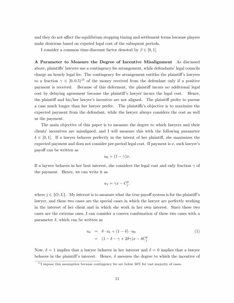
Figure 2: Histogram of Time to Dropping, Settlement and Filing. Fractions of time todropping without a lawsuit, settlement without a lawsuit, and �ling a lawsuit add up toone. This isbecause cases are either 1) dropped without a lawsuit, 2) settled without alawsuit, or 3) resolved after a lawsuit is �led.
resolved by the judgment. This di¤erence results from the di¤erence in time to resolution
after �ling lawsuit. The cases settled without a lawsuit, which correspond to settlement in
pre-litigation phase, spend longer periods in the pre-litigation phase than the �led cases on
average, and the cases dropped without a lawsuit spends even longer time on average about
4.81 quarters.
Figure 2 provides the histogram of �ling, dropping, and settlement in pre-litigation
phase. Note that the sum of the fractions for �ling, dropping, and settlement add up
to one because each case is either �led, dropped without a lawsuit, or settled without a
lawsuit. In Florida, the statute of limitation regarding a medical malpractice cases is two
years. Hence, more than 95% of the cases are �led or settled without �ling a lawsuit before
the ninth quarter.18
A fraction of cases �ling lawsuits in pre-litigation phase and a fraction of cases settling
without lawsuits have a common pattern. In both the hazard rate increases signi�cantly
18The remaining cases may be due, for example, to invervening medical complications that entail anautomatic extension of the statute of limitations.
20

0
0.02
0.04
0.06
0.08
0.1
1 2 3 4 5 6 7 8 9 10 11 12 13 14 15 16 17 18 19 20 21 22 23 24
quarters
fract
ion
Time to dropping after filing
Time to settlement after filing
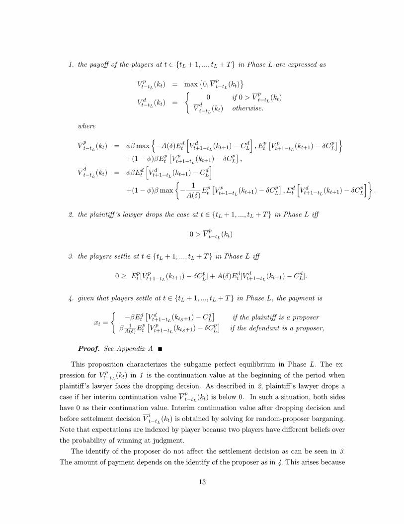
Figure 3: Histogram of Time to Dropping and Settlement after Filing. Fraction of droppedand settled Cases will add up to one. Time is counted from the date of �ling a lawsuit inquarters. Cases exceeding 6 years are counted in the bin of the 24th quarter.
at the second quarter and gradually increases over time. Corresponding to a high hazard
rate after the second quarter, the histogram re�ects that more than 30% of cases are �led
in the second quarter before the fraction declines rapidly over time. Regarding the time to
settlement without a lawsuit, the decline after the second quarter is much slower as a result
of the lower hazard rate. Compared to the �led and settled cases, hazard rate for dropping
is lower and dropped cases spends longer time in pre-litigaiton phase.
Figures 3 presents more details on the time to settlement and dropping after �ling
lawsuits. The hazard rates for settlement and dropping are almost the same and they
increase over time until 9th quarter as can be seen from the very similar patterns in the
�ture. Ninety percent of settled cases are settled in 13 quarters, and less than 5% of cases
are settled after 16 quarters. Similary, ninety percent of dropped cases are dropped in 13
quarters, and less than 5% of cases are settled after 17 quarters.
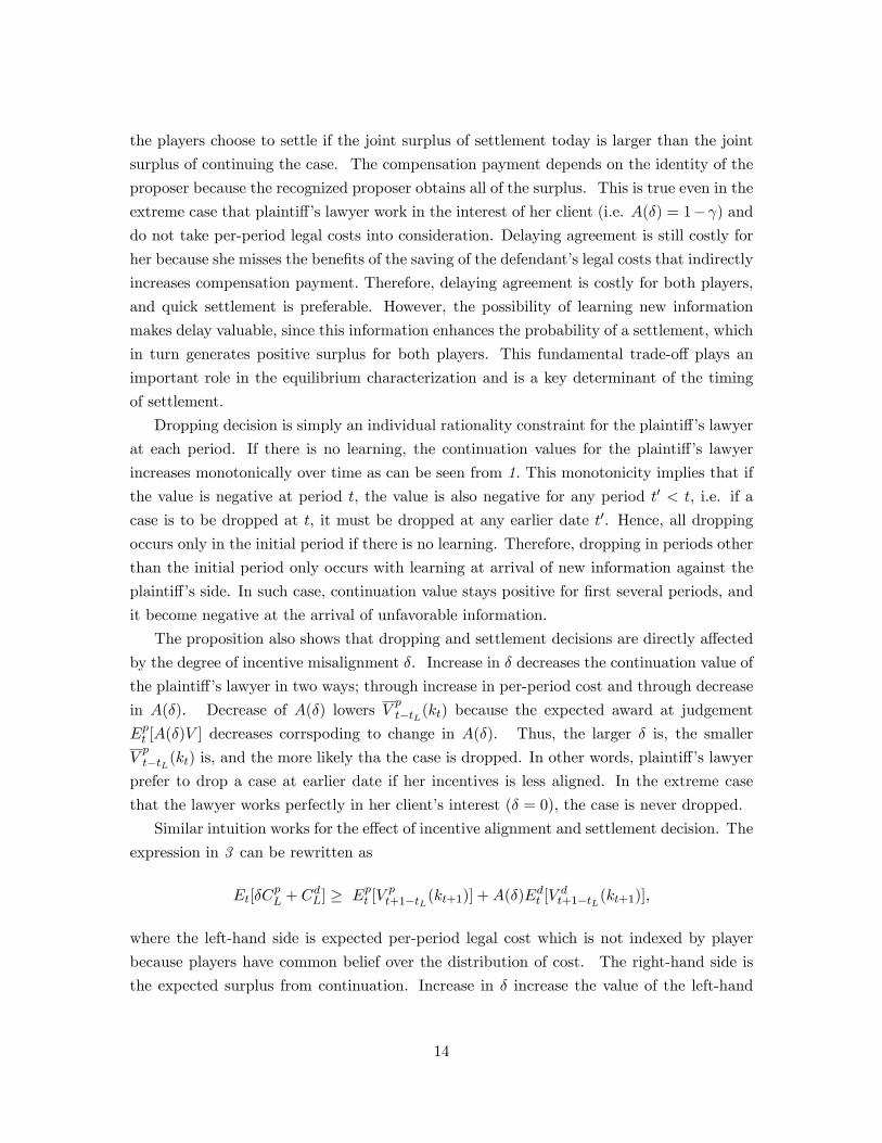
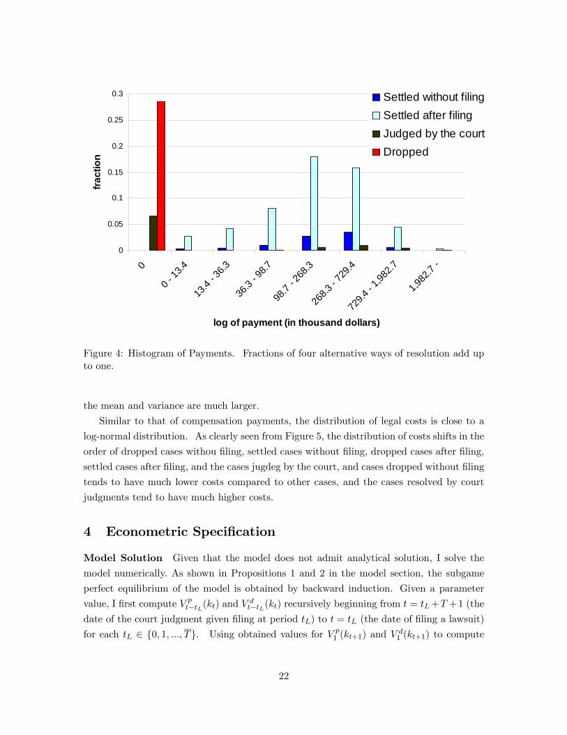
Compensation payments have very high variance. Figure 4 presents the histogram
of (log) compensation payments from the defendant to the plainti¤. Of the total cases,
about 6.7% of them concluded with judgment in favor of the defendant and 28.6% of them
are dropped, thus, have zero payments. The amount of positive payments have very
high variance, and the shape of the distribution is close to log-normal distribution. The
distributions of settled cases without �ling and of settled cases after �ling are similar. More
than 40% of the cases are with payments between $98,700 and $729,400. The distribution
for the cases judged with positive award is also similar to the log-normal distribution, while
21
0
0.05
0.1
0.15
0.2
0.25
0.3
0
0 13
.4
13.4
36.3
36.3
98.7
98.7
268
.3
268.3
729
.4
729.4
1,98
2.7
1,982
.7
log of payment (in thousand dollars)
fract
ion
Settled without filingSettled after filingJudged by the courtDropped
Figure 4: Histogram of Payments. Fractions of four alternative ways of resolution add upto one.
the mean and variance are much larger.
Similar to that of compensation payments, the distribution of legal costs is close to a
log-normal distribution. As clearly seen from Figure 5, the distribution of costs shifts in the
order of dropped cases withou �ling, settled cases without �ling, dropped cases after �ling,
settled cases after �ling, and the cases jugdeg by the court, and cases dropped without �ling
tends to have much lower costs compared to other cases, and the cases resolved by court
judgments tend to have much higher costs.
4 Econometric Speci�cation
Model Solution Given that the model does not admit analytical solution, I solve the
model numerically. As shown in Propositions 1 and 2 in the model section, the subgame
perfect equilibrium of the model is obtained by backward induction. Given a parameter
value, I �rst compute V pt�tL(kt) and Vdt�tL(kt) recursively beginning from t = tL+T +1 (the
date of the court judgment given �ling at period tL) to t = tL (the date of �ling a lawsuit)
for each tL 2 f0; 1; :::; Tg. Using obtained values for V p1 (kt+1) and Vd1 (kt+1) to compute
22

0
0.02
0.04
0.06
0.08
0.1
0.12
0.14
0 2.
9
2.9 4
.9
4.9 8
.1
8.1 1
3.4
13.4
22.0
22.0
36.3
36.3
59.9
59.9
98.7
98.7
162
.8
162.8
log of legal cost (in thousand dollars)
fract
ion
Dropped without filing
Settled without filing
Dropped after filing
Settled after filing
Judged by the court
Figure 5: Histogram of Defense Legal Costs. Fractions of �ve alternative ways of resolutionadd up to one.
continuation value in the case that plainti¤�s lawyer �les a lawsuit at the end of the period
t, I compute W pt (kt) and W
dt (kt) recursively from t = T to t = 0. Due to relatively small
size of the state space, continuation values at each state are computed exactly.
Unobserved Heterogeneity I allow for unobserved heterogeneity in several dimensions.
First, I consider unobserved heterogeneity in the time to judgment after �ling, T . Given
two cases that are resolved by court judgment, the time to judgment T can signi�cantly
di¤er across cases. For example, congestion in the legal system in a particular jurisdiction
a¤ects the time to judgement T . Hence, I need to assume an unobserved heterogeneity on
the exogenous parameter T . Because there is no reason to belive that settled cases would
have systematically di¤erent distribution of time to judgment compared with judged case, I
estimate the distribution of the time to judgment nonparapmetrically using the data of the
cases that are judged by the court. This estimation is outside of the model, and it is simply
a histogram of time to judgment. I denote the cumulative distribution function (CDF) of
T by FT (�):
23
The statute of limitation period T , which is also exogenous in the model, also di¤ers
across cases though the statute of limitation date for medical malpractice litigation in
Florida is set at 2 years. The legally determined statute of limitation period is not the
actual length of time player can bargain without �ling a lawsuit. The statute of limitation
is legally counted from the date of the occurrence of incident, but the bargaining does not
necessarily begin on the date of occurrence. For example, a plainti¤ may begin bargaining
8 months after the occurrence of the incident, which leaves him 16 months before �ling if
the legal length of the statute of limitation is 24 months. I assume T to follow a negative
binomial distribution which is a �exible distribution with discrete support. I denote their
CDFs by FT (�) with parameters 0T and 1T :Another dimension of unobserved heterogeneity is on jury awards. Cases that are re-
solved by court judgment may have very di¤erent potential jury awards V depending on the
unobserved characteristics of the case, composition of the juries, and other factors. Hence,
I consider unobserved heterogeneity in V: I assume that V follows a log-normal distribution
FV (�) with mean and variance denoted by �V and �2V .I also consider unobserved heterogeneity in the distribution of per-period legal costs
GCO(�) and GCL(�):I assume these cost distributions as Gamma distributions with scaleparameters !O and !L, and common shape parameter ! for computational tractability, and
model unobserved heterogeneity as parameters !O and !L to follow parametric distributions
as following. These distributions di¤ers across cases due to factors such as the law �rm the
plainti¤ and defendant employ or some other unobserved characteristics. I assume the
mean of distributions GCO(�) (or expected per-period legal cost), !O! to follow log-normaldistributions whose cumulative distribution functions are denoted by FC(�) with parameters�C and �
2C . Thus, given a realization of mean of the distribution GCO(�), we only need to
estimate ! because a draw from FC determines one parameter. Given a case, the per-period
legal cost after �ling a lawsuit is most likely to increase due to the increase in the hours
worked by the lawyers to prepare more documentations. Hence, I reparametrize !L by a
new parameter � so that E[CiL] = (1 + �)E[CiO]; or !L ! = (1 + �)!O!: Since the degree
of the increase of the per-period legal cost depends on the characteristics of the case, as
well as the law �rm employed for the case, I assume � to have unobserved heterogeneity.
Therefore, I consider unobserved heterogeneity in �, and assume it to follow log-normal
distributions whose cumulative distribution function is denoted by F�(�) with parameters�� and �
2�. Similar to the argument for GCO(�), we only need to estimate ! due to a draw
from F� determining one parameter. For the side of the plainti¤ and the defendant, I draw
parameters of cost distributions independently from the above distribtuion FC(�) and F�(�)as discussed later as an identi�cation assumption. For notational convenience, I denote the
realization of unobserved heterogeneity by Z = fCO; �; V; T; Tg:
24

Estimation I use the equilibrium characterization derived by Propositions 1 and 2 to
compute the likelihood contribution of each observation. Because I can compute the con-
ditional probabilities of equilibrium decisions (as above), I can now construct the likelihood
function. The contribution to the likelihood function of each observation in the sample is
equal to the probability of observing the vector of endogenous events (x; tS ; tL; s; l) given
the vector of the parameters � = f�; �d; �p; �; �O0; �O1; �L0; �L1; �; �; FT ; FT ; FC ; F�; FV g.Because I consider unobserved heterogeneity in Z = fCO; �; �; V; T; Tg, I need to conduct aMonte Carlo integration over these variables Z in order to obtain the likelihood which can
be written as
L(�jx; tS ; s; tL:l) =Z Z Z Z Z
Pr(x; tS ; s; tL; ljZ; �)dFCdF�dFTdFTdFV ;
where Pr(x; tS ; s; tL; ljZ; �; i) is computed using the conditional probabilities computedabove as follows. (i) For the cases dropped without �ling a lawsuit, Pr(x; tS ; s; tL; ljZ; �)isI take the log of above probability and sum them over all the elements in the sample to
obtain the log-likelihood.
For parameters (contingency fee), I used = 0:33 following Sieg (2000). I used
� = 0:995 for time discount factor for a quarter.
Identi�cation I need an indenti�cation assumption for the legal cost of the plainti¤�s
lawyer because data of the plainti¤�s legal cost is not available. I assume that the parameters
for cost distribution for the side of the plainti¤ is drawn from the same distribution as the
defendant�s legal costs, i.e. Cpjt and Cdjt are iid draw from di¤erent cost distributions whose
parameters are iid draw from the same distribution FC and F�: This is a natural assumption
considering that market for legal service is comepetitive. These distributions are identi�ed
from the variation of data of the defendants�s total legal costs and time a case spent in
Phase O and Phase L:
Data of settlement payments conditional on �ling and settlement date (or awards if a
case is resolved by court judgment) along with legal cost identi�es the distribution of awards
FV . Parameter for relative bargaining power � is identi�ed from the settlement payment
conditional on �ling and settlement date because �ing and settlement timing determines
surplus whose allocation between a proposer and the other party is determined by �:
The distribution of time to judgement from �ling FT is non-parametrically identi�ed by
the data of the time to judgment of the cases judged by the court with a natural assumption
that time to jusgement are not systematically di¤erent among judged, settled, and dropped
cases. Similarly, the winning rate of the plainti¤ at court judgement identi�es �, which
is estimated outside of the model. The distribution of time to statute of limitation FT is
25

identi�ed by the data of time to �ling with the distributional assumption. Parameters for
information arrival rates and initial pirors are identi�ed from the variation of data of the
settlement timings in Phase O and Phase L, and fractions of cases judged by the court, and
farctions of cases settled in Phase O and in Phase L.
Finally, as I have discussed in the model section, the parameter of incentive misalignment
� a¤ects the fraction of cases dropped and the timing of dropping and settlement. The
more misaligned the incentives are (the higher � is), the shorter the time to settlement
and dropping are as well as the more cases to be dropped. Hence, � is identi�ed from the
fraction of cases dropped and the timing of dropping given the identi�caiton of the rest of
the parameter as discussed above.
5 Results
5.1 Parameter Estimates
Parameter estimates are presented in Table 3. The estimates of the weighting parameter
� 2 [0; 1] is 0.8128. This implies that the plainti¤�s lawyers works more in their short-runinterest than in the best interest of their clients. This result can be interpreted in several
ways because there are several factors that provides inceintive for a plainti¤�s lawyer not
to work only in their short-run interest such as reputational concern, professional liability,
capacity constraint, or altruism. The result shows that these factors do not work very
strongly in this context though I cannot distinguish between which of these factors are
contributing.
Di¤erence in beliefs is very large at the initial stage, but their beliefs are very weak.
Plainti¤�s belief on probability of his winning is �p=� = 0:9554, while mean of defendant�s
belief on probability of plainti¤�s winning is �d=� = 0:0315. These beliefs are very weak
because the �rmness parameter � is very small at 0:0021. For example, if an information
against the plainti¤ would arrive in period 1, i.e. nt = 1 and mt = 0, the plainti¤�s belief
would change from 0.9554 to 0:0001+00:0021+1 = 0:0001. This implies that the learning plays an
important role. Also, an assumption that only "one piece" of information can arrive in a
period might be the reason for this result.
Arrival rate of information at t in pre-litigation stage is �Ot = 0:0066 + 0:0073 � t,
and that of litigation stage at t0-th period from litigation is �Lt0 = 0:0064 + 0:0231 � t0:
Thus, information are more likely to arrive as procedure advances. Also, the arrival rate
is much higher once lawsuit is �led. This is very natural result because �ling of lawsuit
institutionally in�uences the arrival of new information a¤ecting the outcome of judgment.
Other parameter I allow to di¤er across stage is the per period legal cost. Mean of
defence legal cost per period in pre-litigation phase is $2,762 with estimated variance of
26

Parameter Estimates� 0.8128 (0.0377)�d 0.0001 (0.0001)�p 0.0021 (0.0001)�O0 0.0066 (0.1075)�O1 0.0073 (0.0101)�L0 0.0064 (0.0451)�L1 0.0231 (0.0023)� 0.2613 (0.1930)� 0.6053 (0.3549)� 0.0022 (0.0001)�C 6.7278 (0.4909)! 0.7966 (5.1032)�2C 0.4219 (0.1475)�� -0.9013 (0.2372)�2� 3.4108 (0.4460)�V 13.2785 (0.4797)�2V 0.9360 (0.2209)cf1 15.4099 (1.4625)cf2 3.7688 (2.8544)cf3 9.8190 (0.5432) 0T 7.5491 (0.3328) 1T 0.6488 (0.0012)Log-likelihood 40504.5961
Table 3: Maximum Likelihood Estimates
27

$4,252. On average, legal cost per period increases 2.115 times after �ling of lawsuit and
mean legal cost per period in litigation phase is $5,842. Mean of damage V 19 is $905,738,
which is much larger than the mean settlement and mean judgement in the data. I need to
work further so that these number will be closer to the one in the data. Finally, the relative
bargaining power between plainti¤ and defendant is caputred by �.20 The estimate of
� being 0.6053 implies that plainti¤ have relatively stronger bargaining power though the
standard error is relatively large.
5.2 Model Fit
As a result of estimation, I �nd that the model �ts all aspect of the data well. I provide
the �t of the model regarding the time to settlement and �ling, as well as the compensation
payments for di¤erent modes of resolution. In Figures 6 and 7, I present the �t of the model
to the data on the time to dropping and �ling. The model replicates the dynamic patterns
of �ling and dropping in pre-litigation very well as shown in Figure 6. In particular, the
model �ts the data on the time to �ling, which increase sharply in period 2 and decreases
gradually, very well. Regarding settlement in the pre-litigation phase, the magnitude of
the fraction is captured correctly. Though I do not report the �t of the settlement in pre-
litigaton phase in Figure 6, the degree of the �t is similar to those of the dropping and
�ling.
Figure 7 shows the �t of the model on the time to settlement and dropping after �ling
a lawsuit. The model captures the shape of the data, which increases for the �rst several
period and then declines gradually. The di¤erence between the predicted fractions of cases
settling and the data in the �rst three periods and the last several periods may result from
the linearity assumption on the rate of arrival. This assumption may have prevented the
model from capturing some factors in the data.
6 Comparison to the First-Best Outcome
In this section, I compare the estimated model with the �rst-best outcome for the side of
the plainti¤. I de�ne the �rst-best outcome as the outcome under which the expected joint
surplus for the side of the plainti¤ is maximized. The join surplus for the side of the plainti¤
is the expected payment from the side of the defendant to the side of the plainti¤ minus
the legal cost incurred by the plainti¤�s lawyer.
19This is the amount plainti¤ will (potentially) receive if he won the judgment at trial.20 In the model, � is a probability that the plainti¤ will be recognized as a proposer. This is a measure of
bargaining power in the model because proposer always bene�ts from proposer advantage, while the otherparty is only o¤ered the amout equal to his continuation payo¤.
28

0
0.05
0.1
0.15
0.2
0.25
0.3
0.35
1 2 3 4 5 6 7 8 9 10 11 12
quarters
fract
ion
Time to dropping without a lawsuit
Time to dropping (fit)
Time to filing a lawsuit
Time to filing (fit)
Figure 6: Histogram of Timing in Pre-Litigation Phase
0
0.02
0.04
0.06
0.08
0.1
1 2 3 4 5 6 7 8 9 10 11 12 13 14 15 16 17 18 19 20 21 22 23 24
quarters
fract
ion
Time to settlement after filing (data)
Time to settlement (fit)
Time to dropping after filing (data)
Time to dropping (fit)
Figure 7: Histogram of Timing after Filing
29

Fitted Model First BestFraction of Dropped Cases in Phase O 11.3% 7.4%Fraction of Filed Cases 77.5% 80.8%Mean Time to Resolution (quarters) 7.77 8.10Mean of Legal Cost (dollars) 29,885 31,557Mean Payment (dollars) 1,180,982 1,448,523Joint Surplus (dollars) 1,151,098 1,416,937
Table 4: First-best outcome
The outcome is computed by simulating the model setting parameter values to = 1
and � = 1. This corresponds to a situation in which a plainti¤�s lawyer can buy out a
case. Under these parameter values, the side of the plainti¤ is internalizing the full legal
cost that was incurred the plainti¤�s lawyer and 100% of the payment rather than fraction
under contingency fee arrangement.
Table 4 summarizes the comparison of �tted model with the simulated �rst-best out-
come. Under the �rst-best outcome, about 4% less fraction of cases are dropped before
�ling a lawsuit, and 3% more lawsuits are �led. The mean time to resolution increases
by 0.3 quarters. Re�ecting higher fraction of lawsuits, less dropped cases, and longer time
to resolution, the mean legal cost increases by 5.8%. However, the increase of the legal
cost is very small compared to the increase in payment of 22.7% from 1,180,982 dollars to
1,416,937 dollars. Hence, the expected joint-surplus under �rt-best outcome is 23.1% larger
at 1,416,937 dollars.
7 Policy Experiments
Finally, I conduct a counter-factual policy experiment to limit the contingency fee. Regu-
lation on contingency fees are adopted by 15 states as of 200521 and are currently under
consideration at the federal level.22 In spite of its policy importance, little is known empir-
ically about how regulation on contingency fee a¤ects the outcomes of medical malpractice
disputes such as legal costs, settlement payments, and probability of lawsuits, as well as
how it a¤ects the agency problem of lawyers and their clients.
For the couter-factual experiment, I set the limit of the contingency fee to 20% ( = 0:2),
and simulate the distribution of equilibrium outcome using the estimated parameters. With
21See the database of state tort law reforms constructed by Avraham (2006). These regulations typicallyimpose a limit on the fraction lawyers can receive as contingency fee such as 40% and 33%.22The House of Representatives passed the Help E¢ cient, Accessible, Low-Cost, Timely Healthcare
(HEALTH) Act of 2003 in the 108th Congress, while the Senate voted against it. The bill has been reintro-duced in 2004 and 2005 and is currently pending. The Medical Care Access Protection Act of 2006 stalledin the Senate also includes regulation on contingency fee for plainti¤�s attorneys on medical malpracticecases.
30

Fitted Model ExperimentFraction of Dropped Cases in Phase O 11.3% 12.7%Fraction of Filed Cases 77.5% 76.3%Mean Time to Resolution (quarters) 7.77 7.66Mean of Legal Cost (dollars) 29,885 29,020Mean Payment (dollars) 1,180,982 943,123Joint Surplus (dollars) 1,151,098 914,103
Table 5: Policy experiment on limit on contingency fee
the limit at 25%, the fraction of payment to plainti¤�s lawyer decreses from 33% to 25%,
while the per-period legal costs incurred by her remains the same. This implies that the
plainti¤�s lawyer have less incentive to maximize the join-surplus because she can receive
even smaller fraction of the payment.
Table 5 summarizes the comparison of the �tted model with the outcome of the counter-
factual experiment. The policy of limiting the contingency fee would increase the number
of case to be dropped in pre-litigation phase from 11.3% to 12.7% and reduces the �ling
of lawsuits from 77.5% to 76.3%. The mean time to resolution also decreaes from 7.77
quarters to 7.66 quarters. These changes are consisten with the change in the lawyer�s
incentive due to the limit of contingency fee. Re�ecting shorter time to resolution, more
frequent dropping, and less �ling of lawsuit, legal cost also decreases from 29,885 dollars to
29,020 dollars. However, the decrease in mean payment by 20.1% is much larger than the
saving of legal cost. This results in the decrease of join surplus by 20.6% from 1,151098 to
1,002997.
8 Appendix
Appendix A Proof of Proposition 1Consider two separate cases depending on whether the players will settle or continue.
First, consider the case of Ept [Vpt+1�tL(kt+1)� �CpL] + A(�)Edt [V
dt+1�tL(kt+1)� CdL] > 0;
in which players do not settle. I will show that they will not settle under this condition
using proof by contradiction. Suppose that the players settle in period t with monetary
transfer xt. The plainti¤ agrees only if A(�)xt � �Ept�V pt+1�tL(kt+1)� �C
pL
�, while the
defendant agrees only if �xt � �Edt�V dt+1�tL(kt+1)� C
dL
�. This requires 0 = ��1(xt �
xt) � 1A(�)E
pt
�V pt+1�tL(kt+1)� �C
pL
�+ Edt
�V dt+1�tL(kt+1)� C
dL
�. This contradicts with
Ept [Vpt+1�tL(kt+1)� �CpL] + A(�)Edt [V
dt+1�tL(kt+1)� CdL] > 0, which proves that the players
will not settle at t. Hence, the continuation value of each player before the nature chooses
31

proposr at date t denoted as Vit�tL(kt) can be written as
Vpt�tL(kt) = �Ept
�V pt+1�tL(kt+1)� �C
pL
�;
Vdt�tL(kt) = �Edt
hV dt+1�tL(kt+1)� C
dL
i:
Second, consider the case of Ept [Vpt+1�tL(kt+1) � �CpL] � �A(�)Edt [V dt+1�tL(kt+1) � CdL];
in which players settle. Both players accept an o¤er if it gives them at least their
continuation value. If the plainti¤ is recognized as a proposer, she chooses to o¤er
xt = �Edt�V dt+1�tL(kt+1)� C
dL
�; the defendant�s continuation value, which is the lowest
o¤er the defendant accepts. In such case, the plainti¤�s lawyer�s payo¤ is �A(�)xt, whichis larger than her continuation value, i.e., �A(�)xt = �A(�)�Edt
�V dt+1�tL(kt+1)� C
dL
��
�Ept [Vpt+1�tL(kt+1)� �C
pL]. In the case that the defendant is a proposer, he chooses to o¤er
xt =1
A(�)�Ept
�V pt+1�tL(kt+1)� �C
pL
�, which is the lowest o¤er the plainti¤�s lawyer accepts.
In such case, the defendant�s payo¤ is �xt, which is larger than his continuation value, i.e.� 1A(�)�E
pt
�V pt+1�tL(kt+1)� �C
pL
�� �Edt
�V dt+1�tL(kt+1)� C
dL
�. Thus, in equilibrium, the
proposer o¤ers the continuation value of the opponent, and the opponent accepts. The
continuation value of each players before the nature chooses proposer at date t will be
Vpt�tL(kt) = ��(�A(�)Edt
hV dt+1�tL(kt+1)� C
dL
i) + (1� �)�Ept
�V pt+1�tL(kt+1)� �C
pL
�;
Vdt�tL(kt) = ��Edt
hV dt+1�tL(kt+1)� C
dL
i+ (1� �) 1
A(�)�(�Ept
�V pt+1�tL(kt+1)� �C
pL
�):
Combining both cases, the continuation value is written as
Vpt�tL(kt) = ��max
nA(�)(�Edt
hV dt+1�tL(kt+1)� C
dL
i); Ept
�V pt+1�tL(kt+1)� �C
pL
�o+(1� �)�(Ept
�V pt+1�tL(kt+1)� �C
pL
�;
Vdt�tL(kt) = ��Edt
hV dt+1�tL(kt+1)� C
dL
i+(1� �)�max
�� 1
A(�)Ept�V pt+1�tL(kt+1)� �C
pL
�; Edt
hV dt+1�tL(kt+1)� C
dL
i�:
At the beginning of the period t, the plainti¤�s lawyer chooses whether to drop the case
or not. She drops the case if her continuation payo¤ is lower than 0 because she can
always have outside option of 0 by dropping the case Hence, the continuation values at the
beginning of period t are written as
V pt�tL(kt) = max�0; V
pt�tL(kt)
The continuation value for the defendant depends on the decision of the plainti¤�s lawyer.
32

If she drops the case, the defendant has no obligation to pay, while his continuation value
is Vdt�tL(kt) if plainti¤�s lawyer do not drop the case. Thus, the defendant�s continuation
value is written as
V dt�tL(kt) =
(0
Vdt�tL(kt)
if 0 > Vpt�tL(kt)
otherwise.:
�
Appendix B Proof of Proposition 2I consider two separate cases depending on whether the players will settle or continue
the case.
First, consider the case of Y pt (kt) > �A(�)Y dt (kt), in which players do not settle. Sup-pose that the players settle in period t with monetary transfer x. The plainti¤�s lawyer
agrees only if A(�)x � Y pt (kt), while the defendant agrees only if x � �Y dt (kt). This
requires 0 = x� x � 1A(�)Y
pt (kt) + Y
dt (kt). This contradicts with Y
pt (kt) > �Y dt (kt), which
proves that the players will not settle at t. Hence, the continuation value of each players
before settlement decision at date t will be
Wit(kt) = Y it (kt):
Now, consider the case of Y pt (kt) � �A(�)Y dt (kt); in which players settle. Each playeraccepts an o¤er if and only if it gives him/her at least his/her continuation value, and a
party recognized by nature to propose chooses to o¤er this continuation value because it
is least costly o¤er to be accepted by the other party. If the plainti¤�s side is recognized
as the proposer, she o¤ers Y dt (kt) to the defendant, which is defendant�s continuation value
and defendant accepts. In this case, the plainti¤�s lawyer receives �A(�)Y dt (kt): If thedefendant is recognized as the proposer, he o¤ers x = 1
A(�)Ypt (kt) with which the plainti¤�s
lawyer receives her continuation value of Y pt (kt). Thus, I can write the continuation value
of each player beforeat the settlement decision at date t as
Wpt (kt) = �
h�A(�)Y dt (kt)
i+ (1� �)Y pt (kt);
Wdt (kt) = �Y dt (kt) + (1� �)
�� 1
A(�)Y pt (kt)
�:
Combining the above two cases, I can rewrite the continuation value as
Wpt (kt) = �max
n�A(�)Y dt (kt); Y
pt (kt)
o+ (1� �)Y pt (kt);
Wdt (kt) = �Y dt (kt) + (1� �)max
�� 1
A(�)Y pt (kt); Y
dt (kt)
�:
33

At the beginning of the period t, the plainti¤�s lawyer chooses whether to drop the case or
not. Same as in Phase O; she drops the case if her continuation payo¤ is lower than 0 be-
cause she can always have outside option of 0 by dropping the case Hence, the continuation
value for the plainti¤�s lawyer at the beginning of period t is written as
W pt (kt) = max
�0;W
pt (kt)
The continuation value for the defendant depends on the decision of the plainti¤�s lawyer.
If she drops the case, the defendant has no obligation to pay, while his continuation value is
Wdt (kt) if plainti¤�s lawyer do not drop the case. Thus, the defendant�s continuation value
is written as
W dt (kt) =
(0
Wdt (kt)
if 0 > Wpt (kt)
otherwise.
�
Appendix C Computation of Conditional Choice ProbablitiesIn Chapter 2, I characterized the equilibrium outcome on the time, mode, cost, and
terms of settlement, as well as the time of �ling a lawsuit (if a lawsuit is �led). However,
the outcomes are contingent on the realization of the state of information kt = (nt;mt) 2f0; :::; tg�f0; :::; tg which is not observable to the econometrician. Thus, from the perspec-tive of the econometrician, the litigation timing tL, the resolution timing tS , the compen-
sation payment x, and the total legal cost are all random variables because they depend
on the (unobservable) realization of kt. Hence, I �rst compute the conditional probability
of observing the realization of such random variables in order to compute the likelihood
contribution of each observation.
Let dDOt (nt;mt), dSOt (nt;mt), dDLt (nt;mt; tL), dSLt (nt;mt; tL), and dFIt (nt;mt) denote
the indicator function respectively for dropping in Phase O, settlement in Phase O, dropping
in Phase L, settlement in Phase L, and �ling of a lawsuit at period t. Using the results of
Propositions 1 and 2, these indicator functions are written as
dDOt(nt;mt) = I�Wpt (nt;mt) < 0
;
dSOt(nt;mt) = InY pt (nt;mt) +A(�)Y
dt (nt;mt) < 0
o;
dFIt(nt;mt) = I�EtV
p1 (nt+1;mt+1) > EtW
pt+1(nt+1;mt+1)
;
dDLt(nt;mt; tL) = I�Vpt�tL(nt+1;mt+1) < 0
;
dSLt(nt;mt; tL) = InEtV
pt+1�tL(nt+1;mt+1) +A(�)EtV
dt+1�tL(nt+1;mt+1)� �CpL �A(�)C
dL < 0
o;
where dDOt (nt;mt) = 1, dSOt (nt;mt) = 1, dDLt(nt;mt; tL) = 1, dSLt (nt;mt; tL) = 1,
34

dFIt (nt;mt) = 1 indicate dropping in Phase O, settlement in Phase O, dropping in Phase
L, settlement in Phase L, and litigation at period t given (nt;mt) and (nt;mt; tL), while 0
indicate otherwise. In computing equilibrium, we assume the rates of information arrival
as �Ot = �O0 + �O1t and �Lt = �L0 + �L1t: Let qOt (nt;mt) denote the probability of being
in state kt = (nt;mt) 2 f0; :::; tg � f0; :::; tg in Phase O, and let qLt (nt;mt; tL) denote the
probability of being in state kt in Phase L given the litigation date of tL < t. I can compute
qOt recursively as follows:
qO0 (0; 0) = 1;
qOt (n;m) = �Ot�qOt�1(n� 1;m� 1)
��1� dSOt (n� 1;m� 1)� dDOt (n� 1;m� 1)
� �1� dFIt (n� 1;m� 1)
�+�Ot(1� �)qOt�1(n� 1;m)
�1� dSOt (n� 1;m)� dDOt (n� 1;m)
� �1� dFIt (n� 1;m)
�+(1� �Ot)qOt�1(n;m)
�1� dSOt (n;m)1� dDOt (n;m)
� �1� dFIt (n;m)
�:
The initial condition for qLt is qLtL; which can be written as
qLtL(n;m; tL) =
tLXntL=0
tLXmtL
=0
qOtL(ntL ;mtL)dFIt (ntL ;mtL):
I can compute qLt recursively for t > tL as follows:
qLt (n;m; tL) = �Lt�qLt�1(n� 1;m� 1; tL)
�1� dSLt (n� 1;m� 1; tL)� dDLt (n� 1;m� 1; tL)
�+�Lt(1� �)qLt�1(n� 1;m; tL)
�1� dSLt (n� 1;m; tL)� dDLt (n� 1;m; tL)
�+(1� �Lt)qLt�1(n;m; tL)
�1� dSLt (n;m; tL)� dDLt (n;m; tL)
�:
Let l = fFILE;NOFILEg denote if a case is litigated (l = FILE) or not (l =
NOFILE), and s 2 fDROP; SETTLE; JUDGEg denote if the case is dropped (s =DROP ), settled (s = SETTLE) or reaches judgment by the court (s = JUDGE). A
case can be resolved in one of the �ve way; i) dropped without �ling a lawsuit ((l; s) =
(NOFILE;DROP )), ii) settlement without a lawsuit ((l; s) = ((NOFILE; SETTLE)),
iii) dropped after a lawsuit ((l; s) = (FILE;DROP )), iv) settlement after lawsuit ((l; s) =
(FILE; SETTLE)), and judgement of the court ((l; s) = (FILE; JUDGE)) on equilibrium
path. With this notation, the probability that the econometrician observes litigation at
date tL can be written as
Pr(FILE)� Pr(tLjFILE) =tLX
ntL=0
tLXmtL
=0
qOtL(ntL ;mtL)dFIt (ntL ;mtL);
35

where qOtL(ntL ;mtL) is the probability of reaching state ktL = (ntL ;mtL) in period tL and
dFIt (ntL ;mtL) is the indicator of �ling a lawsuit at tL given the state ktL . Dropping and
settlement in Phase L occurs only after litigation in Phase O. Thus, the probability of
dropping and settlement at period tS in Phase L conditional on litigation at Phase L is
written as
Pr(tS ; DROP jtL; F ILE) =
tSXntS=0
tSXmtS
=0
qLtS (ntS ;mtS ; tL)dDLt (ntS ;mtS ; tL);
Pr(tS ; SETTLEjtL; F ILE) =
tSXntS=0
tSXmtS
=0
qLtS (ntS ;mtS ; tL)�1� dDLt (ntS ;mtS ; tL)
�dSLt (ntS ;mtS ; tL);
where qLtS (ntS ;mtS ; tL) is the probability of reaching state ktL = (ntL ;mtL) in period tS given
the case is litigated at tL and dDLt (ntS ;mtS ; tL) and dSLt (ntS ;mtS ; tL) are the indicators of
dropping and settlement in period tS at state (ntS ;mtS ) given the case is litigated at tL:
The probability of reaching judgment can be calculated similarly. If players do not settle
for the whole period in Phase L between tL + 1 and tL + T , the case reaches judgment
(s = JUDGE) by the court. Hence, I can write the probability of reaching judgement as
Pr(JUDGEjtL; F ILE) =TX
nT=0
TXmT=0
qLT (nT ;mT ; tL)[1�dDLt (nT ;mT ; tL)�dSLt (nT ;mT ; tL)]:
In some cases, players may drop or settle in Phase O and there will be no litigation. Thus,
the probability of observing dropping and settlement at date tS without litigation (l =
NOFILE) are
Pr(tS ; DROP j;; NOFILE) =
tSXntS=0
tSXmtS
=0
qOtS (ntS ;mtS )dDOt (ntS ;mtS );
Pr(tS ; SETTLEj;; NOFILE) =
tSXntS=0
tSXmtS
=0
qOtS (ntS ;mtS )�1� dDOt (ntS ;mtS )
�dSOt (ntS ;mtS );
where qOtS (ntS ;mtS ) is the probability of reaching state ktS = (ntS ;mtS ) in period tS , and
dDOt (ntS ;mtS ) and dSOt (ntS ;mtS ) are the indicators of dropping and settlement at tS given
the state ktS .
Regarding payment and cost, I compute conditional probabilities for payment and cost
to fall into bins xk and ck since supports of payments and costs are continuous. A piece
of information that a¤ects payment but that is unobservable to the econometrician is the
identity of the proposer. The identity of the proposer at the time of the settlement a¤ects
36

the payment as shown by both Propositions 1 and 2. Thus, we will consider this in
computing the probability. Let dp and dd be the indicator function such that
dp(nt;mt; xk; tS ; tL; F ILE) = If��hEtV
dtS�tL+1(ntS+1;mtS+1)� �CdL
i= x 2 xkg;
dd(nt;mt; xk; tS ; tL; F ILE) = If�Et�V ptS�tL+1(ntS+1;mtS+1)� C
pL
�= x 2 xkg;
dp(nt;mt; xk; tS ; ;; NOFILE) = If�Y dt (ntS ;mtS ) = x 2 xkg;
dd(nt;mt; xk; tS ; ;; NOFILE) = IfY pt (ntS ;mtS ) = x 2 xkg:
Because the nature chooses the plainti¤ as a proposer with probability � and the defendant
with probability 1� �, the probability of observing payment x falling into bin xk given thesettlement date tS and the litigation date tL; is
Pr(x 2 xkjtS ; SETTLE; tL; F ILE)
=
tSXntS=0
tSXmtS
=0
�qLtS (ntS ;mtS ; tL)dp(ntS ;mtS ; xk; tS ; tL; F ILE)
+
tSXntS=0
tSXmtS
=0
(1� �)qLtS (ntS ;mtS ; tL)dd(ntS ;mtS ; xk; tS ; tL; F ILE):
Similarly, I can express the probability of payment to be in bin xk with settlements without
lawsuit in Phase O as
Pr(x 2 xkjtS ; SETTLE; ;; NOFILE)
=
tSXntS=0
tSXmtS
=0
�qOtS (ntS ;mtS )dp(ntS ;mtS ; xk; tS ; ;; NOFILE)
+
tSXntS=0
tSXmtS
=0
(1� �)qOtS (ntS ;mtS )dd(ntS ;mtS ; xk; tS ; ;; NOFILE):
In the case of dropping, there is no monetary transfer between the side of plainti¤ and
defendant. Hence, the payment is 0 with probability one given that the case is dropped,
i.e.
Pr(x = 0jtS ; DROP; ;; NOFILE) = 0
Pr(x = 0jtS ; DROP; ;; F ILE) = 0
If a case reaches judgement, the identity of the proposer does not matter because there is
no bargaining taking place. The defendant pays the amount the jury awards if he loses,
37

and makes no payments otherwise. Hence, I can express the density of the payment in
judgment as
Pr(x 2 xkjtS ; JUDGE; tL; F ILE) =(
1� ��Pr(��tV = x 2 xk)
if x = 0
if x > 0:
Probabilities that the total defense cost C will fall into a bin Ck can be computed
similarly. For cases settled after �ling lawsuit, the probability of total defense cost falling
into a bin Ck is calculated as
Pr(C 2 CkjtS ; SETTLE; tL; F ILE)
=
(1
0
if C = tLCdO + (tS � tL)CdL 2 Ck
if C = tLCdO + (tS � tL)CdL =2 Ck;
while those for the cases settled without �ling can be written as
Pr(C 2 CkjtS ; SETTLE; ;; NOFILE)
=
(1
0
if C = tSCdO 2 Ck
if C = tSCdO =2 Ck:
The total defense cost for dropped cases are written in the same way as settled case as
Pr(C 2 CkjtS ; DROP; tL; F ILE)
=
(1
0
if C = tLCdO + (tS � tL)CdL 2 Ck
if C = tLCdO + (tS � tL)CdL =2 Ck;
and
Pr(C 2 CkjtS ; DROP; ;; NOFILE)
=
(1
0
if C = tSCdO 2 Ck
if C = tSCdO =2 Ck:
Regarding the cases concluded by a court judgement, we can calculate it similarly as
Pr(C 2 CkjtS ; JUDGE; tL; F ILE)
=
(1
0
if C = tLCdO + (tS � tL)CdL 2 Ck
if C = tLCdO + (tS � tL)CdL =2 Ck;
This completes the computation of conditional probabilities.
38

Appendix D Likelihood FunctionThe likelihood function is written as
L(�jx; tS ; s; t; i) =Z Z Z Z Z
Pr(x; tS ; s; tL; ljZ; �)dFCdF�dFTdFTdFV ;
where Pr(x; tS ; s; tL; ljZ; �) is computed using the conditional probabilities computed aboveas follows. As I cannot compute the integration exactly, I use Monte Carlo integration by
generating 10,000 draws from the distribution of unobserved heterogeneity. For each draw,
I compute Pr(x; tS ; s; tL; ljZ; �) as follows, and sum the logarithm of the probablity over allthe elements in the sample to obatin the lo-likelihood. (i) For the cases dropped without
�ling a lawsuit, Pr(x; tS ; s; tL; ljZ; �) is
Pr(x; tS ; s; tL; ljZ; �)
= Pr(NOFILEjZ;�))� Pr(tS jDROP; ;; NOFILE;Z;�)
� Pr(x 2 xkjtS ; DROP; ;; NOFILE;Z;�)
� Pr(C 2 CkjtS ; DROP; ;; NOFILE;Z;�):
(ii) For the cases settled without �ling a lawsuit, Pr(x; tS ; s; tL; ljZ; �) is
Pr(x; tS ; s; tL; ljZ; �)
= Pr(NOFILEjZ;�))� Pr(tS jSETTLE; ;; NOFILE;Z;�)
� Pr(x 2 xkjtS ; SETTLE; ;; NOFILE;Z;�)
� Pr(C 2 CkjtS ; SETTLE; ;; NOFILE;Z;�):
(iii) For the cases dropped after �ling a lawsuit, Pr(x; tS ; s; tL; ljZ; �; i) is computed by
Pr(x; tS ; s; tL; ljZ; �)
= Pr(FILEjZ;�))� Pr(tLjFILE;Z;�)� Pr(DROP jtL; F ILE;Z;�)
�Pr(tS jDROP; tL; F ILE;Z;�)
� Pr(x 2 xkjtS ; DROP; tL; F ILE;Z;�)
� Pr(C 2 CkjtS ; DROP; tL; F ILE;Z;�):
39
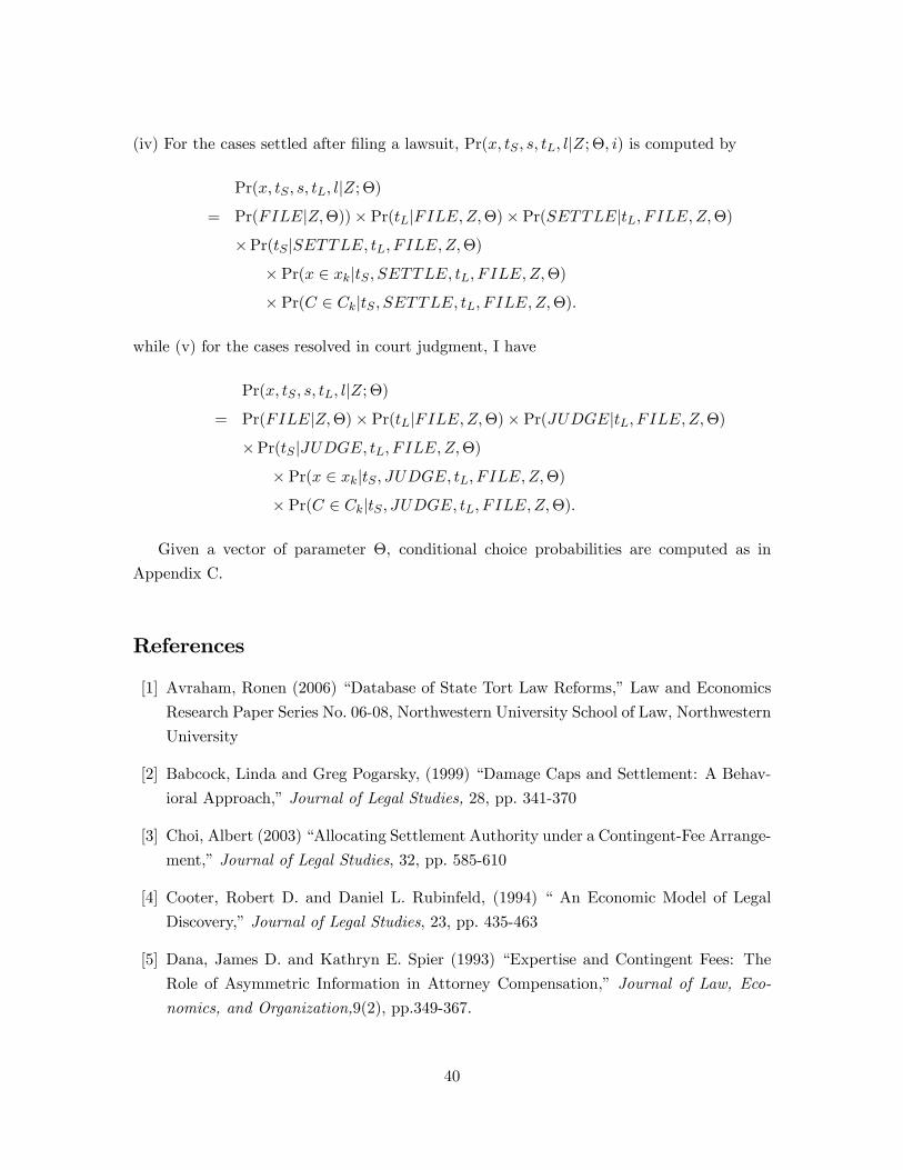
(iv) For the cases settled after �ling a lawsuit, Pr(x; tS ; s; tL; ljZ; �; i) is computed by
Pr(x; tS ; s; tL; ljZ; �)
= Pr(FILEjZ;�))� Pr(tLjFILE;Z;�)� Pr(SETTLEjtL; F ILE;Z;�)
�Pr(tS jSETTLE; tL; F ILE;Z;�)
� Pr(x 2 xkjtS ; SETTLE; tL; F ILE;Z;�)
� Pr(C 2 CkjtS ; SETTLE; tL; F ILE;Z;�):
while (v) for the cases resolved in court judgment, I have
Pr(x; tS ; s; tL; ljZ; �)
= Pr(FILEjZ;�)� Pr(tLjFILE;Z;�)� Pr(JUDGEjtL; F ILE;Z;�)
�Pr(tS jJUDGE; tL; F ILE;Z;�)
� Pr(x 2 xkjtS ; JUDGE; tL; F ILE;Z;�)
� Pr(C 2 CkjtS ; JUDGE; tL; F ILE;Z;�):
Given a vector of parameter �, conditional choice probabilities are computed as in
Appendix C.
References
[1] Avraham, Ronen (2006) �Database of State Tort Law Reforms,�Law and Economics
Research Paper Series No. 06-08, Northwestern University School of Law, Northwestern
University
[2] Babcock, Linda and Greg Pogarsky, (1999) �Damage Caps and Settlement: A Behav-
ioral Approach,�Journal of Legal Studies, 28, pp. 341-370
[3] Choi, Albert (2003) �Allocating Settlement Authority under a Contingent-Fee Arrange-
ment,�Journal of Legal Studies, 32, pp. 585-610
[4] Cooter, Robert D. and Daniel L. Rubinfeld, (1994) � An Economic Model of Legal
Discovery,�Journal of Legal Studies, 23, pp. 435-463
[5] Dana, James D. and Kathryn E. Spier (1993) �Expertise and Contingent Fees: The
Role of Asymmetric Information in Attorney Compensation,� Journal of Law, Eco-
nomics, and Organization,9(2), pp.349-367.
40

[6] Dranove (1988),
[7] Emons (1997),
[8] Eraslan, Hülya (2007) �Corporate Bankruptcy Reorganizations: Estimates from a Bar-
ganing Model,�International Economic Review, forthcoming.
[9] Farber, Henry S. and Michelle J. White, (1991) �Medical Malpractice: An Empirical
Examination of the Litigation Process,�RAND Journal of Economics, 22, pp.199-217
[10] Fenn, Paul and Neil Rickman (1999) �Delay and Settlement in Litigation,�Economic
Journal, 109, pp. 476-491
[11] Fong, Yuk-fai, (2005) �When Do Experts Cheat and Whom Do They Target?�Rand
Journal of Economics, 36(1), pp.113-130.
[12] Fournier, Gary M. and Thomas W. Zuehlke, (1996) �The timing of out-of-dourt set-
tlements,�Rand Journal of Economics, 27, pp. 310-321
[13] Gruber, Jonathan and Maria Owings (1996) �Physician Financial Incentives and Ce-
sarean Section Delivery,�Rand Journal of Economics, 27, pp. 99-123.
[14] Hay, Bruce L. (1996) �Contingent Fees and Agency Costs,�Journal of Legal Studies,
15(2), pp.503-533.
[15] Hay, Bruce L. (1997) �Optimal Contingent Fees in a World of Settlement,�Journal of
Legal Studies, 16(1), pp. 259-278
[16] Helland, Eric and Alexander Tabarrok, (2003) �Contingency Fees, Settlement Delay,
and Low-Quality Litigation: Empirical Evidence from Two Datasets,�Journal of Law,
Economics, and Organization, 19(2), pp. 517-542
[17] Hubbard, Thomas N. (1998) �An Empirical Examination of Moral Hazard in the Ve-
hicle Inspection Market,�RAND Journal of Economics, 29(2), pp. 406-426
[18] Iizuka, Toshiaki, (2006) �Experts�Agency Problems: Evidence from the Prescription
Drug Market in Japan,�RAND Journal of Economics, forthcoming.
[19] Kessler, Daniel P. (1996) �Institutional Causes of Delay in the Settlement of Legal
Disputes,�Journal of Law, Economics, and Organization, 12, pp. 432-460
[20] Kessler, Daniel P. and Daniel L. Rubinfeld (2004) �Empirical Study of the Civil Justice
System,�NBER Working Paper 10825
41

[21] Kessler, Daniel P. and Mark B. McCllelan (1996) �Do Doctors Practice Defensive
Medicine,�Quarterly Journal of Economics, Vol 111(2), pp. 353-390
[22] Kritzer, Herbert M. (1998) �Contingency-Fee Lawyers and Their Clients: Settlement
Expectations, Settlement Realities, and Issues of Control in the Lawyer-Client Rela-
tionship,�Law and Social Inquiry, 23, pp.795-821.
[23] Landes, W.M. (1971) �An Economic Analysis of the Courts,� Journal of Law and
Economics, 14, pp. 61-107
[24] Levitt, Steven D. and Chad Syverson, (2006) �Market Distortions when Agents are
Better Informed: The Value of Information in Real Estate Transactions,�mimeo, Uni-
versity of Chicago
[25] Miller, Geo¤rey P. (1987) �Some Agency Problems in Settlement,� Journal of Legal
Studies, 16(1), pp.189-215
[26] Polinsky, Mitchell A. and Daniel L. Rubinfeld (2003) �Aligning the Interests of Lawyers
and Clients,�American Law and Economics Review, 5(1), pp165-188.
[27] Posner, R (1972) �The Behavior of Administrative Agencies,�Journal of Legal Stud-
ies,1,pp. 305-347
[28] Priest, George L., and Benjamin Klein (1984) �The Selection of Disputes for Litiga-
tion,�Journal of Legal Studies, 13, pp.1-56
[29] Rickman, Neil (1999) �Contingent Fees and Litigation Settlement,� International Re-
view of Law and Economics, 19, pp.295-317.
[30] Rubinfeld, Daniel L. and Suzanne Scotchmer (1993) �Contingent Fees for Attorneys:
An Economic Analysis,�RAND Journal of Economics, 24(3), pp.343-356.
[31] Sieg, Holger (2000) �Estimating a Bargaining Model with Asymmetric Information:
Evidence from Medical Malpractice Disputes,� Journal of Political Economy, Vol
108(5), pp. 1006-1021
[32] Sloan, Frank A., Penny B. Githens, Ellen Wright Clayton, Gerald B. Hickson, Douglas
A. Gentile, and David F. Partlett (1993) Suing for Medical Malpractice, University of
Chicago Press, Chicago IL
[33] Spier, Kathryn E. (1992) �The Dynamics of Pretrial Negotiation,�Review of Economic
Studies, 59, pp. 93-108
[34] Spier, Kathryn E. (2007) �Litigation,�The Handbook of Law and Economics
42

[35] Tillinghast Towers-Perrin, (2003) U.S. Tort Costs: 2003 Update available online at
http:// www.towersperrin.com/tillinghast/publications/reports/2003_Tort_Costs_Update/Tort_Costs
_Trends_2003_Update.pdf
[36] US Congress Joint Economic Committee (2003) �Liability for Medical Malpractice:
Issues and Evidence.�Online at http://www.house.gov/jec/tort/05-06-03.pdf
[37] Waldfogel, Joel (1995) �The Selection Hypothesis and the Relationship between Trial
and Plainti¤ Victory,�Journal of Political Economy, 103, pp. 229-260
[38] Watanabe, Yasutora (2006) �Learning and Barganing in Dispute Resolution: Theory
and Evidence from Medical Malpractice Litigation,�mimeo, Northwestern University
[39] Watts, Alison (1994) �Barganinig Through an Expert Attorney,�Journal of Law, Eco-
nomics, and Organization,10(1), pp168-186.
[40] Wolinsky (1993),
[41] Wittman, Donald (1989) �Dispute Resolution, Bargaining, and the Selection of Cases
for Trial: A Study of the Generation of Biased and Unbiased Data,�Journal of Legal
Studies, 17, pp. 313-352.
[42] Yildiz, Muhamet (2003) �Bargaining Without a Common Prior - An Immediate Agree-
ment Theorem,�Econometrica, 71, pp. 793-811
[43] Yildiz, Muhamet (2004) �Waiting to Persuade,�Quarterly Journal of Economics, 119,
pp. 223-248
43