THE CAPM AND VALUE AT RISK AT DIFFERENT TIME SCALES Viviana Fernandez1

Abstract

Wavelet analysis, a refinement of Fourier analysis that was developed in the late 1980’s, is a powerful tool for decomposing time series data into orthogonal components with different frequencies. Each frequency is localized in the time domain, which makes it possible to quantify correlations between time series at different time horizons. In this article, we focus on the estimation of the capital asset pricing model (CAPM) at different time scales for Chile’s stock market. Our sample is comprised of twenty four stocks that were actively traded on the Santiago Stock Exchange over 1997–2002. We find evidence in support of the CAPM at a medium–term horizon. We extend the literature in this area to analyze the impact of time scaling on the computation of value at risk. We conclude that risk is concentrated at the higher frequencies of the data. JEL: C22, G15 Keywords: wavelet analysis, CAPM, value at risk.

1 Center for Applied Economics (CEA), Department of Industrial Engineering at the University of Chile. Postal: Avenida Republica 701, Santiago–Chile. E–mail: vfernand@dii.uchile.cl. Funds provided by an institutional grant of the Hewlett Foundation to CEA are greatly acknowledged. All remaining errors are the author’s.

2

I Introduction

The basic capital asset pricing model (CAPM), a corner-stone of modern finance, states that the risk premium of an individual asset equals its beta times the risk premium on the market portfolio. Beta measures the degree of co-movement between the asset’s return and the return on the market portfolio. In other words, beta quantifies the systematic risk of an asset––the amount of risk that cannot be diversified away. The CAPM was the result of independent work by Sharpe (1964), Lintner (1965), and Mossin (1966).

In recent years, however, the CAPM has been questioned by several empirical

studies. In particular, Fama and French (1992)’s work announced the death of beta. Using a sample for 1963-1990, they found that beta does a poor job of explaining the cross-section variation of average returns, as opposed to the book-to-market ratio and market capitalization (firm size). Kothari and Shanken (1998), however, conclude that Fama and French’s results hinge on using monthly rather than yearly returns. Kothari and Shanken argue that the use of annual returns to estimate betas helps to circumvent measurement problems caused by non-synchronous trading, seasonality in returns, and trading frictions. Based on annual returns over 1927-1990, the authors conclude that the betas are statistically significant, and that the incremental contribution of size to explaining cross-section differences in returns, beyond beta, is small.

Simultaneously, several authors have worked on theoretical extensions of the CAPM: the after-tax CAPM that accounts for the fact that investors have to pay higher taxes on high-dividend yield stocks, and, therefore, must be compensated with higher pre-tax returns; the intertemporal CAPM that deals with a multi-period setting; the consumption CAPM that states that security returns will be closely correlated with aggregate economic output, as investors are concerned with protecting their consumption over economic slowdowns; the international asset pricing model (IAPM) that establishes the conditions under which fully integrated capital markets are in equilibrium (see Megginson, 1997, for a through discussion and citations).

Another topic that has been covered in the empirical literature of the CAPM, and that it is connected with our research, is the testing of asset pricing models that allow for a time-varying beta, a time-varying risk premium, or both. This research area has received the name of tests of the conditional CAPM because the next period expected return and/or variance is routinely updated conditional on the most recent past information. Typically, the machinery used in such testing is generalized autoregressive conditional heteroscedastic (GARCH) and GARCH-in-mean (GARCH-M) processes (e.g., Engle, Lilien and Robins, 1987; Bollerslev, Engle, and Wooldridge, 1988). An alternative, but promising, approach is wavelet methods.

Wavelet analysis is a refinement of Fourier analysis that was developed in the late

1980’s, and which offers a powerful methodology for processing signals, images, and other types of data. In particular, the discrete wavelet transform allows for the decomposition of time series data into orthogonal components with different frequencies. This makes it possible to quantify correlations between markets at different time horizons. As discussed in the next sections, wavelets will allow us to estimate the CAPM for different time

3

horizons. Recent applications of wavelet methods in economics and finance are Ramsey and Lampart (1998), Norsworthy, Li and Gorener (2000), Lee (2001a, 2001b), Li and Stevenson (2001), and Gençay, Whitcher, and Selcuk (2003).

Ramsey and Lampart (1998) study the permanent income hypothesis, and conclude that time–scale decomposition is very important to analyzing economic relationships. In particular, they find that an appropriate way to model the consumption–income relationship during the post–war period is at the time scale dominated by a trend. At lower scales (i.e., higher frequencies), the degree of fit and the slope of the consumption–income relationship declines monotonically, except for the lowest scale.

Norsworthy, Li and Gorener (2000) and Gençay, Whitcher, and Selçuk (2003) apply wavelet analysis to the estimation of the CAPM. The main conclusion of Norsworthy et al. is that the major part of the market’s influence on an individual asset return is at higher frequencies. In other words, the beta coefficient will generally decrease when regressing an individual asset return on the smoother components of the market portfolio. Moreover, the R2 of such regressions will generally decline as the frequency of the market portfolio decreases.

Unlike Norsworthy et al., who model an individual asset return on different time

scales of the market portfolio, Gençay et al. focus on a portfolio and calculate the wavelet variance of the market return and the wavelet covariance between the market return and the portfolio return at each scale to obtain the corresponding portfolio beta. Their finding is that the relationship between the return on a portfolio and its beta becomes stronger as the scale increases. That is to say, the predictions of the CAPM model are more relevant at the medium-term than at short-time horizons. Lee (2001a) studies the interaction between the U.S. and the South Korean stock markets. Using the KOSPI and the DJIA, and the KOSDAQ and the NASDAQ, he finds evidence of price and volatility spillover effects from the U.S. to South Korea, but not vice versa. Lee concludes that his findings confirm the importance of innovations in developed stock markets to the determination of stock returns and volatility in emerging economies. In turn Lee (2001b) illustrates the use of wavelet analysis for seasonality filtering of time-series data. Li and Stevenson (2001) use wavelets to study the relation between futures and spot prices. They find that the lead-lag relationship between the spot and the futures index prices, well-documented in the literature, is more persistent when more detailed information is used for price reconstruction. Therefore, if the non-contemporaneous relationship between the spot and the futures indices is due to market imperfections, investors should concentrate exclusively on those imperfections that are likely to take place in the very short run.

Further discussion of the use of wavelets in economics and finance can be found in Ramsey (2002).

4

This article is organized as follows. Section II presents a brief theoretical background on the CAPM and wavelets. Section III shows our estimation results for the CAPM and value at risk at different time scales, using a sample of firms that traded actively on the Santiago Stock Exchange over 1997-2002. Finally, Section IV presents our main conclusions. II Theoretical Background 2.1 A Market Equilibrium Model: The CAPM

The capital asset pricing model states that the equilibrium rate of return on all risky assets is a function of their covariance with the market portfolio. The derivation of the CAPM equation is based upon the assumptions of risk-averse investors, frictionless markets, absence of information costs and information asymmetries, unlimited borrowing and lending at the risk-free rate, and perfect divisibility and marketability of financial assets (see, for instance, Copeland, Weston, and Shastri, 2004; Megginson, 1997). The CAPM establishes that the expected return on any risky satisfy the equation: )RR(ER)R(E fmifi −β+= , (1) where Ri is the return on asset i, Rf is the risk-free rate, Rm is the return on the market

portfolio, and )R(Var

)R,R(Cov

m

mii =β is the asset’s beta.

The (E(Rm)–Rf) term is referred to as the market risk premium, given that it represents the return over the risk-free rate required by investors to hold the market portfolio. Equation (1) can be re-written as )RR(ER)R(E fmifi −β=− . (2) This says that the risk premium on an individual asset equals its beta time the market risk premium. The empirical version of equation (2) is given by ifmiifi )RR(RR ε+−β+α=− , (3) where εi is a random error term. From this expression, we can obtain the following relationship for the variance of the return on asset i: 22

m2i

2i εσ+σβ=σ . (4)

5

Equation (4) says the total risk of an asset (variance) can be partitioned into systematic risk (a measure of how the asset covariates with the economy), 2

m2i σβ , and unsystematic risk

(independent of the economy), 2εσ .

2.2 Wavelet Analysis in a Nutshell Wavelets or short waves are similar to sine and cosine functions in that they also oscillates about zero. However, as its name indicates, oscillations of a wavelet fade away around zero, and the function is localized in time or space.2 In wavelet analysis, a signal (i.e., a sequence of numerical measurements) is represented as a linear combination of wavelet functions. Unlike Fourier series, wavelets are suitable building-block functions for signals whose features change over time, and for non-smooth signals. A wavelet allows for decomposing a signal into multi–resolution components: fine and coarse resolution components. There are father wavelets φ and mother wavelets ψ such that ∫ =φ 1dt)t( ∫ =ψ 0dt)t( . (1) Father wavelets are good at representing the smooth and low-frequency parts of a signal, whereas mother wavelets are good at representing the detailed and high-frequency parts of a signal. The most commonly used wavelets are the orthogonal ones (i.e., haar, daublets, symmelets, and coiflets). In particular, the orthogonal wavelet series approximation to a continuous signal f(t) is given by )t(d...)t(d)t(d)t(s)t(f k,1

kk,1k,1J

kk,1Jk,J

kk,Jk,J

kk,J ψ++ψ+ψ+φ≈ ∑∑∑∑ −− , (2)

where J is the number of multi-resolution components or scales, and k ranges from 1 to the number of coefficients in the corresponding component. The coefficients sJ,k, dJ,k,..., d1,k are the wavelet transform coefficients, whereas the functions φj,k(t) and ψj,k(t) are the approximating wavelet functions. These functions are generated from φ and ψ as follows

⎟⎟⎠

⎞⎜⎜⎝

⎛ −φ=φ −

j

j2/j

k,j 2k2t2)t( ⎟⎟

⎠

⎞⎜⎜⎝

⎛ −ψ=ψ −

j

j2/j

k,j 2k2t2)t( . (3)

The wavelet coefficients can be approximated by the following integrals ∫ φ≈ dt)t(f)t(s k,Jk,J ∫ ψ≈ dt)t(f)t(d k,jk,j , j=1, 2, ..., J. (4)

2 Mathematically, a function ϖ(.) defined over the entire real axis is called a wavelet if ϖ(t)→0 as t→±∞.

6

These coefficients are a measure of the contribution of the corresponding wavelet function to the total signal. On the other hand, the approximating wavelet functions φj,k(t) and ψj,k(t) are scaled and translated versions of φ and ψ. As equation (3) indicates, the scale or dilation factor is 2j, whereas the translation or location parameter is 2jk. As j gets larger, so does the scale factor 2j, and the functions φj,k(t) and ψj,k(t) get shorter and more spread out. In other words, 2j is a measure of the width of the functions φj,k(t) and ψj,k(t). Likewise, as j increases, the translation step gets correspondingly larger in order to match the scale parameter 2j. Most applications of wavelet analysis make use of a discrete wavelet transform (DWT). The DWT calculates the coefficients of the approximation in (2) for a discrete signal of final extent, f1, f2,.., fn. That is, it maps the vector f=(f1, f2,…,fn)′ to a vector ω of n wavelet coefficients that contains sJ,k and dj,k, j=1,2,…, J. The sJ,k are called the smooth coefficients and the dj,k are called the detail coefficients. Intuitively, the smooth coefficients represent the underlying smooth behavior of the data at the coarse scale 2J, whereas the detail coefficients provide the coarse scale deviations from it. When the length of the data n is divisible by 2J, there are n/2 coefficients d1,k at the finest scale 21=2. At the next finest scale, there are n/22 coefficients d2,k. Similarly, at the coarsest scale, there are n/2J dJ,k coefficients and n/2J sJ,k coefficients. Altogether, there are

n21

21

n J

J

1ii =⎟⎟

⎠

⎞⎜⎜⎝

⎛+∑

=

coefficients. The number of coefficients at a given scale is related to the

width of the wavelet function. For instance, at the finest scale, it takes n/2 terms for the functions ψ1,k(t) to cover the interval 1≤t≤n. The wavelet coefficients are ordered from coarse scales to fine scales in the vector ω. If n is divisible by 2J, ω will be given by

⎟⎟⎟⎟⎟⎟

⎠

⎞

⎜⎜⎜⎜⎜⎜

⎝

⎛

= −

1

1J

J

d

dds

ω

J

M

, (5)

where

)'d,...,d,d(

)'d,...,d,d()'d,...,d,d()'s,...,s,s(

2/n,12,11,11

2/n,1J2,1J1,1J1J

2/n,J2,J1,JJ

2/n,J2,J1,JJ

1J

J

J

=

===

−−−−−

d

dds

MM

7

Each of the sets of coefficients sJ, dJ,…,d1 is called a crystal. Expression (2) can be rewritten as f(t) ≈ SJ(t)+DJ(t)+DJ–1(t)+...+D1(t), (6) where )t(s)t(S k,J

kk,JJ φ=∑ (7a)

)t(d)t(D k,Jk

k,jJ ψ=∑ (7b)

are denominated the smooth signal and the detail signals, respectively. The terms in expression (6) represent a decomposition of the signal into orthogonal signal components SJ(t), DJ(t), DJ–1(t), ...,D1(t) at different scales. These terms are components of the signal at different resolutions. That is why the approximation in (6) is called a multi-resolution decomposition (MRD). 2.3 Computation of Wavelet Variance and Covariance Wavelet variance analysis consists in partitioning the variance of a time series into pieces that are associated to different time scales. It tells us what scales are important contributors to the overall variability of a series (see Percival and Walden, 2000). In particular, let x1, x2,..., xn be a time series of interest, which is assumed to be a realization of a stationary process with variance 2

Xσ . If )( j2X τυ denotes the wavelet variance for scale

τj≡2j−1, then the following relationship holds:

)( j1j

2x

2X τυ=σ ∑

∞

=

(8)

This relationship is analogous to that between the variance of a stationary process and its spectral density function (SDF):

df)f(S2/1

2/1X

2X ∫

−

=σ (9)

where SX(f) is the SDF at the frequency f ∈ [–1/2, 1/2]. The SDF for a stationary process decomposes the variance across different frequencies, whereas the wavelet variance decomposes it across different scales. Given that the scale τj can be related to range of frequencies in the interval [1/2j, 1/2j–1], the wavelet variance usually leads to a more succinct decomposition. Moreover, unlike the SDF, the square root of the wavelet variance is expressed in the same units as the original data.

8

Another advantage of the wavelet variance is that it replaces the sample variance with a sequence of variances over given scales. That is, it offers a scale–by–scale decomposition of variability, which makes it possible to analyze a process that exhibits fluctuations over a range of different scales. Let ⎣ ⎦jj 2/nn =′ be the number of discrete wavelet transform (DWT) coefficients at

level j, where n is the sample size, and ⎥⎥⎤

⎢⎢⎡ −−≡′ )

211)(2L(L jj be the number of DWT

boundary coefficients3 at level j (provided that jj Ln ′>′ ), where L is the width of the wavelet filter4. An unbiased estimator of the wavelet variance is defined as

∑−′

−′=′−′≡τυ

1n

1Lt

2t,jj

jjj

2X

j

j

d2)Ln(

1)(ˆ (10)

Given that the DWT decorrelates the data, the non-boundary wavelet coefficients in a given level (dj) are zero–mean Gaussian white noise process. Similarly, the unbiased wavelet covariance between the time series X and Y, at scale j, can be defined as

)Y(t,j

1n

Lt

)X(t,jj

jjj

2XY dd

2)Ln(1)(ˆ

j

j

∑−′

′=′−′≡τυ (11)

provided that jj Ln ′>′ . In the CAPM model, as proposed by Gençay, Whitcher and Selçuk (2003), the wavelet beta estimator for asset i, at scale j, is defined as

)(ˆ)(ˆ

)(ˆj

2R

j2

RRji

m

mi

τυ

τυ=τβ (12)

where )(ˆ j

2RR mi

τυ is the wavelet covariance of asset i and the market portfolio at scale j, and

)(ˆ j2R m

τυ is the wavelet variance of the market portfolio at scale j.

3 ⎣ ⎦x and ⎡ ⎤x represent the greatest integer ≤x and the smallest integer x≥, respectively. Boundary coefficients are those that are formed by combining together some values from the beginning of the sequence of scaling coefficients with some values from the end. 4 In practical applications, we deal with sequences of values (i.e., time series) rather than functions defined over the entire real axis. Therefore, instead of using actual wavelets, we work with short sequences of values named wavelet filters. The number of values in the sequence is called the width of the wavelet filter, and it is denoted by L.

9

III Data and Estimation Results In this section, we focus on estimating the CAPM at different time scales for a group of stocks regularly traded on the Santiago Stock Exchange. We selected those stocks that were traded at least 85 percent of all business days over the sample period (January 1997-Sepetmber 2002). Table 1 presents descriptive statistics of excess returns on the 24 stocks in the sample and on the proxy for the market portfolio, the Price Index of Selected Stocks (IPSA). The latter gathers the 40 most actively-traded stocks on the Santiago Stock Exchange over the past year. The risk-free rate of return is proxied by the 30-day nominal interest paid on bank deposits. This choice is based on data availability of interest rates at a daily frequency, and on the fact that longer-maturity interest rates are inflation indexed. Given that we work with nominal returns, we use a nominal proxy for the risk-free rate.

[Table 1] The figures in Table 1 show that, as is the case with most financial assets, excess returns on the stocks and the market portfolio exhibit little skewness but high excess kurtosis. The next step consists of running some exploratory regressions to study the relationship between the excess return on each individual stock and the time scales of the market portfolio. In particular, we estimate a linear regression of each stock excess return (Ri–Rf) on each recomposed crystal j of the market portfolio (Rm–Rf)j: j

ijmi

ji

ji

jfm

ji

jifi D)RR(RR ε+β+α≡ε+−β+α=− j=1, 2,.., 6. (13)

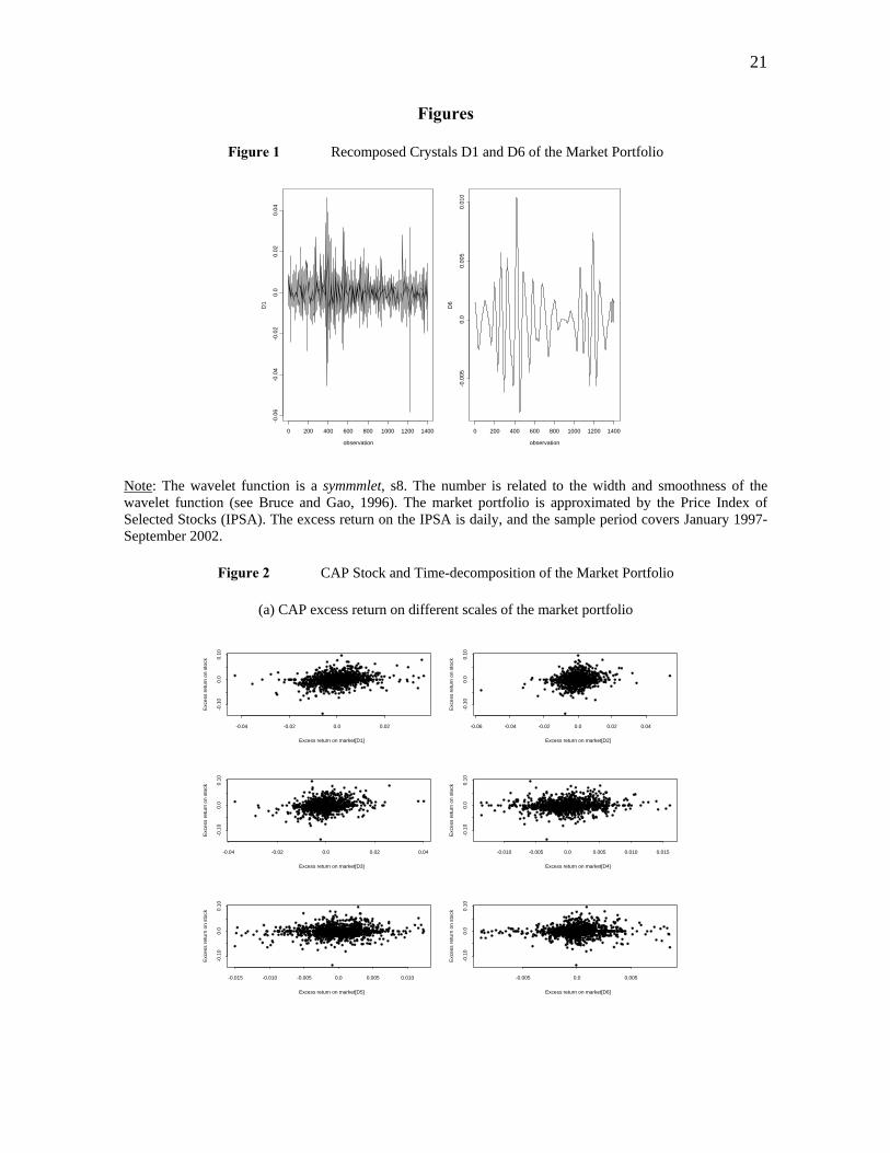
Given that we work with daily data, wavelet scales are such that scale 1 is associated with 2-4 day dynamics, scale 2 with 4-8 day dynamics, scale 3 with 8-16 day dynamics, scale 4 with 16-32 day dynamics, scale 5 with 32-64 day dynamics, and scale 6 with 64-128 day dynamics. Scale 7 corresponds with 128-256 day dynamics, that is, approximately one year. The linear model in (13) is estimated up to scale 6 of the market portfolio because scale 7 includes not only D7 but also S7. Therefore, when recomposing the market excess returns at scale 7, we cannot separate D7 from S7. For illustrative purposes, Figure 1 shows the recomposed crystals D1 and D6 of the excess return on the market portfolio at scales 1 and 6, respectively. As we see, D1 depicts the high frequency movements of the market portfolio, whereas D6 depicts its long-term behavior.

[Figure 1] Table 2 reports the regression results. When looking at individual excess returns, the mean contribution of j

mD tends to decline as the scale increases, and so does its explanatory power measured by R2. This implies that the major part of the market portfolio’s influence on individual stocks is at higher frequencies (i.e., lower scales). Put another way, the systematic-risk component of the excess returns on individuals stocks is captured to greater extent by the detailed components of the market portfolio.

10

[Table 2]

An alternative way of analyzing the same issue is by regressing each individual excess return on the recomposed residues of the market portfolio. The residue of the market

portfolio at scale j is defined as ∑=

−=j

1i

imm

jm DRS , j=1, …, 6. By construction, as the scale

increases, the variation of the market portfolio left out in the recomposed residue decreases. And, in consequence, the fraction of systematic risk of each stock explained by the recomposed residue of the market portfolio falls monotonically with frequency, on average (Table 3). Similar conclusions are drawn by Nortsworthy, Li and Gorener (2000) for a sample of 99 stocks of the S&P 500 in 1998.

[Table 3]

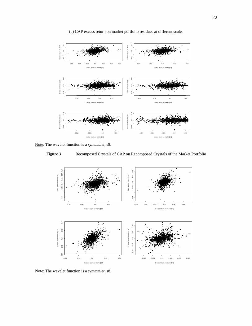
Our above findings can be visualized in Figure 2, for the particular case of the CAP stock. Panel (a) shows the CAP excess return on scales 1 to 6 of the market portfolio. As the frequency of the excess return on the market portfolio declines, the relationship between the two variables departures more from linearity. A similar pattern is observed in Panel (b), where the CAP excess return is plotted against scales 1 to 6 of the market portfolio residues.

[Figure 2] Strictly speaking, j

iβ in equation (13) is not a true beta because the excess returns on the individual stock and the market portfolio are measured at different time scales. Therefore, a more accurate measure of beta, at scale j, is given by expression (12). Table 4 shows our estimation results. We also report an R2 for each scale, which is computed as

)(ˆ)(ˆ

)(ˆ)(Rj

2R

j2R2

jij2i

i

m

τυ

τυτβ=τ (14)

[Table 4]

Unlike the results reported in Tables 2 and 3, the linear relationship between the excess return and the market portfolio becomes in general stronger at higher scales of the two variables. This is illustrated in Figure 3, where each recomposed crystal of the excess return on the CAP stock is plotted on the corresponding recomposed crystal of the market portfolio. The linear association between the two variables is particularly strong at scales 2 and 3. This evidence implies that the fraction of systematic risk contained in an individual stock at lower frequencies has a higher association with lower frequencies of the market portfolio.

[Figure 3] The betas reported in Table 4 allow us to compute an average market premium at each time scale. Specifically, we run a regression on the average risk premium of each stock fi RR − on its wavelet beta estimate at scale j, )(ˆ

ji τβ . The regression is also

11

estimated for the betas obtained from the raw data. Table 5 reports the ordinary least-squared estimates, whereas Figure 4 shows the average risk premium for each of the 24 stocks in the sample on its corresponding beta at scales 1 to 6.

[Table 5, Figure 4]

From the sample, the average market premium was –9.06 percent per year. The slope estimate at scale 2, which is statistically significant at the 10 percent level, is the one closest to this figure: –11.5 percent per year. At scales 4 to 6, the relationship between the average risk premium and the wavelet beta of each stock is statistically insignificant. Meanwhile, the first row of Table 5 shows that the average market premium yielded by the raw data (–13.7 percent per year) underestimates the sample average market premium. These results, along with those reported in Table 4, indicate that the CAPM model tends to be more statistically significant at scales 2 and 3 of data. In other words, its predictions are more meaningful for investment horizons of 4-16 days. IV An application to Value at Risk From the CAPM, ifmiifi )RR(RR ε+−β+α=− . k=1, 2,...,k. (15) Then, the variance of the excess return i and the covariance between the excess returns i and j are given, respectively, by 22

m2i

2i εσ+σβ=σ , i=1, 2,..,k,

2

mjiij σββ=σ , where 22

i i)(E εσ=ε and E(εiεj)=0, ∀i≠j.

Consequently, the variance-covariance matrix of excess returns is given by EββΩ +σ= 2

m' (16)

where

⎟⎟⎟⎟⎟

⎠

⎞

⎜⎜⎜⎜⎜

⎝

⎛

β

ββ

=

k

2

1

Mβ and

⎟⎟⎟⎟⎟

⎠

⎞

⎜⎜⎜⎜⎜

⎝

⎛

σ

σσ

=

ε

ε

ε

2

2

2

k

2

1

00

0000

K

MOMM

L

L

E .

The (1–α) %-value at risk (VaR) of a portfolio of k assets is then ωEββω )'(')(lV)(VaR 2

m0 +σα=α (17)

12

where ω is a k x 1 vector of portfolio weights, V0 is the initial value of the portfolio, and l(α)=Φ−1(1−α), where Φ(.) is the cumulative distribution function of the standard normal. For an equally-weighted portfolio, ωi=1/k, ∀ i, the VaR boils down to

∑∑=

ε=

σ+⎟⎠

⎞⎜⎝

⎛βσα=α

k

1i

22

2k

1ii

2m0 ik

1k/)(lV)(VaR . (18)

As k becomes large, 2k

1ii

2m0 k/)(lV)(VaR ⎟

⎠

⎞⎜⎝

⎛βσα≈α ∑

=

. That is, for a well-

diversified portfolio, all that matters to computing VaR is systematic risk. We use equation (18) to compute the value at risk at different time scales. In particular, the VaR at scale j can be obtained by evaluating (18) at the j-scale components of the variance of the market portfolio return, the betas of the k stocks, and of the variances of the error terms that capture non-systematic risk.

∑∑=

ε=

τ τσ+⎟⎠

⎞⎜⎝

⎛τβτσα=α

k

1ij

22

2k

1ijij

2m0 )(

k1k/)()()(lV)(VaR

ij. (19)

In order to obtain )( j

2iτσε , we use the relation )()()()( j

2j

2mj

2ij

2i τσ+τστβ=τσ ε .

That is, )()()()( j

2mj

2ij

2ij

2 τστβ−τσ=τσε (20) The variance of stock i at scale j, )( j

2i τσ , the beta of stock i return at scale j, )( ji τβ , and

the variance of the market portfolio at scale j, )( j2m τσ , can be computed using equations

(10) and (12). Now it should be the case that

∑ ∑∑−

= =ε

= ⎟⎟⎠

⎞⎜⎜⎝

⎛τσ+⎟

⎠

⎞⎜⎝

⎛τβτσα≈α

1J

1j

k

1ij

22

2k

1ijij

2m0 )(

k1k/)()()(lV)(VaR

i (21)

The right-hand side of (21) is an approximation to the VaR of the raw data (equation

(18)) because we do not have a beta estimate for the highest scale J. However, the rounded error should be negligible, in general, as most energy is concentrated at the lower scales.5 5 The energy in a given crystal is calculated as the sum of squares of all of its elements over the sum of squares of all observations in the original time series. One appealing characteristic of the discrete wavelet

13

From expressions (18) and (21), we have

∑∑

∑ ∑∑

=ε

=

−

= =ε

=

σ+⎟⎠

⎞⎜⎝

⎛βσ

τσ+⎟⎠

⎞⎜⎝

⎛τβτσ

≈k

1i

22

2k

1ii

2m

1J

1j

k

1ij

22

2k

1ijij

2m

i

i

k1k/

)(k1k/)()(

1 .

We can interpret the ratio

∑∑

∑∑

=ε

=

=ε

=

σ+⎟⎠

⎞⎜⎝

⎛βσ

τσ+⎟⎠

⎞⎜⎝

⎛τβτσ

k

1i

22

2k

1ii

2m

k

1ij

22

2k

1ijij

2m

i

i

k1k/

)(k1k/)()(

(22)

as the contribution of scale j to total value at risk. Table 6 shows our computations. First, as expected, value at risk generally decreases as the time scale increases. Second, the contribution to total risk is higher at the lower scales. That is to say, potential portfolio losses at a 1-day horizon are larger when looking at the detailed components of the data. Finally, the last two rows of the table show the value at risk computed by equations (18) and (21), respectively. As we see, the discrepancy between the two figures shows up only at the fifth decimal.

[Table 6] IV Conclusions

The basic capital asset pricing model (CAPM) states that the risk premium of an individual asset equals its beta times the risk premium on the market portfolio. Beta measures the degree of co-movement between the asset’s return and the return on the market portfolio. In recent years, however, the CAPM has been questioned by several empirical studies.

One strand of the literature has built asset pricing models that allow for a time-

varying beta, a time-varying risk premium on the market portfolio, or both. This research area has received the name of tests of the conditional CAPM because the next period expected return and/or variance is updated conditional on the most recent past information. Typically, such testing resorts to GARCH and GARCH-in-mean processes. An alternative approach is wavelet analysis, which is a refinement of Fourier analysis. Wavelets are a

transform (DWT) is that it is an energy preserving transform. This means that the energy in all the DWT coefficients equals the energy in the original time series. For instance, for the excess return on the IPSA, the first three crystals d1, d2, and d3 concentrate altogether 79 percent of the total energy, whereas crystals d1 to d6 concentrate approximately 98 percent of the total energy.

14

powerful tool for decomposing time series data into orthogonal components with different frequencies. Each frequency is localized in the time domain, which makes it possible to quantify correlations between time series at different time horizons. In this article, we focus on the estimation of the CAPM at different time scales for Chile’s stock market. Our sample is comprised of twenty four stocks that were actively traded on the Santiago Stock Exchange over 1997–2002. We find evidence in support of the CAPM at a medium–term horizon. We extend the literature in this area to analyze the impact of time scaling on the computation of value at risk. We conclude that risk is concentrated at the higher frequencies of the data. References Bollerslev, T., R. Engle, and J. Wooldridge (1988), “A Capital-Asset Pricing Model with Time-Varying Covariances,” Journal of Political Economy 96, 116-131. Bruce A. and H. Gao (1996), Applied Wavelet Analysis with S–Plus. Springer–Verlag. Copeland, T., J. Weston, and K. Shastri (2004), Financial Theory and Corporate Policy. Fourth edition. Pearson Addison Wesley. Engle R., Lilien, D., Robins, R (1987), “Estimating Time-Varying Risk Premia in the Term Structure: the ARCH-M Model”. Econometrica 55, 391-407. Fama, E. and K. French (1992), “The Cross-section of Expected Returns.” Journal of Finance 47, 427-465. Gençay R., B. Whitcher, and F. Selçuk (2003), “Systematic Risk and Time Scales.” Quantitative Finance 3, 108-116. Kothari, S., and J. Shanken (1998), “On defense of beta.” The Revolution in Corporate Finance, J. Stern and D. Chew, editors. Third edition, 52-57. Megginson, W. (1997), Corporate Finance Theory. Addison-Wesley Educational Publishers Inc. Mossin, I. (1966), “Equilibrium in a Capital Asset Market.” Econometrica 34, 768-783. Lee, Hahn Shik (2001a), “Price and Volatility Spillovers in Stock Markets: A Wavelet Analysis”. Manuscript presented at the 2001 Australasian Meeting of the Econometric Society. _____________ (2001b), “Recent Advances in Wavelet Methods for Economic Time Series,” Journal of Economic Theory and Econometrics 7(1), 43–65. Lin, Shinn-Juh and M. Stevenson (2001), "Wavelet Analysis of the Cost-of-Carry Model", Studies in Nonlinear Dynamics & Econometrics 5(1), 87-102.

15

Lintner, J. (1965), “The Valuation of Risk Assets and the Selection of Risky Investments in Stock Portfolios and Capital Budgets,” Review of Economics and Statistics 47, 13-57. Norsworthy J., D. Li and R. Gorener (2000), “Wavelet–Based Analysis of Time Series: An Export from Engineering to Finance.” Manuscript presented at the 2000 IEEE International Engineering Management Society Conference. Percival, D., and A. Walden (2000), Wavelets Analysis for Time Series Analysis. Cambridge University Press, Cambridge, U.K. Ramsey J., and C. Lampart (1998), “The Decomposition of Economic Relationships by Time Scale Using Wavelets: Expenditure and Income,” Studies in Nonlinear Dynamics & Econometrics 3(1), 23–42. Ramsey, J. (2002), “Wavelets in Economics and Finance: Past and Future.” Studies in Nonlinear Dynamics & Econometrics 6(3), 1-29. Sharpe, W. (1964), “Capital Asset Prices: A Theory of Market Equilibrium under Conditions of Risk. “ Journal of Finance 19, 425-442.

16

Tables

Table 1 Descriptive statistics of excess returns

Stock Trading days

Average Median Std. Dev. 1st quartile 3rd-quartile Excess Kurtosis

BESALCO 89% –0.001 0.000 0.023 –0.007 0.000 16.8 CAP 95% –0.001 0.000 0.020 –0.011 0.008 3.9 CERVEZAS 88% 0.000 0.000 0.022 –0.007 0.007 13.0 CGE 93% –0.001 0.000 0.029 –0.015 0.010 2.8 CMPC 100% 0.000 0.000 0.015 –0.008 0.006 2.3 COLBUN 99% 0.000 0.000 0.022 –0.001 0.000 3.0 COPEC 100% 0.000 0.000 0.018 –0.009 0.009 2.8 CTC–A 100% –0.001 0.000 0.021 –0.012 0.009 5.7 CUPRUM 96% 0.000 0.000 0.019 –0.006 0.006 7.2 CHILECTRA 92% –0.001 0.000 0.017 –0.008 0.005 7.0 D&S 98% 0.000 0.000 0.024 –0.010 0.010 12.7 ENDESA 100% –0.001 0.000 0.019 –0.010 0.009 8.5 ENERSIS 100% –0.001 0.000 0.021 –0.011 0.009 4.1 ENTEL 100% 0.000 0.000 0.020 –0.011 0.009 3.1 FALABELLA 99% 0.000 0.000 0.019 –0.010 0.009 4.9 GASCO 89% 0.000 0.000 0.017 –0.002 0.003 5.1 IANSA 99% –0.001 0.000 0.025 –0.015 0.003 3.5 LAN 86% 0.000 –0.001 0.014 –0.007 0.006 6.3 MASISA 94% –0.001 0.000 0.022 –0.010 0.009 3.9 ORO BLANCO 93% –0.001 0.000 0.029 –0.015 0.010 2.8 PARIS 93% 0.000 0.000 0.019 –0.010 0.007 6.4 SAN PEDRO 98% 0.000 0.000 0.016 –0.006 0.007 5.1 SM–CHILE B 97% 0.000 0.000 0.022 –0.001 0.000 14.1 SQM–B 89% –0.001 0.000 0.023 –0.010 0.009 34.8 IPSA (Market) 100% 0.000 –0.001 0.013 –0.007 0.006 6.2

Notes: (1) The data source is the Santiago Stock Exchange. The sample period is January 1997-September 2002, and returns are daily. (2) Trading days represent the percentage of business days over the sample period on which the stock was traded. (3) IPSA is a proxy for the market portfolio. It gathers the forty stocks that were most actively traded over the past year. (4) The proxy for the risk-free rate is the interest rate paid on 30-day deposits.

17

Table 2 Individual Excess Returns on the Recomposed Crystals of the Market Portfolio

Beta R2

Stock D1 D2 D3 D4 D5 D6 D1 D2 D3 D4 D5 D6 BESALCO 0.318 0.228 0.225 0.712 0.311 1.615 0.019 0.005 0.002 0.011 0.002 0.033 CAP 0.592 0.560 0.747 0.515 0.681 0.690 0.054 0.037 0.054 0.009 0.015 0.005 CERVEZAS 0.245 0.679 0.992 1.014 0.832 0.642 0.009 0.045 0.064 0.035 0.025 0.003 CGE 0.153 0.141 0.246 0.323 0.694 0.530 0.010 0.004 0.012 0.009 0.028 0.012 CMPC 0.525 0.558 0.814 0.488 0.510 1.084 0.067 0.062 0.068 0.016 0.009 0.030 COLBUN 0.598 0.497 0.515 0.412 0.450 0.773 0.053 0.021 0.014 0.006 0.005 0.007 COPEC 0.924 0.826 0.955 0.709 0.734 1.112 0.155 0.100 0.069 0.024 0.014 0.026 CTC–A 1.208 1.383 1.383 1.267 1.236 1.033 0.192 0.203 0.105 0.056 0.028 0.016 CUPRUM 0.251 0.515 0.427 0.837 1.005 0.667 0.010 0.036 0.015 0.031 0.034 0.006 CHILECTRA 0.723 0.734 0.928 0.799 0.938 0.762 0.123 0.098 0.073 0.043 0.024 0.013 D&S 1.008 0.826 0.884 1.118 1.328 1.186 0.114 0.054 0.037 0.031 0.033 0.015 ENDESA 1.200 1.227 1.062 0.975 1.183 1.089 0.212 0.204 0.078 0.037 0.033 0.020 ENERSIS 1.276 1.200 1.135 1.172 1.206 0.943 0.213 0.173 0.079 0.047 0.030 0.013 ENTEL 0.741 0.769 0.750 0.842 0.717 0.871 0.081 0.072 0.036 0.026 0.013 0.010 FALABELLA 0.758 0.733 0.738 0.721 0.960 1.063 0.099 0.065 0.037 0.020 0.031 0.014 GASCO 0.160 0.267 0.284 0.422 0.771 0.604 0.006 0.013 0.009 0.009 0.028 0.008 IANSA 0.881 0.966 0.976 1.061 0.656 1.001 0.076 0.067 0.036 0.032 0.007 0.009 LAN 0.200 0.266 0.739 0.755 0.934 2.100 0.004 0.004 0.019 0.014 0.013 0.034 MASISA 0.519 0.460 0.727 1.065 1.095 1.444 0.043 0.019 0.032 0.031 0.033 0.015 ORO BLANCO 0.585 0.711 0.766 0.799 0.478 0.980 0.028 0.031 0.021 0.009 0.003 0.006 PARIS 0.513 0.743 0.783 0.669 1.088 0.999 0.048 0.073 0.044 0.022 0.043 0.011 SAN PEDRO 0.243 0.425 0.543 0.293 0.590 0.855 0.016 0.032 0.037 0.004 0.014 0.017 SM–CHILE B 0.361 0.171 0.103 0.445 0.576 0.329 0.018 0.003 0.001 0.006 0.008 0.001 SQM–B 0.827 0.978 1.052 0.902 0.994 1.078 0.079 0.100 0.057 0.022 0.020 0.017

Mean 0.617 0.661 0.741 0.763 0.832 0.977 0.072 0.063 0.042 0.023 0.021 0.014 Std. Dev 0.344 0.335 0.317 0.278 0.277 0.371 0.066 0.059 0.028 0.014 0.012 0.009

Notes: (1) Scale 1: 2-4 days, scale 2: 4-8 days, scale 3: 8-16 days, scale 4: 16-32 days, scale 5: 32-64 days, and scale 6: 64-128 days.(2) D1 is the recomposed crystal of the market portfolio at scale 1, etc. The betas are obtained by running a regression of the individual stock excess return on the recomposed crystal of the market portfolio.

18

Table 3 Individual Excess Returns on the Recomposed Residues of the Market Portfolio

Beta R2 Stock S1 S2 S3 S4 S5 S6 S1 S2 S3 S4 S5 S6

BESALCO 0.414 0.577 0.816 0.865 1.506 1.341 0.036 0.038 0.045 0.034 0.048 0.015 CAP 0.657 0.721 0.693 0.803 1.006 1.359 0.129 0.094 0.040 0.033 0.020 0.017 CERVEZAS 0.839 0.945 0.908 0.836 0.846 1.041 0.173 0.132 0.069 0.035 0.009 0.007 CGE 0.298 0.384 0.507 0.629 0.577 0.654 0.056 0.060 0.055 0.051 0.024 0.011 CMPC 0.647 0.718 0.651 0.795 1.039 0.968 0.186 0.127 0.061 0.048 0.044 0.015 COLBUN 0.506 0.513 0.511 0.597 0.787 0.809 0.055 0.034 0.020 0.014 0.011 0.004 COPEC 0.857 0.883 0.830 0.933 1.097 1.068 0.240 0.141 0.072 0.049 0.037 0.012 CTC–A 1.312 1.255 1.162 1.073 0.938 0.743 0.408 0.206 0.102 0.047 0.020 0.004 CUPRUM 0.615 0.690 0.902 0.953 0.873 1.153 0.119 0.085 0.081 0.051 0.017 0.012 CHILECTRA 0.803 0.861 0.817 0.838 0.760 0.757 0.255 0.159 0.086 0.043 0.020 0.006 D&S 0.960 1.059 1.197 1.254 1.166 1.125 0.171 0.119 0.085 0.055 0.022 0.006 ENDESA 1.138 1.061 1.061 1.130 1.081 1.065 0.378 0.176 0.098 0.062 0.029 0.010 ENERSIS 1.158 1.122 1.112 1.063 0.931 0.908 0.348 0.175 0.096 0.049 0.019 0.006 ENTEL 0.804 0.833 0.898 0.942 1.211 1.806 0.174 0.103 0.068 0.042 0.031 0.025 FALABELLA 0.796 0.844 0.918 1.056 1.194 1.344 0.180 0.116 0.081 0.063 0.033 0.019 GASCO 0.375 0.455 0.603 0.718 0.648 0.731 0.062 0.052 0.049 0.043 0.015 0.007 IANSA 0.957 0.950 0.932 0.811 0.990 0.969 0.153 0.086 0.050 0.019 0.013 0.005 LAN 0.694 0.976 1.140 1.485 2.118 2.148 0.069 0.082 0.066 0.059 0.056 0.022 MASISA 0.757 0.959 1.158 1.220 1.448 1.451 0.126 0.120 0.094 0.063 0.031 0.016 ORO BLANCO 0.727 0.739 0.716 0.668 0.936 0.863 0.073 0.042 0.021 0.012 0.009 0.003 PARIS 0.802 0.846 0.889 1.077 1.059 1.129 0.200 0.128 0.085 0.067 0.024 0.012 SAN PEDRO 0.497 0.548 0.553 0.714 0.854 0.850 0.105 0.075 0.037 0.038 0.026 0.009 SM–CHILE B 0.249 0.316 0.488 0.517 0.447 0.654 0.016 0.013 0.018 0.012 0.004 0.003 SQM–B 0.990 1.000 0.961 0.999 1.004 0.861 0.221 0.120 0.063 0.041 0.022 0.005

Mean 0.744 0.802 0.851 0.916 1.022 1.075 0.164 0.103 0.064 0.043 0.024 0.011 Std. Dev 0.270 0.242 0.223 0.230 0.337 0.362 0.106 0.049 0.025 0.016 0.013 0.006

Notes: (1) Scale 1: 2-4 days, scale 2: 4-8 days, scale 3: 8-16 days, scale 4: 16-32 days, scale 5: 32-64 days,

and scale 6: 64-128 days. (2) The recomposed residues are computed as ∑=

−=j

1i

imm

jm DRS , where j

mD is the

recomposed crystal of the market portfolio at scale j.

19

Table 4 Beta computed from Recomposed Crystals of Individual Stocks and the Market Portfolio

Beta for each scale R2 for each scale Stock 1 2 3 4 5 6 1 2 3 4 5 6

BESALCO 0.281 0.230 0.400 0.535 0.684 1.494 0.036 0.025 0.049 0.075 0.200 0.364 CAP 0.554 0.607 0.773 0.736 0.577 0.721 0.121 0.170 0.316 0.277 0.284 0.296 CERVEZAS 0.283 0.628 0.931 1.074 0.926 1.058 0.032 0.151 0.328 0.346 0.553 0.565 CGE 0.116 0.222 0.231 0.282 0.612 0.486 0.012 0.058 0.077 0.080 0.354 0.288 CMPC 0.516 0.577 0.733 0.549 0.754 0.841 0.168 0.246 0.356 0.246 0.400 0.560 COLBUN 0.600 0.480 0.574 0.459 0.471 0.508 0.087 0.089 0.182 0.147 0.185 0.464 COPEC 0.894 0.846 0.937 0.779 0.872 1.037 0.354 0.388 0.423 0.392 0.513 0.670 CTC–A 1.259 1.358 1.355 1.209 1.330 1.084 0.551 0.613 0.649 0.663 0.802 0.781 CUPRUM 0.298 0.417 0.562 0.893 0.914 1.019 0.038 0.105 0.151 0.264 0.373 0.566 CHILECTRA 0.739 0.726 0.925 0.837 0.803 1.031 0.307 0.339 0.513 0.503 0.488 0.661 D&S 0.899 0.913 0.945 1.335 1.208 1.331 0.204 0.265 0.295 0.498 0.667 0.741 ENDESA 1.192 1.197 1.097 1.060 0.987 1.095 0.533 0.655 0.553 0.593 0.625 0.857 ENERSIS 1.223 1.218 1.180 1.177 1.022 0.937 0.527 0.572 0.586 0.636 0.601 0.579 ENTEL 0.734 0.763 0.744 0.780 0.750 0.936 0.209 0.263 0.223 0.295 0.352 0.618 FALABELLA 0.701 0.845 0.761 0.792 0.904 1.106 0.187 0.319 0.331 0.350 0.476 0.680 GASCO 0.142 0.311 0.313 0.232 0.649 0.674 0.012 0.062 0.093 0.036 0.281 0.385 IANSA 0.914 0.988 0.968 0.848 0.856 0.956 0.170 0.275 0.292 0.249 0.288 0.563 LAN 0.151 0.325 0.553 1.023 0.963 1.347 0.006 0.031 0.064 0.250 0.275 0.434 MASISA 0.466 0.560 0.707 0.944 0.975 1.317 0.074 0.144 0.192 0.352 0.476 0.673 ORO BLANCO 0.572 0.750 0.813 0.626 0.534 0.760 0.054 0.120 0.161 0.148 0.163 0.386 PARIS 0.522 0.699 0.757 0.795 1.032 1.202 0.122 0.242 0.312 0.366 0.571 0.587 SAN PEDRO 0.203 0.486 0.540 0.408 0.675 0.871 0.023 0.168 0.243 0.182 0.450 0.671 SM–CHILE B 0.314 0.194 0.201 0.327 0.380 0.333 0.027 0.016 0.021 0.064 0.121 0.156 SQM–B 0.860 0.988 0.992 0.920 1.179 1.088 0.211 0.339 0.339 0.370 0.549 0.589

Mean 0.601 0.680 0.750 0.776 0.836 0.968 0.169 0.236 0.281 0.308 0.419 0.547 Std. Dev. 0.347 0.324 0.291 0.300 0.238 0.286 0.171 0.182 0.173 0.178 0.175 0.170

Notes: Scale 1: 2-4 days, scale 2: 4-8 days, scale 3: 8-16 days, scale 4: 16-32 days, scale 5: 32-64 days, and

scale 6: 64-128 days. (2) The wavelet beta estimator for asset i, at scale j, is computed as )(ˆ)(ˆ

)(ˆj

2

mR

j2

mRiRji τυ

τυ=τβ ,

whereas the corresponding R2 is calculated as )(ˆ)(ˆ

)(ˆ)(Rj

2

iR

j2

mR2jij

2i τυ

τυτβ=τ .

20

Table 5 Market Risk Premium Estimates at Different Scales

Constant p-value Slope p-value R2 Raw data –0.002 0.948 –0.059 0.083 0.13 Scale 1 –0.010 0.597 –0.054 0.050 0.16 Scale 2 –0.009 0.682 –0.049 0.103 0.12 Scale 3 –0.002 0.952 –0.054 0.104 0.12 Scale 4 –0.018 0.506 –0.031 0.348 0.04 Scale 5 –0.042 0.263 –0.001 0.985 0.00 Scale 6 –0.024 0.496 –0.019 0.591 0.01

Notes: (1) The parameter estimates are obtained from a linear regression of the average stock excess return on the stock beta at each scale. (2) Scale 1: 2-4 days, scale 2: 4-8 days, scale 3: 8-16 days, scale 4: 16-32 days, scale 5: 32-64 days, and scale 6: 64-128 days. (3) The market risk premium is a daily average, and it is expressed in percentages. For instance, at scale 1, the risk premium is –0.054 percent per day, or –12.6 percent with annual compound.

Table 6 Value at Risk (VaR) at different time scales

95%-VaR Contribution to total VaR (%) Scale 1 0.010 30.04 Scale 2 0.009 25.73 Scale 3 0.008 17.89 Scale 4 0.006 10.68 Scale 5 0.005 7.20 Scale 6 0.005 8.45 Total 99.99

Raw data 0.01825 Recomposed data 0.01827

Notes: (1) The VaR represents the potential loss, per peso invested, in 1-day horizon at the 95 percent confidence level. (2) The VaR at scale j is computed according to equation (19), where scale 1: 2-4 days, scale 2: 4-8 days, scale 3: 8-16 days, scale 4: 16-32 days, scale 5: 32-64 days, and scale 6: 64-128 days. For simplicity, we use the quantiles of standard normal distribution. (3) The contribution to VaR of scale j is computed according to expression (22). (5) The VaR for the recomposed data is calculated according to (21).

21

Figures

Figure 1 Recomposed Crystals D1 and D6 of the Market Portfolio

observation

D1

0 200 400 600 800 1000 1200 1400

-0.0

6-0

.04

-0.0

20.

00.

020.

04

observationD

6

0 200 400 600 800 1000 1200 1400

-0.0

050.

00.

005

0.01

0

Note: The wavelet function is a symmmlet, s8. The number is related to the width and smoothness of the wavelet function (see Bruce and Gao, 1996). The market portfolio is approximated by the Price Index of Selected Stocks (IPSA). The excess return on the IPSA is daily, and the sample period covers January 1997-September 2002.

Figure 2 CAP Stock and Time-decomposition of the Market Portfolio

(a) CAP excess return on different scales of the market portfolio

Excess return on market[D1]

Exc

ess

retu

rn o

n st

ock

-0.04 -0.02 0.0 0.02

-0.1

00.

00.

10

Excess return on market[D2]

Exc

ess

retu

rn o

n st

ock

-0.06 -0.04 -0.02 0.0 0.02 0.04

-0.1

00.

00.

10

Excess return on market[D3]

Exc

ess

retu

rn o

n st

ock

-0.04 -0.02 0.0 0.02 0.04

-0.1

00.

00.

10

Excess return on market[D4]

Exc

ess

retu

rn o

n st

ock

-0.010 -0.005 0.0 0.005 0.010 0.015

-0.1

00.

00.

10

Excess return on market[D5]

Exc

ess

retu

rn o

n st

ock

-0.015 -0.010 -0.005 0.0 0.005 0.010

-0.1

00.

00.

10

Excess return on market[D6]

Exc

ess

retu

rn o

n st

ock

-0.005 0.0 0.005

-0.1

00.

00.

10

22

(b) CAP excess return on market portfolio residues at different scales

Excess return on market[S1]

Exc

ess

retu

rn o

n st

ock

-0.06 -0.04 -0.02 0.0 0.02 0.04 0.06-0

.10

0.0

0.10

Excess return on market[S2]

Exc

ess

retu

rn o

n st

ock

-0.04 -0.02 0.0 0.02 0.04

-0.1

00.

00.

10

Excess return on market[S3]

Exc

ess

retu

rn o

n st

ock

-0.02 -0.01 0.0 0.01

-0.1

00.

00.

10

Excess return on market[S4]

Exc

ess

retu

rn o

n st

ock

-0.02 -0.01 0.0 0.01

-0.1

00.

00.

10

Excess return on market[S5]

Exc

ess

retu

rn o

n st

ock

-0.010 -0.005 0.0 0.005

-0.1

00.

00.

10

Excess return on market[S6]

Exc

ess

retu

rn o

n st

ock

-0.006 -0.004 -0.002 0.0 0.002-0

.10

0.0

0.10

Note: The wavelet function is a symmmlet, s8.

Figure 3 Recomposed Crystals of CAP on Recomposed Crystals of the Market Portfolio

Excess return on market[D1]

Exc

ess

retu

rn o

n st

ock[

D1]

-0.04 -0.02 0.0 0.02

-0.0

6-0

.02

0.0

0.02

0.04

0.06

Excess return on market[D2]

Exc

ess

retu

rn o

n st

ock[

D2]

-0.06 -0.04 -0.02 0.0 0.02 0.04

-0.0

6-0

.02

0.0

0.02

0.04

Excess return on market[D3]

Exc

ess

retu

rn o

n st

ock[

D3]

-0.04 -0.02 0.0 0.02 0.04

-0.0

4-0

.02

0.0

0.02

0.04

Excess return on market[D4]

Exc

ess

retu

rn o

n st

ock[

D4]

-0.010 -0.005 0.0 0.005 0.010 0.015

-0.0

2-0

.01

0.0

0.01

0.02

Note: The wavelet function is a symmmlet, s8.

23

Figure 4 Average risk premium at different scales

Scale 1

Beta

Exce

ss re

turn

0.2 0.4 0.6 0.8 1.0 1.2

-0.1

0-0

.05

0.0

Scale 2

BetaEx

cess

retu

rn

0.2 0.4 0.6 0.8 1.0 1.2 1.4

-0.1

0-0

.05

0.0

Scale 3

Beta

Exce

ss re

turn

0.2 0.4 0.6 0.8 1.0 1.2 1.4

-0.1

0-0

.05

0.0

Scale 4

Beta

Exce

ss re

turn

0.2 0.4 0.6 0.8 1.0 1.2

-0.1

0-0

.05

0.0

Scale 5

Beta

Exce

ss re

turn

0.4 0.6 0.8 1.0 1.2

-0.1

0-0

.05

0.0

Scale 6

Beta

Exce

ss re

turn

0.4 0.6 0.8 1.0 1.2 1.4-0

.10

-0.0

50.

0

Notes: (1) The average excess return on each individual stock is plotted on its beta at different scales. (2) Scale 1: 2-4 day period, scale 2: 4-8 day period, scale 3: 8-16 period, scale 4: 16-32 day, scale 5: 32-64 days, and scale 6: 64-128 days.