The Capital Structure of Nations∗

Patrick BoltonColumbia University

Haizhou HuangCICC

January 2, 2016

Abstract

We take a corporate finance approach to the question of countries’funding of investments via foreign-currency denominated debt or domestic-currency claims. We ask what is the optimal capital structure of a nation?A key conceptual innovation we introduce is an analogy between a nation’smoney-claims and corporate equity. What a nation’s money and a firm’sequity have in common is that they both are claims on residual output.Pursuing this analogy, we show that a nation’s optimal funding structurecan be characterized as the solution to a tradeoff between inflation costsand expected default costs. Our corporate finance perspective providesa unified framework connecting corporate finance, monetary economics,and international finance. It yields new insights into such issues as thecosts and benefits of foreign exchange reserves and the optimal currencycomposition of sovereign debt.

∗We are grateful to Ailsa Roell, Tano Santos, Jose Scheinkman and Neng Wang for helpfulcomments, and to Jieyun Wu and Wei Xiong for excellent research assistance. The viewsexpressed in the paper are those of the authors and do not necessarily represent the views ofCICC.

1

1 Introduction

The latest, prolonged, Greek debt crisis, and the astonishing Argentina sovereign-

debt legal imbroglio following the 2014 ruling of the US Southern District Court

in New York, have injected new life in the idea of creating a sovereign-debt re-

structuring scheme for nations akin to corporate bankruptcy. In policy discussions

and scholarly writings on sovereign-debt restructuring the analogy with corporate

debt is taken for granted. Another, related, parallel is also made between countries

and companies. Yet, as common as these analogies are, they do not extend to

the financial structure of nations and firms. The topic of this paper is to explore

such an analogy, and thereby to address the general question of the optimal capital

structure of nations.

The choice of capital structure to maximize the value of a firm is sometimes

formulated more narrowly as a choice of optimal leverage. How high should the

ratio of debt to total assets be? What is the optimal interest coverage ratio? For

nations this question is typically formulated as a debt sustainability problem and

a target range for the debt-to-GDP ratio. But even this narrower framing must

touch on the issue of when and how much a firm should rely on equity versus

debt financing for its investments. This is where the analogy between the financial

structure a corporation and a nation appears to break down. For, what is the analog

of corporate equity for a nation?

The idea we put forward in this paper is that the fiat money of a nation and other

money-like debt claims may be seen as a close equivalent to the common stock of a

corporation. At the simplest, albeit somewhat abstract level, shares in a company,

just as units of fiat money, entitle the owner to a pro-rata share of output. For a

company, the output is profits net of interest expenses and taxes. For a nation, the

output is real production of goods and services net of any debt obligations. This is

the abstract equivalence between fiat money and corporate equity we will develop

2

in this paper.

Most formal analyses of capital structure in corporate finance define corporate

equity in somewhat narrow terms, as simply the pro-rata right to residual cash-flows,

after all other claims on the corporation have been paid. Voting rights attached to

common stock and the corporate control dimension of common stock instruments

are often disregarded in formal models. Under such a stylized representation of

equity the parallel with fiat money is most compelling, especially in a static model.

Abstracting from control considerations of corporations is convenient as it allows us

to also abstract from politics considerations for nations. Still, even after suppressing

governance issues, there remain important differences, which mainly have to do with

the fact that fiat money is not only a store of value but also a means of exchange.

The classic theory of optimal capital structure for corporations, the static trade-

off theory, which pits the tax advantages of debt against expected costs of financial

distress, is clearly not applicable to nations, since there is no tax advantage for

sovereign debt. If one were to literally apply the prescription of the static tradeoff

theory to nations then nations should never rely on debt financing, given that debt

has no advantages. Much more relevant for nations is the pecking order theory of

corporate financing of Myers and Majluf (1984) and Myers (1984), which pits the

(informational) dilution cost advantages of debt against financial distress costs or

debt-overhang costs (Myers, 1977). According to this theory, nations like corpora-

tions should fund their investments and other expenditures first with internal funds

(or tax revenues), then with debt, and finally with equity.

The analog of dilution costs of equity for the owners of a firm is inflation costs

for the holders of fiat money issued by a nation. If a company issues new shares

to new shareholders at a price below their true value, then the value of the shares

held by existing shareholders is diluted in proportion to the transfer of value to the

new shareholders. Similarly, when a nation prints more money while adding less real

output than the purchasing power of money, then existing holders of money are also

3

diluted in proportion to the transfer of value from the new issue. The only difference

is that in the case of fiat money the cost of dilution takes the form of debasement

of the value of the currency, or equivalently a rise in the price of real goods. Hence,

the theory we develop in this paper for the optimal financial structure of a nation

pits the inflation cost of money against the default and debt-overhang costs of debt.

An important general contribution of a theory of the capital structure of nations

such as the one we propose, is that it makes an explicit comparison between the

benefits of printing money (what money buys) and the costs (higher inflation).

Thus, if the benefits of printing money are substantial (for example, financing a

valuable investment or avoiding a buildup of unsustainable debts) then they may

justify paying some inflation costs. As Myers and Majluf (1984) makes clear, it may

be optimal for a firm to issue new equity to fund a new valuable investment even

at the cost of diluting ownership, and even if the new equity offering results in a

stock price drop.

Another related contribution of our theory is that it emphasizes the process by

which fiat money enters the economy. The stock of fiat money is not increased by

dropping money from a helicopter, but by purchasing real goods and services with

the newly printed money. Thus, the key determinant of the effects of the increase

in the money base on prices is the value of the goods that are purchased with the

new money issue. By focusing on what money buys, our theory also emphasizes the

tight link between the costs of inflation and redistribution of wealth. In our model

there is no cost of inflation without redistribution. The cost of inflation (if there

is any) is the transfer of wealth (if there is one) from existing holders of money

to the new holders of money. As is the case in Myers and Majluf (1984), where a

new equity issue involves no dilution of existing shareholders if it is a rights issue,

if a nation issues new money to all existing holders of money in proportion to their

holdings then there is no cost of inflation.

To elaborate further on the similarities and differences between fiat money and

4

equity, a stock split just like a change in currency denomination should have neu-

tral effects in a frictionless economic environment. A stock split could affect the

market capitalization of a company in practice by improving secondary market liq-

uidity. But, similar effects can also be found for national economies following the

re-denomination of the national currency. An important difference between fiat

money and common stock, however, is that there is no periodic dividend payment

attached to money. Unlike for stocks, a key dimension of a monetary economy is

the velocity of circulation of money, an issue we will not be able to explore in this

paper, as we mostly confine ourselves to a static analysis.

The basic model we consider has three periods, as is the case for a vast theoreti-

cal literature in corporate finance. In period zero the nation undertakes investments,

which for illustration we take to be infrastructure investments. These investments

improve the production technology of the nation. To adhere closely to our anal-

ogy between firms and nations, we consider financing of these investments either

through (foreign-currency) debt or through fiat money issuance. The nation is run

by a representative risk-neutral agent, who maximizes the utility of households’

life-time consumption. This representative agent thus issues claims in period zero

to finance infrastructure investments against period two output. Production takes

place in period one and requires a real consumption good as an input (say wheat).

This real good is purchased from a representative household with money held by

the representative firm. Thus, money plays the dual role of means of exchange

and store of value. Realized output in period two is stochastic and is sold to the

representative household (after subtracting any foreign-currency debt obligations)

against money saved by the representative household from period one to period two.

We begin our analysis by considering a frictionless economy and show that an

analog of the Modigliani-Miller theorem can be established for a nation. In an ideal

frictionless economy it does not matter how the nation funds its investments. It

obtains the same final expected utility for the representative household by financing

5

its investments by printing money or by issuing debt. As in all corporate finance

theories, capital structure for the nation only matters in the presence of frictions.

We introduce two types of frictions. First, if the nation relies on debt financing, we

introduce a classic willingness to repay problem. If realized output in period two

is too low relative to the nation’s debt burden then the nation prefers to default

on its debt obligations even if it incurs a deadweight output loss as a result of

the default. Second, if the nation relies on equity financing (printing money), we

introduce differences of beliefs between international investors, who offer investment

goods in exchange for money, and domestic households regarding the nation’s future

monetary policy. The more the nation relies on printing money the more investors

worry about future inflation. When investors have an exaggerated fear of inflation

they will undervalue the nation’s currency and thus increase the cost of funding

investments by printing money. The representative agent of the nation then trades

off the dilution costs of money against the expected default of debt to determine

an optimal capital structure of the nation. This, in a nutshell, is the core of our

capital structure theory.

Although our basic model borrows several elements of the pecking-order theory

of Myers (1984), one important difference in our modeling of the costs of equity

is that we do not impose rational expectations on investors and the representative

household. Instead, we follow Dittmar and Thakor (2007) and the ‘market-driven’

corporate finance literature (Baker, 2009) to introduce a more realistic, behavioral,

perspective on expectation formation, which in particular allows for differences of

opinion between foreign investors and domestic households, as in Scheinkman and

Xiong (2003).1

Throughout our analysis we exogenously fix the world interest rate and nor-

malize it to equal zero, so that, in accordance with the Friedman rule (1969), the

1Malmendier and Nagel (2014) find evidence that individual inflation expectations arefar from rational and are heavily influenced by individuals’ personal past experiences withinflation.

6

optimal quantity of money in our frictionless model is indeterminate. However, in

our model with frictions, the optimal quantity of money will depend on a subtle

tradeoff between inflation and expected debt default costs. In general, there is no

simple rule for the evolution of the optimal quantity of money in an economy with

frictions. How much a nation should rely on printing money as opposed to debt

financing depends on the value of investments to be funded, the evolution of dif-

ferences of beliefs between domestic households and international investors on the

risk of inflation, and the expected risk of default on the nation’s debt.

Related Literature. Our paper is related to the literature in international fi-

nance around the idea of the original sin. This is a term introduced by Eichengreen,

Hausmann and Panniza (2003) to refer to the observation that until recently most

emerging market countries would only issue foreign-currency denominated debt.

They argue that it was impossible for most of these countries to borrow from in-

ternational investors in the form of domestic-currency debt. Another, by now vast,

related literature in international finance and macroeconomics is the limited com-

mitment, or willingness-to-pay, literature following Eaton and Gersovitz (1981) and

Bulow and Rogoff (1989). Besides the limited commitment problem that constrains

sovereign borrowing, another widely examined problem in the international finance

literature following Calvo (1988) is self-fulfilling debt crises, which expose sovereigns

who borrow in the form of foreign-currency debt to substantial financial risk (see

Chang and Velasco, 2000, Burnside, Eichenbaum and Rebelo, 2001, Cole and Ke-

hoe, 2000, Jeanne and Wyplosz, 2001, Jeanne and Zettelmeyer, 2002, and Jeanne,

2009). Our model is not set up to capture this type of financial risk and we entirely

abstract from these important considerations. Our paper also contributes to the

growing literature on foreign exchange reserves, which distinguishes between two

explanations for the recent build-up of reserves: beggar-thy-neighbor policies (Doo-

ley, Folkerts-Landau and Garber, 2004) and precautionary savings (Jeanne, 2007).

Finally, our paper builds on the debt overhang literature in both corporate finance

7

(Myers, 1977) and international finance (Sachs, 1984, and Krugman, 1988).

The remainder of the paper is structured as follows. Section 2 develops the

basic model. Section 3 verifies that the classical quantity theory of money holds in

our setup. Section 4 establishes a Modigliani-Miller theorem for nations. Section

5 introduces the basic frictions of ‘willingness to inflate’and ‘willingness to repay’

and derives the optimal capital structure of nations. Section 6 addresses the issues

of debt overhang and financial constraints of nations. Section 7 considers empirical

predictions of the basic theory, and section 8 concludes.

2 Model

We consider a nation with a small open economy, operating over three periods. In

the initial period (date 0) the nation can undertake an (infrastructure) investment

of size k > 0, which improves its productivity. In the intermediate period (date 1)

the nation allocates its initial endowment of goods w between consumption c1 and

inputs for production. In the final period (date 2) output is realized and consumed.

We begin by describing the economy at dates 1 and 2, assuming that no in-

vestment has been undertaken at date 0. We can think of these two dates as

representing a short time window of the life-cycle of an infinitely lived country.

The economy comprises a continuum of identical consumers and firms operating in

perfectly competitive markets. Consumers are assumed to be risk-neutral and to

maximize total life-time consumption. Consumers require a minimum subsistence

consumption in each period, which we normalize to equal 0, so that we must have

ct ≥ 0, t = 1, 2. Their utility function is:

U(c1, c2) = βc1 + c2, (1)

where β < 1, so that consumers have a preference for late rather than early con-

sumption. Consumers’initial endowment of goods at date 1 is w > 0. They can

8

store their initial endowment or sell it to firms. Storage, however, results in some

depreciation: if the endowment w is stored from period 1 to period 2 it depreciates

to δw, where δ < 1. For most of our analysis we can set δ = β without loss of

generality.

The representative competitive firm uses the consumption good as an input into

production. Its production function is given by

y ≡ θf(x),

with f ′ > 0, f ′′ < 0, where θ is a productivity shock with p.d.f. h(·) and c.d.f.

H(·) on the support [θL, θH ] (with θL > 0), and x denotes the quantity of input

used by the firm in production. Inputs are sold by consumers to firms for money

at date 1, and firms’ initial endowment of fiat money is m > 0. Firms purchase

consumers’ initial endowment of inputs using cash at date 1, and consumers use

the saved cash to purchase firms’output at date 2.

Firms are owned by entrepreneurs, whose objective is to maximize date 2 output,

as their date 2 consumption is a fraction ψ ∈ (0, 1) of final output. To minimize

the number parameters to keep track of, we let θf(x) = θ(1− ψ)F (x) denote the

final output to be brought to the market, net of the entrepreneur’s consumption

(that is, output gross of entrepreneurial consumption is θF (x)). Let m2 denote the

representative firm’s holdings of cash at the end of period 2, then the continuation

value for the firm is given by V (m2), which is strictly increasing in m2. The value

V (m2) can be thought of as the present discounted value of future entrepreneurial

consumption streams. To be able to consume, entrepreneurs must be able to pro-

duce. And to be able to produce they must be able to purchase inputs. This they

can only do against fiat money. Ifm2 represents the expected money holdings of the

representative firm, then the value of money holdings mi for an individual firm i is

given by V (mi;m2). This value is clearly increasing in mi —∂V (mi;m2)/∂mi > 0

— as firm i is then able to purchase more inputs in the subsequent iteration. In

9

equilibrium all firms end up holding the same amount of money m2 and we have

V (mi;m2) ≡ V (m2). Moreover, we have V ′(m2) ≡ ∂V (mi;m2)/∂mi > 0. This

is a simple way of solving the Hahn (1965, 1982) problem that in the final period

money has no value.

3 The Classical Quantity Theory of Money

Consider first the situation where this economy functions with no infrastructure

investment and no borrowing. Then the representative consumer’s intertemporal

optimization problem is to solve:

max[β(w − x) + θf(x)]

where θ = E(θ). We shall assume that f ′(w) > 1, and that θ ≥ 1. Under this

assumption it is optimal to set x = w, and period 1 is entirely a production period,

while period 2 is a consumption period.

To set this outcome up as a competitive equilibrium we need firms to give up

all their cash m for the whole consumer endowment w in period 1 and we need

consumers to purchase the entire period 2 output of firms θf(w). If we let the price

of goods in period 1 be p1 = mw and the price of goods in period 2 be

p2(θ) =m

θf(w),

then the value of money in period 2 is:

1

p2(θ)=θf(w)

m.

We need to verify that the representative consumer cannot do better than sell

her entire endowment for a price p1 in period 1, and that the representative firm

cannot do better than sell its entire production for a price p2(θ) in period 2. Thus,

consider the possibility that the representative consumer only sells x < w of her

10

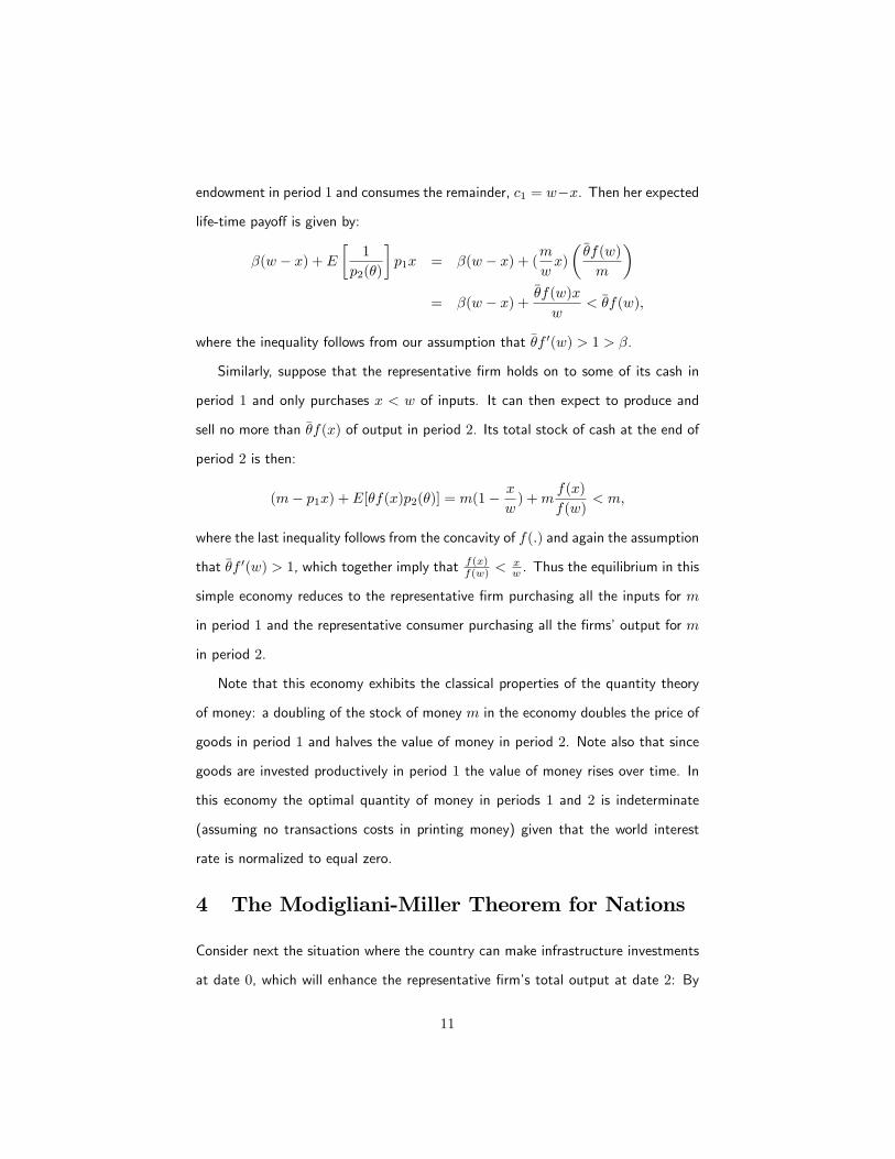
endowment in period 1 and consumes the remainder, c1 = w−x. Then her expected

life-time payoff is given by:

β(w − x) + E

[1

p2(θ)

]p1x = β(w − x) + (

m

wx)

(θf(w)

m

)= β(w − x) +

θf(w)x

w< θf(w),

where the inequality follows from our assumption that θf ′(w) > 1 > β.

Similarly, suppose that the representative firm holds on to some of its cash in

period 1 and only purchases x < w of inputs. It can then expect to produce and

sell no more than θf(x) of output in period 2. Its total stock of cash at the end of

period 2 is then:

(m− p1x) + E[θf(x)p2(θ)] = m(1− x

w) +m

f(x)

f(w)< m,

where the last inequality follows from the concavity of f(.) and again the assumption

that θf ′(w) > 1, which together imply that f(x)f(w) <

xw . Thus the equilibrium in this

simple economy reduces to the representative firm purchasing all the inputs for m

in period 1 and the representative consumer purchasing all the firms’output for m

in period 2.

Note that this economy exhibits the classical properties of the quantity theory

of money: a doubling of the stock of money m in the economy doubles the price of

goods in period 1 and halves the value of money in period 2. Note also that since

goods are invested productively in period 1 the value of money rises over time. In

this economy the optimal quantity of money in periods 1 and 2 is indeterminate

(assuming no transactions costs in printing money) given that the world interest

rate is normalized to equal zero.

4 The Modigliani-Miller Theorem for Nations

Consider next the situation where the country can make infrastructure investments

at date 0, which will enhance the representative firm’s total output at date 2: By

11

spending k > 0 on infrastructure, output is increased by a factor Q(k), where

we assume that Q(0) = 1, Q′ > 0 and Q′′ < 0. The country can raise k from

international capital markets at a world price of 1 (since the world equilibrium

interest rate is normalized to zero). It can pay for this capital by either printing

money (∆− 1)m in period 0 or by promising to repay k out of period 1 output (we

assume for now that the country can commit not to default and not to print more

money after the increment in the money base of (∆− 1)m).

4.1 Increase in the money base

Suppose now that the country raises k from risk-neutral foreign investors against a

payment in domestic currency of (∆− 1)m. The increase (∆− 1)m must then be

at least equal to E[p2(θ)]k. In other words, the foreign sellers of capital in period

0 must be able to purchase a fraction of period 1 output that is expected to equal

to k.

By investing k in infrastructure, the country’s expected period 2 output is then

given by Q(k)θf(w), and for any realization θ the period 1 price of wheat is given

by:

p2(θ) =m∆

θQ(k)f(w).

To make the problem interesting, we assume that the infrastructure investment is

a positive net present value investment:

(Q(k)− 1)θf(w) > k.

To simplify notation let Q(k)f(w) = Ω(k,w). The representative consumer’s prob-

12

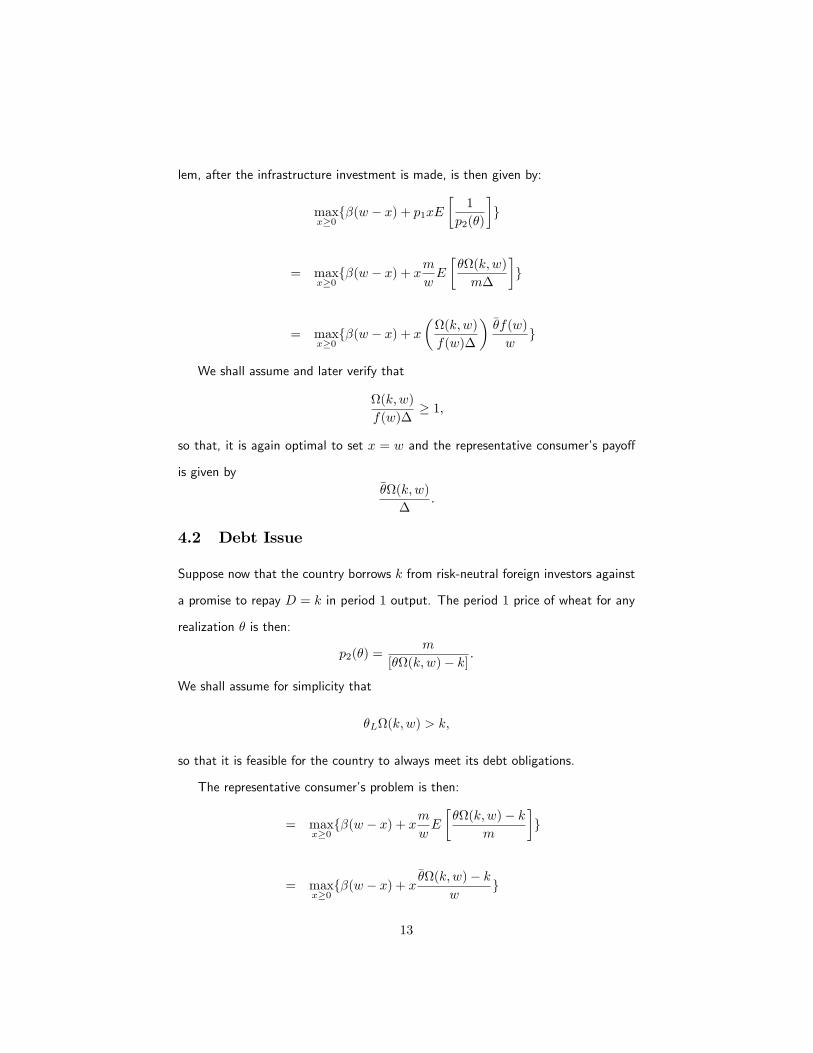
lem, after the infrastructure investment is made, is then given by:

maxx≥0β(w − x) + p1xE

[1

p2(θ)

]

= maxx≥0β(w − x) + x

m

wE

[θΩ(k,w)

m∆

]

= maxx≥0β(w − x) + x

(Ω(k,w)

f(w)∆

)θf(w)

w

We shall assume and later verify that

Ω(k,w)

f(w)∆≥ 1,

so that, it is again optimal to set x = w and the representative consumer’s payoff

is given byθΩ(k,w)

∆.

4.2 Debt Issue

Suppose now that the country borrows k from risk-neutral foreign investors against

a promise to repay D = k in period 1 output. The period 1 price of wheat for any

realization θ is then:

p2(θ) =m

[θΩ(k,w)− k].

We shall assume for simplicity that

θLΩ(k,w) > k,

so that it is feasible for the country to always meet its debt obligations.

The representative consumer’s problem is then:

= maxx≥0β(w − x) + x

m

wE

[θΩ(k,w)− k

m

]

= maxx≥0β(w − x) + x

θΩ(k,w)− kw

13

Recall that Ω(k,w) = Q(k)f(w), and since Q(k) > 1 it is a fortiori optimal to

set x = w, so that the representative consumer’s payoff is:

θΩ(k,w)− k.

4.3 Equivalence

Under Modigliani-Miller equivalence we should have:

θΩ(k,w)

∆= θΩ(k,w)− k,

or,

∆ =θΩ(k,w)

θΩ(k,w)− k.

Now, (∆− 1)m is set so that:

(∆− 1)m

E[p2(θ)]= k,

or

(∆− 1) =k

mE[p2(θ)].

Substituting for

E[p2(θ)] =m∆

θΩ(k,w),

we then obtain:

∆− 1 =k∆

θΩ(k,w),

or

∆ =θΩ(k,w)

θΩ(k,w)− k.

Thus, as expected, when there are no frictions in capital markets it is equivalent

to finance the capital raised from world markets with a domestic money issue (∆−

1)m or with a foreign-currency denominated debt issue with a fixed promised real

repayment of D = k. Actually, the currency denomination of the debt is irrelevant.

Furthermore, the Modigliani-Miller irrelevance result extends to the case of risky

debt with no deadweight costs of default, and to any combination of debt and

money financing.

14

5 Willingness to Inflate and Willingness to Re-pay

In this section we enrich the model by introducing two frictions in international

capital markets that limit sovereign nations’ability to raise funds from investors. A

first friction that is commonly mentioned in the international finance literature is a

country’s willingness to repay its debts problem that raises a country’s cost of issuing

debt claims to foreign investors. A sovereign borrower cannot commit to honor its

debts. It will only choose to repay what it promised to pay if it is in its interest to

repay. As Eaton and Gersovitz (1981) and Bulow and Rogoff (1989) emphasize, a

sovereign will repay only if the cost of default is higher than the servicing cost of

the debt. The willingness-to-repay problem reduces a country’s ability or willingness

to raise funds via debt.

The second friction we introduce is what we refer to as a country’s willingness

to inflate problem. This friction has not been modeled in the international finance

literature and is similar to the equity dilution cost in Myers and Majluf (1984). Just

as a country cannot commit to honor its debts it cannot pledge to limit inflation.

Investors may therefore be concerned about the risk of debasement of the currency

and require compensation for holding claims denominated in the domestic currency

(Jeanne, 2003, invokes the lack of monetary credibility as a key reason why private

sector lending in emerging markets is in the form of foreign-currency debt). If

investors’ perceived risk of debasement is excessive then the nation may incur a

dilution cost of issuing more fiat money. That is, by issuing money to foreign

investors at an excessively low price the nation dilutes the value of the money

balances of domestic residents. In its choice of mode of financing the nation then

trades off the costs of debt stemming from the willingness to repay problem against

the costs of dilution caused by an exaggerated perceived risk of money debasement.

15

5.1 Equity Financing and the Willingness to Inflate Prob-lem

Consider first the situation where the country funds k by printing money (or issuing

domestic currency debt). What are the costs of printing more money? In the spirit

of Myers and Majluf (1984), suppose that a country may be more or less inflation

prone. In period 0 it is not known for sure whether the future government in the

country in period 2 will be a monetary-dove or a monetary-hawk. A monetary-

dove government will expand the money supply in period 2 by (∆1 − 1)∆0m to

fund, say, an increase in pay or pensions of civil servants. This future expansion

in the money base is a pure transfer to domestic residents that results in a higher

nominal price level. In contrast, a monetary-hawk government will not expand the

money supply in period 2 at all, so that ∆1 = 1. Suppose that domestic residents

expect to have a monetary-dove government in period 2 with probability λ ∈ (0, 1).

International investors’beliefs about the propensity of future governments to inflate

do not generally coincide with those of domestic residents.

We denote by µ(∆0) ∈ (0, 1) the conditional probability that international in-

vestors assign to a monetary-dove government in period 1. When the nation in-

creases its money supply (∆0 > 1) at date 0 international investors are likely to put

more weight on the possibility that they may face a monetary-dove government.

We therefore assume that µ′ ≥ 0. However, we do not assume that international

investors (or domestic residents) form rational expectations about the type of gov-

ernment they are likely to face. International investors’beliefs are formed on an

incomplete understanding of the country’s history. They may exhibit extrapolative

bias, and may not fully take account of recent political and social changes in the

country that might alter the likelihood of a future monetary-dove government of

emerging. In particular, international investors’conditional beliefs µ(∆0) may be in-

completely revised in response to the financing choices of the country’s government

16

in period 0. For much of our analysis we shall restrict attention to the situation

where µ(0) = µ < λ and µ(∆0) > λ for a suffi ciently large ∆0.

Consider first the extreme but simpler situation where µ′ = 0. That is, in-

ternational investors do not revise their beliefs at all in response to the country’s

financing choices. If the country funds infrastructure expenditures k by issuing

money (∆0 − 1)m in period 0, the price level for any realization of θ in period 2

will then be

p2(θ) =m∆0∆1

θΩ(k,w)

under a monetary-dove government, and

p2(θ) =m∆0

θΩ(k,w)

under a monetary-hawk government.2

Accordingly, foreign investors will demand a payment in money (∆0 − 1)m in

exchange for the investment k such that:

[µ

E[p2(θ)]+

1− µE[p2(θ)]

](∆0 − 1)m = k

where,

E[p2(θ)] =m∆0∆1

θΩ(k,w)

and

E[p2(θ)] =m∆0

θΩ(k,w).

Substituting for p2(θ) and p2(θ) and rearranging we obtain that:

θΩ(k,w)[µ+ (1− µ)∆1

m∆0∆1](∆0 − 1)m = k

So that:

∆0 =(µ+(1−µ)∆1

∆1)θΩ(k,w)

(µ+(1−µ)∆1

∆1)θΩ(k,w)− k

. (2)

2Note that we assume implicitly here that domestic consumers sell all their endowment tofirms in period 1 so that x = w. It is optimal for domestic consumers to do so if β is lowenough, which we shall assume in the remainder of the analysis.

17

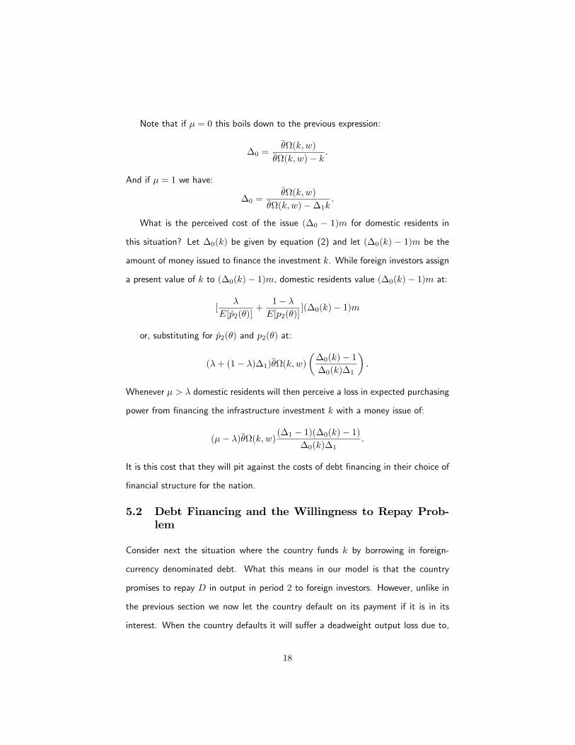
Note that if µ = 0 this boils down to the previous expression:

∆0 =θΩ(k,w)

θΩ(k,w)− k.

And if µ = 1 we have:

∆0 =θΩ(k,w)

θΩ(k,w)−∆1k.

What is the perceived cost of the issue (∆0 − 1)m for domestic residents in

this situation? Let ∆0(k) be given by equation (2) and let (∆0(k) − 1)m be the

amount of money issued to finance the investment k. While foreign investors assign

a present value of k to (∆0(k)− 1)m, domestic residents value (∆0(k)− 1)m at:

[λ

E[p2(θ)]+

1− λE[p2(θ)]

](∆0(k)− 1)m

or, substituting for p2(θ) and p2(θ) at:

(λ+ (1− λ)∆1)θΩ(k,w)

(∆0(k)− 1

∆0(k)∆1

).

Whenever µ > λ domestic residents will then perceive a loss in expected purchasing

power from financing the infrastructure investment k with a money issue of:

(µ− λ)θΩ(k,w)(∆1 − 1)(∆0(k)− 1)

∆0(k)∆1.

It is this cost that they will pit against the costs of debt financing in their choice of

financial structure for the nation.

5.2 Debt Financing and the Willingness to Repay Prob-lem

Consider next the situation where the country funds k by borrowing in foreign-

currency denominated debt. What this means in our model is that the country

promises to repay D in output in period 2 to foreign investors. However, unlike in

the previous section we now let the country default on its payment if it is in its

interest. When the country defaults it will suffer a deadweight output loss due to,

18

say, (unmodeled) trade sanctions and other economic disruptions. Suppose that this

cost is a percentage loss in final output φ > 0, so that after default the country can

only produce and consume (1− φ)θΩ(k,w). Given such a default-cost the country

will choose to default on its debt obligation D if and only if

θΩ(k,w)−D < (1− φ)θΩ(k,w)

or

D > φθΩ(k,w).

Note that the country’s default decision is independent of its monetary policy.

Whether the country is run by a monetary-dove or monetary-hawk government

is irrelevant to the default decision, since under either government the representa-

tive resident obtains the same real output. An expansion in the money supply of

(∆1 − 1)m in this situation involves no dilution costs, as there is no redistribution

of wealth from domestic residents to foreign investors as a result of the mone-

tary expansion. Such an increase in money supply is equivalent to a rights issue,

maintaining the per-capita output share each resident can buy.

Let θD ∈ [θL, θH ] denote the cutoff

θD =D

φΩ(k,w)

at which the country defaults, and led D be the promised debt repayment such that

the country is just able to raise k to fund its investment:

Pr(θ ≥ θD)D = k.

The expected deadweight cost of foreign-currency denominated debt financing is

then given by:

Pr(θ < θD)E[θ | θ < θD]φΩ(k,w).

In other words, while the country is able to fund itself at perceived fair terms by

issuing debt, this may involve a risk of default with the associated deadweight

19

costs of a debt default, which are borne by the country. To the extent that debt

financing of investment requires issuing risky debt, the country may prefer to fund its

investment by issuing fiat money (or domestic-currency debt that can be monetized),

even if it thereby incurs an excessive dilution of ownership (or debasement of the

currency).

5.3 Optimal Financing

How much money and foreign-currency debt should the country issue to interna-

tional investors? We assume that the country’s objective is to maximize the expected

lifetime utility of domestic residents.3 The claims issued to foreign investors serve

not only to fund the investment expenditure k, but also to build foreign-currency

reserves that help the country smooth its terms of trade shocks. To keep the analy-

sis tractable we shall first consider the special case where the country only seeks to

raise suffi cient funds to be able to undertake the investment k. In a second step we

also allow the country to build reserves by issuing claims to international investors.

Furthermore, we shall break down the analysis into a first question of the choice

between 100% debt financing versus 100% equity financing, and a second question

of the optimal ratio of debt and equity financing. For tractability and without much

loss of generality we shall suppose that θ can take only two values, θ ∈ θL, θH

and that Pr(θ = θH) = π ∈ (0, 1).4

Debt Financing. When θ only takes the two values θL and θH , there are

essentially only two possibilities where the country relies on foreign-currency debt

3Note that we do not include the value of the firm V (m2) in the objective function of thecountry. But, to the extent that this value represents the present discounted expected utilityof consumption of (domestic) entrepreneurs, this value will be unaffected by the country’soptimal financing choices, holding infrastructure investment fixed.

4As in Bolton and Jeanne (2007), we can carry out the analysis and obtain closed-formsolutions under the assumption that θ is uniformly distributed on the interval [θL, θH ]. Thealgebra is then more involved and less transparent, as the expected default cost is then givenby the following expression:(

θH −(θ2H − 4k

φΩ(k,w)

) 12

)θHφΩ(k,w)

4− k

2−θ2LφΩ(k,w)

2.

20

financing. Either the country is able to limit its indebtedness so as to always be

willing to service its debt obligations, or the country issues so much debt that in

the unlucky event where the low productivity shock θL is realized it defaults on its

external debt obligations. In the former situation, the maximum debt promise the

country can credibly make is given by D = θLφΩ(k,w), so that a necessary and

suffi cient condition for the country to be able to fund itself with safe debt is:

θLφΩ(k,w) ≥ k. (3)

Suppose that this condition is violated, then the debt promise the country must

make to be able to raise k through an external debt issue is given by D = k/π, and

a necessary condition for risky debt financing is

θHφΩ(k,w) ≥ k

π. (4)

In sum, when condition (4) holds but condition (3) is violated, the country can fund

itself with risky debt and incurs an expected deadweight cost of default given by:

(1− π)θLφΩ(k,w).

Equity Financing. Equity financing when θ only takes the two values θL and

θH involves the following expected dilution cost:

(µ− λ)(πθH + (1− π)θL)Ω(k,w)(∆1 − 1)(∆0(k)− 1)

∆0(k)∆1.

Comparing expected default costs to expected dilution costs, we then obtain the

following condition for the optimality of equity financing:

(µ− λ)(πθH + (1− π)θL)(∆1 − 1)(∆0(k)− 1)

∆0(k)∆1< (1− π)θLφΩ(k,w). (5)

Some simple observations follow from this condition. First, countries that have an

undeserved reputation for being monetary-doves, for which both (µ−λ) and ∆1 are

large, are likely to be better off financing investments through foreign-currency de-

nominated debt. Second, countries that are likely to face large deadweight costs of

21

default φ, perhaps because they are highly financially and economically integrated

in the world economy, may be better off financing their investments by printing

money or issuing domestic-currency claims. Third, the lower is the productivity θL

in a crisis, the less the country has to lose from a default and the more attractive is

funding through external debt. Note that in this latter situation risky debt is attrac-

tive for the issuing country as it enables the country to obtain some consumption

smoothing by, in effect, issuing a state contingent claim at relatively low cost. Risky

debt in this scenario implements similar allocations as GDP-indexed debt.

The optimal debt-equity ratio: Consider next the optimal choice of a com-

bination of debt and equity financing. When condition (3) holds and µ > λ it is

obviously best for the country to fund itself entirely with safe debt. Equally obvi-

ous is the observation that when µ < λ it is strictly preferable for the country to

fund itself entirely through ‘equity’(i.e. money) issuance. In fact, the country may

in this case want to issue even more ‘equity’than it needs to fund its investment

outlays, and build foreign exchange reserves. We will return to a discussion of for-

eign exchange reserves in the next subsection. For now, we will focus on the most

interesting case where µ > λ and condition (4) holds but condition (3) is violated.

In this case the optimal amount of debt financing for the country is either safe

debt combined with equity financing or risky debt and no equity financing. If it is

optimal to issue safe debt combined with equity, then the country’s funding structure

is given by an amount of debt

DL = θLφΩ(k,w),

and an amount of equity (∆0(k −DL)− 1)m, where

∆0(k −DL) =(µ+(1−µ)∆1

∆1)θΩ(k,w)

(µ+(1−µ)∆1

∆1)θΩ(k,w) + θLφΩ(k,w)− k

. (6)

The interest coverage ratio (total debt repayments over GDP) for the country

is then φ in the crisis state, when productivity is low, and θLφθH

in the good state,

22

when productivity is high. When it is optimal to issue only risky debt DH = k/π

and no equity, the interest coverage ratio in the good state is kπθHΩ(k,w) .

5

5.4 Optimal reserves

Consider next the general framework where international investors revise their beliefs

in response to changes in the country’s monetary base, and where µ′ > 0. That is,

an increase in the monetary base of d∆0 induces international investors to increase

their revised beliefs by µ′ that the country will have a monetary-dove government

in period 1. This general framework allows for a richer financial policy than we have

considered so far. In particular, a market timing motive for issuing equity arises in

this framework that is similar to the timing of equity issuance in the ‘market-driven’

corporate finance literature (Baker, 2009).

To see this, note first that if it is the case that µ(0) = µ < λ, so that interna-

tional investors are a priori more confident than domestic residents about the risk

of inflation, then it is weakly optimal for the country to issue at least an amount

∆R in domestic currency under any circumstances, where ∆R is given by

µ(∆R) = λ.

Consider for simplicity the following affi ne function specification for µ(∆R):

µ(∆R) = µ+ γ∆R,

so that the minimum domestic currency issuance to build reserves is

∆R =λ− µγ

. (8)

5Another interesting case is when µ > λ and neither condition (4) nor (3) holds. In thiscase, the country may choose to issue an amount of risky debt

DH = θHφΩ(k,w),

combined with an amount of equity (∆0(k −DH)− 1)m with

∆0(k −DH) =(µ+(1−µ)∆1

∆1)θΩ(k,w)

(µ+(1−µ)∆1

∆1)θΩ(k,w) + θHφΩ(k,w)− k

. (7)

23

By issuing an amount ∆R of domestic currency, the country is then able to build

at no cost a minimum stock of foreign-currency reserves R equal to:

R = [λ

E[p2(θ)]+

1− λE[p2(θ)]

](∆R − 1)m

where,

E[p2(θ)] =m∆R∆1

θΩ(k,w)

and

E[p2(θ)] =m∆R

θΩ(k,w).

Substituting for p2(θ) and p2(θ) and rearranging we obtain that:

R = θΩ(k,w)[λ+ (1− λ)∆1

m∆R∆1](∆R − 1)m,

where ∆R is given by equation (8).

These foreign-currency reserves R can, of course, be used to fund investments

when valuable investment opportunities arise. But, more interestingly, they can

also allow the nation to become more creditworthy, enhancing its debt capacity, as

we illustrate below. A critical condition for enhancing a country’s debt capacity

by relying on foreign-currency reserves is that these reserves be placed in escrow

at an offshore custodian bank, as for example Venezuela has done to finance its

Petrolera Zuata oil-field project (see Esty and Millet, 1998). When this is the case

the country stands to lose all reserves placed in escrow in the event of default on

its debts. By placing foreign currency reserves in escrow, the country is then able

to increase its safe debt capacity as follows. Suppose that the country places its

entire foreign currency reserves R in escrow, then it is able to issue an amount of

safe foreign-currency denominated debt

DL = θLφΩ(k,w) +R.

Indeed, the country will refrain from defaulting on any foreign-currency debt oblig-

24

ation D in the event of a bad productivity shock θL as long as:

θLΩ(k,w) +R−D ≥ θL(1− φ)Ω(k,w)

The RHS of this incentive constraint is the output the country’s residents would

be able to consume following a default. Note that default now involves not only a

lower output but also the loss of foreign-currency reserves. By pledging its foreign-

currency reserves a country is thus able to expand its debt capacity and relax its

financial constraints.

6 Financial Constraints and Debt Overhang

Financing costs, whether in the form of deadweight costs of default or inflation costs,

may be so high that it is simply not worth investing in infrastructure. Suppose the

country is already indebted at time t = 0 and has an outstanding stock of foreign-

currency denominated debt of D0, under what conditions is it worthwhile to invest

in k? We shall address this question in the special case where µ′ = 0 and where

µ > λ, so that there is a perceived dilution cost in issuing domestic currency to

fund k. Consider in turn equity and debt financing.

Equity Financing. When the inherited stock of debt D0 is low enough that

the country always prefers to repay any such low debt obligation, then the choice

between no investment and investment is unaffected by the presence of this debt

under equity financing. To see this, observe that the expected payoff under no

investment is:

(πθH + (1− π)θL)Ω(0, w)−D0.

And, under equity financed investment the expected payoff is:

(1− α(µ))(πθH + (1− π)θL)Ω(k,w)−D0,

where

α(µ) = [µ+ (1− µ)∆1

m∆0∆1](∆0 − 1)m =

k

(πθH + (1− π)θL)Ω(k,w).

25

The country thus prefers an equity-financed investment to no investment if and only

if:

(1− α(µ))(πθH + (1− π)θL)Ω(k,w) ≥ (πθH + (1− π)θL)Ω(0, w),

a condition that is independent of D0.

Debt Overhang. As in Myers (1977), if the inherited stock of debt D0 is so

large that the country would default in the low productivity state (in the absence

of any investment) the debt D0 could discourage the country from undertaking an

equity-financed investment. To see this, suppose that

φθHΩ(0, w) > D0 > φθLΩ(0, w)

so that the expected payoff under no investment is:

π(θHΩ(0, w)−D0) + (1− π)θL(1− φ)Ω(0, w).

Suppose, in addition, that:

D0 ≤ φθLΩ(k,w)

so that under an equity-financed investment the country’s expected payoff is as

before:

(1− α(µ))(πθH + (1− π)θL)Ω(k,w)−D0.

Now, whether the country decides to invest depends on the following condition:

(1−α(µ))(πθH+(1−π)θL)Ω(k,w) ≥ (πθH+(1−π)θL)Ω(0, w)+(1−π)(D0−θLφΩ(0, w))

By assumption, D0 > φθLΩ(0, w), so that for some parameter values we may have:

(1− α(µ))[πθHΩ(k,w) + (1− π)θLΩ(k,w)] ≥ (πθH + (1− π)θL)Ω(0, w)

and

(1−α(µ))(πθH+(1−π)θL)Ω(k,w) < (πθH+(1−π)θL)Ω(0, w)+(1−π)(D0−θLφΩ(0, w)).

26

In such situations D0 is so large that it overhangs the country’s effi cient investment

decision.6

Debt Financing. Consider next debt financing. IfD0 is ‘safe’(D0 < φθLΩ(0, w))

the expected payoff under no investment is:

(πθH + (1− π)θL)Ω(0, w)−D0.

If the country adds D1 to its inherited debt to fund the infrastructure investment,

so that (D1 +D0) > φθLΩ(k,w), then its expected payoff becomes:

π(θHΩ(k,w)−D1 −D0) + (1− π)(1− φ)θLΩ(k,w),

where D1 = kπ . The country thus prefers a debt-financed investment to no invest-

ment if and only if:

π(θHΩ(k,w)− kπ−D0)+(1−π)(1−φ)θLΩ(k,w) ≥ (πθH+(1−π)θL)Ω(0, w)−D0

or, rearranging:

(πθH + (1− π)θL)(Ω(k,w)− Ω(0, w))− k ≥ (1− π)(φθLΩ(k,w)−D0)

Given that φθLΩ(k,w) > φθLΩ(0, w) > D0, an amount of safe inherited debt D0

such that

D0 > φθLΩ(k,w)− k

π

can potentially overhang a debt-financed infrastructure investment. In contrast to

equity financing, for which there is no debt overhang problem as long as inherited

debt D0 is ‘safe’, under debt financing any inherited ‘safe’debt that is suffi ciently

high to force the country into risky debt territory when it funds its investment via

additional debt D1 can result in a debt overhang problem. The point is that by

adding new debt D1 to old debt D0 the country incurs an expected deadweight

6Note that the situation where D0 > φθHΩ(0, w) is not interesting. It would mean thatthe country inherits such a large stock of debt that it would default no matter what.

27

cost of default that acts like a tax on investment. More generally, every time the

country is in a situation where an increase in indebtedness raises the risk of default,

it may face a debt overhang problem if it funds its investments via debt.

If, on the other hand, the inherited stock of debt D0 is already ‘risky’(D0 >

φθLΩ(0, w)) the country prefers a debt-financed investment to no investment if and

only if:

π(θHΩ(k,w)−kπ−D0)+(1−π)(1−φ)θLΩ(k,w) ≥ π(θHΩ(0, w)−D0)+(1−π)(1−φ)θLΩ(0, w)

or, rearranging:

(πθH + (1− π)(1− φ)θL)(Ω(k,w)− Ω(0, w)) ≥ k.

In this case there is no debt overhang as the condition above is independent of the

size of D0. In sum, under a debt-financed investment there is no debt overhang if

inherited debt is risky, while under an equity-financed investment there is no debt

overhang if and only if inherited debt is safe.7

When inherited debt is risky, one might expect that a country would go out

of its way to reduce its indebtedness in an effort to avoid any deadweight costs

of default. But, this turns out not to be in domestic residents’best interests, as

the main beneficiaries in any reduction in the risk of default are the holders of the

inherited debt. When inherited debt is risky, it could actually be in the interest of

domestic residents to increase the country’s indebtedness and risk of default in order

to fund valuable investments. Indeed, the main losers from such an increase in the

country’s indebtedness are the holders of the existing debt. Thus, debt overhang

considerations in a sovereign debt context can give rise to debt dynamics where

7This result is not entirely robust. If there is a positive recovery value of debt after defaultthen whether inherited debt D0 overhangs the country’s investment decision is less clear, asall the country’s foreign-currency denominated debt is pari passu. Adding new debt D1 tothe debt stock D0 will then involve diluting the holders of the inherited debt and thus couldresult in a transfer to the country. This transfer is a form of subsidy, which could encouragethe country to invest even if the net present value of the investment is negative.

28

debt begets debt, to use an expression coined by Admati, DeMarzo, Hellwig and

Pfleiderer (2014).

7 Model Predictions and Empirical Observations

How does the optimal combination of reserves, debt and equity financing, vary with

underlying economic conditions? In particular, how does the choice between safe

and risky debt vary with the underlying economy? The strongest predictions of

the model center around the interplay of two key parameters, θL and φ. As can

be seen from inequality (5), expected costs of default on foreign-currency debt are

highest when both θL and φ are large, and countries for which this is the case are

likely to be better off financing their investments with money even if this involves

paying some inflation costs. Which countries are likely to have both high θL and φ?

Clearly, more developed countries have higher productivity and therefore higher θL.

That is, developed countries remain highly productive even in recessions or crisis

times. Moreover, developed countries have more financially integrated economies

and larger banking sectors. A sovereign debt default for an economy with a banking

sector that is both large and highly integrated in the global economy is likely to

result in a major banking crisis, and therefore the deadweight cost of default will

be significantly larger when the banking sector is also affected, thus resulting in a

larger φ.

In contrast, countries for which it is likely to be preferable to rely on risky foreign-

currency debt financing are poor countries that are likely to have low productivity

in a crisis and are less dependent on the banking system to operate. To the extent

that these countries have a lower cost of default they might be better off issuing

risky debt. If they limit themselves to only safe debt issuance DL they would have

to mostly fund their investments through domestic currency debt issuance, which

could come at a high cost of dilution.

29

While our theoretical analysis is mostly normative and does not necessarily reflect

actual financing choices by countries, it is nevertheless instructive to contrast the

major observed differences in countries’ financial structures and foreign currency

reserve management. We begin by describing the capital structures of four countries

that rely on virtually no foreign-currency debt. We compare the experience of these

countries with first Argentina, a country that has heavily relied on foreign-currency

debt and suffered a major debt crisis, and second the Euro Zone, which as a result

of monetary union has, in effect, converted domestic-currency debt into foreign-

currency debt. Finally, we compare the experience of three very different economies

that have in common a policy of accumulating very large foreign-currency reserves.

7.1 Domestic-currency Debt: The U.S., U.K., China andJapan compared

A common belief is that only advanced countries and reserve-currency countries

can afford to rely predominantly on domestic-currency debt. While it is true that

countries whose currency is a reserve asset have an ‘exorbitant privilege’8 that

allows them to issue debt denominated in their currency at favorable terms, reliance

on domestic-currency debt is by no means confined to them, or to countries with

advanced economies.9 As as the comparison between the U.S., U.K., Japan and

China in this section illustrates, from 1993 to 2013 the ratio of foreign-currency

debt to GDP in the U.S., U.K. and Japan has never exceeded respectively, 0.05%,

1.1%, 0.14%, while for China it has not exceeded 0.5% (see Figure 1).

These four countries also look very similar in terms of their ratios of M2+

Domestic-currency Debt-to-GDP ratios, as Figure 2 illustrates. TheM2+ Domestic-

currency Debt measure of the money stock is closest in our view to the m (m∆0

and m∆0∆1) variable in the model. This ratio has increased from 120% in 1993

8See Gourinchas and Rey (2007).9Du and Schreger (2015) study the currency composition of sovereign debt of 13 emerging

market countries and find that over the past decade the share of domestic-currency debt forthese countries has increased from 15 to 60 percent on average.

30

to 180% in 2014 for the U.S., from under 100% in 1993 to nearly 250% in 2014 for

the U.K., from 215% in 1993 to 300% in 2014 for Japan, and from 100% in 1993

to nearly 210% in 2014 for China. Remarkably, despite what appear to be large in-

creases in the money stock to GDP ratio in these countries, there has been subdued

inflation over this twenty-year period in each of these countries, as Figure 3 shows.

Except for the financial crisis of 2008-2009, the inflation rate in the U.S. from 1993

to 2014 has hovered around 2% and never exceeded 4%. The inflation experience

of the U.K. is very similar, with inflation peaking at just under 4.5% in 2011. As

for Japan, its rate of inflation has, if anything, been in deflation territory over this

period, hovering around 0%, with the very recent exception of a peak inflation of

2.7% in 2014. Finally, China’s inflation rate over this period has come down from

a peak of 24% in 1994 to hover around 3% over the remainder of this period, with

another peak at 5.8% in 2008. China was able to bring down its high inflation rate

in 1995 and did contract its M2+ Domestic-currency Debt in 1994 and 1995. This

was a key step to reaffi rm its reputation as a low-inflation emerging-market country,

and thus preserve its ability to finance its high rate of growth and investment with

domestic currency at favorable terms.

The four countries’ experience, however, differs significantly in two respects.

First, and most obviously the rate of GDP growth, which hovered around 3% in

the U.S. and U.K. (with the exception of the financial crisis when it dropped to

respectively −2.8% and −4.3% in the U.S. and U.K. and thereafter averaged around

2%), and around 1.5% for Japan (with a drop in 2009 to −5.5%). In contrast,

China’s GDP growth over this period started at a peak of 14% in 1993, continued at

an average rate of around 10% to reach a trough of 7.3% in 2014 (and, remarkably,

with a growth rate of 9.2% in 2009). Second, China’s foreign-currency reserves

were at 3.3% of GDP in 1993 and ended at just under 40% in 2014. Similarly,

Japan’s foreign currency reserves to GDP ratio shot up from 7.3% in 2000 to 26%

in 2014. Meanwhile, the U.S. foreign currency reserves never exceeded 0.35% over

31

this period and the U.K.’s reserves peaked at just under 1% in 2003.

Part of the rise in foreign currency reserves reflects the fact that China and Japan

ran large current account surpluses (and the U.S. and U.K. large current account

deficits). As Figure 4 highlights, China’s current account over this period was in

surplus, rising from 1.3% of GDP in 1994 to a peak of 10.5% in 2007 and then

declining back to a surplus of 2.1% in 20014. Similarly, Japan’s current account

surplus was 3% of GDP in 1993, peaked at 5.1% in 2007 and subsequently declined

to 0.5% in 2014. In contrast, the current accounts of the U.S. and the U.K. are

almost mirror images of those of China and Japan, with the U.S. running a deficit

during this entire period, starting with −1.7% of GDP in 1994, peaking at −5.8%

in 2006 and declining back to −2.4% in 2014 (the U.K. had a deficit of −0.35%

in 1994, −3.7% in 2008, and −5.5% in 2014). While contributing substantially to

the accumulation of foreign currency reserves (roughly around 2/3), these current

account surpluses alone cannot entirely explain the sharp increase in reserves in

China and Japan.

In sum, China’s experience resembles in many ways the financing patterns of a

growth firm, which keeps its leverage low so as to preserve its financing capacity

to pursue future investment opportunities, and which regularly returns to equity

markets to raise new funds for investment. In contrast, the U.S., U.K. experience

resembles more the financing pattern of a mature, blue-chip, company that pays

out a large dividend and times the equity market to raise new funding on the cheap.

7.2 Foreign-currency Debt: Argentina

If there is one country that perfectly fits the common belief that emerging-market

countries have no choice but to issue foreign-currency debt it is Argentina. The

fear of inflation led Argentina to adopt a currency board, which, in effect, insti-

tutionalized reliance on foreign-currency debt. As can be seen in Figure 5, Panel

A, Argentina had a ratio of foreign-currency debt to GDP of just under 10% in

32

1993. This ratio steadily increased and peaked at 70% in 2002, the year in which

Argentina defaulted on this debt and plunged the country in a severe recession,

with a GDP contraction of −11% (see Panel C). Although Argentina subsequently

reached a debt restructuring agreement with a large majority of its debt holders in

2005, thus lowering its foreign-currency debt to GDP ratio to 23.5%, its continuing

legal battles with hold-out creditors in effect shut out Argentina from international

foreign-currency debt markets, so much so that its foreign-currency-debt-to-GDP

ratio continued to decline to 7.8% in 2014.

Being shut out of international debt markets, inevitably pushed Argentina to

rely more on domestic currency financing, as can be seen in Panel B of Figure 5,

which plots Argentina’s M2+ Domestic-currency Debt-to-GDP ratio. This ratio

was at 20% in 2001 and thereafter jumped to hover around 38%. By defaulting on

its foreign-currency debt, and thereby removing its debt-overhang, Argentina was

able to clock up a relatively high GDP growth performance after 2002, as Panel

C of Figure 5 reveals, but it also suffered a bout of remarkably high inflation in a

global context of low inflation: Panel D of Figure 5 shows that Argentina’s inflation

went from 8% in 2006 to 39% in 2014! In sum, Argentina’s experience is certainly

a narrative of severe financial constraints, but also one of runaway public finances.

There is no easy financial fix for a structural public deficit problem. The outcome

is either default or inflation. It is important to note that the fundamental cause

behind high inflation or hyperinflation is generally not simply an overly permissive

monetary policy, but a structural excess public spending problem aided and abetted

by a lax monetary policy.10

10Neil Irwin in The Alchemists points out that Rudolf Von Havenstein the President of theGerman Reichsbank from 1908 to 1923 viewed hyperinflation as “the fault of the governmentfor running huge budget deficits”, and quotes from a telling speech Havelstein gave on August17, 1923: “The Reichbank today issues 20,000 milliard marks of new money daily. In the nextweek the bank will have increased this to 46,000 milliards daily...The total issue at presentamounts to 63,000 milliards. In a few days we shall therefore be able to issue in one daytwo-thirds of the total circulation.” [Neil Irwin, The Alchemists, 2013, pp 52]

33

7.3 Foreign-currency Debt: The Eurozone Experiment

Another experiment, which amounts to a conversion of domestic-currency debt into

foreign-currency debt a la Argentina is the European monetary union. By sep-

arating fiscal and monetary policy, entrusting the conduct of monetary policy to

an independent supra-national central bank, and by enshrining the impossibility of

debt monetization into the monetary union treaty, the European monetary union,

in effect, converted all existing domestic-currency debt of the member states into

foreign-currency debt, thus exposing the member states to the risk of default. In ad-

dition, monetary union effectively shut down any possibility of funding investments

or building foreign exchange reserves through money issuance. Thus, from a corpo-

rate finance perspective one of the important consequences of European monetary

union has been the imposition of the requirement that all future financing be in the

form of foreign-currency debt. It is as if a corporation put in its bylaws that no new

equity issuance is possible and that all new financing of realized operating losses or

investments be through debt. In light of this restriction it is not entirely surprising

that following the global financial crisis of 2007-09 the Eurozone is the only set of

developed countries that has as a consequence faced a sovereign debt crisis.

Figure 6 shows the dramatic effect of monetary union on the member countries’

foreign-currency debt to GDP ratios. In one stroke Italy’s ratio jumped from 4.5%

in 1998 to 109% in 1999, Spain’s ratio jumped from 4.7% to 61%, Germany’s

from 0% to 60%, Portugal’s from 11% to 51%, and Greece’s from 13% to 102%.

Subsequently, this ratio continued to rise in Portugal and Greece due to the perceived

low cost of borrowing. This cost was, of course, much lower than the previous

interest rates on domestic currency debt, which reflected inflation risk as perceived

by financial markets. Monetary union, substantially reduced, if not eliminated,

this risk (see Figure 6). At the same time, financial markets priced in an implicit

guarantee by the union against the risk of default by periphery countries. Spain’s

34

foreign-currency debt to GDP ratio declined up to the crisis (the debt build-up

took place in the private sector) and Italy’s and Germany’s ratios remained stable.

But the financial crisis of 2007-09 led to a further increase, which was due to

a combination of a decline in the denominator (GDP) and a rise in the cost of

borrowing in the periphery due to a change in financial markets’perception about

the risk of default. Thus, Germany’s ratio rose from 64% in 2007 to 80% in 2010;

Italy’s ratio rose from 100% in 2007 to 132% in 2014; Spain’s ratio jumped from

35.5% in 2007 to 98% in 2014; Portugal’s ratio went from 68% in 2007 to 130%

in 2014, and Greece’s ratio, despite a major debt write-down in the second rescue

package, went from 124% in 2007 to 188% in 2014. The financial crisis made

apparent a major debt-overhang problem for member countries of the Eurozone.

It is thus not surprising that these countries stopped growing after the financial

crisis, as Figure 7 shows. The European Central Bank’s proactive policy after the

financial crisis has helped reassure markets about default risk and has brought down

yields across the Eurozone, but it has not helped in any significant way reduce the

debt-overhang problem created by monetary union and exacerbated by the financial

crisis.

7.4 Foreign-exchange Reserves: Switzerland, China andJapan compared

Another recent example of a country that has rapidly built huge foreign-currency

reserves without paying any inflation cost is Switzerland, which in a period of five

years, from 2007 to 2012, increased its reserves to GDP ratio from under 10% to

over 70%, as can be seen in Panel A of Figure 8. Over the same time period

Switzerland’s M2+ Domestic-currency Debt to GDP ratio jumped from just over

170% to over 220% (see Panel B). Yet, inflation dropped from a rate of 2.5% in

2007 to deflation territory by 2014, as can be seen in Panel C. Finally, although

Switzerland’s GDP-growth rate collapsed from 4% in 2007 to −2% in 2009, as a

35

result of the global financial crisis, thereafter it has largely recovered to pre-crisis

levels, as Panel D illustrates.

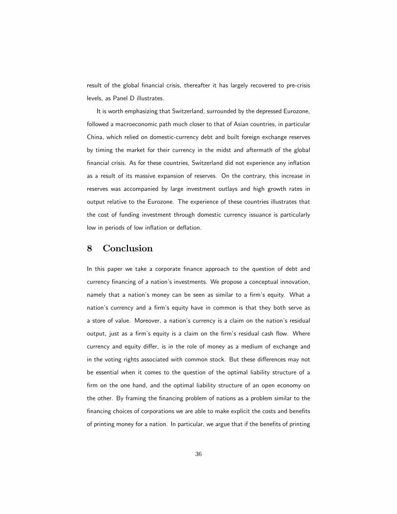
It is worth emphasizing that Switzerland, surrounded by the depressed Eurozone,

followed a macroeconomic path much closer to that of Asian countries, in particular

China, which relied on domestic-currency debt and built foreign exchange reserves

by timing the market for their currency in the midst and aftermath of the global

financial crisis. As for these countries, Switzerland did not experience any inflation

as a result of its massive expansion of reserves. On the contrary, this increase in

reserves was accompanied by large investment outlays and high growth rates in

output relative to the Eurozone. The experience of these countries illustrates that

the cost of funding investment through domestic currency issuance is particularly

low in periods of low inflation or deflation.

8 Conclusion

In this paper we take a corporate finance approach to the question of debt and

currency financing of a nation’s investments. We propose a conceptual innovation,

namely that a nation’s money can be seen as similar to a firm’s equity. What a

nation’s currency and a firm’s equity have in common is that they both serve as

a store of value. Moreover, a nation’s currency is a claim on the nation’s residual

output, just as a firm’s equity is a claim on the firm’s residual cash flow. Where

currency and equity differ, is in the role of money as a medium of exchange and

in the voting rights associated with common stock. But these differences may not

be essential when it comes to the question of the optimal liability structure of a

firm on the one hand, and the optimal liability structure of an open economy on

the other. By framing the financing problem of nations as a problem similar to the

financing choices of corporations we are able to make explicit the costs and benefits

of printing money for a nation. In particular, we argue that if the benefits of printing

36

money in terms of added financing of valuable investments are substantial they may

justify paying the potential costs of inflation.

We have only taken a first step in the formal analysis by specifying an extremely

simple static model. As compelling as the analogy between a firm and a country is,

one important aspect we have oversimplified and which deserves further research is

the fact that a country is not quite a company, as Krugman (1996) has observed.

The non-tradeable sector of a country’s economy is a closed system, which responds

to monetary and fiscal stimulus when depressed. Macroeconomic stimulus involves

other funding considerations, which we have abstracted from entirely.

Another area worth exploring is the dynamics of a nation’s capital structure.

How frequently should a nation rely on money issues? When should it build up

and draw down its foreign currency reserves? And what should be the maturity

of its foreign currency debt? Finally, a fundamental area which requires further

analysis is governance and moral hazard problems in how nations are governed.

We have assumed for simplicity that funding and investment decisions are made by

the government of a nation in the best interest of its citizens. But this is hardly

a realistic description of how most nations are governed. For common stock in

corporations shareholders have voting rights, which they can exercise to appoint

boards of directors and CEOs that pursue policies in their best interest. Corpora-

tions also restrict CEO discretion on equity issuance and buybacks, which require

shareholder approval. Furthermore, corporations are disciplined by corporate law,

which constrains CEOs ability to pursue policies that are detrimental to shareholder

value.

Countries also have institutions that allow citizens to bring to power governments

that act in their interest. But these institutions are very different from corporate

governance and they do not link a citizen’s (or non-citizen’s) voting rights to do-

mestic currency holdings (at least not directly). How does this separation between

control rights and residual rights to the nation’s output affect the question of how

37

nations should be financed? How does it affect the discretion given to governments

to print money? We leave these questions for future research.

References

[1] Admati, A. R., DeMarzo, P. M., Hellwig, M. F., and Pfleiderer, P. C. (2014)

“The Leverage Ratchet Effect”, http://ssrn.com/abstract=2304969

[2] Baker, M. (2009) “Capital Market-Driven Corporate Finance”, Annual Review

of Financial Economics, Vol. 1: 181-205

[3] Bolton, P. and O. Jeanne (2007) “Structuring and Restructuring Sovereign

debt: The Role of a Bankruptcy Regime,”Journal of Political Economy 115(6),

901-924.

[4] Bulow, J. and K. Rogoff. (1989) “A Constant Recontracting Model of Sov-

ereign Debt”, Journal of Political Economy, 97: 155—78.

[5] Burnside, C., Eichenbaum, M. and S. Rebelo (2001) “Prospective deficits and

the Asian currency crisis” Journal of Political Economy 109: 1155—98.

[6] Caballero, R. and Panageas, S. (2007) “A global equilibrium model of sudden

stops and external liquidity management” MIT, Department of Economics,

Discussion Paper

[7] Calvo, G. (1988) “Servicing the public debt: the role of expectations”American

Economic Review 78, 647—661.

[8] Chang, R. and A. Velasco (2000) “Liquidity Crises in Emerging Markets:

Theory and Policy,” in NBER Macroeconomics Annual 1999, ed. by Ben S.

Bernanke and Julio Rotemberg (Cambridge, MA: MIT Press).

[9] Cole, H. and Kehoe, T. (2000) “Self-fulfilling debt crises”Review of Economic

Studies, 67(1): 91—116.

38

[10] Dittmar, A. and A. Thakor (2007) “Why Do Firms Issue Equity?” Journal of

Finance, Vol. 62, No. 1: 1-54

[11] Dooley, M.P., Folkerts-Landau, D. and Garber, P. (2004) “The revived Bretton

Woods system: the effects of periphery intervention and reserve management

on interest rates and exchange rates in center countries”NBER Working Paper

No. 10332.

[12] Du, W. and Schreger, J. (2015) “Sovereign Risk, Currency Risk, and Corporate

Balance Sheets”Harvard, Department of Economics Working Paper

[13] Eaton, J., and Gersovitz, M. (1981) “Debt with Potential Repudiation: Theo-

retical and Empirical Analysis.”Review of Economic Studies, 48(2): 289—309

[14] Eichengreen B., R. Hausmann and U. Panizza (2003), “The pain of original

sin”, in Eichengreen et al., Other People’s Money - Debt Denomination and Fi-

nancial Instability in Emerging Market Economies, University of Chicago Press,

Chicago and London.

[15] Esty, B. C., and Millet, M. M. (1998) “Petrolera Zuata, Petrozuata C.A.”HBS

No. 299-012. Boston: Harvard Business School Publishing

[16] Friedman, M. (1969) “The Optimum Quantity of Money,” in The Optimum

Quantity of Money and Other Essays. Chicago: Aldine Publishing Company.

[17] Gourinchas, P.O., and Rey, H. (2007) “From world banker to world venture cap-

italist: The U.S. external adjustment and the exorbitant privilege” in Richard

Clarida (ed.): G7-Current Account Imbalances: Sustainability and Adjustment,

University of Chicago Press, Chicago

[18] Hahn, F. H. (1965) “On some problems of proving the existence of an equi-

librium in a monetary economy”, in F.H. Hahn and F.P.R. Brechling eds., The

Theory of Interest Rates, London: Macmillan

39

[19] Hahn, F. H. (1982) Money and Inflation, Oxford: Basil Blackwell

[20] Irwin, N. (2013) The Alchemists: Three Central Bankers and A World On Fire,

Penguin Books, New York

[21] Jeanne, O. (2007) “International reserves in emerging market countries: too

much of a good thing?” in (W.C. Brainard and G.L. Perry, eds.), Brookings

Papers on Economic Activity, 1—55, Washington DC: Brookings Institution.

[22] Jeanne, O. (2009) “Why Do Emerging Market Economies Borrow in Foreign

Currency?” IMF Working Paper 03/177

[23] Jeanne, O. (2009) “Debt Maturity and the International Financial Architec-

ture”American Economic Review 99(5): 2135-48

[24] Jeanne, O. and Zettelmeyer, J. (2005) “Original Sin, Balance-Sheet Crises, and

the Roles of International Lending.”In Other People’s Money: Debt Denomina-

tion and Financial Instability in Emerging Market Economies, Eichengreen, B.

and Hausmann, R. (eds) 95—121. Chicago and London: University of Chicago

Press

[25] Krugman, P. (1988) “Financing vs. Forgiving a Debt Overhang” Journal of

Development Economics 29: 253-68

[26] Krugman, P. (1996) “A Country is not a Company”, Harvard Business Review,

January-February Issue

[27] Malmendier, U. and S. Nagel (2014) “Learning from Inflation Experiences”

Quarterly Journal of Economics (forthcoming)

[28] Myers, S.C. (1977) “The Determinants of Corporate Borrowing”, Journal of

Financial Economics, 5: 147-175

40

[29] Myers, S.C. (1984) “The Capital Structure Puzzle”, Journal of Finance Vol.

XXXIX, pp. 575-592.

[30] Myers, S.C. and N.S. Majluf (1984) “Corporate Financing and Investment

Decisions when Firms have Information that Investors do not have”, Journal

of Financial Economics 13, pp. 187-221.

[31] Sachs, J. (1984) “Theoretical Issues in International Borrowing” Princeton

Studies in International Finance 54.

[32] Scheinkman, J. and W. Xiong (2003) “Overconfidence and Speculative Bub-

bles”, Journal of Political Economy 111 (6), 1183-1220

41

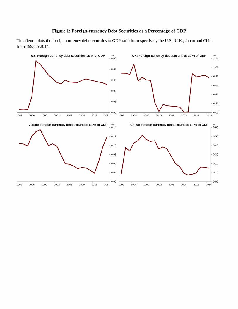
Figure 1: Foreign-currency Debt Securities as a Percentage of GDP

This figure plots the foreign-currency debt securities to GDP ratio for respectively the U.S., U.K., Japan and China from 1993 to 2014.

0.00

0.01

0.02

0.03

0.04

0.05

1993 1996 1999 2002 2005 2008 2011 2014

%US: Foreign-currency debt securities as % of GDP

0.00

0.20

0.40

0.60

0.80

1.00

1.20

1993 1996 1999 2002 2005 2008 2011 2014

%UK: Foreign-currency debt securities as % of GDP

0.02

0.04

0.06

0.08

0.10

0.12

0.14

1993 1996 1999 2002 2005 2008 2011 2014

%Japan: Foreign-currency debt securities as % of GDP

0.00

0.10

0.20

0.30

0.40

0.50

0.60

1993 1996 1999 2002 2005 2008 2011 2014

%China: Foreign-currency debt securities as % of GDP

Figure 2: M2+ Domestic-currency Debt as a Percentage of GDP

This figure plots the sum of M2 and Domestic-currency Debt as a percentage of GDP for respectively the U.S., U.K., Japan and China from 1993 to 2014.

100

110

120

130

140

150

160

170

180

1993 1996 1999 2002 2005 2008 2011 2014

%US: M2 + Domestic currency debt as % of GDP

70

90

110

130

150

170

190

210

230

250

1993 1996 1999 2002 2005 2008 2011 2014

%UK: M2 + Domestic currency debt as % of GDP

210

220

230

240

250

260

270

280

290

300

1993 1996 1999 2002 2005 2008 2011 2014

%Japan: M2 + Domestic currency debt as % of GDP

90

110

130

150

170

190

210

1993 1996 1999 2002 2005 2008 2011 2014

%China: M2 + Domestic currency debt as % of GDP

Figure 3: Inflation

This figure plots the inflation rate for respectively the U.S., U.K., Japan and China from 1993 to 2014.

-0.5

0.0

0.5

1.0

1.5

2.0

2.5

3.0

3.5

4.0

1993 1996 1999 2002 2005 2008 2011 2014

%US: Inflation rate

0.5

1.0

1.5

2.0

2.5

3.0

3.5

4.0

4.5

1993 1996 1999 2002 2005 2008 2011 2014

%UK: Inflation rate

-1.5

-1.0

-0.5

0.0

0.5

1.0

1.5

2.0

2.5

3.0

1993 1996 1999 2002 2005 2008 2011 2014

%Japan: Inflation rate

-5

0

5

10

15

20

25

1993 1996 1999 2002 2005 2008 2011 2014

%China: Inflation rate

Figure 4: GDP Growth

This figure plots the GDP growth rate for respectively the U.S., U.K., Japan and China from 1993 to 2014.

-3

-2

-1

0

1

2

3

4

5

1993 1996 1999 2002 2005 2008 2011 2014

%US: GDP growth rate

-5

-4

-3

-2

-1

0

1

2

3

4

5

1993 1996 1999 2002 2005 2008 2011 2014

%UK: GDP growth rate

-6

-4

-2

0

2

4

6

1993 1996 1999 2002 2005 2008 2011 2014

%Japan: GDP growth rate

0

2

4

6

8

10

12

14

16

1993 1996 1999 2002 2005 2008 2011 2014

%China: GDP growth rate

Figure 5: Argentina

This figure plots the Foreign exchange reserve as a percentage of GDP, sum of M2 and Domestic-currency Debt as a percentage of GDP, inflation rate, and GDP growth rate for Argentina from 1993 to 2014.

2

4

6

8

10

12

14

1993 1996 1999 2002 2005 2008 2011 2014

%Argentina: Foreign exchange reserve as % of GDP

5

10

15

20

25

30

35

40

45

50

1993 1996 1999 2002 2005 2008 2011 2014

%Argentina: M2 + Domestic currency debt as % of GDP

-5

0

5

10

15

20

25

30

35

40

1993 1996 1999 2002 2005 2008 2011 2014

%Argentina: Inflation rate

-15

-10

-5

0

5

10

1993 1996 1999 2002 2005 2008 2011 2014

%Argentina: GDP growth rate

Figure 6: Foreign-currency Debt Securities as a Percentage of GDP

This figure plots the foreign-currency debt securities to GDP ratio for respectively Italy, Spain, Portugal, Germany and Greece from 1993 to 2014.

0

20

40

60

80

100

120

140

1993 1996 1999 2002 2005 2008 2011 2014

%Italy: Foreign-currency debt securities as % of GDP

0

10

20

30

40

50

60

70

80

90

100

1993 1996 1999 2002 2005 2008 2011 2014

%Spain: Foreign-currency debt securities as % of GDP

0

20

40

60

80

100

120

140

1993 1996 1999 2002 2005 2008 2011 2014

%Portugal: Foreign-currency debt securities as % of GDP

0

10

20

30

40

50

60

70

80

90

1993 1996 1999 2002 2005 2008 2011 2014

%Germany: Foreign-currency debt securities as % of GDP

0

20

40

60

80

100

120

140

160

180

200

1993 1996 1999 2002 2005 2008 2011 2014

%Greece: Foreign-currency debt securities as % of GDP

Figure 7: GDP Growth

This figure plots the GDP growth rate for respectively Italy, Spain, Portugal, Germany and Greece from 1993 to 2014.

-6

-5

-4

-3

-2

-1

0

1

2

3

4

1993 1996 1999 2002 2005 2008 2011 2014

%Italy: GDP growth rate

-4

-3

-2

-1

0

1

2

3

4

5

6

1993 1996 1999 2002 2005 2008 2011 2014

%Spain: GDP growth rate

-5

-4

-3

-2

-1

0

1

2

3

4

5

1993 1996 1999 2002 2005 2008 2011 2014

%Portugal: GDP growth rate

-6

-4

-2

0

2

4

6

1993 1996 1999 2002 2005 2008 2011 2014

%Germany: GDP growth rate

-10

-8

-6

-4

-2

0

2

4

6

8

1993 1996 1999 2002 2005 2008 2011 2014

%Greece: GDP growth rate

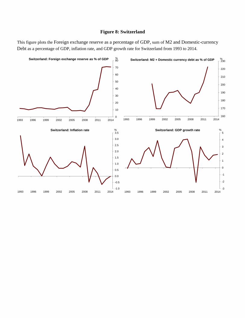
Figure 8: Switzerland

This figure plots the Foreign exchange reserve as a percentage of GDP, sum of M2 and Domestic-currency Debt as a percentage of GDP, inflation rate, and GDP growth rate for Switzerland from 1993 to 2014.

0

10

20

30

40

50

60

70

80

1993 1996 1999 2002 2005 2008 2011 2014

%Switzerland: Foreign exchange reserve as % of GDP

160

170

180

190

200

210

220

230

1993 1996 1999 2002 2005 2008 2011 2014

%Switzerland: M2 + Domestic currency debt as % of GDP

-1.0

-0.5

0.0

0.5

1.0

1.5

2.0

2.5

3.0

3.5

1993 1996 1999 2002 2005 2008 2011 2014

%Switzerland: Inflation rate

-3

-2

-1

0

1

2

3

4

5

1993 1996 1999 2002 2005 2008 2011 2014

%Switzerland: GDP growth rate