'1

i

The Calibration of Balances

David B. Prowse

�=-... im:��·S---1, UBF�ARY !

CSIRO .

'i b<c,I. � \ fr

� DJ\R\:\llN � ! tE·,oni;TORIESJi_,,.._�;.:;....o:=.:.:...:...,�=�

Commonwealth Scientific and Industrial

Research Organization, Australia

1985

National Library of Australia Cataloguing-in-Publication En!ry

Prowse, David B., 1938-The calibration of balances.

Bibliography. Includes index. ISBN O 643 03829 9.

1. Balance - Calibration. I. Commonwealth Scientificand Industrial Research Organization,Australia. II. Title.

681' .2

© CSIRO Australia 1985. Printed by CSIRO, Melbourne

85.192-3040

CONTENTS

Page 1 INTRODUCTION . . .. . .. . .. . .. . .. . . . .. . . . . . .. . .. .. . . .. .. .. . . .. . . . .. . .. . . .. . . .. .. .. .. . .. . .. .. . .. 1

1.1 Introduction and Outline.............................................................. 1 1.2 A Note on the Interpretation of Measurements on Balances ............. 2

2 DEFINITIONS AND SYMBOLS ........................................................ . 2.1 Definitions ................................................................................ . 2.2 Symbols .................................................................................... .

3 TYPES OF BALANCES ..................................................................... .

3.1 Two-Pan, Three-Knife-Edge Balances ......................................... .. 3 .1.1 Damped balances ............................................................... . 3 .1.2 U ndamped or free-swinging balances .................................. ..

3.2 Single-Pan, Two-Knife-Edge Balances ......................................... .. 3.3 Electromagnetic-Force-Compensation Balances ............................. .

2

2 4

5 5 6 6

6

7

4 CALIBRATION OF TWO-PAN, THREE-KNIFE-EDGE BALANCES... 8 4.1 Repeatability of Reading.............................................................. 8 4.2 Sensitivity................................................................................... 9 4.3 Parallelism of Knife Edges............................................................ 10 4.4 Ratio of Arms . . .. . .. . .. .. . . . . .. .. . .. . . . .. .. .. . .. .. . . . . . .. . .. . . . . . .. .. ... . .. . .. . .. .. . .. . .. .. 11 4.5 Uniformity of Scale ..................................................................... 12 4.6 Rider Bar.................................................................................... 12 4. 7 Effect of Off-Centre Loading .... ...... ....... ... .. .. .... .. .... ..... .... ............ 12 4.8 Masses Associated with the Balance............................................... 13 4.9 The Balance Arrestment ............................................................... 13 4.10 User Tests on Balances.................................................................. 14 4.11 Recording and Reporting of Results for Two-Pan Balances.............. 14

4.11.1 Repeatability of reading..................................................... 15 4.11.2 Sensitivity......................................................................... 17 4.11.3 Parallelism of knife edges................................................... 18 4.11.4Ratio of arms .................................................................... 19 4.11.5 Uniformity of scale............................................................ 20 4.11.6 Rider bar.......................................................................... 22 4.11. 7 Effect of off-centre loading . . ...... . .. .. . .. .. .. . ... .. .. . . ... . . ..... ... .. .. . 22 4.11.8 Calibration of masses associated with the balance .. . . .. ... ... .. ... 22 4.11.9 Sample report on a three-knife-edge balance......................... 23

5 CALIBRATION OF SINGLE-PAN, TWO-KNIFE-EDGE BALANCES.. 25 5 .1 Repeatability of Reading.............................................................. 25 5.2 Scale Value.................................................................................. 26 5. 3 Uniformity of Scale .. .. .. .. .. . .. .. .. . .. .. .. . .. .. . .. .. . .. .. .. . .. .. .. . .. .. .. . .. .. . .. .. .. .. 26

5.3.1 A set of calibrated masses is available.................................... 26 5.3.2 A set of calibrated masses is not available .............................. 27 5.3.3 Interpolating between scale divisions..................................... 28

5 .4 Effect of Off-Centre Loading .. .. .. . .. .. .. . .. .. .. .. . .. . .. .. .. .. .. .. .. .. .. .. .. .. .. .. . 28

National Library of Australia Cataloguing-in-Publication Entry

Prowse, David B., 1938-The calibration of balances.

Bibliography. Includes index. ISBN O 643 03829 9.

1. Balance - Calibration. I. Commonwealth Scientificand Industrial Research Organization,Australia. II. Title.

681'.2

© CSIRO Australia 1985. Printed by CSIRO, Melbourne

85.192-3040

CONTENTS

Page 1 INTRODUCTION . .. . . . . .. .. . .. . . .. .. . . . .. .. .. .. .. . .. .. .. . . .. . . .. .. .. . . .. .. .. . .. .. . . .. .. . .. . .. . 1

1.1 Introduction and Outline.............................................................. 1 1.2 A Note on the Interpretation of Measurements on Balances ............. 2

2 DEFINITIONS AND SYMBOLS ....................................................... ..

2.1 Definitions ................................................................................ .

2.2 Symbols ................................................................................... ..

3 TYPES OF BALANCES .................................................................... ..

3.1 Two-Pan, Three-Knife-Edge Balances ......................................... ..

3.1.1 Damped balances .............................................................. ..

3.1.2 Undamped or free-swinging balances ................................... .

3.2 Single-Pan, Two-Knife-Edge Balances ......................................... .. 3. 3 Electromagnetic-Force-Compensation Balances ............................ ..

2

2 4

5 5

6 6 6 7

4 CALIBRATION OF TWO-PAN, THREE-KNIFE-EDGE BALANCES... 8 4.1 Repeatability of Reading.............................................................. 8 4.2 Sensitivity................................................................................... 9 4.3 Parallelism of Knife Edges............................................................ 10 4.4 Ratio of Arms.............................................................................. 11 4.5 Uniformity of Scale..................................................................... 12

4.6 Rider Bar.................................................................................... 12 4. 7 Effect of Off-Centre Loading . .. .. .. .. .. .. .. . .. . .. .. .. .. .. . .. . .. .. . .. .. .. .. .. .. .. . .. 12 4.8 Masses Associated with the Balance............................................... 13 4.9 The Balance Arrestment.... ...... .. .. .. ....... ... .. ............ ..... .... .. ............ 13 4.10 User Tests on Balances.................................................................. 14

4.11 Recording and Reporting of Results for Two-Pan Balances.............. 14 4.11.1 Repeatability of reading..................................................... 15 4.11.2 Sensitivity.......................................................................... 17 4.11.3 Parallelism of knife edges................................................... 18

4.11.4 Ratio of arms.................................................................... 19 4.11.5 Uniformity of scale............................................................ 20 4.11.6 Rider bar.......................................................................... 22

4.11. 7 Effect of off-centre loading . .. .. .. . ..... .. .. .. . .. .. ... . ... . . . . ..... .. ... ... 22 4.11.8 Calibration of masses associated with the balance .. .. .... ...... ... 22 4 .11. 9 Sample report on a three-knife-edge balance......................... 23

5 CALIBRATION OF SINGLE-PAN, TWO-KNIFE-EDGE BALANCES.. 25 5 .1 Repeatability of Reading.............................................................. 25 5.2 Scale Value.................................................................................. 26 5.3 Uniformity of Scale..................................................................... 26

5.3.1 A set of calibrated masses is available.................................... 26 5.3.2 A set of calibrated masses is not available .............................. 27

5.3.3 Interpolating between scale divisions..................................... 28 5 .4 Effect of Off-Centre Loading .. .. .... . ... .. . .... . . . .. .. . .. . .... . .. ... . .. .. .. . ... .. .. 28

5.5 Effect of Tare ............................................................................ . 5.6 Hysteresis .................................................................................. . 5. 7 Miscellaneous ............................................................................ .

5. 7 .1 Level indicator ................................................................... . 5.7.2 Drift ................................................................................. . 5. 7 .3 Balance arrestment ............................................................. .

5.8 Masses Installed in the Balance .................................................... . 5.8.1 Removing the masses from the balance ................................. . 5. 8.2 Calibration of each dial setting by direct calibration ............... . 5.8.3 Least-squares calibration .................................................... . 5.8.4 Simple tolerance test .......................................................... .. 5:8.5 Comprehensive tolerance test ......................... ; .................... .

5 .9 User Tests on Balances ................................................................ . 5.10 Recording and Reporting of Results for Single-Pan, Two-Knife-

Edge Balances ........................................................ : ................... . 5 .10.1 Repeatability of reading .................................................... . 5.10.2 Scale value ....................................................................... . 5.10.3 Uniformity of scale ........................................................... . 5.10.4 Effect of off-centre loading ............................................... . 5.10.5 Effect of tare ................................................................... . 5 .10. 6 Hysteresis ........................................................................ . 5 .10. 7 Calibration of masses installed in the balance ...................... . 5.10.8 Sample report on a two-knife-edge balance .......................... .

6 CALIBRATION OF ELECTROMAGNETIC-FORCE-

29 29 30 30 30 30 30 31 31 32 32 32 33

34 34 36 36 38 38 39 40 41

COMPENSATION BALANCES.......................................................... 43 6.1 Scale Value................................................................................. 43

6.1.1 Calibration......................................................................... 43 6.1.2 Effect of gravity.................................................................. 43

6.2 Departure from Nominal Value..................................................... 44 6.2.1 A set of calibrated masses is available.................................... 44 6.2.2 A set of calibrated masses is not available ... . . .... .. .. .. . ....... ....... 44 6.2.3 Balances with built-in masses................................................ 45

6.3 Repeatability of Reading.............................................................. 45 6.4 Effect of Off-Centre Loading....................................................... 46 6.5 Hysteresis................................................................................... 47 6.6 Additional or "Delta" Range . . .. ...... .. . . ..... .... .. . ... .. ...... ....... .. .... ..... 47 6. 7 Sources of Error.......................................................................... 48

6.7.1 Temperature....................................................................... 48 6.7.2 Electric current................................................................... 48 6.7.3 Calibration mass .......................................... ·....................... 48 6. 7 .4 Lever ratio . . . . . . . . . . . . . . . . . . . . . . . . . . . . . . . . . . . . . . . . . . . . . . . . . . . . . . . . . . . .. . . . . . . . . . . . . 48 6.7.5 Magnetic fields................................................................... 48 6. 7 .6 Level indicator.................................................................... 48

6.8 Calibration Masses...................................................................... 49 6.8.1 Calibration mass external to the balance................................ 49 6.8.2 Built-in calibration mass...................................................... 50

6.9 Air Buoyancy and Weighing......................................................... 50 6.10 User Tests on Balances................................................................. 51

7

8

6.11 Recording and Reporting of Results for Electromagnetic-Force­Compensation Balances............................................................... 51 6.11.1 Scale value........................................................................ 52 6.11.2 Departure from nominal value............................................ 52 6.11.3 Repeatability of reading..................................................... 54 6.11.4 Effect of off-centre loading .. ... . ........ ... . . .. ...... ..... .... .. ...... .... 54 6.11.5 Hysteresis......................................................................... 55 6.11.6 Check of built-in calibration mass .... ... .. ......... ...... ...... .... .. ... 55 6 .11. 7 Sample report on electronic balances . . . . . . .. . . . . . . . . . . . . . . . . . . . . . . . . . . . 56

ULTRA-MICROBALANCES .............................................................. 57 7 .1 Introduction ............................................................................... · 57 7 .2 Testing of Balances with a Discrimination of 0.1 µg........................ 58

7.2.1 Repeatability of reading ........................... :-........................... 58 7 .2.2 Scale value . . . . . . . .. . . . .. . . . . . . . . . . . . . . . . . . .. . . . . . . . . . . . . . . . . . . . . . . . . . . . . . . . . . . . . .. . 58 7 .2.3 Departure from nominal value ............................................. . 7 .2.4 Stability ............................................................................ . 7 .2.5 Damping ........................................................................... .

58 59 59

BUOYANCY EFFECTS...................................................................... 59

9 LEAST-SQUARES CALIBRATION OF MASSES INSTALLED IN BALANCES....................................................................................... 62 9.1 Outline and Theory ............................................................ /......... 62 9.2 Numerical Example..................................................................... 64

10 ESTIMATION OF UNCERTAINTY ............................. ,...................... 65 10.1 Masses ....................................................................................... 66

10.1.1 Calibration ofmasses......................................................... 66 10.1.2 Example - calibration of a 10 g mass.................................. 67 10.1.3 Calibrations requiring more than one standard..................... 67

10.2 Balances .......................... ,.......................................................... 68 10.2.1 Repeatability of reading ..................................................... 69 10�2.2 Sensitivity and scale value................................................... 69 10.2.3 Uniformity of scale and departure from nominal value.......... 69 10.2.4 Effect of off-centre loading .. . .. .. .. . . . . .. ....... ... .. .. . ... .. ...... ..... .. 70 10.2.5 Masses installed in the balance............................................ 70 10.2.6 Other tests .......................................... ."............................. 71

10.3 Number of Decimal Places Quoted................................................ 71 10.4 Limit of Performance for a Balance........................................... 71

10.4.1 Balance for which no corrections are applied - limit of performance..................................................................... 71

10.4.2 Balance for which corrections are applied - uncertainty of weighing........................................................................... 72

10.4.3 Meaning of the limit of performance . ... ..... .. ........ ... ............. 72 10.4.4 Meaning of the uncertainty of weighing ..... .. . ... . .. . ... .. . ...... .... 72 10.4.5 Numerical examples........................................................... 72

r

5.5 Effect of Tare ............................................................................ . 5.6 Hysteresis .................................................................................. . 5. 7 Miscellaneous ............................................................................ .

5. 7 .1 Level indicator ................................................................... . 5.7.2 Drift ................................................................................. . 5. 7 .3 Balance arrestment ............................................................. .

5.8 Masses Installed in the Balance ................................................... .. 5.8.1 Removing the masses from the balance ................................ .. 5 .8.2 Calibration of each dial setting by direct calibration ............... . 5.8.3 Least-squares calibration .................................................... . 5.8.4 Simple tolerance test ........................................................... . 5:8.5 Comprehensive tolerance test ......................... ; ................... ..

5 .9 User Tests on Balances ............................................................... .. 5.10 Recording and Reporting of Results for Single-Pan, Two-Knife-

Edge Balances ......................................................... : ................... . 5 .10.1 Repeatability of reading .................................................... . 5.10.2 Scale value ....................................................................... . 5.10.3 Uniformity of scale ........................................................... . 5.10.4 Effect of off-centre loading ............................................... . 5.10.5 Effect of tare ................................................................... . 5.10.6 Hysteresis ...................................................................... , .. 5 .10. 7 Calibration of masses installed in the balance ..................... .. 5.10.8 Sample report on a two-knife-edge balance .......................... .

6 CALIBRATION OF ELECTROMAGNETIC-FORCE-

29 29 30 30 30 30 30 31 31 32 32 32 33

34 34 36 36 38 38 39 40 41

COMPENSATION BALANCES.......................................................... 43 6.1 Scale Value................................................................................. 43

6.1.1 Calibration......................................................................... 43 6.1.2 Effect of gravity ......................................... : ....................... ·. 43

6.2 Departure from Nominal Value..................................................... 44 6.2.1 A set of calibrated masses is available.................................... 44 6.2.2 A set of calibrated masses is not available ... ....... ...... ...... ........ 44 6.2.3 Balances with built-in masses................................................ 45

6. 3 Repeatability of Reading.............................................................. 45 6.4 Effect of Off-Centre Loading .... ... .. .. .. ... .. .. .. .. ...... .. .... .. ....... .... .... .. 46 6.5 Hysteresis................................................................................... 47 6.6 Additional or "Delta" Range .. .. ...... .. .. ..... ....... ... .. ............. .. .... ..... 47 6. 7 Sources· of Error.......................................................................... 48

6.7.1 Temperature....................................................................... 48 6.7.2 Electric current................................................................... 48 6.7.3 Calibration mass ......................................... :....................... 48 6.7.4 Lever ratio ......................................................................... 48 6.7.5 Magnetic fields................................................................... 48 6.7.6Level indicator .................................................................... 48

6.8 Calibration Masses...................................................................... 49 6.8.1 Calibration mass external to the balance................................ 49 6.8.2 Built-in calibration mass...................................................... 50

6.9 Air Buoyancy and Weighing......................................................... 50 6.10 User Tests on Balances................................................................. 51

7

8

6.11 Recording and Reporting of Results for Electromagnetic-Force­Compensation Balances............................................................... 51 6.11.1 Scale value........................................................................ 52 6.11.2 Departure from nominal value............................................ 52 6.11.3 Repeatability of reading..................................................... 54 6.11.4 Effect of off-centre loading .. .... ..... .. ..... ........ ............ .......... 54 6.11.5 Hysteresis......................................................................... 55 6.11.6 Check of built-in calibration mass .... ... ................. ..... . .... ..... 55 6 .11. 7 Sample report on electronic balances .. .. .. .. .. .. .. . .. .. .. .. .. .. .. .. .. .. 56

ULTRA-MICROBALANCES.............................................................. 57 7 .1 Introduction ............................................................................... ' 57 7 .2 Testing of Balances with a Discrimination of 0.1 µg........................ 58

7.2.1 Repeatability of reading ........................... -:-........................... 58 7 .2.2 Scale value .. .. . .. . .. . .... .. .. .. . . .. .. . . . .. .. .. .. .. . .. . . .. . . .. .. .. .. .. .. .. .. .. .. . .. . 58 7 .2.3 Departure from nominal value ............................................ .. 7 .2.4 Stability ........................................................................... .. 7 .2. 5 Damping ........................................................................... .

58 59 59

BUOYANCY EFFECTS...................................................................... 59

9 LEAST-SQUARES CALIBRATION OF MASSES INSTALLED IN BALANCES....................................................................................... 62 9.1 Outline and Theory ............................................................ /......... 62 9.2 Numerical Example..................................................................... 64

10 ESTIMATION OF UNCERTAINTY ............................. ,...................... 65 10.1 Masses ....................................................................................... 66

10.1.1 Calibration of masses......................................................... 66 10.1.2 Example - calibration of a 10 g mass.................................. 67 10.1.3 Calibrations requiring more than one standard ........... ... ....... 67

10.2 Balances .......................... ,.......................................................... 68 10.2.1 Repeatability of reading .. . .. .. .. .. . .. .. .. .. .. .. .. .. .. .. .. .. .. .. .. .. . .. . .. .. . 69 10�2.2 Sensitivity and scale value................................................... 69 10.2.3 Uniformity of scale and departure from nominal value.......... 69 10.2.4 Effect of off-centre loading .. .......... .......... ........ .............. .... 70 10.2.5 Masses installed in the balance............................................ 70 10.2.6 Other tests........................................................................ 71

10.3 Number of Decimal Places Quoted................................................ 71 10. 4 Limit of Performance for a Balance . .. .. . .. .. . .. .. .. .. .. .. . .. .. .. .. .. . .. . .. .. . 71

10.4.1 Balance for which no corrections are applied - limit of performance..................................................................... 71

10.4.2 Balance for which corrections are applied - uncertainty of weighing........................................................................... 72

10.4.3 Meaning of the limit of performance .. .. .......... ..... ...... .......... 72 10.4.4 Meaning of the uncertainty of weighing .. . .. .. .. .. .. .. .. .. . .. .. .. .. .. . 72 10.4.5 Numerical examples........................................................... 72

r

I

i; ,,I'

11 REFERENCES................................................................................... 74

APPENDICES .................................................................................. .

1. The Balance and its Environment ..................................................... . Al .1 Temperature ...................................................................... . Al .2 Humidity .......................................................................... . Al .3 Air Currents ...................................................................... . Al .4 Vibration ........................................................................ : .. Al .5 Atmospheric pressure ......................................................... . Al .6 Balance bench .................................................................... . Al. 7 Conclusion ........................................................................ .

2. Care and Handling of Masses ........................................................... . A2.1 Types of Masses ................................................................ .. A2.2 Handling of Masses ............................................................ . A2.3 Care of Masses ................................................................... .

3. Minimum Requirements for Balance Reports ..................................... . A3 .1 Number of Readings ........................................................... . A3.2 Minimum Tests for the Calibration of a Balance .................... . A3.3 Sample Balance Reports ...................................................... .

75

75

75

75

75

76 76 76 77 77 77 77 78 78 78 79 79

The Calibration of Balances

David B. Prowse

CSIRO National Measurement Laboratory, Sydney 2070

1. Introduction

I.I Introduction and Outline

Weighing is one of the oldest forms of measurement; it is also one of the mostprecise. Accuracies of more than 1 part in 103 are easily' obtained with relatively crude apparatus. At the other end of the scale accuracies of 1 in 109 can be achieved with the best balances.

In one form or another weighing is widely used in industry and commerce. It is therefore important that the accuracy of the balances used be known. This book describes the methods of calibrating balances used in science and industry. Even though there is no basic difference, the calibration and testing of weighing devices used for trade is not discussed. Although not explicitly described here, large capacity weighing devices such as platform scales, weighbridges and some types of load-cell systems can be calibrated using the principles outlined.

For over three thousand years the form of the balance did not change significant­ly. However, in the past few decades there has been a revolution in balances and weighing, culminating. in the electromagnetic-force-compensation (electronic) balance which is fast replacing conventional and single-pan balances. Today the traditional two-pan three-knife-edge balance has almost disappeared except in a few calibrating laboratories which use them for high-precision weighing and also for weighing ofloads greater than 20 kg. But even here modern e.lectronic balances are now able to weigh greater than 20 kg with a precision approaching that of two-pan balances. In general two-pan balances, because of their symmetrical design, are still the most accurate type of balance and are usually the only choice when accuracies of better than 5 parts in 107 are required. For this reason, and because to some extent the nomenclature and methods of balance calibration are influenced by past history, the method of calibrating these balances is considered relevant and so is described. All common balances, whatever their type, measure mass by comparing forces. However because the force is gravity, which acts on all objects being weighed, the balance indicates a difference which can be equated to a mass difference. For elec­tronic balances the force is equated to a mass value as a result of calibration.

Chapters 4-6 are self contained and deal with the three main categories of balances. Each begins with a description of tests and concludes with sections entitled "Recording and Reporting . . " which give suggested observation sheets and calcula­tions, and provide sample report forms. They assume a knowledge of chapter 10 en­titled "Estimation of Uncertainty". The observation sheets do not have columns for all working as it is assumed that most calculations will be done with calculators. The sample reports· are consistent with the appendix "Minimum Requirements for Balance Reports" and also include information on some of the other tests. Because masses are important in the calibration of balances an appendix entitled "Care and Handling of Masses" is included.

11 REFERENCES.,................................................................................. 74

APPENDICES .................................................................................. .

1. The Balance and its Environment ..................................................... . Al .1 Temperature ..................................................................... .. Al.2 Humidity .......................................................................... . Al .3 Air Currents ...................................................................... . Al.4 Vibration ........................................................................ : .. Al. 5 Atmospheric pressure ......................................................... . Al .6 Balance bench .................................................................... . Al. 7 Conclusion ........................................................................ .

2. Care and Handling of Masses ...................................... · ..................... . A2.1 Types of Masses ................................................................. . A2.2 Handling of Masses ............................................................ . A2.3 Care of Masses ............................................... · ................... ..

3. Minimum Requirements for Balance Reports ..................................... . A3 .1 Number of Readings ........................................................... . A3.2 Minimum Tests for the Calibration of a Balance .................... . A3.3 Sample Balance Reports ...................................................... .

75

75

75

75

75

76

76

76

77

77

77

77

78

78

78

79

79

1. Introduction

The Calibration of Balances

David B. Prowse

CSIRO National Measurement Laboratory, Sydney 2070

I.I Introduction and Outline

Weighing is one of the oldest forms of measurement; it is also one of the mostprecise. Accuracies of more than 1 part in 103 are easily 'obtained with relatively crude apparatus. At the other end of the scale accuracies of 1 in 109 can be achieved with the best balances.

In one form or another weighing is widely used in industry and commerce. It is therefore important that the accuracy of the balances used be known. This book describes the methods of calibrating balances used in science and industry. Even though there is no basic difference, the calibration and testing of weighing devices used for trade is not discussed. Although not explicitly described here, large capacity weighing devices such as platform scales, weighbridges and some types of load-cell systems can be calibrated using the principles outlined.

For over three thousand years the form of the balance did not change significant­ly. However, in the past few decades there has been a revolution in balances and weighing, culminating in the electromagnetic-force-compensation (electronic) balance which is fast replacing conventional and single-pan balances. Today the traditional two-pan three-knife-edge balance has almost disappeared except in a few calibrating laboratories which use them for high-precision weighing and also for weighing ofloads greater than 20 kg. But even here modern electronic balances are now able to weigh greater than 20 kg with a precision approaching that of two-pan balances. In general two-pan balances, because of their symmetrical design, are still the most accurate type of balance and are usually the only choice when accuracies of better than 5 parts in 107 are required. For this reason, and because to some extent the nomenclature and methods of balance calibration are influenced by past history, the method of calibrating these balances is considered relevant and so is described. All common balances, whatever their type, measure mass by comparing forces. However because the force is gravity, which acts on all objects being weighed, the balance indicates a difference which can be equated to a mass difference. For elec­tronic balances the force is equated to a mass value as a result of calibration.

Chapters 4-6 are self contained and deal with the three main categories of balances. Each begins with a description of tests and concludes with sections entitled "Recording and Reporting . . " which give suggested observation sheets and calcula­tions, and provide sample report forms. They assume a knowledge of chapter 10 en­titled ''Estimation of Uncertainty''. The observation sheets do not have columns for all working as it is assumed that most calculations will be done with calculators. The sample reports· are consistent with the appendix ''Minimum Requirements for Balance Reports" and also include information on some of the other tests. Because masses are important in the calibration of balances an appendix entitled "Care and Handling of Masses" is included.

I

i I

2

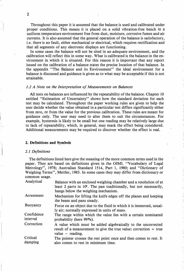
Throughout this paper it is assumed that the balance is used and calibrated under proper conditions. This means it is placed on a solid vibration-free bench in a uniform temperature environment free from dust, moisture, corrosive fumes and air currents. It is also assumed that the general operation of the balance is satisfactory, i.e. there is no fault, either mechanical or electrical, which requires rectification andthat all segments of any electronic displays are functioning.

In some cases the balance will not be sited in an adequate environment, and the calibration will reflect this in some way. What is calibrated is the balance in the en­vironment in which it is situated. For this reason it is important that any report issued on the calibration of a balance states the precise location of that balance. In the appendix "The Balance and its Environment" the ideal environment for a balance is discussed and guidance is given as to what may be acceptable if this is not attainable.

1.2 A Note on the Interpretation of Measurements on Balances

All tests on balances are influenced by the repeatability of the balance. Chapter 10 entitled "Estimation of Uncertainty" shows how the standard deviation for each test may be calculated. Throughout the paper working rules are given to help the user decide whether the value obtained in a particular test differs significantly either from zero, or from the value for the previous calibration. These rules are meant for guidance only. The user may need to alter them to suit the circumstances. For example, hysteresis is likely to be small but one reading may be relatively large due to lack of repeatability, which, in general, may mask the effect being considered. Additional measurements may be required to discover whether the effect is real.

2. Definitions and Symbols·

2.1 Definitions

The definitions listed here give the rrieaning of the more common terms used in the paper. They are based on definitions given in the OIML "Vocabulary of Legal Metrology", 1978; Australian Standard 1514, Part 1, 1980; and "Dictionary of Weighing Terms", Mettler, 1983. In some cases they may differ from dictionary or common usage. Analytical

Arrestment

Buoyancy

Confidence interval Correction

Critical damping

Balance with an enclosed weighing chamber and a resolution of at least 2 parts in 106

• The pan traditionally, but not necessarily, hangs below the weighing mechanism. Mechanism for lifting the knife edges off the planes and keeping the beam and pans steady. Force on an object due to the fluid in which it is immersed, usual­ly air; normally expressed in units of mass. The range within which the value lies with a certain nominated probability (here 99%). A value which must be added algebraically to the uncorrected result of a measurement to give the true value: correction = true value - reading. The pointer crosses the rest point once and then comes to rest. It also comes to rest in minimum time.

Damping

Decade

Departure from nominal value

Dial reading or setting

Digit Discrimination or resolution Double weighing

Error

Heel and toe

Hysteresis

Mass

Repeatability

Residual

Rest point

Scale

Scale division or interval Scale value

3

Means by which the motion of a swinging balance is brought to rest. Group of four masses from which any integral value from 1 to 10 may be formed using various combinations. The amount by which the reading on an instrument departs from its correct, or nominal, value. It is numerically equal to the cor­rection, but is opposite in sign. The digital reading on a mechanical dial used to indicate the value of the mass lifted off the beam for a single-pan balance, or ap­plied to the beam for a two-pan balance. Smallest unit of a digital readout. The smallest change in mass which can be detected by the balance.

Weighing procedure in which the standard and unknown are plac­ed one on each pan of a two-pan balance and then interchanged after reading. The difference between the two masses is half the difference between the two readings. Amount by which a reading departs from the true value: error = reading - true value. That is, error is the negative value of the correction and is therefore equal to the departure from nominal value. The term used when a knife edge contacts a plane without being parallel to it before contact. The difference between the indications of a measuring instrument when the same value of the quantity measured is reached by in­creasing or decreasing that quantity. The amount of matter in a body. This is an intrinsic property and is independent of physical changes, such as gravity, temperature etc. An object has a mass value measured in kilograms. Such an object is sometimes called a 'weight' (q.v.). The closeness of the agreement between the results of successive measurements of the same quantity carried out by the same method by the same observer at quit� short intervals of time. The difference between the calculated value and the observed value of a quantity. The reading a balance would display if the beam stopped swinging and came to rest. This is .usually measured as a function of the turning points without letting the balance come to rest. It is also called the centre of swing. ------1

�---

An ordered set of gauge or scale marks carried by the indicl.lji11�/ device of the balance. The means by which a mechanical or optical poi,..• deflection of the beam. The interval between two adjacent scale

For single-pan balances, the value of the b is close to its nominal value at full scale.

2

Throughout this paper it is assumed that the balance is used and calibrated under proper conditions. This means it is placed on a solid vibration-free bench in a uniform temperature environment free from dust, moisture, corrosive fumes and air currents. It is also assumed that the general operation of the balance is satisfactory, i.e. there is no fault, either mechanical or electrical, which requires rectification andthat all segments of any electronic displays are functioning.

In some cases the balance will not be sited in an adequate environment, and the calibration will reflect this in some way. What is calibrated is the balance in the en­vironment in which it is situated. For this reason it is important that any report issued on the calibration of a balance states the precise location of that balance. In the appendix "The Balance and its Environment" the ideal environment for a balance is discussed and guidance is given as to what may be acceptable if this is not attainable.

1.2 A Note on the Interpretation of Measurements on Balances ·

All tests on balances are influenced by the repeatability of the balance. Chapter 10 entitled "Estimation of Uncertainty" shows how the standard deviation for each test may be calculated. Throughout the paper working rules are given to help the user decide whether the value obtained in a particular test differs significantly either from zero, or from the value for the previous calibration. These rules are meant for guidance only. The user may need to alter them to suit the circumstances. For example, hysteresis is likely to be small but one reading may be relatively large due to lack of repeatability, which, in general, may mask the effect being considered. Additional measurements may be required to discover whether the effect is real.

2. Definitions and Symbols

2.1 Definitions

The definitions listed here give the meaning of the more common terms used in the paper. They are based on definitions given in the OIML "Vocabulary of Legal Metrology", 1978; Australian Standard 1514, Part 1, 1980; and "Dictionary of Weighing Terms", Mettler, 1983. In some cases they may differ from dictionary or common usage. Analytical

Arrestment

Buoyancy

Confidence interval

Correction

Critical damping

Balance with an enclosed weighing chamber and a resolution of at least 2 parts in 106

• The pan traditionally, but not necessarily, hangs below the weighing mechanism.

Mechanism for lifting the knife edges off the planes and keeping the beam and pans steady.

Force on an object due to the fluid in which it is immersed, usual­ly air; normally expressed in units of mass. The range within which the value lies with a certain nominated probability (here 99%).

A value which must be added algebraically to the uncorrected result of a measurement to give the true value: correction = true value - reading. The pointer crosses the rest point once and then comes to rest. It also comes to rest in minimum time.

Damping

Decade

Departure from nominal value

Dial reading or setting

Digit

Discrimination or resolution

Double weighing

Error

Heel and toe

Hysteresis

Mass

Repeatability

Residual

Rest point

Scale

Scale division or interval

Scale value

3

Means by which the motion of a swinging balance is brought to rest.

Group of four masses from which any integral value from 1 to 10 may be formed using various combinations.

The amount by which the reading on an instrument departs from its correct, or nominal, value. It is numerically equal to the cor­rection, but is opposite in sign.

The digital reading on a mechanical dial used to indicate the value of the mass lifted off the beam for a single-pan balance, or ap­plied to the beam for a two-pan balance.

Smallest unit of a digital readout.

The smallest change in mass which can be detected by the balance.

Weighing procedure in which the standard and unknown are plac­ed one on each pan of a two-pan balance and then interchanged after reading. The difference between the two masses is half the difference between the two readings.

Amount by which a reading departs from the true value: error = reading - true value. That is, error is the negative value of the correction and is therefore equal to the departure from nominal value.

The term used when a knife edge contacts a plane without being parallel to it before contact.

The difference between the indications of a measuring instrument when the same value of the quantity measured is reached by in­creasing or decreasing that quantity.

The amount of matter in a body. This is an intrinsic property and is independent of physical changes, such as. gravity, temperature etc. An object has a mass value measured in kilograms. Such an object is sometimes called a 'weight' (q.v.).

The closeness of the agreement between the results of successive measurements of the same quantity carried out by the same method by the same observer at quite short intervals of time.

The difference between the calculated value and the observed value of a quantity.

The reading a balance would display if the beam stopped swinging and came to rest. This is usually measured as a function of the turning points without letting the balance come to rest. It is also called the centre of swing.

An ordered set of gauge or scale marks carried by the indicating device of the balance. The means by which a mechanical or optical pointer indicates the deflection of the beam.

The interval between two adjacent scale marks.

For single-pan balances, the value of the balance reading when it is close to its nominal value at full scale.

I!

4

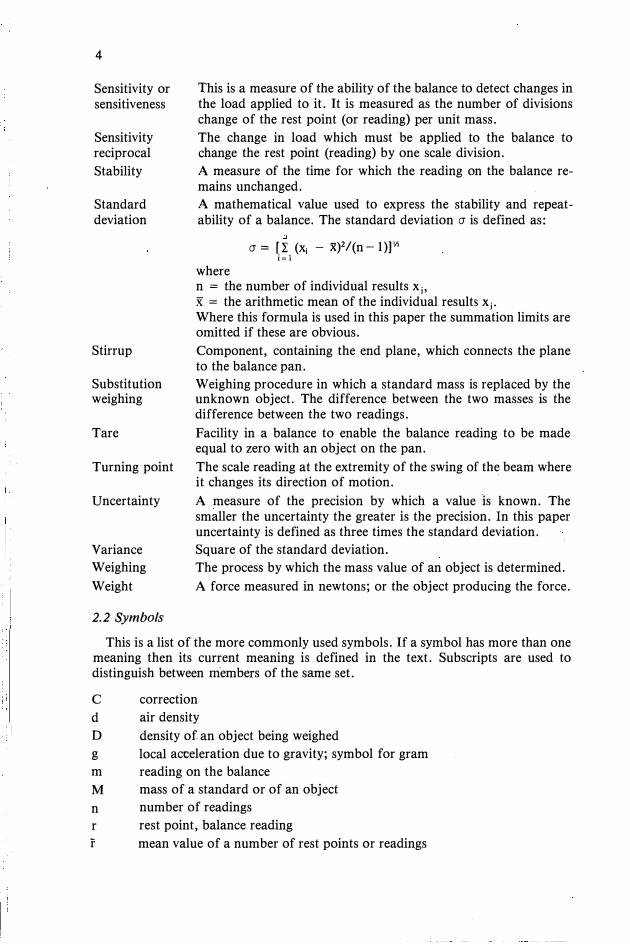
Sensitivity or sensitiveness

Sensitivity reciprocal

Stability

Standard deviation

Stirrup

Substitution weighing

Tare

Turning point

Uncertainty

Variance

Weighing

Weight

2.2 Symbols

This is a measure of the ability of the balance to detect changes in the load applied to it. It is measured as the number of divisions change of the rest point (or reading) per unit mass.

The change in load which must be applied to the balance to change the rest point (reading) by one scale division.

A measure of the time for which the reading on the balance re­mains unchanged.

A mathematical value used to express the stability and repeat­ability of a balance. The standard deviation a is defined as:

a= [I (xi - x)2/(n-1))\-> i=l

where n = the number of individual results x i, x = the arithmetic mean of the individual results x i. Where this formula is used in this paper the summation limits are omitted if these are obvious.

Component, containing the end plane, which connects the plane to the balance pan.

Weighing procedure in which a standard mass is replaced by the unknown object. The difference between the two masses is the difference between the two readings.

Facility in a balance to enable the balance reading to be made equal to zero with an object on the pan.

The scale reading at the extremity of the swing of the beam where it changes its direction of motion.

A measure of the precision by which a value is known. The smaller the uncertainty the greater is the precision. In this paper uncertainty is defined as three times the standard deviation.

Square of the standard deviation.

The process by which the mass value of an object is determined.

A force measured in newtons; or the object producing the force.

This is a list of the more commonly used symbols. If a symbol has more than one meaning then its current meaning is defined in the text. Subscripts are used to distinguish between members of the same set.

C

d

D

g

m

correction

air density

density of an object being weighed

local acceleration due to gravity; symbol for gram

reading on the balance

M mass of a standard or of an object

n number of readings

r

r

rest point, balance reading

mean value of a number of rest points or readings

5

s residual

s sum of squares of residuals

SR sensitivity reciprocal

SS stainless steel

t turning point

T manufacturer's tolerance

u uncertainty = 3 a

V volume of an object being weighed

z zero reading on the balance

a standard deviation

3. Types of Balances

Balances can be classified into the three categories described in this chapter.

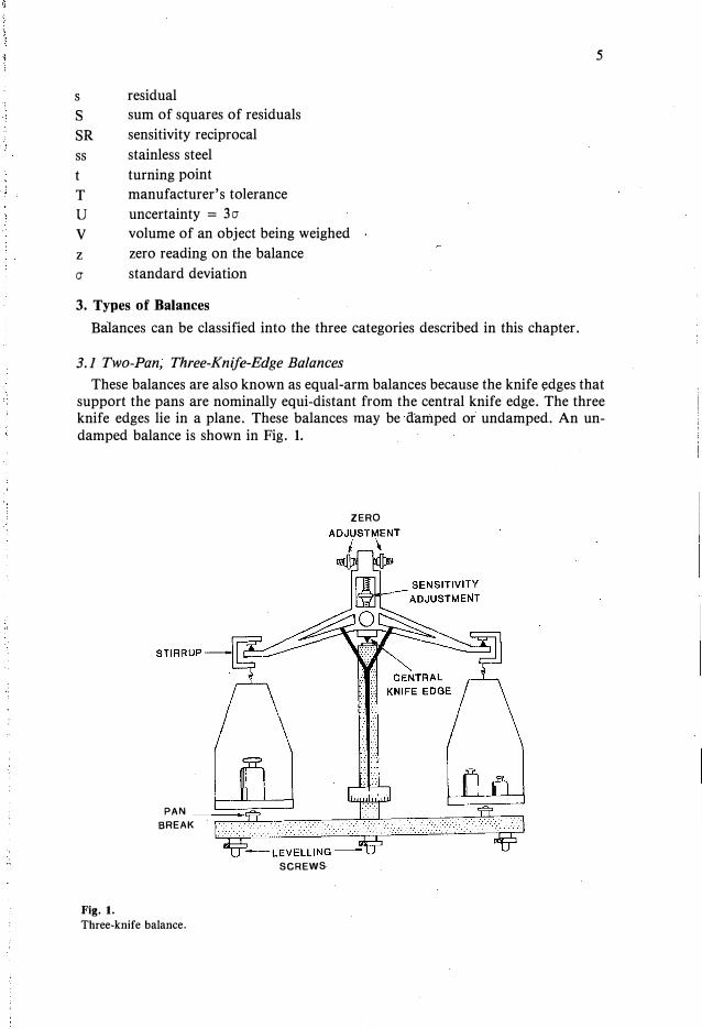
3.1 Two-Pan, Three-Knife-Edge Balances

These balances are also known as equal-arm balances because the knife edges that support the pans are nominally equi-distant from the central knife edge. The three knife edges lie in a plane. These balances may be a-amped or undamped. An un­damped balance is shown in Fig. 1.

ZERO

Fig. I.

Three-knife balance.

I

4

Sensitivity or sensitiveness

Sensitivity reciprocal

Stability

Standard deviation

Stirrup

Substitution weighing

Tare

Turning point

Uncertainty

Variance

Weighing

Weight

2.2 Symbols

This is a measure of the ability of the balance to detect changes in the load applied to it. It is measured as the number of divisions change of the rest point (or reading) per unit mass.

The change in load which must be applied to the balance to change the rest point (reading) by one scale division.

A measure of the time for which the reading on the balance re­mains unchanged.

A mathematical value used to express the stability and repeat­ability of a balance. The standard deviation CJ is defined as:

CJ= [I (xi - x)2/(n-1))\1 i=I

where n = the number of individual results x i, x = the arithmetic mean of the individual results x i. Where this formula is used in this paper the summation limits are omitted if these are obvious.

Component, containing the end plane, which connects the plane to the balance pan.

Weighing procedure in which a standard mass is replaced by the unknown object. The difference between the two masses is the difference between the two readings.

Facility in a balance to enable the balance reading to be made equal to zero with an object on the pan.

The scale reading at the extremity of the swing of the beam where it changes its direction of motion.

A _measure of the precision by which a value is known. The smaller the uncertainty the greater is the precision. In this paper uncertainty is defined as three times the standard deviation.

Square of the standard deviation.

The process by which the mass value of an object is determined.

A force measured in newtons; or the object producing the force.

This is a list of the more commonly used symbols. If a symbol has more than one meaning then its current meaning is defined in the text. Subscripts are used to distinguish between members of the same set.

C correction

d air density

D density of an object being weighed

g local acceleration due to gravity; symbol for gram

m reading on the balance

M mass of a standard or of an object

n number of readings

r rest point, balance reading

r mean value of a number of rest points or readings

5

s residual

s sum of squares of residuals

SR sensitivity reciprocal

SS stainless steel

t turning point

T manufacturer's tolerance

u uncertainty = 3 CJ

V volume of an object being weighed

z zero reading on the balance

(J standard deviation

3. Types of Balances

Balances can be classified into the three categories described in this chapter.

3.1 Two-Pan, Three-Knife-Edge Balances

These balances are also known as equal-arm balances because the knife edges that support the pans are nominally equi-distant from the central knife edge. The three knife edges lie in a plane. These balances may be a-amped or undamped. An un­damped balance is shown in Fig. 1.

ZERO

PAN

BREAK

SCREWS

Fig. 1.

Three-knife balance.

I

! i

6

The theory and use of three-knife-edge balances are described by Glazebrook (1950) and NPL (1954). 3.1.1 Damped balances

The damping medium is usually air, but may be oil or a magnetic field. Damping is usually arranged to be critical, i.e. the pointer crosses the rest point once and then comes to rest. Damped balances usually have a light and projection system to image a scale, attached to the end of the pointer, onto a screen in the front of the balance. The sensitivity of the balance is adjusted to make the scale divisions equal to some nominal value. 3.1.2 Undamped or free-swinging balances

These )Jalances are subject to slight natural damping, which is so small that it is not practicable to wait for the balance to come to rest to determine the rest point. In &eneral the centre of swing or rest point is obtained from readings of the turning points. There are a number of formulae used for calculating the rest point. AU are biased to a very small extent, but this bias is negligible unless the damping is fairly large (Bignell, 1983). Any bias largely cancels out even for large damping, because the result is the difference between two rest points. The usual formula used for calculating the rest point is

(1)

where t1 •••• t5 are successive values of the turning point. Because dynamic friction is smaller than static friction, undamped balances are

more sensitive than damped balances, but they are not as convenient to use.

3.2 Single-Pan, Two-Knife-Edge Balances

These instrument$ fall into two categories usually termed top-loading and analytical balances. A diagram of an analytical balance is given in Fig. 2. In the

Fig. 2.

HANGER AND

BUILT-IN MASSES-

SCREW

Single-pan constant-load analytical balance.

_SENSITIVITY ADJUSTMENT

AIR

r

'

7

analytical balance the load is suspended below the balance beam and the beam is ar­rested during loading and unloading of the pan. For the top-loading balance the pan is supported above the beam by a parallelogram linkage and there is usually no ar­resting mechanism. Both types of balances are almost always critically damped. Most balances have built-in masses attached to the pan assembly so that whenever a load is placed on the pan an equivalent mass is lifted from the pan, thus ensuring that the reading remains within the optical range of the balance. This means that the mass to be supported by the knife edges in the balance is fairly constant, so balances of this type are often referred to as constant-load balances. Also the sensitivity is unlikely to vary with load. The traditional optical display is sometimes replaced with an electronic digital display, but this does not affect the method of testing and use.

Due to their construction it is often very difficult to measure the parallelism of the knife edges of these balances. The knife edges are usually glued to the beam with no adjustment provided, the alignment being pre-set by the manufacturer.

Balances which may have means other than knife edges for supporting the beam (e.g. flexure pivots), may be tested by the methods outlined.

3. 3 Electromagnetic-Force-Compensation Balances

All balances of this type measure the total gravitational force, or weight, ratherthan compare forces, and this determines the form of the balance. Figure 3 shows

Fig. 3.

AID

CONVERTER

MICRO­

PROCESSOR

Basic diagram of an electromagnetic-force-compensated balance.

WEIGHING PAN

DISPLAY

6

The theory and. use of three-knife-edge balances are described by Glazebrook (1950) and NPL (1954).

3.1.1 Damped balances The damping medium is usually air, but may be oil or a magnetic field. Damping

is usually arranged to be critical, i.e. the pointer crosses the rest point once and then comes to rest. Damped balances usually have a light and projection system to image a scale, attached to the end of the pointer, onto a screen in the front of the balance. The sensitivity of the balance is adjusted to make the scale divisions equal to some nominal value. 3.1.2 Undamped or free-swinging balances

These )Jalances are subject to slight natural damping, which is so small that it is not practicable to wait for the balance to come to rest to determine the rest point. In &eneral the centre of swing or rest point is obtained from readings of the turning points. There are a number of formulae used for calculating the rest point. All are biased to a very small extent, but this bias is negligible unless the damping is fairly large (Bignell, 1983). Any bias largely cancels out even for large damping, because the result is the difference between two rest points. The usual formula used for calculating the rest point is

(1)

where t1 • • • • t5 are successive values of the turning point. Because dynamic friction is smaller than static friction, undamped balances are

more sensitive than damped balances, but they are not as convenient to use.

3.2 Single-Pan, Two-Knife-Edge Balances

These instrument� fall into two categories usually termed top-loading and analytical balances. A diagram of an analytical balance is given in Fig. 2. In the

Fig. 2.

HANGER AND

BUILT-IN MASSES�

SCREW

Single-pan constant-load analytical balance.

AIR

DAMPING

l 7

analytical balance the load is suspended below the balance beam and the beam is ar­rested during loading and unloading of the pan. For the top-loading balance the pan is supported above the beam by a parallelogram linkage and there is usually no ar­resting mechanism. Both types of balances are almost always critically damped. Most balances have built-in masses attached to the pan assembly so that whenever a load is placed on the pan an equivalent mass is lifted from the pan, thus ensuring that the reading remains within the optical range of the balance. This means that the mass to be supported by the knife edges in the balance is fairly constant, so balances of this type are often referred to as constant-load balances. Also the sensitivity is unlikely to vary with load. The traditional optical display is sometimes replaced with an electronic digital display, but this does not affect the method of testing and use.

Due to their construction it is often very difficult to measure the parallelism of the knife edges of these balances. The knife edges are usually glued to the beam with no adjustment provided, the alignment being pre-set by the manufacturer.

Balances which may have means other than knife edges for supporting the beam (e.g. flexure pivots), may be tested by the methods outlined.

3.3 Electromagnetic-Force-Compensation Balances

All balances of this type measure the total gravitational force, or weight, rather than compare forces, and this determines the form of the balance. Figure 3 shows

COIL

Fig. 3.

AID

CONVERTER

MICRO­

PROCESSOR

Basic diagram of an electromagnetic-force-compensated balance.

WEIGHING PAN

DISPLAY

8

the principle of the balance. Because of their construction most are top-loading balances. A coil, rigidly attached to the balance pan, is placed in the annular gap of a magnet. When a mass is added to the pan a position sensor detects that the pan has been lowered and causes a current through the coil to be increased, providing a magnetic counter-force which returns the balance pan to the original position. The compensating current is measured as a voltage across a resistor R and then is read out on what is effectively a digital voltmeter. The compensating current is in direct proportion to the mass on the pan, and hence the actual value of the mass may be obtained. As the main operation of the balance is electrical/ electronic rather than opto-mechanical, they are often called electronic balances.

Some analytical balances are specially designed so that the weighing is done below the force cell. With precision amplifiers, changes in force of 3 parts in 107 can be detected, but typical analytical balances are produced with discriminations of 6 parts in 107

• Because the display of this type of balance can be zeroed at any load by the touch of a button, no special taring facility is required.

A number of large capacity balances, particularly platform scales, have strain­gauge load cells as the sensing mechanism. At present these balances are limited to an accuracy of about 1 part in 104. However because electronic balances can be con­sidered as black boxes the method of calibration is independent of the system used to detect the mass.

4. Calibration of Two-Pan, Three-Knife-Edge Balances

4.1 Repeatability of Reading

Repeatability is a measure of how well a balance will weigh. Ultimately all the other tests are to ensure that the correct mass value is obtained. The repeatability is normally expressed· in terms of the standard deviation obtained from a series of repeated readings together with the relative size of the maximum difference between two successive readings. For a good balance neither of these should be more than twice the discrimination. However· the readings must be obtained in a way that realistically simulates how the balance is used in practice. The following methods are all used but only those outlined in section (c) are recommended. Those of sections (a) and (b) are useful for checking that the performance of the balance has notchanged. Measurements should be made at a number of different loads becausethese often give larger values of the standard deviation than readings made at zeroload.

(a) The balance is released and the rest point, r1 noted. This is repeated n times(n ) 10) and the standard deviation calculated by means of the formula.

o- == [ I (r i - f)2/(n -l)P' i == 1, ... ,n. (2)

(b) An extension of this formula is obtained by taking rest point readings (ai, ck

and bj) near each end of the scale and the centre respectively, and combining the

three sets in the following formula:

()' ==

[ P Q _ R ]Yi I(a;-a)2 +I (bi- b)2 +I (ck -c)2

I I I (P-1) + (Q

i == l, .. ,P j == 1, .. ,Q k == 1, .. ,R

(3)

9

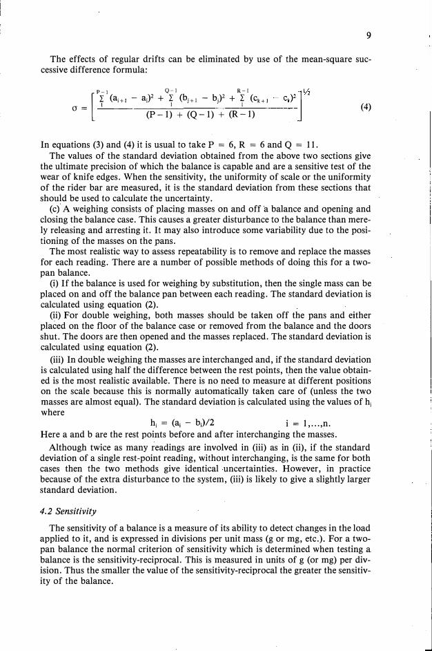
The effects of regular drifts can be eliminated by use of the mean-square suc­cessive difference formula:

P-1 Q-1 R-1

[ I (ai+1 - ai)2 + I (bi+I - bi)2 + I (ck+I

1 1 1 er == (P -1) + (Q-1) + (R -1)

In equations (3) and (4) it is usual to take P == 6, R == 6 and Q == 11.

(4)

The values of the standard deviation obtained from the above two sections give the ultimate precision of which the balance is capable and are a sensitive test of the wear of knife edges. When the sensitivity, the uniformity of scale or the uniformity of the rider bar are measured, it is the standard deviation from these sections that should be used to calculate the uncertainty.

(c)' A weighing consists of placing masses on and off a balance and opening and closing the balance case. This causes a greater disturbance to the balance than mere­ly releasing and arresting it. It may also introduce some variability due to the posi­tioning of the masses on the pans.

The most realistic way to assess repeatability is to remove and replace the masses for each reading. There are a number of possible methods of doing this for a two­pan balance. · (i) If the balance is used for weighing by substitution, then the single mass can beplaced on and off the balance pan between each reading. The standard deviation iscalculated using equation (2).

(ii) For double weighing, both masses should be taken off the pans and eitherplaced on the floor of the balance case or removed from the balance and the doors shut. The doors are then opened and the masses replaced. The standard deviation is calculated using equation (2).

(iii) In double weighing the masses are interchanged and, if the standard deviationis calculated using half the difference between the rest points, then the value obtain­ed is the most realistic available. There is no need to measure at different positions on the scale because this is normally automatically taken care of (unless the two masses are almost equal). The standard deviation is calculated using the values of hi

where hi == (a; - b)/2 i == 1, ... ,n.

Here a and b are the rest points before and after interchanging the masses. Although twice as many readings are involved in (iii) as in (ii), if the standard

deviation of a single rest-point reading, without interchanging, is the same for both cases then the two methods give identical uncertainties. However, in practice because of the extra disturbance to the system, (iii) is likely to give a slightly larger standard deviation.

4.2 Sensitivity

The sensitivity of a balance is a measure of its ability to detect changes in the load applied to it, and is expressed in divisions per unit mass (g or mg, etc.). For a two­pan balance the normal criterion of sensitivity which is determined when testing a balance is the sensitivity-reciprocal. This is measured in units of g (or mg) per div­ision. Thus the smaller the value of the sensitivity-reciprocal the greater the sensitiv­ity of the balance.

: I

I 'I

.,

8

the principle of the balance. Because of their construction most are top-loading balances. A coil, rigidly attached to the balance pan, is placed in the annular gap of a magnet. When a mass is added to the pan a position sensor detects that the pan has been lowered and causes a current through the coil to be increased, providing a magnetic counter-force which returns the balance pan to the original position. The compensating current is measured as a voltage across a resistor R and then is read out on what is effectively a digital voltmeter. The compensating current is in direct proportion to the mass on the pan, and hence the actual value of the mass may be obtained. As the main operation of the balance is electrical/electronic rather than opto-mechanical, they are often called electronic balances.

Some analytical balances are specially designed so that the weighing is done below the force cell. With precision amplifiers, changes in force of 3 parts in 107 can be detected, but typical analytical balances are produced with discriminations of 6 parts in 107

• Because the display of this type of balance can be zeroed at any load by the touch of a button, no special taring facility is required.

A number of large capacity balances, particularly platform scales, have strain­gauge load cells as the sensing mechanism. At present these balances are limited to an accuracy of about 1 part in 104. However because electronic balances can be con­sidered as black boxes the method of calibration is independent of the system used to detect the mass.

4. Calibration of Two-Pan, Three-Knife-Edge Balances

4.1 Repeatability of Reading

Repeatability is a measure of how well a balance will weigh. Ultimately all the other tests are to ensure that the correct mass value is obtained. The repeatability is normally expressed· in terms of the standard deviation obtained from a series of repeated readings together with the relative size of the maximum difference between two successive readings. For a good balance neither of these should be more than twice the discrimination. However· the readings must be obtained in a way that realistically simulates how the balance is used in practice. The following methods are all used but only those outlined in section (c) are recommended. Those of sections (a) and (b) are useful for checking that the performance of the balance has notchanged. Measurements should be made at a number of different loads becausethese often give larger values of the standard deviation than readings made at zeroload.

(a) The balance is released and the rest point, r1 noted. This is repeated n times(n ) 10) and the standard deviation calculated by means of the formula.

a = [ I (ri - f)2/(n - l)P'2 i = 1, ... ,n. (2)

(b) An extension of this formula is obtained by taking rest point readings (ai, ck

and bj) near each end of the scale and the centre respectively, and combining the three sets in the following formula:

a

[ P Q _ R l\/2

I(a, - a)2 + I (bi - b)2 + I (ck - c)2

I I I

(P -1) + (Q-1) + (R-1)

i = 1, .. ,P j = 1, .. ,Q (3) k = 1, .. ,R

9

The effects of regular drifts can be eliminated by use of the mean-square suc­cessive difference formula:

P-1 Q-1 R-1

[ I (ai+1 - aY + I (bi+1 - b

j)2 + I (ck +1

I I I CJ =

(P - 1) + (Q- 1) + (R - 1)

In equations (3) and (4) it is usual to take P = 6, R = 6 and Q = 11.

(4)

The values of the standard deviation obtained from the above two sections give the ultimate precision of which the balance is capable and are a sensitive test of the wear of knife edges. When the sensitivity, the uniformity of scale or the uniformity of the rider bar are measured, it is the standard deviation from these sections that should be used to calculate the uncertainty.

(cf A weighing consists of placing masses on and off a balance and opening and closing the balance case. This causes a greater disturbance to the balance than mere­ly releasing and arresting it. It may also introduce some variability due to the posi­tioning of the masses on the pans.

The most realistic way to assess repeatability is to remove and replace the masses for each reading. There are a number of possible methods of doing this for a two­pan balance. · (i) If the balance is used for weighing by substitution, then the single mass can beplaced on and off the balance pan between each reading. The standard deviation iscalculated using equation (2).

(ii) For double weighing, both masses should be taken off the pans and eitherplaced on the floor of the balance case or removed from the balance and the doors shut. The doors are then opened and the masses replaced. The standard deviation is calculated using equation (2).

(iii) In double weighing the masses are interchanged and, if the standard deviationis calculated using half the difference between the rest points, then the value obtain­ed is the most realistic available. There is no need to measure at different positions on the scale because this is normally automatically taken care of (unless the two masses are almost equal). The standard deviation is calculated using the values of hi

where hi = (ai - b)/2 i = 1, ... ,n.

Here a and b are the rest points before and after interchanging the masses. Although twice as many readings are involved in (iii) as in (ii), if the standard

deviation of a single rest-point reading, without interchanging, is the same for both cases then the two methods give identical uncertainties. However, in practice because of the extra disturbance to the system, (iii) is likely to give a slightly larger standard deviation.

4.2 Sensitivity

The sensitivity of a balance is a measure of its ability to detect changes in the load applied to it, and is expressed in divisions per unit mass (g or mg, etc.). For a two­pan balance the normal criterion of sensitivity which is determined when testing a balance is the sensitivity-reciprocal. This is measured in units of g (or mg) per div­ision. Thus the smaller the value of the sensitivity-reciprocal the greater the sensitiv­ity of the balance.

10

Since it is usual for the value of the sensitivity-reciprocal to change significantly when the loading is varied its value should be determined for several different loads - usually zero, half-maximum and maximum. This change occurs when the threeknife-edges are not co-planar and generally is attributable either to imperfect align­ment of the knife edges or to bending of the beam. A variation with load of up to200Jo in the value of the sensitivity-reciprocal is generally acceptable. For high pre­cision weighing the sensitivity-reciprocal should be measured for each load at whichthe balance is used.

For a damped balance the sensitivity is determined by adding a known mass, equal to the nominal range of the scale, to the appropriate pan. For an undamped balance a mass equal to about a quarter of the range of the scale is most convenient. A balance· is made more sensitive (i.e. the sensitivity-reciprocal is decreased) by raising the centre of gravity of the beam. To enable this to be done easily most balances have a small nut on a vertical threaded rod at the centre of the beam.

4.3 Parallelism of Knife Edges

It is more important for knife edges to be parallel and co-planar than for the arm lengths to be equal. If the knife edges are not parallel then any shift in the point of application of the load will change the rest point. This can happen if the position of the load on the pan is altered, although for a well constructed pan support system this will be small. However friction will still cause positioning of the load to have some effect.

Parallelism of the knife edges can be measured in plan view by replacing the pan­support plane with a plane of about a quarter to a half its length. An arm is attached to the plane so that a load M can be applied to the knife edge. The change in rest point is measured as the plane is moved from the front to the back of the knife edge. Most pan-support knife edges are fitted with small screws to enable each knife edge to be adjusted parallel to the central knife edge.

Small planes are not readily obtainable or easily mounted appropriately, and so an alternative procedure is as follows. A small mass or piece of metal, M, is chosen that will safely sit on the top of the pan-support plane. The mass is moved from the front to the back of the plane and the change in the rest point is observed. When this is done according to the observation scheme set out in Table 1 a mass of value M should be added to the other balance pan.

There are two errors due to misalignment in the vertical plane (or side view). (a) If the knives are parallel with respect to the horizontal but not co-planar then thesensitivity will change with load (section 4.2).(b) Tilt of the knives in the vertical plane with respect to the central knife edge canhave two effects. Firstly, the pans will kick as the knives come into contact with theplanes - sometimes called heel and toe error. Secondly, the sensitivity will change inthe same manner as the rest point does for the shift error (section 4. 7).

Usually, there are no adjustments on the balance to correct these faults, but they can be eliminated by shimming. For a good balance any errors of these types should be within the discrimination. This can be determined by use of the small plane described above, but not by moving the masses on top of the plane (see below).

One of the easiest methods of measuring the amount of shimming required is to remove the beam from the balance, place it upside down on a surface plate with the two end knives supported on gauge block combinations of equal height. The height

11

of the central knife edge may then be measured by use of another gauge block com­bination.

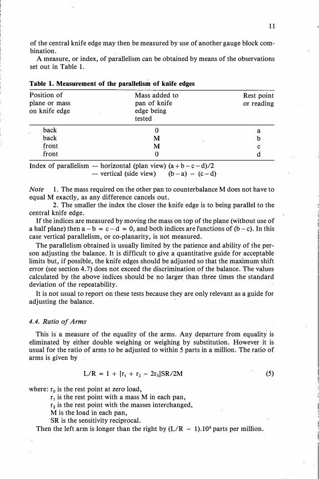
A measure, or index, of parallelism can be obtained by means of the observations set out in Table 1.

Table 1. Measurement of the parallelism of knife edges

Position of plane or mass on knife edge

back back front front

Mass added to pan of knife edge being tested

0 M M 0

Index of parallelism - horizontal (plan view) (a+ b - c - d)/2 - vertical (side view) (b - a) - (c - d)

Rest point or reading

a b C

d

Note 1. The mass required on the other pan to counterbalance M does not have to equal M exactly, as any difference cancels out.

2. The smaller the index the closer the knife edge is to being parallel to thecentral knife edge.

If the indices are measured by moving the mass on top of the plane (without use of a half plane) then a - b = c - d = 0, and both indices are functions of (b - c).In this case vertical parallelism, or co-planarity, is not measured.

The parallelism obtained is usually limited by the patience and ability of the per­son adjusting the balance. It is difficult to give a quantitative guide for acceptable limits but, if possible, the knife edges should be adjusted so that the maximum shift error (see section 4. 7) does not exceed the discrimination of the balance. The values calculated by the above indices should be no larger than three times the standard deviation of the repeatability.

It is not usual to report on these tests because they are only relevant as a guide for adjusting the balance.

4. 4. Ratio of Arms

This is a measure of the equality of the arms. Any departure from equality iseliminated by either double weighing or weighing by substitution. However it is usual for the ratio of arms to be adjusted to within 5 parts in a million. The ratio of arms is given by

L/R = 1 + [r1 + r2 - 2r0]SR/2M (5)

where: r0 is the rest point at zero load, r1 is the rest point with a mass M in each pan, r2 is the rest point with the masses interchanged,M is the load in each pan, SR is the sensitivity reciprocal.

Then the left arm is longer than the right by (L/R - 1).106 parts per million.

j

I

10

Since it is usual for the value of the sensitivity-reciprocal to change significantly when the loading is varied its value should be determined for several different loads - usually zero, half-maximum and maximum. This change occurs when the threeknife-edges are not co-planar and generally is attributable either to imperfect align­ment of the knife edges or to bending of the beam. A variation with load of up to20% in the value of the sensitivity-reciprocal is generally acceptable. For high pre­cision weighing the sensitivity-reciprocal should be measured for each load at whichthe balance is used.

For a damped balance the sensitivity is determined by adding a known mass, equal to the nominal range of the scale, to the appropriate pan. For an undamped balance a mass equal to about a quarter of the range of the scale is most convenient. A balance is made more sensitive (i.e. the sensitivity-reciprocal is decreased) by raising the centre of gravity of the beam. To enable this to be done easily most balances have a small nut on a vertical threaded rod at the centre of the beam.

4. 3 Parallelism of Knife Edges

It is more important for knife edges to be parallel and co-planar than for the arm lengths to be equal. If the knife edges are not parallel then any shift in the point ofapplication of the load will change the rest point. This can happen if the position ofthe load on the pan is altered, although for a well constructed pan support systemthis will be small. However friction will still cause positioning of the load to havesome effect.

Parallelism of the knife edges can be measured in plan view by replacing the pan­support plane with a plane of about a quarter to a half its length. An arm is attachedto the plane so that a load M can be applied to the knife edge. The change in restpoint is measured as the plane is moved from the front to the back of the knife edge.Most pan-support knife edges are fitted with small screws to enable each knife edgeto be adjusted parallel to the central knife edge.

Small planes are not readily obtainable or easily mounted appropriately, and soan alternative procedure is as follows. A small mass or piece of metal, M, is chosenthat will safely sit on the top of the pan-support plane. The mass is moved from thefront to the back of the plane and the change in the rest point is observed. When thisis done according to the observation scheme set out in Table l a mass of value Mshould be added to the other balance pan.

There are two errors due to misalignment in the vertical plane (or side view). (a) If the knives are parallel with respect to the horizontal but not co-planar then thesensitivity will change with load (section 4.2).(b) Tilt of the knives in the vertical plane with respect to the central knife edge canhave two effects. Firstly, the pans will kick as the knives come into contact with theplanes - sometimes called heel and toe error. Secondly, the sensitivity will change inthe same manner as the rest point does for the shift error (section 4. 7).

Usually, there are no adjustments on the balance to correct these faults, but they can be eliminated by shimming. For a good balance any errors of these types should be within the discrimination. This can be determined by use of the small plane described above, but not by moving the masses on top of the plane (see below).

One of the easiest methods of measuring the amount of shimming required is to remove the beam from the balance, place it upside down on a surface plate with the two end knives supported on gauge block combinations of equal height. The height

11

of the central knife edge may then be measured by use of another gauge block com­bination.

A measure, or index, of parallelism can be obtained by means of the observations set out in Table 1.

Table 1. Measurement of the parallelism of knife edges

Position of Mass aµded to plane or mass pan of knife on knife edge edge being

tested

back back front front

0

M

M

0

Index of parallelism - horizontal (plan view) (a+ b -c -d)/2 - vertical (side view) (b- a) - (c -d)

Rest point or reading

a b C

d

Note 1. The mass required on the other pan to counterbalance M does not have to equal M exactly, as any difference cancels out.

2. The smaller the index the closer the knife edge is to being parallel to thecentral knife edge.

If the indices are measured by moving the mass on top of the plane (without use ofa half plane) then a -b = c -d = 0, and both indices are functions of (b -c).In this case vertical parallelism, or co-planarity, is not measured.

The parallelism obtained is usually limited by the patience and ability of the per­son adjusting the balance. It is difficult to give a quantitative guide for acceptable limits but, if possible, the knife edges should be adjusted so that the maximum shift error (see section 4. 7) does not exceed the discrimination of the balance. The values calculated by the above indices should be no larger than three times the standard deviation of the repeatability.

It is not usual to report on these tests because they are only relevant as a guide for adjusting the balance.

4. 4. Ratio of Arms

This is a measure of the equality of the arms. Any departure from equality iseliminated by either double weighing or weighing by substitution. However it is usual for the ratio of arms to be adjusted to within 5 parts in a million. The ratio of arms is given by

L/R = 1 + [r1 + r2 - 2r0]SR/2M (5)

where: r0 is the rest point at zero load, r 1 is the rest point with a mass M in each pan, r2 is the rest point with the masses interchanged,M is the load in each pan, SR is the sensitivity reciprocal.

Then the left arm is longer than the right by (L/R - 1).106 parts per million.

12

Note. 1. The value of the sensitivity-reciprocal used in equation (5) is the value ob­tained with a load M on the balance.

2. For precision balances it is more important to have the knife edges parallelthan to have the arm lengths almost equal.

By differentiating equation (5) the standard deviation of the ratio of arms can be

obtained. This is given by

standard deviation = l.22CJ /M .106 parts per million, (6)

where CJ is the standard deviation obtained from the repeatability of reading and M is the n;iass used to measure the ratio of arms.

4.5 Uniformity of Scale

This test is sometimes termed linearity of response because the purpose is not to measure the uniformity of the scale but rather to check the effective shape of the knife edges. If the knife-edges are of irregular shape a change of load within the range of the scale will not be indicated as a proportional change in scale reading.

This amounts to the sensitivity-reciprocal varying with the scale reading. Irregularities in the scale reading should not amount to more than twice the

discrimination of the balance (or standard deviation for a sensitive balance). A value in excess of this would generally indicate defective knife-edges. It could also be at­tributed to irregular spacing of the scale marks, but this is most unlikely.

The uniformity should be determined at a number of points, usually 5, over the range of the scale by successively placing small calibrated masses on the pan ( or moving the rider along the bar) and observing the readings. From these readings the corrections are easily calculated. These measurements are normally done at half the maximum load of.the balance. The method is outlined in detail in sections 5 .3 .1 and 5-.3.2. It is possible, although inconvenient, to apply scale corrections when using a damped balance, but this is virtually impossible with an undamped balance.

4. 6 Rider Bar

Many two-pan balances are equipped with a rider bar. This enables smaller in­crements of mass than are available with fractional masses to be added to the pans. However, due to variable seating of the rider on the bar, use of the rider is not quite as accurate as calibrated masses. If the rider is used during weighing, then it should be left on the bar when at the zero position.

The bar is likely to be evenly graduated but the scale could be displaced relative to the knife edges. To test this a calibrated mass equal to the rider is placed on one pan and a counterpoise on the other. If the mass is removed and the rider placed on the bar then the difference in the rest points, after allowing for any difference between the mass of the rider and the calibrating mass, gives the error due to displacement of the rider bar. The resolution of this test may be increased by using a rider more than

ten times the nominal mass. Unless the rider bar is removed during an overhaul, this calibration should only

need to be done once during the life of the balance.

4. 7 Effect of Off-Centre Loading

This is also known as shift or corner-load error. It is important for top-loading

13

balances, but it is not normally measured on two-pan balances. As mentioned in sec­tion 4.3 it can be important for precise weighing. This effect is easily measured by placing a mass in the centre of the pan and then moving it to front, rear, left and right positions on the pan and noting any change in the reading. The mass should be moved sufficiently to ascertain that the accuracy of any weighings done on the balance will not be affected by the positioning of the load. Approximately a quarter of the pan radius is adequate. The amount moved should be sufficient so that the pan is obviously no longer horizontal but without it touching anything. This test should be carried out at approximately half the maximum load of the balance. Ac­curate masses are not required, any suitable piece of turned brass or stainless steel being adequate.

4. 8 Masses Associated with the Balance

Some damped balances have small masses that can be placed on a bar attached tothe pan suspension. The manipulation of the masses is performed from outside the balance case by means of a knob. These masses can be calibrated in two ways.

(a) The masses can usually be readily removed from the balance and then weighed

on another more sensitive balance. If this is done a brief test should be made to en­sure that the correct values are obtained after the masses have been returned to the

balance. (b) It is often preferable to leave the masses in the balance and calibrate them in

situ. In this case any small errors due to the positioning of the masses or the loading mechanism are effectively calibrated out of the system. The method is equivalent to weighing by substitution. With the mass to be calibrated lifted off the pan, a calibrated mass is placed on the same pan and a suitable counterpoise is placed on the other pan to bring the reading to zero. The reading is noted, the calibrated mass is removed from the pan, and the balance mass is lowered into position. The value of the mass is easily obtained from the difference in the readings and the known value of the calibrated mass. Where a number of masses may be placed on the pan in com­binations, greater accuracy may be obtained by a least-squares analysis as described in chapter 9.

It should be noted that the masses associated with these balances are of necessity always used on only one pan. This effectively limits the use of these masses to weighings performed by substitution.

4.9 The Balance Arrestment

While this is not an attribute that can be calibrated, malfunctioning of the arrest­ment mechanism is a possible cause of poor repeatability of reading. The purpose of the arrestment is to protect the knife edges during loading and unloading of the balance. In order to function properly the knives should make contact with their respective planes in exactly the same manner each time the balance is released and there must be no sudden or jerky movements on release.

The most common defect on operation of the beam arrestment is heel and toeing of the central knife on the plane. This occurs if the knife and plane are not parallel in the arrested position. One end of the knife then makes contact with the plane before the other. This can usually be detected by watching the beam for any sign of tilt as it is released.

The stirrup arrestments for the end knives may have various types of maladjust­ment. Heel and toe movements may occur as for the central knife. In addition,

12

Note. 1. The value of the sensitivity-reciprocal used in equation (5) is the value ob­tained with a load M on the balance.

2. For precision balances it is more important to have the knife edges parallelthan to have the arm lengths almost equal.

By differentiating equation (5) the standard deviation of the ratio of arms can be obtained. This is given by

standard deviation = 1.22a /M .106 parts per million, (6)

where a is the standard deviation obtained from the repeatability of reading and M is the n;iass used to measure the ratio of arms.

4.5 Uniformity of Scale

This test is sometimes termed linearity of response because the purpose is not to measure the uniformity of the scale but rather to check the effective shape of the knife edges. If the knife-edges are of irregular shape a change of load within the

range of the scale will not be indicated as a proportional change in scale reading. This amounts to the sensitivity-reciprocal varying with the scale reading.

Irregularities in the scale reading should not amount to more than twice the discrimination of the balance (or standard deviation for a sensitive balance). A value in excess of this would generally indicate defective knife-edges. It could also be at­tributed to irregular spacing of the scale marks, but this is most unlikely.

The uniformity should be determined at a number of points, usually 5, over the

range of the scale by successively placing small calibrated masses on the pan (or moving the rider along the bar) and observing the readings. From these readings the corrections are easily calculated. These measurements are normally done at half the maximum load of.the balance. The method is outlined in detail in sections 5. 3 .1 and 5-.3.2. It is possible, although inconvenient, to apply scale corrections when using a damped balance, but this is virtually impossible with an undamped balance.

4. 6 Rider Bar

Many two-pan balances are equipped with a rider bar. This enables smaller in­crements of mass than are available with fractional masses to be added to the pans. However, due to variable seating of the rider on the bar, use of the rider is not quite as accurate as calibrated masses. If the rider is used during weighing, then it should be left on the bar when at the zero position.

The bar is likely to be evenly graduated but the scale could be displaced relative to the knife edges. To test this a calibrated mass equal to the rider is placed on one pan and a counterpoise on the other. If the mass is removed and the rider placed on the

bar then the difference in the rest points, after allowing for any difference between the mass of the rider and the calibrating mass, gives the error due to displacement of the rider bar. The resolution of this test may be increased by using a rider more than ten times the nominal mass.

Unless the rider bar is removed during an overhaul, this calibration should only need to be done once during the life of the balance.

4. 7 Effect of Off-Centre Loading

This is also known as shift or corner-load error. It is important for top-loading

13

balances, but it is not normally measured on two-pan balances. As mentioned in sec­tion 4.3 it can be important for precise weighing. This effect is easily measured by

placing a mass in the centre of the pan and then moving it to front, rear, left and right positions on the pan and noting any change in the reading. The mass should be moved sufficiently to ascertain that the accuracy of any weighings done on the balance will not be affected by the positioning of the load. Approximately a quarter of the pan radius is adequate. The amount moved should be sufficient so that the pan is obviously no longer horizontal but without it touching anything. This test should be carried out at approximately half the maximum load of the balance. Ac­curate masses are not required, any suitable piece of turned brass or stainless steel being adequate.

4. 8 Masses Associated with the Balance

Some damped balances have small masses that can be placed on a bar attached tothe pan suspension. The manipulation of the masses is performed from outside the balance case by means of a knob. These masses can be calibrated in two ways.

(a) The masses can usually be readily removed from the balance and then weighed

on another more sensitive balance. If this is done a brief test should be made to en­sure that the correct values are obtained after the masses have been returned to the balance.

(b) It is often preferable to leave the masses in the balance and calibrate them insitu. In this case any small errors due to the positioning of the masses or the loading mechanism are effectively calibrated out of the system. The method is equivalent to weighing by substitution. With the mass to be calibrated lifted off the pan, a calibrated mass is placed on the same pan and a suitable counterpoise is placed on the other pan to bring the reading to zero. The reading is noted, the calibrated mass is removed from the pan, and the balance mass is lowered into position. The value of the mass is easily obtained from the difference in the readings and the known value of the calibrated mass. Where a number of masses may be placed on the pan in com­binations, greater accuracy may be obtained by a least-squares analysis as described in chapter 9.

It should be noted that the masses associated with these balances are of necessity always used on only one pan. This effectively limits the use of these masses to weighings performed by substitution.

4.9 The Balance Arrestment

While this is not an attribute that can be calibrated, malfunctioning of the arrest­ment mechanism is a possible cause of poor repeatability of reading. The purpose of the arrestment is to protect the knife edges during loading and unloading of the balance. In order to function properly the knives should make contact with their respective planes in exactly the same manner each time the balance is released and there must be no sudden or jerky movements on release.

The most common defect on operation of the beam arrestment is heel and toeing

of the central knife on the plane. This occurs if the knife and plane are not parallel in the arrested position. One end of the knife then makes contact with the plane before the other. This can usually be detected by watching the beam for any sign of tilt as it is released.

The stirrup arrestments for the end knives may have various types of maladjust­ment. Heel and toe movements may occur as for the central knife. In addition,

14

tilting of the stirrup about the knife will occur if the centre of mass of the suspension system (pan and stirrup) is not in the same vertical plane as the knife edge. This con­dition is characterised by a sharp rotation of the stirrup at the moment of release which sets the suspended system oscillating about the knife. This oscillation pro­duces a small periodic change in the reading on the scale.

The central knife should make contact with its plane last of all, so that the beam does not move before the end knives have made contact with their planes.

All these conditions can be rectified by using the adjusting screws in the arresting frame.

4.10 U�er Tests on Balances

With the almost total disappearance of two-pan balances from routine use there are now very few people who have had experience of servicing and adjusting them. This means that the user will often be thrown back onto his own resources, and he will have to learn the adjustments and tests described above. As most two-pan balances are used for mass calibration it becomes obvious immediately if something is wrong. For those balances which are used for normal weighing the following tests should be done every three to six months and then compared with previous results to ensure that the balance is still performing satisfactorily.

(a) Measure the repeatability of reading using one of the methods described in4.l(a) or 4.l(b). If the new value of the standard deviation is greater than 1.730" t( a is the value of the standard deviation obtained previously) then the beam shouldbe removed and the knife-edges and planes carefully cleaned with alcohol (or similarfluid that does not leave a film) and examined for damage with a microscope. Forthe knives this can be done by positioning lamps so that light is reflected from bothfacets into the microscope (NPL, 1954). A knife without defects should show a thindark line. If no damage is visible then they should be cleaned again and the balancereassembled, taking care that there is no dust on the knife-edges or planes.

(b) Measure the sensitivity-reciprocal for zero, half-maximum and maximumload. If it has changed by more than three times the standard deviation from the value previously obtained then the knife edges and planes should be cleaned as described in (a) and the arrestment checked.

(c) Check the ratio of arms as described in section 4.4. Any change in this value bymore than three times the standard deviation of the ratio of arms (see equation (6) and the calculation in section 4.11.4) indicates that either one of the knife edges has moved or some damage has occurred. The knife edges and planes should be examin­ed and if no damage has occurred the ratio of arms (and parallelism) re-adjusted. All the adjusting screws should be well tightened without causing damage.

It is very difficult to repair damaged knife edges or planes. The solution is preven­tion, i.e. great care in handling and use, as these balances are virtually irreplaceable.

4.11 Recording and Reporting of Results for Two-Pan Balances

Examples of the tests described in this chapter are given along with a sample report form. As only one example of each table is given not all numbers included in the report can be found in the tables. Most balances have only some of the features for which tests can be made and so some numbers are obtained from different

t F-test on 10 degrees of freedom at the 5% level.

15

balances. The report is a draft from which a final report would be produced. The numbers after each heading refer to the section where each test is to be found.

No distinction is made between undamped and damped balances. For undamped balances it is assumed that the rest points have already been determined from the turning points by equation (1). In this section scale reading is used for rest-point reading. 4.11.J(a) Repeatability of reading - 4.l(a! & 4.l(b)

Load = Og Scale readings: L.H. (low) end of scale (scale divs)

1. 5.663 2. 5.663 3. 5.6765. 5.661 6. 5.661

Centre of scale (scale divs) 7. 9.275 8. 9.267 9. 9.278

11. 9.277 12. 9.288 13. 9.20015. 9.295 16. 9.279 17. 9.268

R.H. (high) end of scale (scale divs) 18. 12.889 19. 12.858 20. 12.87122. 12.876 23. 12.873

Equation (2) - using readings 7 to 17 cr = 0.0091 divs = 0.009 mg.

4. 5.655

10. 9.28014. 9.280

21. 12.855

Maximum difference between successive readings = 0.016 divs = 0.016 mg. Equation (3) - using readings 1 to 23

a = 0.0096 divs = 0.010 mg. Maximum difference between successive readings 0.031 divs = 0.031 mg.

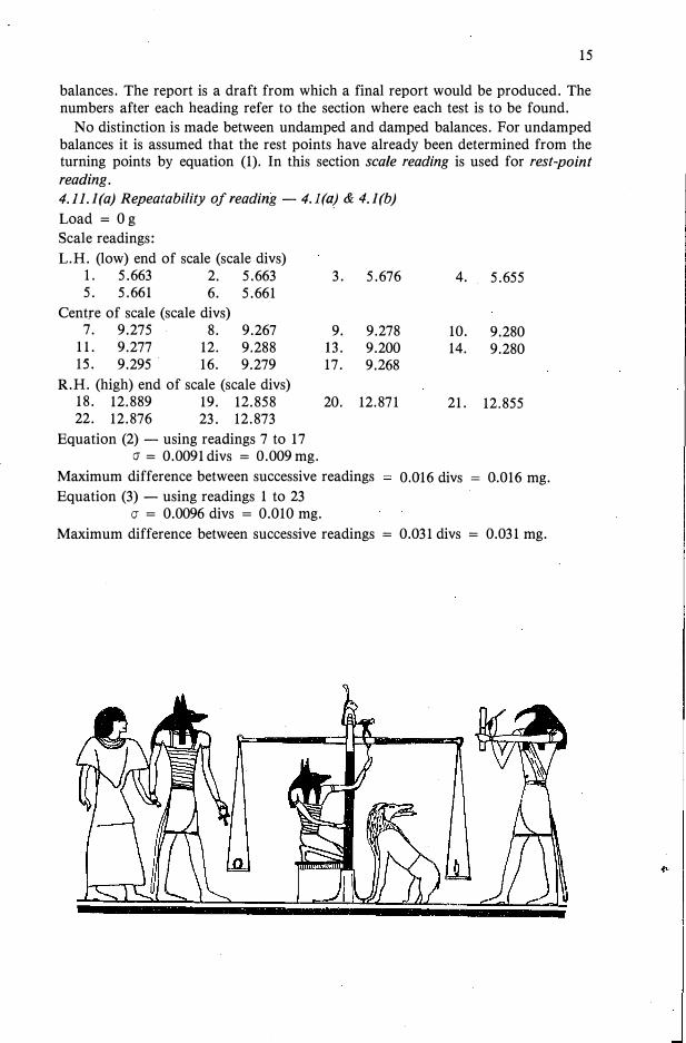
I

I I· :I I· I I

I' l

14

tilting of the stirrup about the knife will occur if the centre of mass of the suspension system (pan and stirrup) is not in the same vertical plane as the knife edge. This con­dition is characterised by a sharp rotation of the stirrup at the moment of release which sets the suspended system oscillating about the knife. This oscillation pro­duces a small periodic change in the reading on the scale.

The central knife should make contact with its plane last of all, so that the beam does not move before the end knives have made contact with their planes.

All these conditions can be rectified by using the adjusting screws in the arresting frame.

4.10 U$er Tests on Balances

With the almost total disappearance of two-pan balances from routine use there are now very few people who have had experience of servicing and adjusting them. This means that the user will often be thrown back onto his own resources, and he will have to learn the adjustments and tests described above. As most two-pan balances are used for mass calibration it becomes obvious immediately if something is wrong. For those balances which are used for normal weighing the following tests should be done every three to six months and then compared with previous results to ensure that the balance is still performing satisfactorily.

(a) Measure the repeatability of reading using one of the methods described in4.l(a) or 4.l(b). If the new value of the standard deviation is greater than 1.730 t( cr is the value of the standard deviation obtained previously) then the beam shouldbe removed and the knife-edges and planes carefully cleaned with alcohol ( or similarfluid that does not leave a film) and examined for damage with a micro�cope. Forthe knives this can be done by positioning lamps so that light is reflected from bothfacets into the microscope (NPL, 1954). A knife without defects should show a thindark line. If no damage is visible then they should be cleaned again and the balancereassembled, taking care that there is no dust on the knife-edges or planes.

(b) Measure the sensitivity-reciprocal for zero, half-maximum and maximumload. If it has changed by more than three times the standard deviation from the value previously obtained then the knife edges and planes should be cleaned as described in (a) and the arrestment checked.

(c) Check the ratio of arms as described in section 4.4. Any change in this value bymore than three times the standard deviation of the ratio of arms (see equation (6) and the calculation in section 4.11.4) indicates that either one of the knife edges has moved or some damage has occurred. The knife edges and planes should be examin­ed and if no damage has occurred the ratio of arms (and parallelism) re-adjusted. All the adjusting screws should be well tightened without causing damage.

It is very difficult to repair damaged knife edges or planes. The solution is preven­tion, i.e. great care in handling and use, as these balances are virtually irreplaceable.

4.11 Recording and Reporting of Results for Two-Pan Balances

Examples of the tests described in this chapter are given along with a sample report form. As only one example of each table is given not all numbers included in the report can be found in the tables. Most balances have only some of the features for which tests can be made and so some numbers are obtained from different

t F-test on 10 degrees of freedom at the 5% level.

'

,I

15

balances. The report is a draft from which a final report would be produced. The numbers after each heading refer to the section where each test is to be found.

No distinction is made between undamped and damped balances. For undamped balances it is assumed that the rest points have already been determined from the turning points by equation (1). In this section scale reading is used for rest-point reading. 4.11.l(a) Repeatability of reading - 4.J(a/ & 4.l(b) Load= Og Scale readings: L.H. (low) end of scale (scale divs)

1. 5.663 2. 5.663 3. 5.6765. 5.661 6. 5.661

Centre of scale (scale divs) 7. 9.275 8. 9.267 9. 9.278

11. 9.277 12. 9.288 13. 9.20015. 9.295 16. 9.279 17. 9.268

R.H. (high) end of scale (scale divs) 18. 12.889 19. 12.858 20. 12.87122. 12.876 23. 12.873

Equation (2) - using readings 7 to 17 a = 0.0091 divs = 0.009 mg.

4. 5.655

10. 9.28014. 9.280

21. 12.855

Maximum difference between successive readings Equation (3) - using readings 1 to 23

0.016 divs = 0.016 mg.

a = 0.0096 divs = 0.010 mg. Maximum difference between successive readings = 0.031 divs = 0.031 mg.

16

4.11.l(b) Repeatability of reading - 4.J(c)

Load = 200 g

Number Left Pan Right Pan Scale Reading h = (a- b)/2

1 M1 M2 a 1 = 10.691

M2 M1 b1 = 8.479 h, = 1.106

2 M1 M210.952 1.143

M2 M1

8.666

3 M1 M2

10.782 1.079M2

M1 8.624

4 M1 M2 10.558 1.005

I M2 M1

8.548! '

5 M1 M2

10.742 1.155M2

M1 8.433

6 M1 M2 10.626 1.006

M2 M1 8.615

7 M1 M2 10.610 1.083M2

M1 8.445

8 M1 M2 10.621 1.106M2 M1 8.410

9 M1 M2

10.717 1.119M2

M1 8.480

10 M1 M2 10.690 1.089M2 M1 8.512

CJ= 0.053 divs = 0.061 mg (equation (2))Maximum difference between successive readings = 0.150 divs = 0.173 mg

/i

i

,r

ji,'I

I\

4.11.2 Sensitivity - 4.2

Mass

ZeroPlus mass equal to full scale deflection = 0.006 68 gZeroSensitivity reciprocal (g/div)

Uncertainty:

Zero Load

Z 5.861m 12.453m 12.472Z 5.9110.001 015

Sensitivity reciprocal (SR) = mass/scale divs = m/h

(CJ,r)2 = ( �:) 2

(Jm2 + ( tr) 2

(Jh2

= CJ2;h2 + (m/h2)2 CJh212

m = 0.00668 g

Half Load200 g

8.52614.32214.3148.543

0.001 155

h = 6.58 divs (zero load) = 5.78 divs (half load)= 5.20 divs (full load)

(Jm = 0.000 0033 gCJh = 0.0096 (section 4.11.l(a))

17

Full Load500 g

8.11913.35313.348

8.1820.001 284

:. (CJsr)2 = 2.57 X 10-13 + 1.10 X 10-12 = 1.36 X lQ-12 (g/div) 2

For zero load, CJ,r = 1.17 x 10- 6 g/divUncertainty = 3 x 1.17 x 10-6

= 0.00 0035 g/div

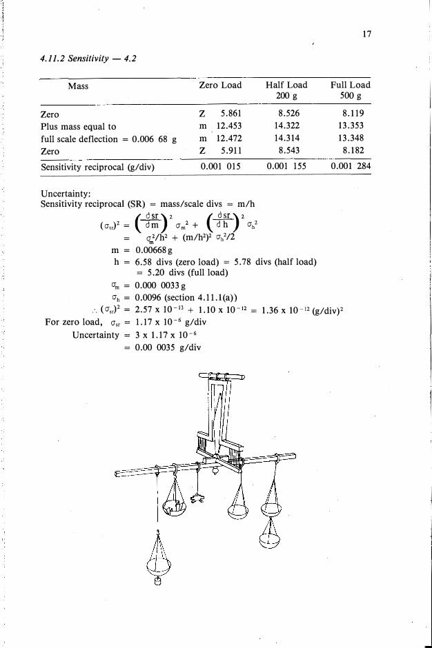
16

4.11.l(b) Repeatability of reading - 4.l(c)

Load = 200 g

Number Left Pan Right Pan Scale Reading h = (a- b)/2

1 M1 M2 a1 = 10.691

M2 M1 b1 ='

8.479 h1 = 1.106

2 M1 M2 10.952 1.143

M2 M1

8.666

3 M1 M2

10.782 1.079M2

M1 8.624

4 M1 M2

10.558 1.005M2 M1

8.548.

5 M1 M2 10.742 1.155

M2 M 1 8.433

6 M1 M2 10.626 1.006M2 M1 8.615

7 M1 M2

10.610 1.083M2 M1 8.445

8 M1 M2 10.621 1.106M2 M1 8.410

9 M1 M2 10.717 1.119M2 M 1

8.480

10 M1 M2 10.690 1.089M2 M1 8.512

(J = 0.053 divs = 0.061 mg (equation (2))Maximum difference between successive readings = 0.150 divs = 0.173 mg

4.11.2 Sensitivity - 4.2

Mass

Zero Plus mass equal to full scale deflection = 0.006 68 gZeroSensitivity reciprocal (g/div)

Uncertainty:

Zero Load

Z 5.861m 12.453m 12.472Z 5.9110.001 015

Sensitivity reciprocal (SR) = mass/scale divs = m/h

(cr,r)2 = ( ��)2

(Jm2 + ( tr) 2

(Jh2

= a 2/h2 + (m/h2)2 ah212

m = 0.00668 g

Half Load200 g

8.52614.32214.3148.543

0.001 155

h = 6.58 divs (zero load) = 5.78 divs (half load)= 5.20 divs (full load)

(Jm = 0.000 0033 g (Jh = 0.0096 (section 4.11.l(a))

17

Full Load500 g

8.11913.35313.348

8.1820.001 284

:. ((Jsr)2 = 2.57 X 10- 13 + 1.10 X 10- 12

= 1.36 X 10-12 (g/div)2

For zero load, a,r = 1.17 x 10- 6 g/divUncertainty = 3 x 1.17 x 10- 6

= 0.00 0035 g/div

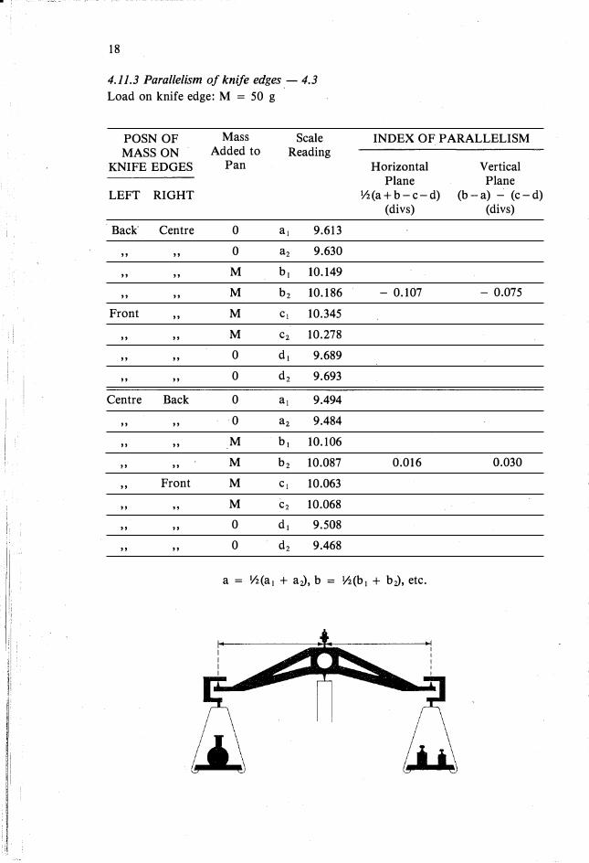
18

4.11.3 Parallelism of knife edges - 4.3

Load on knife edge: M = 50 g

POSN OF Mass Scale INDEX OF PARALLELISM MASS ON Added to Reading

KNIFE EDGES Pan Horizontal Vertical Plane Plane

LEFT RIGHT !h(a+b-c-d) (b - a) - (c -d) (divs) (divs)

Back Centre 0 a1 9.613

" " 0 a2 9.630

" " M b 1 10.149

" " M b2 10.186 - 0.107 - 0.075

Front " M C1 10.345

" " M Cz 10.278

" " 0 d 1 9.689

" " 0 d2 9.693

Centre Back 0 a1 9.494

" " 0 a2 9.484

,, " M b1 10.106

" " M b2 10.087 0.016 0.030

" Front M C1 10.063

" M C2 10.068

" ,, 0 d 1 9.508

" " 0 d2 9.468

a= V2(a 1 + az), b = Yi(b 1 + bz), etc.

,'

4.11.4 Ratio of arms - 4.4

Load M = 200 g Temperature 21 °C

Left Pan Right Pan

0 0 ro M1 M2 r1

M2 M 1 r2

M2 M1 r2

M 1 M2 r1

0 0 ro

The left arm is longer than the right by SR(r1 + r2 - 2r0)/2M

= [(0.756 X 0.001155)/400] X 106

= 2.2 ppm

Standard deviation of the ratio of arms

= 1.22 a /M.106 ppm

where a = 0.061 mg (section 4.11.l(b))

S d d d , t' 1.22 X 0.061 X 10- 3

106 tan ar evia 10n =

200

= 0.37 ppm

Scale Reading (divs)

9.308

8.545

10.755

10.723

8.561

9.227

19

Mean Values (divs)

r0 = 9.268 r1 = 8.553 r2 = 10.739

18

4.11.3 Parallelism of knife edges - 4.3

Load on knife edge: M = 50 g

POSN OF Mass Scale INDEX OF PARALLELISM MASS ON Added to Reading

KNIFE EDGES Pan Horizontal Vertical Plane Plane

LEFT RIGHT Yz(a+b-c-d) (b-a) - (c-d) (divs) (divs)

Back Centre 0 a 1 9.613

" ,, 0 a2 9.630

" " M b 1 10.149

" " M b2 10.186 - 0.107 - 0.075

Front ,, M C 1 10.345

" " M C2 10.278

,, " 0 d1 9.689

,, " 0 d2 9.693

Centre Back 0 a1 9.494

" " 0 a2 9.484

" " M b 1 10.106

" " M b2 10.087 0.016 0.030

,, Front M C1 10.063

" M C2 10.068

" ,, 0 d 1 9.508

,, ,, 0 d2 9.468

a = Yz(a 1 + az), b = Yz(b 1 + bz), etc.

4.11.4 Ratio of arms - 4.4

Load M = 200 g Temperature 21 °C

Left Pan Right Pan

0 0 ro

M1 M2 r1

M2 M1 r2

M2 M1 r2

M1 M2 r1

0 0 ro

The left arm is longer than the right by SR(r1 + r2 - 2r0)/2M

= [(0.756 X 0.001155)/400] X 106

= 2.2 ppm

Standard deviation of the ratio of arms = 1.22 u /M.106 ppm

where u = 0.061 mg (section 4.11.l(b))

S d d d , t' 1.22 X 0.061 X 10- 3

106

tan ar evia 10n =

200

= 0.37 ppm

Scale Reading (divs)

9.308

8.545

10.755

10.723

8.561

9.227

19

Mean Values (divs)

r0 = 9.268 r1 = 8.553 r2 = 10.739

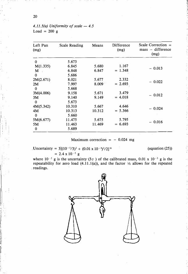
20 21

4.JJ.5(a) Uniformity of scale - 4.5 4.ll.5(b) Uniformity of scale - 4.5

Load = 200 g Load = 200 g Calibrating mass M = 1.000 mg Note: M' = M

Left Pan . Scale Reading Means Difference Scale Correction = (mg) (mg) mass - difference Left Scale Means Difference Scale Correction Cumulative

(mg) Pan Reading (mg) M - difference Correction

0 5.673 (mg) (mg)

M(l.335) 6.845 5.680 1.167 0 6.990

M 6.848 6.847 1.348 - 0.013 M 7.877 7.000 0.877 = - 0.013 - 0.0130 5.686 M 7.877 7.877 = 1.013

2M(2.671) 8.021 5.677 2.332 0 7.010 - 0.022

2M 7.997 8.009 = 2.693 M' 7.910 0 5.668 M' + M 8.872 8.000 0.874

3M(4.006) 9.158 5.671 3.479 - 0.012 M' + M 8.876 8.874 = 1.009 - 0.009 - 0.022

3M 9.140 9.149 = 4.018 M' 7.890 0 5.673

2M' 4M(5.342) 10.310 5.667 4.646 8.995

4M 10.313 10.312 = 5.366 - 0.024 2M' + M 9.855 9.000 0.857

0 5.660 2M' + M 9.859 9.857 = 0.990 + 0.010 - 0.012

5M(6.677) 11.475 5.675 5.795 2M' 9.005

5M 11.463 11.469 = 6.693 - 0.0163M' 10.007

0 5.689 3M' + M 10.872 10.000 0.876 3M' + M 10.880 10.876 = 1.012 - 0.012 - 0.024

Maximum correction = - 0.024 mg 3M' 9.993

.Uncertainty= 3.((10- 5/3)2 + (0.01 x lQ- 3)2/2] Y' 4M' 11.006

(equation (25)) 4M' + M 11.863 11.000 0.859 = 2.4 x 10- 5 g 4M' + M 11.855 11.859 = 0.992 + 0.008 - 0.016

where 10- 5 g is the uncertainty (30") of the calibrated mass, 0.01 x 10- 3 g is the 4M' 10.994 repeatability for zero load (4.11.l(a)), and the factor V2 allows for the repeated

Maximum correction = - 0.024 mg readings.

l1; ,1

20

4.11.5(a) Uniformity of scale - 4.5

Load = 200 g

Left Pan Scale Reading Means Difference Scale Correction =

(mg) (mg) mass - difference (mg)

0 5.673 M(l.335) 6.845 5.680 1.167

- 0.013M 6.848 6.847 1.348 0 5.686

2M(2.671) 8.021 5.677 2.332 - 0.022

2M 7.997 8.009 = 2.693 0 5.668

3M(4.006) 9.158 5.671 3.479 - 0.012

3M 9.140 9.149 = 4.018 0 5.673

4M(5.342) 10.310 5.667 4.646 - 0.024

4M 10.313 10.312 = 5.366 0 5.660

5M(6.677) 11.475 5.675 5.795 - 0.016

5M 11.463 11.469 = 6.693 0 5.689

Maximum correction = - 0.024 mg

.Uncertainty = 3't(I0- 5/3)2 + (0.01 x 10- 3) 2/2]"' (equation (25)) = 2.4 X lQ-5 g

where 10- 5 g is the uncertainty (3a ) of the calibrated mass, 0.01 x 10- 3 g is the repeatability for zero load (4.11. l(a)), and the factor Yz allows for the repeated readings.

.--

''{

21

4.11.5(b) Uniformity of scale - 4.5

Load = 200 g Calibrating mass M = 1.000 mg Note: M' ""' M

Left Scale Means Difference Scale Correction Cumulative Pan Reading (mg) M - difference Correction

(mg) (mg)

0 6.990 M 7.877 7.000 0.877 M 7.877 7.877 = 1.013 - 0.013 - 0.013

0 7.010

M' 7.910 M' + M 8.872 8.000 0.874 M' + M 8.876 8.874 = 1.009 - 0.009 - 0.022

M' 7.890

2M' 8.995 2M' + M 9.855 9.000 0.857 2M' + M 9.859 9.857 = 0.990 + 0.010 - 0.012

2M' 9.005

3M' 10.007 3M' + M 10.872 10.000 0.876 3M' + M 10.880 10.876 = 1.012 - 0.012 - 0.024

3M' 9.993

4M' 11.006 4M' + M 11.863 11.000 0.859 4M' + M 11.855 11.859 = 0.992 + 0.008 - 0.016

4M' 10.994

Maximum correction = - 0.024 mg

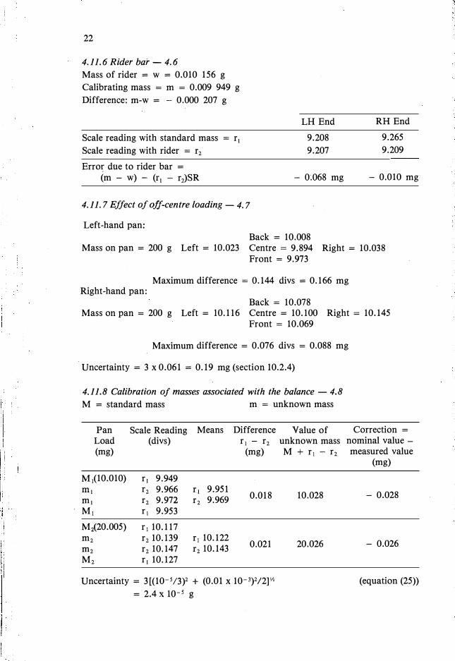
I �

i 1 ! ;! l

22

4.11.6 Rider bar - 4.6

Mass of rider = w = 0.010 156 g

Calibrating mass = m = 0.009 949 g

Difference: m-w = - 0.000 207 g

Scale reading with standard mass = r1

Scale reading with rider = r2

Erro� due to rider bar =

(m - w) - (r1 - r2)SR

4.11. 7 Effect of of !-centre loading - 4. 7

Left-hand pan:

LHEnd

9.208

9.207

- 0;068 mg

Back = 10.008

RH End

9.265

9.209

- 0.010 mg

Mass on pan = 200 g Left = 10.023 Centre = 9.894 Right = 10.038 Front = 9.973

Maximum difference = 0.144 divs = 0.166 mg Right-hand pan:

Back = 10.078 Mass on pan = 200 g Left = 10.116 Centre = 10.100 Right = 10.145

Front = 10.069

Maximum difference = 0.076 divs = 0.088 mg

Uncertainty = 3 x 0.061 = 0.19 mg (section 10.2.4)

4.11.8 Calibration of masses associated with the balance - 4.8

M = standard mass m = unknown mass

Pan Load (mg)

M 1(10.010) m 1

m 1

M 1

Mi{20.005) m2

m2 M2

Scale Reading (divs)

r 1 9.949 r2 9.966 r2 9.972 r1 9.953

r 1 10.117 r2 10.139 r2 10.147 r 1 10.127

Means Difference Value of

r 1 9.951 r2 9.969

r1 10.122 r2 10.143

r 1 - r2 unknown mass (mg) M + r 1 - r 2

0.018 10.028

0.021 20.026

Uncertainty = 3[(10-5/3)2 + (0.01 x 10-3)2f2]Yi

= 2.4 X 10-5 g

Correction =

nominal value -measured value

(mg)

- 0.028

- 0.026

(equation (25))

4.11.9 Sample Report on a three-knife-edge balance

REPORT ON TWO-PAN THREE-KNIFE-EDGE BALANCE

Maker Oertling Model - Serial No. 456 Capacity 500 g Scale Range 20. mg Scale Division 0.1 mg Reading to 0. OJ mg by means of optical readout Type of motion (damped or undamped) undamped Client CSIRO Examined at (precise location) Room C262, National Measurement Laboratory Temperature of test 20.2 °C

Repeatability of Reading

.23

This was determined for the loads and scale readings (inclination of the beam) as set out in the following table.

Load

zero

half maximum

maximum

Sensitivity

Scale Reading

Standard Deviation of reading (mg)

0.010

0.061

0.065

Maximum difference between successive readings (mg)

0.031

0.173

0.180

The sensitivity-reciprocal (i.e. the change in load required to change the rest-point by one small division) was determined over the full range of the scale for the loads given in the following table.

Load zero half maximum maximum 200 g 500 g

Sensitivity-reciprocal (mg/div) 1.015 1.155 1.284

Uncertainty (mg/div) 0.004 0.005 0.006

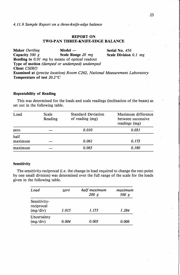
i 'I

!! I

'I ,I ll

,If j1

w

22

4.11.6 Rider bar - 4.6

Mass of rider = w = 0.010 156 g

Calibrating mass = m = 0.009 949 g

Difference: m-w = - 0.000 207 g

Scale reading with standard mass = r1

Scale reading with rider = r2

Error due to rider bar =

(m - w) - (r1 - r2)SR

4.11. 7 Effect of off-centre loading - 4. 7

Left-hand pan:

LHEnd

9.208

9.207

- 0;068 mg

Back = 10.008

RH End

9.265

9.209

- 0.010 mg

Mass on pan = 200 g Left = 10.023 Centre = 9.894 Right = 10.038

Front = 9.973

Maximum difference = 0.144 divs = 0.166 mg Right-hand pan:

Back = 10.078 Mass on pan = 200 g Left = 10.116 Centre = 10.100 Right = 10.145

Front = 10.069

Maximum difference = 0.076 divs = 0.088 mg

Uncertainty = 3 x 0.061 = 0.19 mg (section 10.2.4)

4.11.8 Calibration of masses associated with the balance - 4.8

M = standard mass m = unknown mass

Pan Load (mg)

M 1(10.010) m 1

m 1

M 1

Mz(20.005) m2

m2 M2

Scale Reading (divs)

f1 9.949 r2 9.966 r2 9.972 r 1 9.953

r 1 10.117 r2 10.139 r2 10.147 r 1 10.127

Means Difference r1 - r2

f 1 9.951 f2 9.969

r 1 10.122 f2 10.143

(mg)

0.018

0.021

Uncertainty = 3[(10- 5/3)2 + (0.01 x 10-3)2f2]Y'

= 2.4 X 10-5 g

Value of Correction = unknown mass nominal value -M + r 1 - r 2 measured value

(mg)

10.028 - 0.028

20.026 - 0.026

(equation (25))

4.11.9 Sample Report on a three-knife-edge balance

REPORT ON TWO-PAN THREE-KNIFE-EDGE BALANCE

Maker Oertling Model - Serial No. 456 Capacity 500 g Scale Range 20. mg Scale Division 0.1 mg Reading to 0. OJ mg by means of optical readout Type of motion (damped or undamped) undamped Client CS/RO Examined at (precise location) Room C262, National Measurement Laboratory Temperature of test 20.2 °C

Repeatability of Reading

.23

This was determined for the loads and scale readings (inclination of the beam) as set out in the following table.

Load

zero

half maximum

maximum

Sensitivity

Scale Reading

Standard Deviation of reading (mg)

0.010

0.061

0.065

Maximum difference between successive readings (mg)

0.031

0.173

0.180

The sensitivity-reciprocal (i.e. the change in load required to change the rest-point by one small division) was determined over the full range of the scale for the loads given in the following table.

Load zero half maximum maximum 200 g 500 g

Sensitivity-reciprocal (mg/div) 1.015 1.155 1.284

Uncertainty (mg/div) 0.004 0.005 0.006

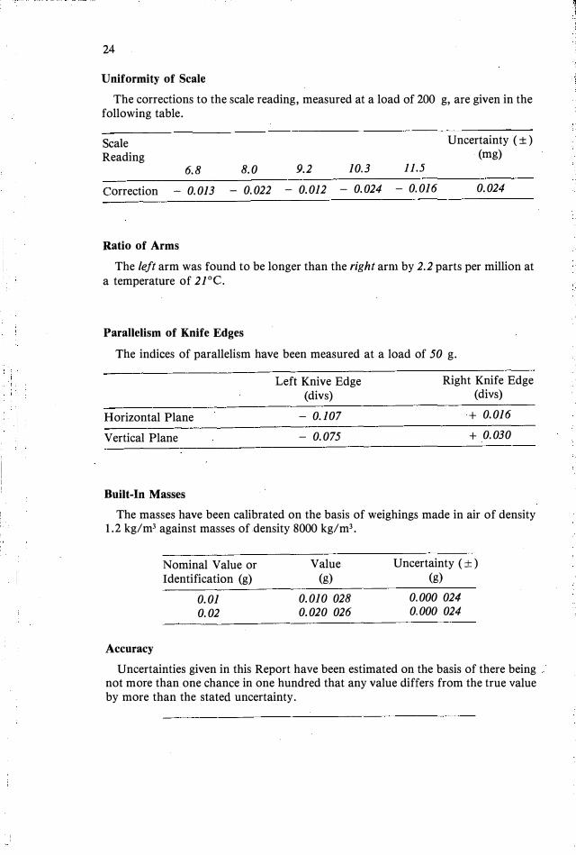
Cl

I I ! i ! !

24

Uniformity of Scale

The corrections to the scale reading, measured at a load of 200 g, are given in the following table.

Scale Uncertainty ( ±) Reading (mg)

6.8 8.0 9.2 10.3 11.5

Correction - 0.013 - 0.022 - 0.012 - 0.024 - 0.016 0.024

Ratio of Arms

The left arm was found to be longer than the right arm by 2.2 parts per million at a temperature of 21

°

c.

Parallelism of Knife Edges

The indices of parallelism have been measured at a load of 50 g.

Horizontal Plane

Vertical Plane

Built-In Masses

Left Knive Edge (divs)

- 0.107

- 0.075

Right Knife Edge (divs)

+ 0.016

+ 0.030

The masses have been calibrated on the basis of weighings made in air of density 1.2 kg/m3 against masses of .density 8000 kg/m3

•

Accuracy

Nominal Value or Identification (g)

0.01

0.02

Value (g)

0.010 028

0.020 026

Uncertainty ( ±) (g)

0.000 024

0.000 024

Uncertainties given in this Report have been estimated on the basis of there being not more than one chance in one hundred that any value differs from the true value by more than the stated uncertainty.

Notes

1. The balance has been tested according to the specifications laid down inThe Calibration of Balances

David B. Prowse CSIRO National Measurement Laboratory

Chapter 4 2. A reading consists of [delete (a), (b) or (c) as appropriate](a) releasing the balance without disturbing the load.

25

(b) removing the load behveen eaeh reading and using the differenee behveen thereading and zero in the calculations(c) interchanging masses on the pans and using half the difference between rest­points in the calculations.3. When the sign of the correction is positive ( +) the amount should be added to thescale reading to give the correct value and when negative ( - ) subtracted from it.

5. Calibration of Single-Pan, Two-Knife-Edge Balances

5.1 Repeatability of Reading

Repeatability is a measure of how well a balance will weigh. Ultimately all the other tests are to ensure that the correct mass value is obtained. The repeatability is normally expressed �n terms of the standard deviation obtained from a series of repeated readings together with the relative size of the maximum difference between two successive readings. For a good balance these should not exceed three times the discrimination. However the readings must be obtained in a way that realistically simulates how a balance is used in practice. Although these balances weigh at ap­proximately constant load, the repeatability should be measured with masses near half and maximum capacity of the balance and possibly both ends of the scale. This takes account of any variability due to positioning of the masses and also any effect due to the change in the centre of gravity of objects on the beam.

(a) The balance is released and the rest point, r 1 noted. This is repeated n times(n > 10) and the standard deviation calculated by means of the formula

r3 = [I(ri - f)2/(n-l)P" i

i = 1, ... ,n (7)

For a balance with a large scale range the procedure in section 4.1 (b) should be used. The value of the standard deviation obtained above gives the ultimate precision of

a balance. For analytical balances it should be measured occasionally as an indica­tion of the condition of the knife edges.

(b) A weighing consists of placing masses on and off the pan and (if appropriate)opening and closing the balance case. This causes a greater disturbance to the balance then merely releasing and arresting it. Also this may introduce some variability due to the positioning of the masses on the pans.

The most realistic way to assess the repeatability is to remove and replace the masses for each reading. Then the standard deviation should be calculated from the difference between the zero reading of the balance (zi) and the reading with a mass on the pan (mi), i.e. r i = m i - z i. Therefore

r3 = [ � (ri - f)2/(n -1)] v, i = l, ... ,n (8)

l,i ! I,

ij i,

:\1

,: 11 ,,

ii ;i

i. I

24

Uniformity of Scale

The corrections to the scale reading, measured at a load of 200 g, are given in the following table.

Scale Uncertainty ( ±) Reading (mg)

6.8 8.0 9.2 10.3 11.5

Correction - 0.013 - 0.022 - 0.012 - 0.024 - 0.016 0.024

Ratio of Arms

The left arm was found to be longer than the right arm by 2.2 parts per million at a temperature of 21°C.

Parallelism of Knife Edges

The indices of parallelism have been measured at a load of 50 g.

Horizontal Plane

Vertical Plane

Built-In Masses

Left Knive Edge (divs)

0.107

0.075

Right Knife Edge (divs)

+ 0.016

+ 0.030

The masses have been calibrated on the basis of weighings made in air of density 1.2 kg/m3 against masses of density 8000 kg/m3

•

Accuracy

Nominal Value or Identification (g)

0.01 0.02

Value (g)

0.010 028 0.020 026

Uncertainty ( ±) (g)

0.000 024 0.000 024

Uncertainties given in this Report have been estimated on the basis of there being not more than one chance in one hundred that any value differs from the true value by more than the stated uncertainty.

i

Notes

1. The balance has been tested according to the specifications laid down inThe Calibration of Balances

David B. Prowse CSIRO National Measurement Laboratory

Chapter 4 2. A reading consists of [delete (a), (b) or (c) as appropriate](a) releasing the balance without disturbing the load.

25

(b) removing the load between each reading and using the difference behveen thereading and z@ro in th@ cakulations(c) interchanging masses on the pans and using half the difference between rest­points in the calculations.3. When the sign of the correction is positive ( +) the amount should be added to thescale reading to give the correct value and when negative ( - ) subtracted from it.

5. Calibration of Single-Pan, Two-Knife-Edge Balances

5.1 Repeatability of Reading

Repeatability is a measure of how well a balance will weigh. Ultimately all the other tests are to ensure that the correct mass value is obtained. The repeatability is normally expressed �n terms of the standard deviation obtained from a series of repeated readings together with the relative size of the maximum difference between two successive readings. For a good balance these should not exceed three times the discrimination. However the readings must be obtained in a way that realistically simulates how a balance is used in practice. Although these balances weigh at ap­proximately constant load, the repeatability should be measured with masses near half and maximum capacity of the balance and possibly both ends of the scale. This takes account of any variability due to positioning of the masses and also any effect due to the change in the centre of gravity of objects on the beam.

(a) The balance is released and the rest point, r 1 noted. This is repeated n times(n > 10) and the standard deviation calculated by means of the formula

CJ = [ I(ri - f)2/(n- l)P' i = l, ... ,n (7) i

For a balance with a large scale range the procedure in section 4.1 (b) should be used. The value of the standard deviation obtained above gives the ultimate precision of

a balance. For analytical balances it should be measured occasionally as an indica­tion of the condition of the knife edges.

(b) A weighing consists of placing masses on and off the pan and (if appropriate)opening and closing the balance case. This causes a greater disturbance to the

. balance then merely releasing and arresting it. Also this may introduce some variability due to the positioning of the masses on the pans.

The most realistic way to assess the repeatability is to remove and replace the masses for each reading. Then the standard deviation should be calculated from the difference between the zero reading of the balance (zt) and the reading with a mass on the pan (mt), i.e. r i = mi - z j. Therefore

CJ= [ �(ri - f)2/(n- l)]Yz i = 1, ... ,n (8)

,,

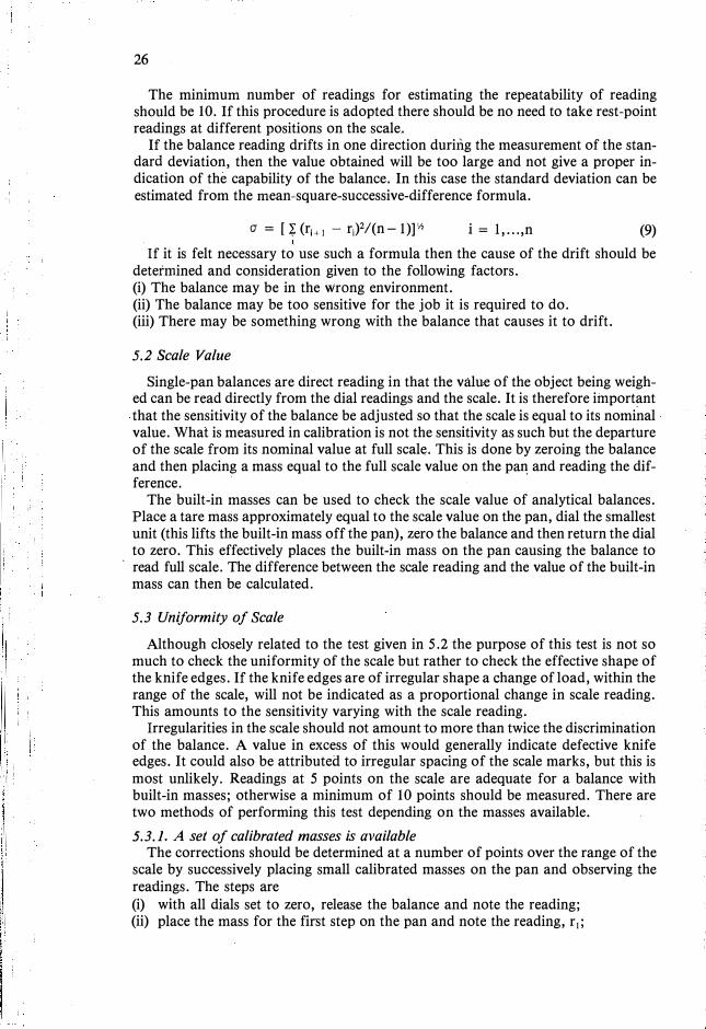
I

1 ! I

II,

26

The minimum number of readings for estimating the repeatability of reading should be 10. If this procedure is adopted there should be no need to take rest-point readings at different positions on the scale.

If the balance reading drifts in one direction during the measurement of the stan­dard deviation, then the value obtained will be too large and not give a proper in­dication of the capability of the balance. In this case the standard deviation can be estimated from the mean-square-successive-difference formula.

a = [ � (r;+i - r;)2/(n- l)]Y, i = l, ... ,n (9)

If it is felt necessary to use such a formula then the cause of the drift should be determined and consideration given to the following factors. (i) The balance may be in the wrong environment.(ii) The balance may be too sensitive for the job it is required to do.(iii) There may be something wrong with the balance that causes it to drift.

5.2 Scale Value

Single-pan balances are direct reading in that the value of the object being weigh­ed can be read directly from the dial readings and the scale. It is therefore important that the sensitivity of the balance be adjusted so that the scale is equal to its nominal value. What is measured in calibration is not the sensitivity as such but the departure of the scale from its nominal value at full scale. This is done by zeroing the balance and then placing a mass equal to the full scale value on the pan and reading the dif­ference.

The built-in masses can be used to check the scale value of analytical balances. Place a tare mass approximately equal to the scale value on the pan, dial the smallest unit (this lifts the built-in mass off the pan), zero the balance and then return the dial to zero. This effectively places the built-in mass on the pan causing the balance to

· read full scale. The difference between the scale reading and the value of the built-inmass can then be calculated.

5.3 Uniformity of Scale

Although closely related to the test given in 5.2 the purpose of this test is not so much to check the uniformity of the scale but rather to check the effective shape of the knife edges. If the knife edges are of irregular shape a change of load, within the range of the scale, will not be indicated as a proportional change in scale reading. This amounts to the sensitivity varying with the scale reading.

Irregularities in the scale should not amount to more than twice the discrimination of the balance. A value in excess of this would generally indicate defective knife edges. It could also be attributed to irregular spacing of the scale marks, but this is most unlikely. Readings at 5 points on the scale are adequate for a balance with built-in masses; otherwise a minimum of 10 points should be measured. There are two methods of performing this test depending on the masses available.

5.3.1. A set of calibrated masses is available The corrections should be determined at a number of points over the range of the

scale by successively placing small calibrated masses on the pan and observing the readings. The steps are (i) with all dials set to zero, release the balance and note the reading;(ii) place the mass for the first step on the pan and note the reading, r1;

27

(iii) re-read the zero - this reading is averaged with the reading in (i) to give the zeroreading for the calculation, z1 ;

(iv) repeat steps (ii) and (iii) to cover the whole scale.If M; is the value of the calibrated mass placed on the pan then the correction to

the scale reading at each point is given by

C1 = M; - (r; - z;).

The correction is the amount that should. be added to the scale reading to give the correct mass when a reading is made at that point of the scale.

The above method requires calibrated masses with an uncertainty less than the discrimination of the balance. Otherwise apparent non-uniformity may be due to the masses. 5.3.2 A set of calibrated masses is not available

In this case the scale is tested at equal increments with only one calibrating mass M, which should be no more than one-fifth of the range. The method is as follows: (i) read the balance zero;(ii) place the mass M on the pan and note the reading, r 1; (iii) re-read the zero, this reading is averaged with the reading in (i) to give the zero

value used in the calculation, z 1;

(iv) tare masses are added to the pan until the balance reading is close or equal to r i,note the reading;

(v) with the tare masses still on the pan, add the calibrating mass and note thereading, r2:

(vi) remove the calibrating mass and re-read, the average of this value with thatgiven in (iv) is denoted z2, (Note: the numerical value of z2 etc. will not be closeto zero);

(vii)repeat steps (iv) to (vi) to cover the whole scale.The corrections are calculated by:

C 1 = M - (r 1 - z 1)

C2 = M - (r2 - zz) etc.,

where C1, C2, etc. are the corrections for each scale interval. For these to be equivalent to the corrections in 5.3.1 the cumulative corrections must be calculated, i.e. C1, C1 + C2, C1 + C2 + C3 , etc. This method does not require any calibratedmasses other than M, and although by its nature is more time consuming than themethod of 5.3.1 it often provides more consistent values.

If the value of M is not known accurately then this method gives the non-linearity of the scale. However the corrections will depart from their true value by a fixed but unknown amount and cannot be used to correct the reading on the balance. If M is an integer fraction of the range (i.e. M = r 1 - z i, giving C 1 = 0), then the total cumulative correction can be equated to the scale value at full scale (section 5 .2), and numerically accurate corrections obtained over the full scale by the following calculation:

correction (i) "" iM(S + Kr)/R - K,

where R is the range of the balance scale (i.e. full scale), Kr is the calculated cumulative correction at full scale, Ki = C 1 + C2 + .... + C1, S "" measured correction to the scale value (section 5.2), i "" 1, 2, ... numerical order of calibrating the scale.

(10)

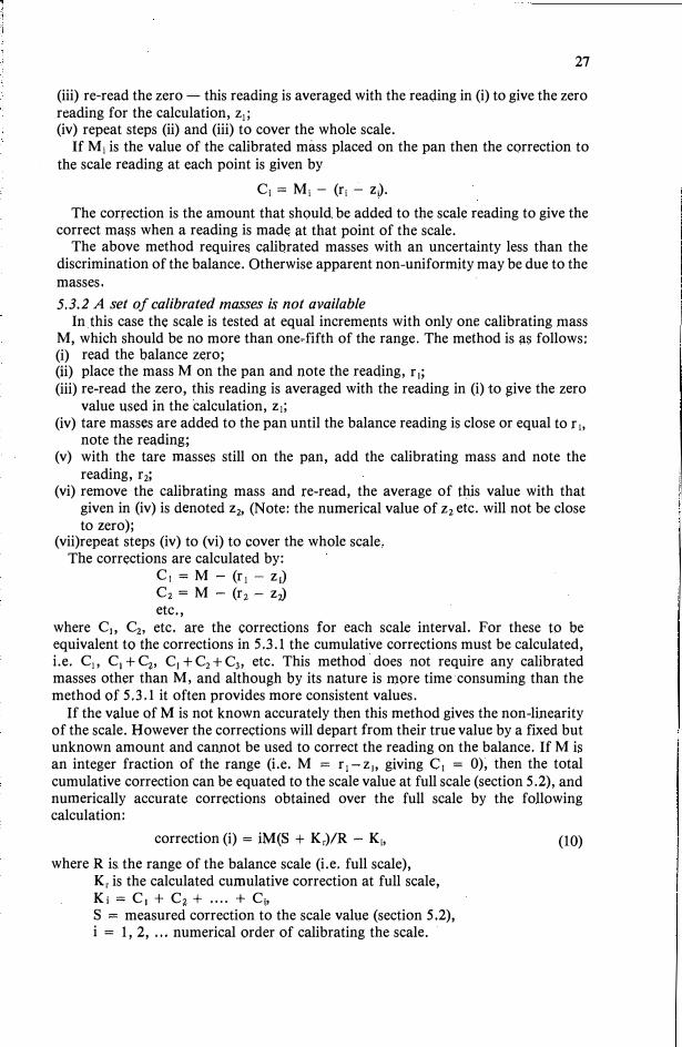
26

The minimum number of readings for estimating the repeatability of reading should be 10. If this procedure is adopted there should be no need to take rest-point readings at different positions on the scale.

If the balance reading drifts in one direction during the measurement of the stan­dard deviation, then the value obtained will be too large and not give a proper in­dication of the capability of the balance. In this case the standard deviation can be estimated from the mean-square-successive-difference formula.

a = [ 4 (ri+t - r)2/(n- l)]v, i = 1, ... ,n (9)

If it is felt necessary to use such a formula then the cause of the drift should be determined and consideration given to the following factors. (i) The balance may be in the wrong environment.(ii) The balance may be too sensitive for the job it is required to do.(iii) There may be something wrong with the balance that causes it to drift.

5.2 Scale Value

Single-pan balances are direct reading in that the value of the object being weigh­ed can be read directly from the dial readings and the scale. It is therefore important that the sensitivity of the balance be adjusted so that the scale is equal to its nominal value. What is measured in calibration is not the sensitivity as such but the departure of the scale from its nominal value at full scale. This is done by zeroing the balance and then placing a mass equal to the full scale value on the pan and reading the dif­ference.

The built-in masses can be used to check the scale value of analytical balances. Place a tare mass approximately equal to the scale value on the pan, dial the smallest unit (this lifts the built-in mass off the pan), zero the balance and then return the dial to zero. This effectively places the built-in mass on the pan causing the balance to read full scale. The difference between the scale reading and the value of the built-in mass can then be calculated.

5.3 Uniformity of Scale

Although closely related to the test given in 5.2 the purpose of this test is not so much to check the uniformity of the scale but rather to check the effective shape of the knife edges. If the knife edges are of irregular shape a change of load, within the range of the scale, will not be indicated as a proportional change in scale reading. This amounts to the sensitivity varying with the scale reading.

Irregularities in the scale should not amount to more than twice the discrimination of the balance. A value in excess of this would generally indicate defective knife edges. It could also be attributed to irregular spacing of the scale marks, but this is most unlikely. Readings at 5 points on the scale are adequate for a balance with built-in masses; otherwise a minimum of 10 points should be measured. There are two methods of performing this test depending on the masses available.

5.3.1. A set of calibrated masses is available The corrections should be determined at a number of points over the range of the

scale by successively placing small calibrated masses on the pan and observing the readings. The steps are (i) with all dials set to zero, release the balance and note the reading;(ii) place the mass for the first step on the pan and note the reading, r1;

27

(iii) re-read the zero � this reading is averaged with the reading in (i) to give the zeroreading for the calculation, z

1;

(iv) repeat steps (ii) and (iii) to cover the whole scale.If Mi is the value of the calibrated mass placed on the pan then the correction to

the scale reading at each point is given by

C1 = Mi - (ri - z;).

The correction is the amount that should. be added to the scale reading to give the correct mass when a reading is made at that point of the scale.

The above method requires calibrated masses with an uncertainty less than the discrimination of the balance. Otherwise apparent non-uniformity may be due to the masses. 5.3.2 A set of calibrated masses is not available

In. this case the scale is tested at equal increments with only one calibrating mass M, which should be no more than one-fifth of the range. The method is as follows: (i) read the balance zero;(ii) place the mass M on the pan and note the reading, r 1 ;

(iii) re-read the zero, this reading is averaged with the reading in (i) to give the zerovalue used in the calculation, z 1 ;

(iv) tare masses are added to the pan until the balance reading is close or equal to r i, note the reading;

(v) with the tare masses still on the pan, add the calibrating mass and note thereading, r2;

(vi) remove the calibrating mass and re-read, the average of this value with thatgiven in (iv) is denoted z2, (Note: the numerical value of z2 etc. will not be closeto zero);

(vii)repeat steps (iv) to (vi) to cover the whole scale.The corrections are calculated by:

C, = M - (r 1 - z 1) C2 = M - (r2 - zz) etc.,

where C,, C2, etc. are the corrections for each scale interval. For these to be �quivalent to the corrections in 5.3.1 the cumulative corrections must be calculated,1.e. Ci, C, + C2, C1 + C2 + C3 , etc. This method does not require any calibratedmasses other than M, and although by its nature is more time consuming than themethod of 5.3.1 it often provides more consistent values.

If the value of M is not known accurately then this method gives the non-linearity of the scale. However the corrections will depart from their true value by a fixed but unknown amount and cannot be used to correct the reading on the balance. If M is an integer fraction of the range (i.e. M = r 1 -z 1, giving C, = 0), then the total cumulative correction can be equated to the scale value at full scale (section 5.2), and numerically accurate corrections obtained over the full scale by the following calculation:

correction (i) "" iM(S + K r)/R - Ki,

where R is the range of the balance scale (i.e. full scale), K r is the calculated cumulative correction at full scale, Ki = C 1 + C2 + .... + Ci, S = measured correction to the scale value (section 5 .2), i = 1, 2, ... numerical order of calibrating the scale.

(10)

28

5.3.3 Interpolating between scale divisions Some analytical balances have a digital readout to interpolate between the scale

divisions. The uniformity and calibration of this scale can be measured exactly as for the optical scale, provided masses ofthe correct value are avai�able. How�v��, each end of the digital readout should coincide exactly with an optical scale d1V1s10n: If

this is not the case the balance should be returned for repair. The method of sect10n 5.3.2 can be used to measure the value at half range of the digital �c�le. If �n optical scale division is 1 mg or less, then small masses made from alummmm foil and ad­justed on the balance itself can be used.

5.4 Effect of Off-Centre Loading

When the centre of mass of the object being weighed is off-centre on the pan, shift or corner-load error may occur. It is difficult to produce figures that can be used to correct the balance readings because the effect is not always linear with respect to either load or position. This test is designed to enable the user to deci�e. how a�­curately objects must be positioned on the pan for this effect to be neghg1ble. It 1s particularly important for top-loading balances, but it can also affect the perfor­mance of analytical balances.

This effect is most easily measured by placing a mass on the centre of the pan and then moving it successively to the front, rear, left and ri�ht position� on th� pan, noting the reading each time. Accurate masses are not reqmred, any smtable piece of turned brass or stainless steel being adequate.

Readings at both ends of the scale are used in the adjustment of top-loadin_gbalances and so for both these and balances with only one decade, where the scale 1s long, this effect should be measured at both ends of the scale. If single, or stackable, masses are not available for this test, then appropriate small masses can be placed on a suitable part of the pan to bring the reading to full scale.

Problems arise as to (i) the magnitude of the mass placed on the pan, (ii) the shape of the mass, and (iii} how far the mass should be moved. (i) Most balance manufacturers recommend that the effect be measured at approxi­mately one-third or one-half the maximum load of the balance, or they quote per­formance figures at this load. Because this effect is often non-linear, measurementat a larger load will not necessarily give a larger reading. Also placing. a large ma�snear the edge of the pan could possibly do some damage to the mechamsm. Hence it is recommended that the test be carried out at the load recommended by the manufacturer, or, if this is not known, then it should be approximately one-third the maximum capacity of the balance. It is stressed that a single mass should be used f_orthis test and this restricts the choice to values of 1, 2, 5 and perhaps 3 (unless special masses ;hat can be stacked are available). For example, a balance of 1200 g capacity should be tested with a 500 g mass, because 200 g is too small. (ii) Masses from different manufacturers differ in shape so that when their edgesare aligned with the edge of the pan the centres of mass will be different distancesfrom the pan centre. For balances up to 10 kg capacity this p�oble� can be over­come if a disc of light material (aluminium, perspex, etc.) of d1mens10ns 10 ?1-m by 50 mm diameter is placed on the pan and the mass placed on top. The disc can always be moved the same distance regardless of the shape of the mass. F_oranalytical balances, and those with a pan diameter less than 100 mm, a 20 mm disc

.---

29

of conducting material (to eliminate the effects of static electricity) should be used. A disc need not be used for balances of capacity greater than 10 kg. (iii) The observed error depends crucially upon how far the mass is moved. Balancemanufacturers move the mass to the lip of the pan, defined as that area where theflat surface of the pan starts to curve up. This is considered the best position. Somebalances have a flat pan with a small 'ridge' at the edge. In this case it is possible forthe mass on the disc to overhang the edge of the pan during the test. This is unlikelyto be serious provided the test mass is no more than one-third of the capacity, andshould not affect the values obtained. For those analytical balances which have pansthat are portions of a sphere without a lip, the disc should be moved until its edgejust touches the edge of the pan, or the pan support. Care should be taken that thepan does not touch the case.

Some users change or modify their pans. In these cases an attempt should be made to carry out and report the test in a logical way.

5.5 Effect of Tare

Most single-pan balances have a taring facility which enables the balance to be zeroed with an applied load, usually up to the capacity of the balance. The tare device often consists of a spring which can be tensioned by the turning of a knob. The sensitivity may change with load if the tare spring is not correctly positioned.

Any errors in the tare system can be determined by placing a mass on the pan and using the tare to zero the scale. The mass used to test the full-scale value in section 5.2 is then placed on the pan and the reading on the scale compared with that given in 5.2. If the values differ by more than twice the standard deviation (section 5.l(b)), then the tare mechanism should be adjusted.

It is difficult to apply corrections for any error in the tare because the tare in­dicator is usually not graduated. If it is necessary to do precision weighing on a balance with such an error, then the scale value should be meas.ured for each tare set­ting used.

5. 6 Hysteresis

In a mechanical system hysteresis is almost always caused by friction. Two-panand analytical single-pan balances usually show no detectable hysteresis. Top­loading balances have more components that can be affected by friction, but a prop­erly adjusted balance in good condition should show no more hysteresis than 0.1 scale division. A balance showing more hysteresis than this needs either adjusting or cleaning. It is only necessary to test for hysteresis a few times during the life of the balance.

A test at one point, about mid-scale, is adequate. Proceed as follows: (i) zero the balance, z1 ;

(ii) place a mass M, equal to half the scale, on the pan, m1 ;

(iii) add extra mass to bring the balance reading close to full scale;(iv) remove the extra mass and read the balance with M still on the pan, m2;

(v) remove M and read the zero, z2 •

Repeat the above procedure three times and average the differences (m1-m2) and (z1-z2), which are a measure of the hysteresis of the balance.

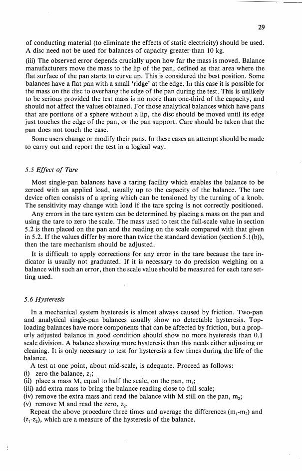
i I

Ii

i .i

28

5.3.3 Interpolating between scale divisions Some analytical balances have a digital readout to interpolate between the scale

divisions. The uniformity and calibration of this scale can be measured exactly as for the optical scale, provided masses of.the correct value are available. How�v��, each end of the digital readout should coincide exactly with an optical scale d1V1sion: If

this is not the case the balance should be returned for repair. The method of sect10n 5.3.2 can be used to measure the value at half range of the digital scale. If an optical scale division is 1 mg or less, then small masses made from aluminium foil and ad­justed on the balance itself can be used.

5.4 Effect of Off-Centre Loading

When the centre of mass of the object being weighed is off-centre on the pan, shift or corner-load error may occur. It is difficult to produce figures that can be used to correct the balance readings because the effect is not always linear with respect to either load or position. This test is designed to enable the user to deci�e. how a�­curately objects must be positioned on the pan for this effect to be neghgible. It is particularly important for top-loading balances, but it can also affect the perfor­mance of analytical balances.

This effect is most easily measured by placing a mass on the centre of the pan and then moving it successively to the front, rear, left and right positions on the pan, noting the reading each time. Accurate masses are not required, any suitable piece of turned brass or stainless steel being adequate.

Readings at both ends of the scale are used in the adjustment of top-loadin.gbalances and so for both these and balances with only one decade, where the scale is long, this effect should be measured at both ends of the scale . If single, or stackable, masses are not-available for this test, then appropriate small masses can be placed on a suitable part of the pan to bring the reading to full scale.

Problems arise as to (i) the magnitude of the mass placed on the pan, (ii) the shape of the mass, and (iii) how far the mass should be moved. (i) Most balance manufacturers recommend that the effect be measured at approxi­mately one-third or one-half the maximum load of the balance, or they quote per­formance figures at this load. Because this effect is often non-linear, measurementat a larger load will not necessarily give a larger reading. Also placing. a large ma�snear the edge of the pan could possibly do some damage to the mechamsm. Hence it is recommended that the test be carried out at the load recommended by the manufacturer, or, if this is not known, then it should be approximately one-third the maximum capacity of the balance. It is stressed that a single mass should be used f.or this test and this restricts the choice to values of 1, 2, 5 and perhaps 3 (unless special masses ;hat can be stacked are available). For example, a balance of 1200 g capacity should be tested with a 500 g mass, because 200 g is too small. (ii) Masses from different manufacturers differ in shape s.o that .when the�r edgesare aligned with the edge of the pan the centres of mass will be different distances from the pan centre. For balances up to 10 kg capacity this problem can be over­come if a disc of light material (aluminium, perspex, etc. ) of dimensions 10 �m by 50 mm diameter is placed on the pan and the mass placed on top. The disc can always be moved the same distance regardless of the shape of the mass. F.or analytical balances, and those with a pan diameter less than 100 mm, a 20 mm disc

29

of conducting material (to eliminate the effects of static electricity) should be used. A disc need not be used for balances of capacity greater than 10 kg. (iii) The observed error depends crucially upon how far the mass is moved. Balancemanufacturers move the mass to the lip of the pan, defined as that area where theflat surface of the pan starts to curve up. This is considered the best position. Somebalances have a flat pan with a small 'ridge' at the edge. In this case it is possible forthe mass on the disc to overhang the edge of the pan during the test. This is unlikelyto be serious provided the test mass is no more than one-third of the capacity, andshould not affect the values obtained. For those analytical balances which have pansthat are portions of a sphere without a lip, the disc should be moved until its edgejust touches the edge of the pan, or the pan support. Care should be taken that thepan does not touch the case.

Some users change or modify their pans. In these cases an attempt should be made to carry out and report the test in a logical way.

5.5 Effect of Tare

Most single-pan balances have a taring facility which enables the balance to be zeroed with an applied load, usually up to the capacity of the balance. The tare device often consists of a spring which can be tensioned by the turning of a knob. The sensitivity may change with load if the tare spring is not correctly positioned.

Any errors in the tare system can be determined by placing a mass on the pan and using the tare to zero the scale. The mass used to test the full-scale value in section 5. 2 is then placed on the pan and the reading on the scale compared with that givenin 5.2. If the values differ by more than twice the standard deviation (section 5.l(b)),then the tare mechanism should be adjusted.

It is difficult to apply corrections for any error in the tare because the tare in­dicator is usually not graduated. If it is necessary to do precision weighing on a balance with such an error, then the scale value should be meas.ured for each tare set­ting used.

5. 6 Hysteresis

In a mechanical system hysteresis is almost always caused by friction. Two-panand analytical single-pan balances usually show no detectable hysteresis. Top­loading balances have more components that can be affected by friction, but a prop­erly adjusted balance in good condition should show no more hysteresis than 0.1 scale division. A balance showing more hysteresis than this needs either adjusting or cleaning. It is only necessary to test for hysteresis a few times during the life of the balance.

A test at one point, about mid-scale, is adequate. Proceed as follows: (i) zero the balance, z1 ;

(ii) place a mass M, equal to half the scale, on the pan, m1 ;

(iii) add extra mass to bring the balance reading close to full scale;(iv) remove the extra mass and read the balance with M still on the pan, m2 ;

(v) remove M and read the zero, z2 •

Repeat the above procedure three times and average the differences (m1-m2) and(z 1-z2), which are a measure of the hysteresis of the balance.

i I

I !

30

5. 7 Miscellaneous5. 7.1 Level indicator

If the level of a balance is changed, different parts of the knife-edges, etc. are used

and the readings may be different. It is therefore important before calibration or use

to carefully level the balance, as determined by the attached level indicator. In some

cases the levelindicator may not be sufficiently sensitive. This can be tested by tilting

the balance, alternately in each direction, until the edge of the bubble just touches

the circle (most level indicators on balances are of the bulls-eye type). The balance

should then be zeroed and the scale value measured. If this value differs from that

given in section 5.2 by more than 2a [equation (7) or (8)], the level indicator is prob­

ably not sufficiently sensitive. This means that if the balance is moved at all then the

scale value should be remeasured. As a general rule the scale value should be remeasured whenever a balance is mov-

ed from the bench on which it is calibrated.

5.7.2 Drift Temperature gradients cause readings on all balances to change. Some balances,

particularly micro or semi-micro balances, are more susceptible than others to this drift in the reading. This is particularly noticeable when an operator sits in front of them. The significance of this effect can be assessed by noting the reading every two or three minutes until three successive readings do not change by more than the stan­dard deviation (section 5.1). Obviously the standard deviation must have been measured when the balance was free from drift, or the drift allowed for as described in section 5 .1.

If the balance reading is changing uniformly (the usual situation, at least to a first approximation) and the readings are made at equal time intervals, then moderate drift may be easily eliminated. For example, if readings are made in the following order

zero reading - z1

reading - m1

reading - m2

zero reading - z2,

then drift is eliminated if the mass of the object being weighed is calculated by the following formula

(11)

For precision weighing equation (11), or a similar equation, should always be us­ed. 5. 7.3 Balance arrestment

Analytical balances have an arrestment mechanism for the beam and the panknife edge. These balances are subject to the same problems, such as 'heel-and toe­ing', as three-knife-edge balances. The problems and their remedies as discussed in section 4.9, are equally applicable to two-knife edge balances, although the ad­justing screws are usually not as accessible.

5.8 Masses Installed in the Balance

Nearly all single-pan balances have masses installed in the balance. These masses are commonly referred to as built-in (or in-built) masses. Some balances have three or even four decades of masses and a full calibration can be very time consuming.

31

There are a number of possible methods of performing a calibration and these are described in the following sections. This should be the last test performed on the balance and it requires a set of masses which have an uncertainty not greater than the standard deviation of the balance.

Note that when calibrating a balance with built-in masses it is very important to distinguish between the value indicated by the balance (or the value of the built-in masses), and the reading obtained when a standard mass is placed on the pan. An example will help make this clear.

Consider a dial setting of 20 g. During calibration, a 20 g standard is placed on the pan and the balance reads 20.01 g. If a standard of mass 19.99 g were placed on the pan the balance would read 20.00 g. Therefore the true value associated with the 20 g dial setting is 19.99 g, not 20.01 g. In other words, the balance has a correction of -0.01 g at 20 g. The actual value of the built-in mass (or masses) is also 19.99 g. This .is apparent because placing 19.99 g on the pan and lifting the '20 g' built-in mass off the pan leaves the reading unchanged.

In reporting the result of the calibration of the built-in masses it is important to give the mass value for the dial setting, or the corresponding correctior,. Here

correction = value of the standard - balance reading = 20.00 - 20.01 = -0.01 g.

In either case the user has merely to add up the true values for the dial settings us­ed to obtain the correct mass of the object being weighed. In the above example the reading of 20.01 g should not be given in the Report as this will almost certainly result in the wrong value being used in calculating the mass.

When more than one dial setting is used, the usual case in practice, the correc­tions, or mass values, for each dial reading are added together to give the total cor­rection or value. 5.8.1 Removing the masses from the balance

In general this is not possible without almost completely dismantling the balance and risking scratching the masses as they are removed from or replaced in the balance. The balance mechanism and the masses are a unity and if the masses are calibrated in situ, then any small errors that may occur from the mechanism are ef­fectively calibrated out of the system. 5.8.2 Calibration of each dial setting by direct calibration

This involves measuring the correction for each dial setting by using appropriate masses from a calibrated set. The method is described by the following steps: (i) with all dials set to zero and no load on the pan, release the balance and note thereading, z 1 ;

(ii) set the "l" on the dial to be tested, place a calibrated mass of equivalent valueon the pan, release the balance and note the reading, m1 ;

(iii) repeat step (ii), either just releasing the balance, or preferably, removing themass and replacing it, m2;

(iv) return the dial to zero, remove the mass from the pan and read the zero, z2, thisbecomes the first zero reading for the next dial setting to be calibrated;(v) repeat steps (ii) to (iv) for all the dial settings of the balance.

The correction C to the dial setting is calculated by means of the following for­mula:

C = M - [(m1 + m2)/2 - (z1 + z2)/2],

where M is the value of the calibrating mass.

(12)

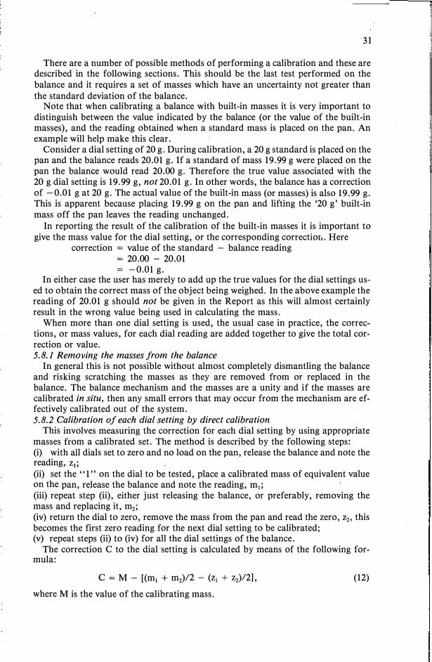
ii

ii !i

II

30

5. 7 Miscellaneous5. 7.1 Level indicator

If the level of a balance is changed, different parts of the knife-edges, etc. are used

and the readings may be different. It is therefore important before calibration or use

to carefully level the balance, as determined by the attached level indicator. In some

cases the levelindicator may not be sufficiently sensitive. This can be tested by tilting

the balance, alternately in each direction, until the edge of the bubble just touches

the circle (most level indicators on balances are of the bulls-eye type). The balance

should then be zeroed and the scale value measured. If this value differs from that

given in section 5 .2 by more than 2 a [ equation (7) or (8)], the level indicator is prob­

ably not sufficiently sensitive. This means that if the balance is moved at all then the

scale value should be remeasured. As a general rule the scale value should be remeasured whenever a balance is mov-

ed from the bench on which it is calibrated.

5.7.2 Drift Temperature gradients cause readings on all balances to change. Some balances,

particularly micro or semi-micro balances, are more susceptible than others to this drift in the reading. This is particularly noticeable when an operator sits in front of them. The significance of this effect can be assessed by noting the reading every two or three minutes until three successive readings do not change by more than the stan­dard deviation (section 5.1). Obviously the standard deviation must have been measured when the balance was free from drift, or the drift allowed for as described in section 5 .1.

If the balance reading is changing uniformly (the usual situation, at least to a first approximation) and the readings are made at equal time intervals, then moderate drift may be easily eliminated. For example, if readings are made in the following order

zero reading - z1

reading - m1

reading - m2

zero reading - z2,

then drift is eliminated if the mass of the object being weighed is calculated by the following formula

mass = [(m1 + m2)/2 - (z 1 + Zz)/2]. (11)

For precision weighing equation (11 ), or a similar equation, should always be us­ed. 5. 7.3 Balance arrestment

Analytical balances have an arrestment mechanism for the beam and the panknife edge. These balances are subject to the same problems, such as 'heel-and toe­ing', as three-knife-edge balances. The problems and their remedies as discussed in section 4.9, are equally applicable to two-knife edge balances, although the ad­justing screws are usually not as accessible.

5.8 Masses Installed in the Balance

Nearly all single-pan balances have masses installed in the balance. These masses are commonly referred to as built-in (or in-built) masses. Some balances have three or even four decades of masses and a full calibration can be very time consuming.

:.--

31

There are a number of possible methods of performing a calibration and these are described in the following sections. This should be the last test performed on the balance and it requires a set of masses which have an uncertainty not greater than the standard deviation of the balance.

Note that when calibrating a balance with built-in masses it is very important to distinguish between the value indicated by the balance (or the value of the built-in masses), and the reading obtained when a standard mass is placed on the pan. An example will help make this clear.

Consider a dial setting of 20 g. During calibration, a 20 g standard is placed on the pan and the balance reads 20.01 g. If a standard of mass 19.99 g were placed on the pan the balance would read 20.00 g. Therefore the true value associated with the 20 g dial setting is 19.99 g, not 20.01 g. In other words, the balance has a correction of -0.01 g at 20 g. The actual value of the built-in mass (or masses) is also 19.99 g. This is apparent because placing 19.99 g on the pan and lifting the '20 g' built-in mass off the pan leaves the reading unchanged.

In reporting the result of the calibration of the built-in masses it is important to give the mass value for the dial setting, or the corresponding correctior.. Here

correction = value of the standard - balance reading = 20.00 - 20.01 = -0.01 g.

In either case the user has merely to add up the true values for the dial settings us­ed to obtain the correct mass of the object being weighed. In the above example the reading of 20.01 g should not be given in the Report as this will almost certainly result in the wrong value being used in calculating the mass.

When more than one dial setting is used, the usual case in practice, the correc­tions, or mass values, for each dial reading are added together to give the total cor­rection or value. 5.8.1 Removing the masses from the balance

In general this is not possible without almost completely dismantling the baiance and risking scratching the masses as they are removed from or replaced in the balance. The balance mechanism and the masses are a unity and if the masses are calibrated in situ, then any small errors that may occur from the mechanism are ef­fectively calibrated out of the system. 5.8.2 Calibration of each dial setting by direct calibration

This involves measuring the correction for each dial setting by using appropriate masses from a calibrated set. The method is described by the following steps: (i) with all dials set to zero and no load on the pan, release the balance and note thereading, z 1 ;

(ii) set the "1" on the dial to be tested, place a calibrated mass of equivalent valueon the pan, release the balance and note the reading, m1 ;

(iii) repeat step (ii), either just releasing the balance, or preferably, removing themass and replacing it, m2;

(iv) return the dial to zero, remove the mass from the pan and read the zero, z2, thisbecomes the first zero reading for the next dial setting to be calibrated;(v) repeat steps (ii) to (iv) for all the dial settings of the balance.

The correction C to the dial setting is calculated by means of the following for­mula:

C = M - [(m1 + m2)/2 - (z1 + z2)/2],

where M is the value of the calibrating mass.

(12)

: I

32

This formula yields the amount that must be added to the balance reading to give the correct value whenever this dial setting is used. The value of 'C' may be positive or negative. If m i, m2 are scale readings only and not dial readings plus scale readings, then the value of the dial setting must be subtracted from equation (12) to give the correction (see section 5 .10. 7(a). Usually the value of the standard is closely similar to the value of the dial setting and it is not necessary to apply any corrections for the scale.

This method does not provide any safeguards against misreading the balance or arithmetical errors, but it has the advantage of being relatively easy and straightforward to use even though the results may not always be self consistent.

5.8.3 Least-squares calibration Each decade in the balance generally has four masses to make up the nine, or

more, combinations for the dial settings. To make use of this information in the least-squares analysis, the appropriate combination for the balance under test must be obtained either by observation or from the manufacturer. There are over 50 possible combinations used in different balances by different manufacturers. The least-squares method requires the observations obtained in section 5.8.2. However the calculations are fairly involved and for this reason chapter 9 is devoted to explaining them (see Humpries, 1960; Bell, 1955).

The least-squares method does have a number of advantages over all other methods: (i) it is the most accurate method;(ii) a self-consistent set of values is obtained;(iii) the standard deviation of the correction for each dial setting can be obtained if

desired;(iv) arithmetical errors and misreadings can be detected from an examination of the

residuals ..If the masses in the balance are required to be known to this accuracy then con­

sideration should be given to measuring by substitution with a calibrated set of masses. This should not involve any extra time, because to make use of the accuracy of the in-built masses a number of repeated readings must be made.

5. 8.4 Simple tolerance testIn general, there are very few balance users who actually apply corrections for the

dial readings. Most want to know whether the corrections to the dial readings con­form to the tolerances laid down by the manufacturer, or whether the balance is suf­ficiently accurate for their purpose.

The quickest way to do this is to set the dial reading so that all the built-in masses are lifted from the beam (e.g. position 9 or 99 etc.), place standards of equivalent value on the pan, and read the difference. It is possible (although unlikely) to have two large errors which cancel. In some combinations not all the masses are lifted off at position 9 and a second dial setting is required to ensure that this happens. These possibilities can be eliminated by taking more time and using the methods outlined in 5.8.2, 5.8.3 and 5.8.5. If the combination for a particular balance is known then all the masses can be lifted by using two dial settings. Unfortunately, the same two dial settings will not lift all masses for all balances.

5.8.5 Comprehensive tolerance test This is basically the method proposed in ASTM E319. Two combinations of the

builtsin masses are compared with one calibrated mass. One dial setting has the same nominal value as the test mass; the other will be smaller by one step on the dial for

33

the smallest decade. In this manner suitable test loads can be selected so that all the built-in masses are checked, even if the combination is not known. This method will not give the values (or corrections) for all the dial readings, unless they are all measured. Then the method virtually reduces to a slightly abbreviated version of sec­tion 5.8.2. Again unless the combination is known it is possible to have errors cancelling in built-in masses, but this is extremely unlikely.

An example explains the method most easily. Consider a balance with a full-scale value of 10 mg, and the smallest built-in mass of 10 mg. It should be noted that, because the full scale is used in some readings, a correction must be applied to the scale reading.

The observation scheme is set out in Table 2.

Table 2. Observation scheme for tolerance test of built-in masses.

Pan Load Dial Setting Nominal Scale (g) Reading (mg)

zero 0.00 0 0.01 0.00 10 0.01 0.01 0

zero 0.00 0 0.03 0.02 10 0.03 0.03 0

zero 0.00 0 0.05 0.04 10 0.05 0.05 0

zero 0.00 0 0.30 0.29 10 0.30 0.30 0

zero 0.00 0 0.50 0.49 10 0.50 0.50 0

zero 0.00 0 3 2.99 10 3 3.00 0

etc.

The value of the dial reading is calculated by means of the following expression:

Value of the dial reading = value of the standard - scale reading - scale correction + nearest zero reading.

As is easily seen from Table 2. sufficient dial settings are used to ensure that all the built-in masses are used. This scheme has the advantage that only two masses per decade have to be used and overcomes some of the disadvantages of the simple tolerance test of section 5 .8 .4.

5.9 User Tests on Balances

Most of the tests described in section 5 can be performed by the user, but the im­portant ones for the routine checking of balance performance are repeatability of reading (the method of section 5. l(a) is ideal for this test) and scale value (or sen­sitivity, 5.2). The remaining features are unlikely to change on a short term basis, i.e. six months to one year.

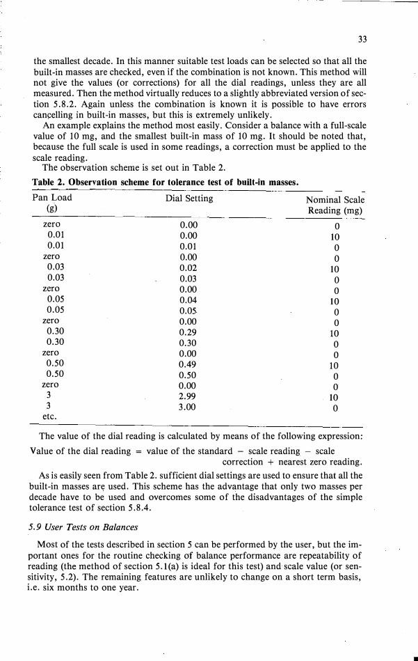
I J I ':.,!

32

This formula yields the amount that must be added to the balance reading to give

the correct value whenever this dial setting is used. The value of 'C' may be positive or negative. If m i, m2 are scale readings only and not dial readings plus scale readings, then the value of the dial setting must be subtracted from equation (12) to give the correction (see section 5.10. 7(a). Usually the value of the standard is closely similar to the value of the dial setting and it is not necessary to apply any corrections for the scale.

This method does not provide any safeguards against misreading the balance or arithmetical errors, but it has the advantage of being relatively easy and straightforward to use even though the results may not always be self consistent.

5.8.3 Least-squares calibration Each decade in the balance generally has four masses to make up the nine, or

more, combinations for the dial settings. To make use of this information in the least-squares analysis, the appropriate combination for the balance under test must be obtained either by observation or from the manufacturer. There are over 50 possible combinations used in different balances by different manufacturers. The least-squares method requires the observations obtained in section 5.8.2. However the calculations are fairly involved and for this reason chapter 9 is devoted to explaining them (see Humpries, 1960; Bell, 1955).

The least-squares method does have a number of advantages over all other methods: (i) it is the most accurate method;(ii) a self-consistent set of values is obtained;(iii) the standard deviation of the correction for each dial setting can be obtained if

desired;(iv) arithmetical errors and misreadings can be detected from an examination of the

residuals . .If the masses in the balance are required to be known to this accuracy then con­

sideration should be given to measuring by substitution with a calibrated set of masses. This should not involve any extra time, because to make use of the accuracy of the in-built masses a number of repeated readings must be made.

5. 8.4 Simple tolerance testIn general, there are very few balance users who actually apply corrections for the

dial readings. Most want to know whether the corrections to the dial readings con­form to the tolerances laid down by the manufacturer, or whether the balance is suf­ficiently accurate for their purpose.

The quickest way to do this is to set the dial reading so that all the built-in masses are lifted from the beam (e.g. position 9 or 99 etc.), place standards of equivalent value on the pan, and read the difference. It is possible (although unlikely) to have two large errors which cancel. In some combinations not all the masses are lifted off at position 9 and a second dial setting is required to ensure that this happens. These possibilities can be eliminated by taking more time and using the methods outlined in 5.8.2, 5.8.3 and 5.8.5. If the combination for a particular balance is known then all the masses can be lifted by using two dial settings. Unfortunately, the same two dial settings will not lift all masses for all balances.

5. 8. 5 Comprehensive tolerance testThis is basically the method proposed in ASTM E319. Two combinations of the

builtsin masses are compared with one calibrated mass. One dial setting has the same nominal value as the test mass; the other will be smaller by one step on the dial for

33

the smallest decade. In this manner suitable test loads can be selected so that all the

built-in masses are checked, even if the combination is not known. This method will not give the values (or corrections) for all the dial readings, unless they are all measured. Then the method virtually reduces to a slightly abbreviated version of sec­tion 5.8.2. Again unless the combination is known it is possible to have errors cancelling in built-in masses, but this is extremely unlikely.

An example explains the method most easily. Consider a balance with a full-scale value of 10 mg, and the smallest built-in mass of 10 mg. It should be noted that, because the full scale is used in some readings, a correction must be applied to the

scale reading. The observation scheme is set out in Table 2.

Table 2. Observation scheme for tolerance test of built-in masses.

Pan Load Dial Setting Nominal Scale (g) Reading (mg)

zero 0.00 0 0.01 0.00 10 0.01 0.01 0

zero 0.00 0 0.03 0.02 10 0.03 0.03 0

zero 0.00 0 0.05 0.04 10 0.05 0.05 0

zero 0.00 0 0.30 0.29 10 0.30 0.30 0

zero 0.00 0 0.50 0.49 10 0.50 0.50 0

zero 0.00 0 3 2.99 10 3 3.00 0

etc.

The value of the dial reading is calculated by means of the following expression:

Value of the dial reading = value of the standard - scale reading - scale correction + nearest zero reading.

As is easily seen from Table 2. sufficient dial settings are used to ensure that all the built-in masses are used. This scheme has the advantage that only two masses per decade have to be used and overcomes some of the disadvantages of the simple tolerance test of section 5.8.4.

5. 9 User Tests on Balances

Most of the tests described in section 5 can be performed by the user, but the im­

portant ones for the routine checking of balance performance are repeatability of reading (the method of section 5. l(a) is ideal for this test) and scale value (or sen­sitivity, 5.2). The remaining features are unlikely to change on a short term basis, i.e. six months to one year.

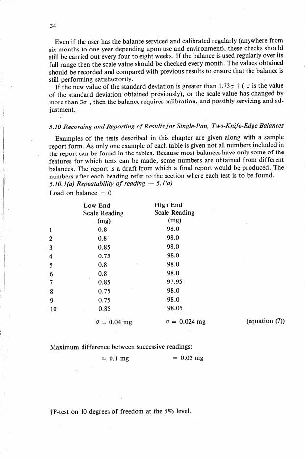
11 :11

,1· '''i

34

Even if the user has the balance serviced and calibrated regularly (anywhere from

six months to one year depending upon use and environment), these checks should

still be carried out every four to eight weeks. If the balance is used regularly over its

full range then the scale value should be checked every month. The values obtained

should be recorded and compared with previous results to ensure that the balance is

still performing satisfactorily. If the new value of the standard deviation is greater than 1.73a t ( a is the value

of the standard deviation obtained previously), or the scale value has changed by

more than 3 a , then the balance requires calibration, and possibly servicing and ad­

justment.

5. JO Recording and Reporting of Results for Single-Pan, Two-Knife-Edge Balances

Examples of the tests described in this chapter are given along with a sample

report form. As only one example of each table is given not all numbers included in

the report can be found in the tables. Because most balances have only some of the

features for which tests can be made, some numbers are obtained from different

balances. The report is a draft from which a final report would be produced. The

numbers after each heading refer to the section where each test is to be found.

5.10.l(a) Repeatability of reading - 5.l(a)

Load on balance = 0

Low End High End

Scale Reading Scale Reading (mg) (mg)

1 0.8 98.0

2 0.8 98.0

3 0.85 98.0

4 0.75 98.0

5 0.8 98.0

6 0.8 98.0

7 0.85 97.95

8 0.75 98.0

9 0.75 98.0

10 0.85 98.05

a= 0.04 mg a= 0.024 mg (equation (7))

Maximum difference between successive readings:

= O:l mg = 0.05 mg

tF-test on 10 degrees of freedom at the 5% level.

35

5.10.l(b) Repeatability of reading - 5.l(b)

M = 500 g

Number Pan Load Scale Difference Reading r = m-z

(mg) (mg)

1 0 Z1 1.0

M m1 1.3 r1 0.3

2 0 1.2

M 1.5 0.3

3 0 1.3

M 1.6 0.3

4 0 1.2

M 1.6 0.4

5 0 1.25

M 1.6 0.35

6 0 1.3

M 1.6 0.3

7 0 1.3

M 1.7 0.4

8 0 1.3

M 1.5 0.2

9 0 1.4

M 1.6 0.2

10 0 1.3

M 1.5 0.2

<J= 0.076mg (equation (8))

Maximum difference between successive readings = 0.2 mg

(iiliJJ

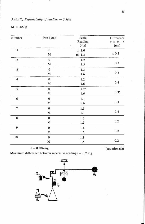
-1 I ,

'I

34

Even if the user has the balance serviced and calibrated regularly (anywhere from six months to one year depending upon use and environment), these checks should still be carried out every four to eight weeks. If the balance is used regularly over its full range then the scale value should be checked every month. The values obtained should be recorded and compared with previous results to ensure that the balance is still performing satisfactorily.

If the new value of the standard deviation is greater than 1.73a t ( er is the value of the standard deviation obtained previously), or the scale value has changed by more than 3 a , then the balance requires calibration, and possibly servicing and ad­justment.

5.10 Recording and Reporting of Results for Single-Pan, Two-Knife-Edge Balances

Examples of the tests described in this chapter are given along with a sample report form. As only one example of each table is given not all numbers included in the report can be found in the tables. Because most balances have only some of the features for which tests can be made, some numbers are obtained from different balances. The report is a draft from which a final report would be produced. The numbers after each heading refer to the section where each test is to be found. 5.10.l(a) Repeatability of reading - 5.l(a)

Load on balance = 0

Low End High End Scale Reading Scale Reading

(mg) (mg)

1 0.8 98.0

2 0.8 98.0

3 0.85 98.0

4 0.75 98.0

5 0.8 98.0

6 0.8 98.0

7 0.85 97.95

8 0.75 98.0

9 0.75 98.0

10 0.85 98.05

er= 0.04 mg a= 0.024 mg (equation (7))

Maximum difference between successive readings:

= 0.1 mg = 0.05 mg

tF-test on 10 degrees of freedom at the 5% level.

35

5.10.l(b) Repeatability of reading - 5.l(b)

M = 500 g

Number Pan Load Scale Difference Reading r = m-z

(mg) (mg)

1 0 Z1 1.0

M ml 1.3 r1 0.3

2 0 1.2

M 1.5 0.3

3 0 1.3

M 1.6 0.3

4 0 1.2

M 1.6 0.4

5 0 1.25

M 1.6 0.35

6 0 1.3

M 1.6 0.3

7 0 1.3

M 1.7 0.4

8 0 1.3

M 1.5 0.2

9 0 1.4

M 1.6 0.2

10 0 1.3

M 1.5 0.2

a= 0.076mg (equation (8))

Maximum difference between successive readings = 0.2 mg

[iIIID

I : ' '

36

5.10.2 Scale Value - 5.2

Calibrating Mass M = 0.100 017 g

Pan Load

Zero M

M

Zero

Scale Reading

z 0.0000 m 0.0996 m 0.0995 z 0.000 05

Correction = M - (m -z) = 0.000 49 g = 0.49 mg

Uncertainty= 3[(10-5/3)2 + (0.04 x 10-3)2/2F'

=8.6 xl0-5 g = 0.086 mg

5. J0.3(a) Uniformity of scale - 5.3.1

Pan Load Scale Reading Means

0 0.0000 M(0.020 05) 0.0199 0.0000 M 0.0199 0.0199 0 0.0000

2M(0.040 03) 0.0398 0.0000 2M 0.0398 0.0398 0 0.0000

3M(0.059 92) 0.0598 0.000 075 3M 0.0596 0.0597 0 0.000 15

4M(0.079 97) 0.0798 0.0002 4M 0.0798 0.0798 0 0.000 25

5M(0.100 02) 0.0998 0.000 225 5M 0.0997 0.099 75 0 0.0002

Maximum correction = 0.000 50 g

Difference

0.0199

0.0398

0.059 625

0.0796

0.099 525

Uncertainty = 3[(10-5/3)2 + (0.04 x 10-3)2f2] V2

= 8.6 X 10- 5 g = 0.086 mg

(equation (25))

Scale Correction = Mass - Difference

(g)

+ 0.000 15

+ 0.000 23

+ 0.000 30

+ 0.000 37

+ 0.000 50

(equation (25))

37

5.J0.3(b) Uniformity of scale - 5.3.2

Calibrating Mass M = 0.020 05 g Note: M' ""'M

Pan Scale Load Reading

0 0.0000 M 0.0200 M 0.0199 0 -0.0001

M' 0.0200M' + M 0.0401 M' + M 0.0399

M' 0.0200

2M' 0.0400 2M' + M 0.059 95 2M' + M 0.059 95

2M' 0.0401

3M' 0.0600 3M' + M 0.0798 3M' + M 0.0798

3M' 0.0598

4M' 0.0800 4M' + M 0.099 95 4M' + M 0.099 95

4M' 0.0799

Means Difference Scale Correction Cumulative M - difference Correction

-0.000 05

0.019 95

0.0200

0.0400

0.040 05

0.059 95

0.0599

0.0798

0.079 95

0.099 95

0.0199

0.0200

0.0199

0.0199

0.0200

+0.000 15

+0.000 05

+0.000 15

+0.000 15

+0.000 05

Maximum correction = 0.000 55 g

Uncertainty - see section 5 .10.3(a)

0.000 15

0.000 20

0.000 35

0.000 50

0.000 55

36

5.10.2 Scale Value - 5.2

Calibrating Mass M = 0.100 017 g

Pan Load

Zero M M

Zero

Scale Reading

z 0.0000 m 0.0996 m 0.0995 z 0.000 05

Correction = M - (m -z) = 0.000 49 g = 0.49 mg

Uncertainty= 3 [(10-5/3)2 + (0.04 x 10-3)2/2] Yi

= 8.6 x 10- 5 g = 0.086 mg

5. J0.3(a) Uniformity of scale - 5.3.1

Pan Load Scale Reading Means

0 0.0000 M(0.020 05) 0.0199 0.0000 M 0.0199 0.0199 0 0.0000

2M(0.040 03) 0.0398 0.0000 2M 0.0398 0.0398 0 0.0000

3M(0.059 92) 0.0598 0.000 075

3M 0.0596 0.0597

0 0.000 15 4M(0.079 97) 0.0798 0.0002 4M 0.0798 0.0798 0 0.000 25

5M(0.100 02) 0.0998 0.000 225

5M 0.0997 0.099 75

0 0.0002

Maximum correction = 0.000 50 g

Difference

0.0199

0.0398

0.059 625

0.0796

0.099 525

Uncertainty = 3[(10- 5/3)2 + (0.04 x 10-3)2f2] Y' = 8.6 X 10- 5 g = 0.086 mg

(equation (25))

Scale Correction = Mass - Difference

(g)

+ 0.000 15

+ 0.000 23

+ 0.000 30

+ 0.000 37

+ 0.000 50

(equation (25))

37

5.10.3(b) Uniformity of scale - 5.3.2

Calibrating Mass M = 0.020 05 g Note: M' ""M

Pan Scale Means Difference Scale Correction Cumulative Load Reading M - difference Correction

0 0.0000 M 0.0200 -0.000 05

M 0.0199 0.0199 +0.000 15 0.000 15

0 -0.0001 0.019 95

M' 0.0200M' + M 0.0401 0.0200

M' + M 0.0399 0.0200 +0.000 05 0.000 20

M' 0.0200 0.0400

2M' 0.0400 2M' + M 0.059 95 0.040 05

2M' + M 0.059 95 0.0199 +0.000 15 0.000 35

2M' 0.0401 0.059 95

3M' 0.0600 3M' + M 0.0798 0.0599

3M' + M 0.0798 0.0199 +0.000 15 0.000 50

3M' 0.0598 0.0798

4M' 0.0800 4M' + M 0.099 95 0.079 95

4M' + M 0.099 95 0.0200 +0.000 05 0.000 55

4M' 0.0799 0.099 95

Maximum correction = 0.000 55 g

Uncertainty - see section 5.10.3(a)

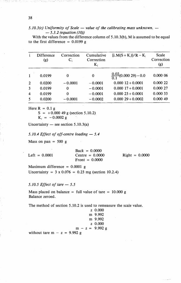
38

5.10.3(c) Uniformity of Scale - value of the calibrating mass unknown. -- 5.3.2 (equation (10))

With the values from the difference column of 5 .10. 3 (b ), M is assumed to be equal to the first difference = 0.0199 g

Difference Correction Cumulative (g) ci Correction

Ki

1 0.0199 0 0

2 0.0200 -0.0001 -0.0001

3 0.0199 0 -0.0001

4 0.0199 0 -0.0001

5 0.0200 -0.0001 -0.0002

Here R = 0.1 g S = +0.000 49 g (section 5.10.2)K, = -0.0002 g

Uncertainty - see section 5.10.3(a)

5.10.4 Effect of off�centre loading - 5.4

Mass on pan = 500 g

Left = 0.0001 Back = 0.0000 Centre = 0.0000 Front = 0.0000

Maximum difference = 0.0001 g

[i.M(S + K,)]/R -Ki

g:?2(0.000 29)-0.0

0.000 12 + 0.0001

0.000 17 + 0.0001

0.000 23 + 0.0001

0.000 29+0.0002

Right = 0.0000

Uncertainty = 3 x 0.076 = 0.23 mg (section 10.2.4)

5.10.5 Effect of tare - 5.5

Mass placed on balance = full value of tare = 10.000 g Balance zeroed.

The method of section 5.10.2 is used to remeasure the scale value. z 0.000

m 9.992 m 9.992 z 0.000

m - z = 9.992 g without tare m - z = 9.992 g

Scale Correction

(g)

0.000 06

0.000 22

0.000 27

0.000 33

0.000 49

r--

5.10.6 Hysteresis - 5.6

M (half capacity of balance) = 500 g

Pan Load

Zero Z1

M m1 M + M' M m2

Zero Zz

1

0.0000 500.000 25 700.000 25 500.0002 -0.0002

2

0.0000 500.000 35 700.0004 500.0004

0.000 05

Hysteresis = m1 - m2 = 0.0000 and z1 - z2 = 0.0000

Uncertainty = 3 x 0.076/6Y, = 0.10 mg

39

3

0.0000 500.0002 700.0003 500.000 25

0.0000

Note: The factor 1/6Yi occurs because the measurement is effectively double weighing repeated 3 times - see equation (25).

, I

38

5.10.3(c) Uniformity of Scale - value of the calibrating mass unknown. -- 5.3.2 (equation (JO))

With the values from the difference column of 5 .10.3 (b ), M is assumed to be equal to the first difference = 0.0199 g

Difference Correction Cumulative (g) ci Correction

Ki

1 0.0199 0 0

2 0.0200 -0.0001 -0.0001

3 0.0199 0 -0.0001

4 0.0199 0 -0.0001

5 0.0200 -0.0001 -0.0002

Here R = 0.1 g S = +0.000 49 g (section 5.10.2)Kr = -0.0002 g

Uncertainty - see section 5.10.3(a)

5.10.4 Effect of off�centre loading - 5.4

Mass on pan = 500 g

Left = 0.0001 Back = 0.0000 Centre = 0.0000 Front = 0.0000

Maximum difference = 0.0001 g

[i.M(S + Kr)]/R - Ki

g:�2(0.000 29) -0.0

0.000 12 + 0.0001

0.000 17 + 0.0001

0.000 23 + 0.0001

0.000 29 + 0.0002

Right = 0.0000

Uncertainty = 3 x 0.076 = 0.23 mg (section 10.2.4)

5.10.5 Effect of tare - 5.5

Mass placed on balance = full value of tare = 10.000 g Balance zeroed.

The method of section 5.10.2 is used to remeasure the scale value. z 0.000

m 9.992 m 9.992 z 0.000

m - z = 9.992 g without tare m - z = 9.992 g

Scale Correction

(g)

0.000 06

0.000 22

0.000 27

0.000 33

0.000 49

5.10.6 Hysteresis - 5.6

M (half capacity of balance) = 500 g

Pan Load

Zero Z1 M m1 M + M' M m2

Zero Zz

1

0.0000 500.000 25 700.000 25 500.0002 -0.0002

2

0.0000 500.000 35 700.0004 500.0004

0.000 05

Hysteresis = m1 - m2 = 0.0000 and z 1 - z2 = 0.0000

Uncertainty = 3 x 0.076/6Y> = 0.10 mg

39

3

0.0000 500.0002 700.0003 500.000 25

0.0000

Note: The factor 1/6Y> occurs because the measurement is effectively double weighing repeated 3 times - see equation (25).

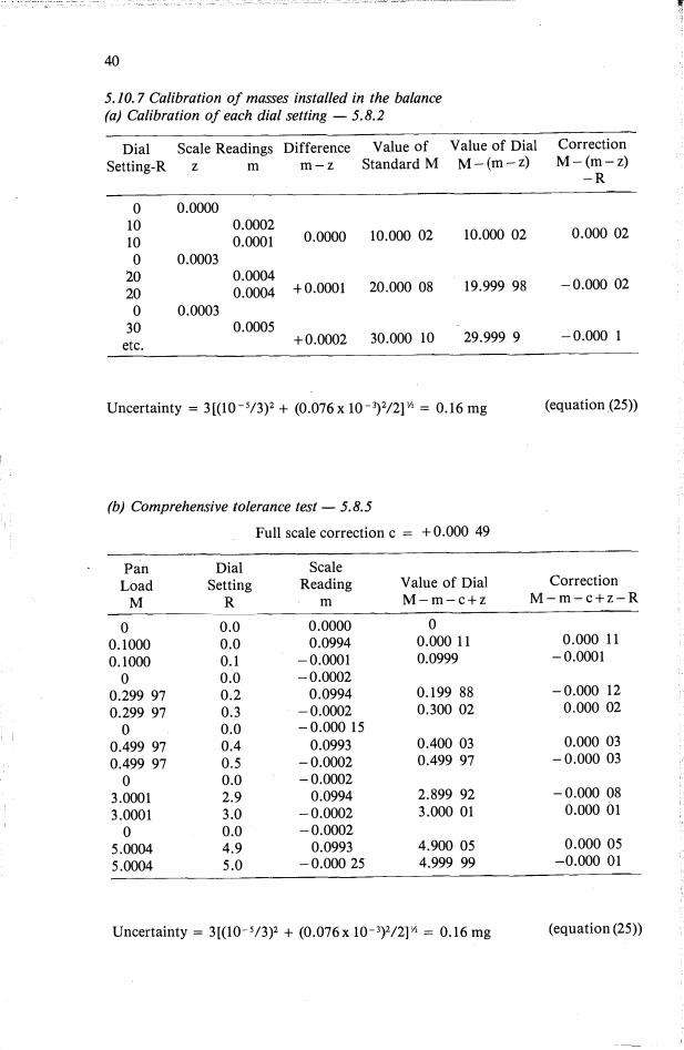
r-·,

40

5.10. 7 Calibration of masses installed in the balance

(a) Calibration of each dial setting - 5.8.2

Dial Scale Readings Difference Value of Value of Dial Correction

Setting-R z m m-z Standard M M-(m-z) M-(m-z) -R

0 0.0000 10 0.0002 10 0.0001 0.0000 10.000 02 10.000 02 0.000 02

0 0.0003 20 0.0004

20 0.0004 +0.0001 20.000 08 19.999 98 -0.000 02

0 0.0003 30 0.0005

etc. +0.0002 30.000 10 29.999 9 -0.000 1

Uncertainty= 3[(10- 5/3)2 + (0.076x 10- 3)2/2] v, = 0.16 mg (equation (25))

(b) Comprehensive tolerance test - 5.8.5

Full scale correction c = +0.000 49

Pan Dial Scale

/i

Load Setting Reading Value of Dial Correction

M R m M-m-c+z M-m-c+z-R

0 0.0 0.0000 0

0.1000 0.0 0.0994 0.000 11 0.000 11

0.1000 0.1 -0.0001 0.0999 -0.0001

0 0.0 -0.0002

0.299 97 0.2 0.0994 0.199 88 -0.000 12

0.299 97 0.3 -0.0002 0.300 02 0.000 02

0 0.0 -0.000 15

0.499 97 0.4 0.0993 0.400 03 0.000 03

0.499 97 0.5 -0.0002 0.499 97 -0.000 03

0 0.0 -0.0002

3.0001 2.9 0.0994 2.899 92 -0.000 08

3.0001 3.0 -0.0002 3.000 01 0.000 01

0 0.0 -0.0002

5.0004 4.9 0.0993 4.900 05 0.000 05

5.0004 5.0 -0.000 25 4.999 99 -0.000 01

Uncertainty= 3[(10- 5/3)2 + (0.076 x 10- 3)2/2] Y2 = 0.16 mg (equation (25))

:1

,--

5.10.8 Sample Report on a two-knife-edge balance

REPORT ON

41

SINGLE-PAN TWO-KNIFE-EDGE BALANCE

Maker Mettler Model B5 CJOOO Serial No. 654321

Scale Division J mg Capacity 1000 g Scale Range J 00 mg Reading to 0.1 mg by means of optical readout Type (top-loading or analytical) analytical

Client CSIRO Examined at (precise location) Room C261, National Measurement Laboratory Temperature of test 20. 5 °C

Repeatability of Reading

Load

zero

half maximum 500 g

maximum 1000 g

Scale Reading

0

100

0

100

100

Uniformity of Scale

Scale Reading (mg)

Correction (mg)

Uncertainty ( ±) (mg)

Off-Centre Loading

Standard Deviation of reading (mg)

0.04 0.03

0.08

0.09

0.10

Maximum difference between successive readings (mg)

0.10

0.05

0.20

0.25

0.30

20 40 60 80 JOO

+ 0.15 + 0.25 + 0.30 + 0.35 + 0.50

A mass of approximately 500 g was placed on a disk of 50 mm diameter and mov­ed to the positions on the pan as specified. The balance readings obtained are given in the table.

Beginning of scale

End of scale

Centre

0.0

0.0

Front Back

0.0 0.0

0.0 0.1

Left Right Maximum difference

0.1 0.0 0.1 mg

0.1 0.0 0.1 mg

ii

40

5.10. 7 Calibration of masses installed in the balance

(a) Calibration of each dial setting - 5.8.2

Dial Scale Readings Difference Value of Value of Dial Correction

Setting-R z m m-z Standard M M-(m-z) M-(m-z) -R

0 0.0000 10 0.0002 10 0.0001 0.0000 10.000 02 10.000 02 0.000 02

0 0.0003 20 0.0004

20 0.0004 +0.0001 20.000 08 19.999 98 -0.000 02

0 0.0003 30 0.0005

etc. +0.0002 30.000 10 29.999 9 -0.000 1

Uncertainty= 3[(10- 5/3)2 + (0.076x 10- 3)2/2] v, = 0.16 mg (equation (25))

(b) Comprehensive tolerance test - 5.8.5

Full scale correction c = +0.000 49

Pan Dial Scale

Load Setting Reading Value of Dial Correction

M R m M-m-c+z M-m-c+z-R

0 0.0 0.0000 0

0.1000 0.0 0.0994 0.000 11 0.000 11

0.1000 0.1 -0.0001 0.0999 -0.0001

0 0.0 -0.0002

0.299 97 0.2 0.0994 0.199 88 -0.000 12

0.299 97 0.3 -0.0002 0.300 02 0.000 02

0 0.0 -0.000 15

0.499 97 0.4 0.0993 0.400 03 0.000 03

0.499 97 0.5 -0.0002 0.499 97 -0.000 03

0 0.0 -0.0002

3.0001 2.9 0.0994 2.899 92 -0.000 08

3.0001 3.0 -0.0002 3.000 01 0.000 01

0 0.0 -0.0002

5.0004 4.9 0.0993 4.900 05 0.000 05

5.0004 5.0 -0.000 25 4.999 99 -0.000 01

Uncertainty= 3[(10- 5/3)2 + (0.076 x 10- 3)2/2] v, = 0.16 mg (equation (25))

i.----

5.10.8 Sample Report on a two-knife-edge balance

REPORT ON

41

SINGLE-PAN TWO-KNIFE-EDGE BALANCE

Maker Mettler Model B5 ClOOO Capacity J OOO g Scale Range 100 mg Reading to 0.1 mg by means of optical readout Type (top-loading or analytical) analytical Client CSIRO

Serial No. 654321 Scale Division 1 mg

Examined at (precise location) Room C261, National Measurement Laboratory Temperature of test 20.5 °C

Repeatability of Reading

Load

zero

half maximum

500 g

maximum 1000 g

Scale Reading

0 100

0

100

100

Uniformity of Scale

Scale Reading (mg)

Correction (mg)

Uncertainty ( ±) (mg)

Off-Centre Loading

Standard Deviation of reading (mg)

0.04 0.03

0.08

0.09

0.10

Maximum difference between successive readings (mg)

0.10

0.05

0.20

0.25

0.30

20 40 60 80 JOO

+0.15 +0.25 +0.30 +0.35 +0.50

A mass of approximately 500 g was placed on a disk of 50 mm diameter and mov­ed to the positions on the pan as specified. The balance readings obtained are given in the table.

Beginning of scale

End of scale

Centre

0.0

0.0

Front Back

0.0 0.0

0.0 0.1

Left Right Maximum difference

0.1 0.0 0.1 mg

0.1 0.0 0.1 mg

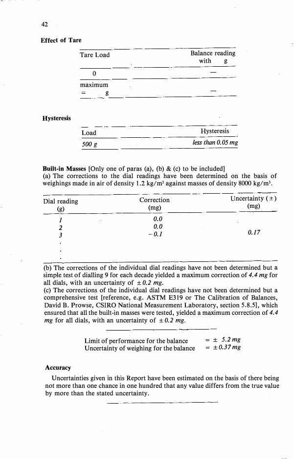
1,

' I

! !

42

Effect of Tare

Hysteresis

Tare Load

0

maximum g

Load

500 g

Balance reading with g

Hysteresis

less than 0. 05 mg

Built-in Masses [Only one of paras (a), (b) & (c) to be included] (a) The corrections to the dial readings have been determined on the basis ofweighings made in air of density 1.2 kg/m3 against masses of density 8000 kg/m3

•

Dial reading (g)

1

2

3

Correction (mg)

0.0

0.0

-0.1

Uncertainty ( ±) (mg)

0.17

(b) The corrections of the individual dial readings have not been determined but asimple test of dialling 9 for each decade yielded a maximum correction of 4.4 mg forall dials, with an uncertainty of ± 0.2 mg.(c) The corrections of the individual dial readings have not been determined but acomprehensive test [reference, e.g. ASTM E319 or The Calibration of Balances,David B. Prowse, CSIRO National Measurement Laboratory, section 5.8.51, whichensured that all the built-in masses were tested, yielded a maximum correction of 4.4

mg for all dials, with an uncertainty of ± 0.2 mg.

Accuracy

Limit of performance for the balance Uncertainty of weighing for the balance

= ± 5.2 mg == ±0.37mg

Uncertainties given in this Report have been estimated on the basis of there being not more than one chance in one hundred that any value differs from the true value by more than the stated uncertainty.

Notes 1. The balance has been tested according to the specifications laid down in

The Calibration of Balances David B. Prowse

CSIRO National Measurement Laboratory Chapter 5.

2. A reading consists of [delete (a) or (b) as appropriate](a) releasing the balance without disturbing· th0 load.

43

(b) removing the load between each reading and using the difference between thereading and zero in the calculations.3. When the sign of the correction is positive (+) the amount should be added to thescale reading to give the correct value and when negative ( - ) subtracted from it.4. Air buoyancy corrections should be calculated on the basis that the object beingweighed is balanced against a hypothetical mass of density 8000 kg/m3 in air ofmeasured density.5. The Limit of Performance is the tolerance band within which all readings of thebalance will fall.

6. Calibration of Electromagnetic-Force-Compensation Balances

These balances have an electronic display and sometimes the reading is such thatthe last digit will flick continually between two successive numbers. When this hap­pens the reading used should be the mean of the two digits.

6. 1 Scale Value

For balances operating on the principle of electromagnetic force compensationthe idea of sensitivity needs to be modified slightly. The electronic display covers the whole weighing range of the balance and by adjustment, and the use of a standard mass, this display can be made equal to its nominal value at any one point. At other points linearity and other errors may cause the output to depart from its nominal value. So rather than refer to sensitivity it is preferable to talk of departures from nominal reading or linearity. Rather than measure the sensitivity, the scale value is set using a standard mass, either exterior or interior to the balance, so that at this load each digit represents an exact fraction of a gram. Then the departures from nominal value at other. loads are measured (section 6.2).

6.1.1 Calibration The balance is calibrated by placing a known mass (usually maximum capacity) on

the pan and adjusting the balance until it displays the value of the mass. Some balances have a built-in calibrating mass or an automatic calibrating cycle. Whatever the system all balances should be checked to ensure that the calibration is correct and that the calibration mass is unchanged (section 6.8). 6.1.2 Effect of gravity

Because these balances measure force, the calibration will vary with gravity and the scale value must be adjusted when the balance is moved from one place to another. A standard mass must be used to adjust the scale value as it is not con­sidered adequate to apply corrections for change in the gravitational field. The value of g, local gravity, varies with both latitude and local anomalies. If the balance has been transported sufficiently far for the value of g to be different, then there is a real possibility that the calibration has changed due to vibration, levelling, etc., and it should be recalibrated as a matter of course (see also section 6. 7 .6).

42

Effect of Tare

Hysteresis

Tare Load

0

maximum g

Load

500 g

Balance reading with g

Hysteresis

less than 0. 05 mg

Built-in Masses [Only one of paras (a), (b) & (c) to be included] (a) The corrections to the dial readings have been determined on the basis ofweighings made in air of density 1.2 kg/m3 against masses of density 8000 kg/m3

•

Dial reading (g)

1

2

3

Correction (mg)

0.0 0.0

-0.1

Uncertainty ( ±) (mg)

0.17

(b) The corrections of the individual dial readings have not been determined but asimple test of dialling 9 for each decade yielded a maximum correction of 4.4 mg forall dials, with an uncertainty of ± 0.2 mg.(c) The corrections of the individual dial readings have not been determined but acomprehensive test [reference, e.g. ASTM E319 or The Calibration of Balances,David B. Prowse, CSIRO National Measurement Laboratory, section 5.8.5], whichensured that all the built-in masses were tested, yielded a maximum correction of 4.4

mg for all dials, with an uncertainty of ± 0.2 mg.

Accuracy

Limit of performance for the balance Uncertainty of weighing for the balance

= ± 5.2mg == ±0.37mg

Uncertainties given in this Report have been estimated on the basis of there being not more than one chance in one hundred that any value differs from the true value by more than the stated uncertainty.

Notes 1. The balance has been tested according to the specifications laid down in

The Calibration of Balances David B. Prowse

CSIRO National Measurement Laboratory Chapter 5.

2. A reading consists of [delete (a) or (b) as appropriate](a) releasing the balance without disturbing· th@ load.

43

(b) removing the load between each reading and using the difference between thereading and zero in the calculations.3. When the sign of the correction is positive (+) the amount should be added to thescale reading to give the correct value and when negative ( - ) subtracted from it.4. Air buoyancy corrections should be calculated on the basis that the object beingweighed is balanced against a hypothetical mass of density 8000 kg/m3 in air ofmeasured density.5. The Limit of Performance is the tolerance band within which all readings of thebalance will fall.

6. Calibration of Electromagnetic-Force-Compensation Balances

These balances have an electronic display and sometimes the reading is such thatthe last digit will flick continually between two successive numbers. When this hap­pens the reading used should be the mean of the two digits.

6.1 Scale Value

For balances operating on the principle of electromagnetic force compensation the idea of sensitivity needs to be modified slightly. The electronic display covers the whole weighing range of the balance and by adjustment, and the use of a standard mass, this display can be made equal to its nominal value at any one point. At other points linearity and other errors may cause the output to depart from its nominal value. So rather than refer to sensitivity it is preferable to talk of departures from nominal reading or linearity. Rather than measure the sensitivity, the scale value is set using a standard mass, either exterior or interior to the balance, so that at this load each digit represents an exact fraction of a gram. Then the departures from nominal value at other. loads are measured (section 6.2).

6.1.1 Calibration The balance is calibrated by placing a known mass (usually maxirnum capacity) on

the pan and adjusting the balance until it displays the value of the mass. Some balances have a built-in calibrating mass or an automatic calibrating cycle. Whatever the system all balances should be checked to ensure that the calibration is correct and that the calibration mass is unchanged (section 6.8). 6.1.2 Effect of gravity

Because these balances measure force, the calibration will vary with gravity and the scale value must be adjusted when the balance is moved from one place to another. A standard mass must be used to adjust the scale value as it is not con­sidered adequate to apply corrections for change in the gravitational field. The value of g, local gravity, varies with both latitude and local anomalies. If the balance has been transported sufficiently far for the value of g to be different, then there is a real possibility that the calibration has changed due to vibration, levelling, etc., and it should be recalibrated as a matter of course (see also section 6.7.6).

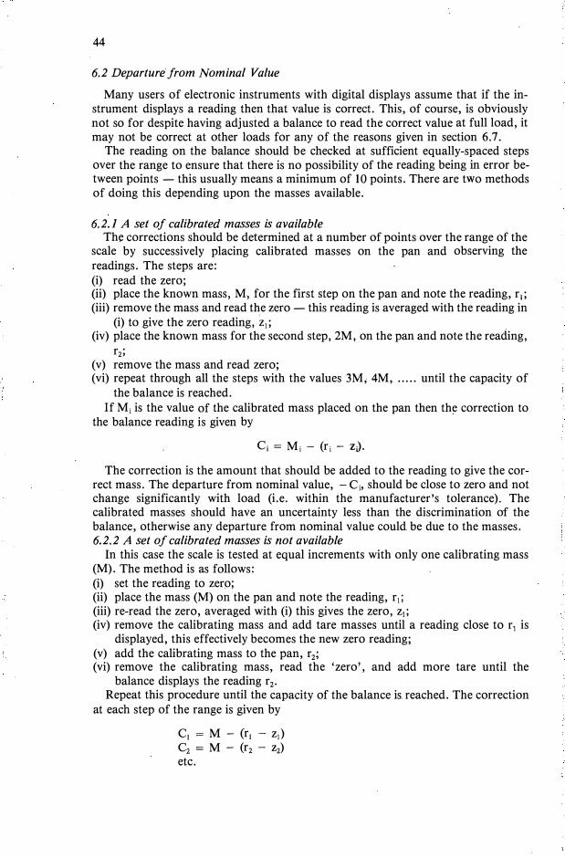
r

44

6.2 Departure from Nominal Value

Many users of electronic instruments with digital displays assume that if the in­strument displays a reading then that value is correct. This, of course, is obviously not so for despite having adjusted a balance to read the correct value at full load, it may not be correct at other loads for any of the reasons given in section 6.7.

The reading on the balance should be checked at sufficient equally-spaced steps over the range to ensure that there is no possibility of the reading being in error be­tween points - this usually means a minimum of 10 points. There are two methods of doing this depending upon the masses available.

6.2.1 A set of calibrated masses is available The corrections should be determined at a number of points over the range of the

scale by successively placing calibrated masses on the pan and observing the readings. The steps are: (i) read the zero;(ii) place the known mass, M, for the first step on the pan and note the reading, r1;

(iii) remove the mass and read the zero - this reading is averaged with the reading in(i) to give the zero reading, z1;

(iv) place the known mass for the second step, 2M, on the pan and note the reading,r2;

(v) remove the mass and read zero;(vi) repeat through all the steps with the values 3M; 4M, ..... until the capacity of

the balance is reached. If Mi is the value of the calibrated mass placed on the pan then the correction to

the balance reading is given by

Ci = M i - (r i - zJ.

The correction is the amount that should be added to the reading to give the cor­rect mass. The departure from nominal value, - Ci, should be close to zero and not change significantly with load (i.e. within the manufacturer's tolerance). The calibrated masses should have an uncertainty less than the discrimination of the balance, otherwise any departure from nominal value could be due to the masses. 6.2.2 A set of calibrated masses is not available

In this case the scale is tested at equal increments with only one calibrating mass (M). The method is as follows: (i) set the reading to zero;(ii) place the mass (M) on the pan and note the reading, r1 ;

(iii) re-read the zero, averaged with (i) this gives the zero, z1;

(iv) remove the calibrating mass and add tare masses until a reading close to r1 isdisplayed, this effectively becomes the new zero reading;

(v) add the calibrating mass to the pan, r2;

(vi) remove the calibrating mass, read the 'zero', and add more tare until thebalance displays the reading r2•

Repeat this procedure until the capacity of the balance is reached. The correction at each step of the range is given by

C1 = M - (r1 - z1) C2 = M - (r2 - z2) etc.

45

For these corrections to be equivalent to the values obtained in 6.2.1 the cumulative corrections must be calculated, i.e. C1 , C1 + C2 , C1 + C2 + C3 , etc. This method does not require any calibrated masses other than M, and although by its nature is more time consuming than the method of 6.2.1 it often provides more con­sistent values.

If the value of M is not known accurately then this method gives the non-linearity of the scale but the corrections will depart from their true value by a fixed but unknown amount, and so cannot be used to correct the reading on the balance. If M is an integer fraction of the range (i.e. M = r1 -z1 , giving C1 = 0), then the total cumulative correction can be equated to the scale value at full scale (section 6.1), and numerically accurate corrections obtained over the full range from equation (13).

The correction to the scale value has been set to zero (section 6.1), and so does not appear in the following equation (cf. equation (10)):

correction (i) = iMK/R - Ki

where R is the weighing range of the balance (i.e. full scale), K, is the calculated cumulative correction at full scale, Ki = C1 + C2 + .. . + Ci, i = 1, 2, ... numerical order of reading the balance.

6.2.3 Balances with built-in masses

(13)

Some electromagnetic-force-compensation balances have built-in masses which are applied automatically when the load exceeds a certain value. This value is dif­ferent, usually by some grams, for increasing and decreasing loads. It is therefore not really appropriate to consider the masses separately from the electronic range, but the departure from nominal value should be measured over the whole range. For these balances this should be done with the load both increasing and decreasing, so that any effect due to the hysteresis in the removal and replacement of the masses is measured. This is more difficult for decreasing load but can be done for both direc-tions by the following method: (i) read the zero;(ii) place the calibrating mass on the pan and note the reading;(iii) add a load sufficient to trigger the mechanism so that the next mass is removed

from the pan;(iv) remove the additional mass and note the reading;(v) remove the calibrating mass and read the zero;(vi) repeat steps (i) to (v) until the capacity of the balance is reached.

The corrections for increasing load and decreasing load are then calculated asdescribed in section 6.2.1. If the readings do not differ by more than twice the stan­dard deviation then they are not significantly different and the mean value can be reported.

The hysteresis test (section 6.5) is superfluous when this calibration is done.

6.3 Repeatability of Reading

This is a measure of how consistently a reading is displayed by the balance, and is usually expressed as a standard deviation, obtained from a series of repeated readings together with the relative size of the maximum difference between two suc­c_essive readings. There are a number of methods of measuring the standard devia­tion, but the method adopted should be realistic. Because these balances do not weigh at constant load the effect of different loads on the repeatability is likely to be

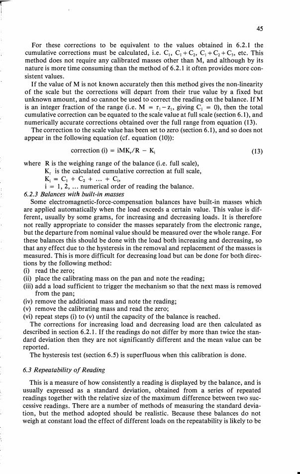
r

! i

44

6.2 Departure from Nominal Value

Many users of electronic instruments with digital displays assume that if the in­strument displays a reading then that value is correct. This, of course, is obviously not so for despite having adjusted a balance to read the correct value at full load, it may not be correct at other loads for any of the reasons given in section 6.7.

The reading on the balance should be checked at sufficient equally-spaced steps over the range to ensure that there is no possibility of the reading being in error be­tween points - this usually means a minimum of 10 points. There are two methods of doing this depending upon the masses available.

6.2.I A set of calibrated masses is available The corrections should be determined at a number of points over the range of the

scale by successively placing calibrated masses on the pan and observing the readings. The steps are: (i) read the zero;(ii) place the known mass, M, for the first step on the pan and note the reading, r1;(iii) remove the mass and read the zero - this reading is averaged with the reading in

(i) to give the zero reading, z1;(iv) place the known mass for the second step, 2M, on the pan and note the reading,

r2;(v) remove the mass and read zero;(vi) repeat through all the steps with the values 3M; 4M, ..... until the capacity of

the balance is reached. If Mi is the value of the calibrated mass placed on the pan then the correction to

the balance reading is given by

C i = Mi - (r i - zJ.

The correction is the amount that should be added to the reading to give the cor­rect mass. The departure from nominal value, -C i, should be close to zero and not change significantly with load (i.e. within the manufacturer's tolerance). The calibrated masses should have an uncertainty less than the discrimination of the balance, otherwise any departure from nominal value could be due to the masses. 6.2.2 A set of calibrated masses is not available

In this case the scale is tested at equal increments with only one calibrating mass (M). The method is as follows: (i) set the reading to zero;(ii) place the mass (M) on the pan and note the reading, r1 ;(iii) re-read the zero, averaged with (i) this gives the zero, z1;

(iv) remove the calibrating mass and add tare masses until a reading close to r1 isdisplayed, this effectively becomes the new zero reading;

(v) add the calibrating mass to the pan, r2;

(vi) remove the calibrating mass, read the 'zero', and add more tare until thebalance displays the reading r2•

Repeat this procedure until the capacity of the balance is reached. The correction at each step of the range is given by

C 1 = M - (r1 - z1) C2 = M - (r2 - z)etc.

·�·

45

For these corrections to be equivalent to the values obtained in 6.2.1 the cumulative corrections must be calculated, i.e. C 1, C 1 + C2, C 1 + C2 + C3, etc. This method does not require any calibrated masses other than M, and although by its nature is more time consuming than the method of 6.2.1 it often provides more con­sistent values.

If the value of M is not known accurately then this method gives the non-linearity of the scale but the corrections will depart from their true value by a fixed but unknown amount, and so cannot be used to correct the reading on the balance. If M is an integer fraction of the range (i.e. M = r1 -z1, giving C 1 = O), then the total cumulative correction can be equated to the scale value at full scale (section 6.1), and numerically accurate corrections obtained over the full range from equation (13).

The correction to the scale value has been set to zero (section 6.1), and so does not appear in the following equation (cf. equation (10)):

correction (i) = iMK/R - Ki

where R is the weighing range of the balance (i.e. full scale), Kr is the calculated cumulative correction at full scale, Ki = C 1 + C2 + ... + Ci, i = 1, 2, ... numerical order of reading the balance.

6.2.3 Balances with built-in masses

(13)

Some electromagnetic-force-compensation balances have built-in masses which are applied automatically when the load exceeds a certain value. This value is dif­ferent, usually by some grams, for increasing and decreasing loads. It is therefore not really appropriate to consider the masses separately from the electronic range, but the departure from nominal value should be measured over the whole range. For these balances this should be done with the load both increasing and decreasing, so that any effect due to the hysteresis in the removal and replacement of the masses is measured. This is more difficult for decreasing load but can be done for both direc-tions by the following method: (i) read the zero;(ii) place the calibrating mass on the pan and note the reading;(iii) add a load sufficient to trigger the mechanism so that the next mass is removed

from the pan;(iv) remove the additional mass and note the reading;(v) remove the calibrating mass and read the zero;(vi) repeat steps (i) to (v) until the capacity of the balance is reached.

The corrections for increasing load and decreasing load are then calculated asdescribed in section 6.2.1. If the readings do not differ by more than twice the stan­dard deviation then they are not significantly different and the mean value can be reported.

The hysteresis test (section 6.5) is superfluous when this calibration is done.

6.3 Repeatability of Reading

This is a measure of how consistently a reading is displayed by the balance, and is usually expressed as a standard deviation, obtained from a series of repeated readings together with the relative size of the maximum difference between two suc­c_essive readings. There are a number of methods of measuring the standard devia­

t10n, but the method adopted should be realistic. Because these balances do not weigh at constant load the effect of different loads on the repeatability is likely to be

I' I

46

more significant than for substitution balances, and so the repeatability of reading should be measured at more than one load.

All weighings involve a minimum of two readings - a zero reading and a reading with the mass to be measured. If this difference is measured a number of times it is a good measure of the repeatability of reading.

Thus the standard deviation is calculated from the difference between the zero reading (z;) and the reading with a mass M on the pan (m;), i.e. r; = m; - Z;. Therefore

a = [ 2 (r; - f)2/(n -1)) v, i

i = l, ... ,n (14)

The minimum number of readings for estimating the repeatability of reading is 10. The balance should not be zeroed during this series of readings. This procedureis then repeated for a number of different values of M, preferably near zero, halfmaximum and maximum load. For these cases the standard deviation is calculatedindividually rather than as a combined standard deviation by means of equation (3).It is possible to apply statistical tests to decide whether they should be combined but,because of the accuracy involved, this is not considered necessary. The largest valueshould be selected as the standard deviation of the balance.

Most electromagnetic-force-compensation balances, as distinct from knife-edge balances, are arranged so that the accuracy of the balance is equal to, or greater than, the discrimination. This means that when the balance is tested the same value may be obtained for all the readings. In this case the standard deviation as calculated by equation (14) is zero.

It can be shown that if one of the n readings departs from zero by dx then the stan­dard deviation is given by:

If dx = 1 digit, as is the usual case, then for n = 10 the standard deviation is approximately one-third of the discrimination of the balance. Hence to be realistic, this should be the minimum standard deviation quoted for the balance.

6.4 Effect of Off-Centre Loading

When the centre of mass of the object being weighed is off-centre on the pan, shift or corner-load error may occur. It is difficult to produce figures that can be used to correct the balance readings because the effect is not always linear with respect to either load or position. This test is designed to enable the user to decide how ac­curately objects must be positioned on the pan for this effect to be negligible. As these balances require some form of mechanical parallel linkage to transfer the load on the pan to the transducer, the effect of off-centre or corner loading may be quite significant.

This effect is most easily measured by placing a mass on the centre of the pan and then moving it successively to the front, rear, left and right positions on the pan, noting the reading each time. Accurate masses are not required; any suitable piece of turned brass or stainless steel is adequate.

Problems arise as to the magnitude of the mass placed on the pan, its shape and how far it should be moved. (i) Most balance manufacturers recommend that the effect be measured at approxi-

47

mately one-third or one-half the maximum load of the balance, or they quote per­formance figures at this load. Because this effect is often non-linear, measurement at a larger load will not necessarily give a larger reading. Also placing a large mass near the edge of the pan could possibly do some damage to the mechanism. Hence it is recommended that the test be carried out at the load recommended by the manufacturer, or if this is not known, then it should be at approximately one-third the maximum capacity of the balance. It is stressed that a single mass should be used for this test, and this restricts the choice to. values of 1, 2, 5 and perhaps 3 (unless special masses are available). For example, a balance of 1200 g capacity should be tested with a 500 g mass, because 200 g is too small. (ii) Masses from different manufacturers differ in shape so that when their edges arealigned with the edge of the pan the centres of mass will be different distances fromthe pan centre. For balances up to 10 kg capacity this problem can be overcome if adisc of light material (aluminium, perspex, etc.) of dimensions 10 mm by 50 mmdiameter is placed on the pan and the mass placed on top. The disc can always bemoved the same distance regardless of the shape of the mass. For analytical typebalances and those with a pan diameter less than 100 mm, a 20 mm disc of conduct­ing material (to eliminate effects of static electricity) should be used. A disc need notbe used for balances of capacity greater than 10 kg.(iii) The observed error depends crucially upon how far the mass is moved. Balancemanufacturers move the mass to the lip of the pan, defined as that area where theflat surface of the pan starts to curve up. This is considered the best position. Insome cases it is possible for the mass on the disc to overhang the edge of the pan dur­ing the test. This is unlikely to be serious provided the test mass is no more than one­third of the capacity, and should not affect the values obtained.

Some users change or modify their pans. In these cases an attempt should be made to carry out and report the test in a logical way.

6.5 li)'steresis

A properly adjusted balance in good condition should show no more hysteresis than 1 count. If the balance shows more hysteresis than this then it needs either ad­justing or cleaning. It is only necessary to test for hysteresis a few times during the life of the balance.

Testing at one point, about mid-range, is adequate. Proceed as follows: (i) zero the balance, z 1 ;

(ii) place a mass M, equal to half the range, on the pan, m1

;

(iii) add extra mass to bring the balance reading close to full range;(iv) remove the extra mass and read the balance with M still on the pan, m2;

(v) remove M and read the zero, z2 •

Repeat the above procedure three times and average the differences (m 1-m2) and(z1-z2), which are a measure of the hysteresis of the balance.

6. 6 Additional or Delta Range

Some balances have an additional range covering one-fifth to one-tenth the nor­mal range and with a factor of ten increase in discrimination. This increased discrimination can be used anywhere throughout the normal range. It has been given the name delta range by one manufacturer.

The departure from nominal value should be measured for this range as described

I !

1'!

; i

: i

46

more significant than for substitution balances, and so the repeatability of reading should be measured at more than one load.

All weighings involve a minimum of two readings - a zero reading and a reading with the mass to be measured. If this difference is measured a number of times it is a good measure of the repeatability of reading.

Thus the standard deviation is calculated from the difference between the zero reading (ZJ and the reading with a mass M on the pan (mJ, i.e. ri = m; - Z;. Therefore

a = [ I (ri - r)2/(n - 1)] v, j

i = l, ... ,n (14)

The minimum number of readings for estimating the repeatability of reading is 10. The balance should not be zeroed during this series of readings. This procedureis then repeated for a number of different values of M, preferably near zero, halfmaximum and maximum load. For these cases the standard deviation is calculatedindividually rather than as a combined standard deviation by means of equation (3).It is possible to apply statistical tests to decide whether they should be combined but,because of the accuracy involved, this is not considered necessary. The largest valueshould be selected as the standard deviation of the balance.

Most electromagnetic-force-compensation balances, as distinct from knife-edge balances, are arranged so that the accuracy of the balance is equal to, or greater than, the discrimination. This means that when the balance is tested the same value may be obtained for all the readings. In this case the standard deviation as calculated by equation (14) is zero.

It can be shown that if one of the n readings departs from zero by dx then the stan­dard deviation is given by:

a = dx!nv'.

If dx = 1 digit, as is the usual case, then for n = 10 the standard deviation is approximately one-third of the discrimination of the balance. Hence to be realistic, this should be the minimum standard deviation quoted for the balance.

6.4 Effect of Off-Centre Loading

When the centre of mass of the object being weighed is off-centre on the pan, shift or corner-load error may occur. It is difficult to produce figures that can be used to correct the balance readings because the effect is not always linear with respect to either load or position. This test is designed to enable the user to decide how ac­curately objects must be positioned on the pan for this effect to be negligible. As these balances require some form of mechanical parallel linkage to transfer the load on the pan to the transducer, the effect of off-centre or corner loading may be quite significant.

This effect is most easily measured by placing a mass on the centre of the pan and then moving it successively to the front, rear, left and right positions on the pan, noting the reading each time. Accurate masses are not required; any suitable piece of turned brass or stainless steel is adequate.

Problems arise as to the magnitude of the mass placed on the pan, its shape and how far it should be moved. (i) Most balance manufacturers recommend that the effect be measured at approxi-

47

mately one-third or one-half the maximum load of the balance, or they quote per­formance figures at this load. Because this effect is often non-linear, measurement at a larger load will not necessarily give a larger reading. Also placing a large mass near the edge of the pan could possibly do some damage to the mechanism. Hence it is recommended that the test be carried out at the load recommended by the manufacturer, or if this is not known, then it should be at approximately one-third the maximum capacity of the balance. It is stressed that a single mass should be used for this test, and this restricts the choice to. values of 1, 2, 5 and perhaps 3 (unless special masses are available). For example, a balance of 1200 g capacity should be tested with a 500 g mass, because 200 g is too small. (ii) Masses from different manufacturers differ in shape so that when their edges arealigned with the edge of the pan the centres of mass will be different distances fromthe pan centre. For balances up to 10 kg capacity this problem can be overcome if adisc of light material (aluminium, perspex, etc.) of dimensions 10 mm by 50 mmdiameter is placed on the pan and the mass placed on top. The disc can always bemoved the same distance regardless of the shape of the mass. For analytical typebalances and those with a pan diameter less than 100 mm, a 20 mm disc of conduct­ing material (to eliminate effects of static electricity) should be used. A disc need notbe used for balances of capacity greater than 10 kg.(iii) The observed error depends crucially upon how far the mass is moved. Balancemanufacturers move the mass to the lip of the pan, defined as that area where theflat surface of the pan starts to curve up. This is considered the best position. Insome cases it is possible for the mass on the disc to overhang the edge of the pan dur­ing the test. This is unlikely to be serious provided the test mass is no more than one­third of the capacity, and should not affect the values obtained.

Some users change or modify their pans. In these cases an attempt should be made to carry out and report the test in a logical way.

6. 5 Hysteresis

A properly adjusted balance in good condition should show no more hysteresisthan 1 count. If the balance shows more hysteresis than this then it needs either ad­justing or cleaning. It is only necessary to test for hysteresis a few times during the life of the balance.

Testing at one point, about mid-range, is adequate. Proceed as follows: (i) zero the balance, z1;

(ii) place a mass M, equal to half the range, on the pan, m1

;

(iii) add extra mass to bring the balance reading close to full range;(iv) remove the extra mass and read the balance with M still on the pan, m2;

(v) remove M and read the zero, z2•

Repeat the above procedure three times and average the differences (m1-m2) and(z1-z2), which are a measure of the hysteresis of the balance.

6. 6 Additional or Delta Range

Some balances have an additional range covering one-fifth to one-tenth the nor­mal range and with a factor of ten increase in discrimination. This increased discrimination can be used anywhere throughout the normal range. It has been given the name delta range by one manufacturer.

The departure from nominal value should be measured for this range as described

-- I I'

48

in section 6.3. The repeatability of reading, off-centre loading and hysteresis should be measured with the increased discrimination of this range.

6. 7 Sources of Error

The types of errors that can occur in a balance with electromagnetic-force com­pensation are a function of their design which was discussed in section 3.3. Various combinations of these errors are measured in sections 6.1-6.5. 6. 7.1 Temperature

Temperature changes may alter the relative positioning of the components withinthe position sensor. This will be seen as a zero drift. After warm-up this is usually small in a well-constructed balance. Most balances require a warm-up time of at least half an hour. When a balance is switched on it should be left switched on all day.

If either the value of the reference resistor or the field changes with temperature, then there will be a change in the sensitivity or span, resulting in a change in the reading which can only be detected by calibration. 6. 7.2 Electric current

There may be a lack of proportionality between current and load. This could becaused by changes in the reference resistor with different currents, by the feedback system failing to return the position sensor to null, by relative movement in the coil windings, or by mechanical errors in the lever system. 6. 7.3 Calibration mass

As with mechanical single-pan balances, there could be an error due to the calibra-tion mass (section 6.8). 6. 7.4 Lever ratio

For those balances that employ a lever, change in the lever ratio may occur.

6. 7.5 MagneticfieldsThese balances are sensitive to magnetic fields. A magnet near the balance case

may produce permanent changes in both the reading and scale value. The magnitude and sign of the changes depend on the strength, polarity and location of the magnet relative to the balance. These changes are permanent in that they remain after the magnet is removed. If the balance is zeroed and recalibrated then the effects of the magnetic field are eliminated. Magnetised objects should not be weighed on these balances without special precautions.

6. 7. 6 Level indicatorSmall changes in the level of a balance alter the zero reading and the scale value

but do not affect the other characteristics such as linearity and repetition. Most balances are provided with a level indicator and the balance should be carefully levelled prior to calibration or use. Within reasonable limits the actual tilt of the balance is unimportant and the level indicator provides a means of returning the balance to the inclination at which it was calibrated, should it have been moved from that position.

In some cases the level indicator may not be sufficiently sensitive. This can be tested by tilting the balance, alternately in each direction, until the edge of the bub­ble just touches the circle (most level indicators on balances are of the bulls-eye type). The balance should then be zeroed and the scale value measured. If this value differs from that given in section 6.1 by more than 1 digit then the level indicator is probably not sufficiently sensitive. This means that if the balance is moved at all then the scale value should be remeasured.

49

Some balances are not provided with any means of levelling, or level indicator. For these balances care should be taken that the balance is either not moved, or that the scale value is checked after moving.

As a general rule the scale value should be remeasured whenever a balance is mov­ed from the bench on which it is calibrated.

6.8 Calibration Masses

Some balances have a built-in calibration mass which can be applied at any time. Some go through an automatic calibration procedure when switched on, while others require a standard mass to be added to the pan. If a balance does not have some built-in means of calibration, then a special mass of the appropriate tolerance must be obtained to calibrate the balance. 6. 8.1 Calibration mass external to the balance

Many modern balances require the calibration mass to be equal to its nominalvalue. If another value is used the balance calibrates to this value assuming it to be the nominal value, a process which gives the wrong calibration. When the balance is calibrated at its maximum capacity the departure from nominal of the calibration mass must be less than half the discrimination. If the balance is calibrated at less than its maximum capacity then the departure from nominal of the calibration mass must be reduced proportionally. Example

A balance with a maximum capacity of 3600 g has a discrimination of 0.01 g and requires calibration with a 1000 g standard.

If the balance was to be calibrated at its maximum capacity the calibration mass would have to equal nominal to within 5 mg. As the balance is calibrated at 1 kg the departure from nominal of the 1 kg calibration mass must be proportionally less, i.e. 5.0/3.6 = 1.4 mg, or 1.4 parts in 106

• The proportional uncertainty required (1.4 parts in 106) is the same at both loads, but the actual departure from nominal of the 1 kg calibration mass is much less than the discrimination of the balance.

For the calibration to be meaningful the balance must be capable of this extra discrimination in the calibration mode. This can easily be checked by adding milligram masses while the balance is in this mode.

A 1 kg standard can readily be calibrated to this accuracy but it is difficult to achieve such a close tolerance in manufacture. Most manufacturers sell calibrating masses for use with their balances and although these should have appropriate tolerances, they should be checked by calibration. Assistance in adjusting masses to special tolerances can be obtained from the National Measurement Laboratory.

Possible techniques of overcoming this need are as follows. (i) Combine masses with corrections that add up to the required value.(ii) Adjust the calibration mass to be light, and then use a make-up mass.(iii) For balances with a discrimination of 1 mg or larger, standard mg masses maybe added if the calibration mass is light. If it is heavy then place on the pan thenumber of mg that the calibration mass is greater than nominal, and zero thebalance. Remove the mg masses and use the calibration mass in the usual manner.

The Laboratory does not usually specify whether masses conform to a particular tolerance, or class, but this may be included in the report by special arrangement. Table 3 lists the OIML classes and the classes promulgated by the Laboratory.

i !

48

in section 6.3. The repeatability of reading, off-centre loading and hysteresis should be measured with the increased discrimination of this range.

6. 7 Sources of Error

The types of errors that can occur in a balance with electromagnetic-force com­pensation are a function of their design which was discussed in section 3.3. Various combinations of these errors are measured in sections 6.1-6.5. 6. 7.1 Temperature

Temperature changes may alter the relative positioning of the components withinthe position sensor. This will be seen as a zero drift. After warm-up this is usually small in a well-constructed balance. Most balances require a warm-up time of at least half an hour. When a balance is switched on it should be left switched on all day.

If either the value of the reference resistor or the field changes with temperature, then there will be a change in the sensitivity or span, resulting in a change in the reading which can only be detected by calibration. 6. 7.2 Electric current

There may be a lack of proportionality between current and load. This could becaused by changes in the reference resistor with different currents, by the feedback system failing to return the position sensor to null, by relative movement in the coil windings, or by mechanical errors in the lever system. 6. 7.3 Calibration mass

As with mechanical single-pan balances, there could be an error due to the calibra-tion mass (section 6.8). 6. 7.4 Lever ratio

For those balances that employ a lever, change in the lever ratio may occur.6. 7.5 Magnetic'fields

These balances are sensitive to magnetic fields. A magnet near the balance casemay produce permanent changes in both the reading and scale value. The magnitude and sign of the changes depend on the strength, polarity and location of the magnet relative to the balance. These changes are permanent in that they remain after the magnet is removed. If the balance is zeroed and recalibrated then the effects of the magnetic field are eliminated. Magnetised objects should not be weighed on these balances without special precautions.

6. 7. 6 Level indicatorSmall changes in the level of a balance alter the zero reading and the scale value

but do not affect the other characteristics such as linearity and repetition. Most balances are provided with a level indicator and the balance should be carefully levelled prior to calibration or use. Within reasonable limits the actual tilt of the balance is unimportant and the level indicator provides a means of returning the balance to the inclination at which it was calibrated, should it have been moved from that position.

In some cases the level indicator may not be sufficiently sensitive. This can be tested by tilting the balance, alternately in each direction, until the edge of the bub­ble just touches the circle (most level indicators on balances are of the bulls-eye type). The balance should then be zeroed and the scale value measured. If this value differs from that given in section 6.1 by more than 1 digit then the level indicator is probably not sufficiently sensitive. This means that if the balance is moved at all then the scale value should be remeasured.

49

Some balances are not provided with any means of levelling, or level indicator. For these balances care should be taken that the balance is either not moved, or that the scale value is checked after moving.

As a general rule the scale value should be remeasured whenever a balance is mov­ed from the bench on which it is calibrated.

6.8 Calibration Masses

Some balances have a built-in calibration mass which can be applied at any time. Some go through an automatic calibration procedure when switched on, while others require a standard mass to be added to the pan. If a balance does not have some built-in means of calibration, then a special mass of the appropriate tolerance must be obtained to calibrate the balance. 6. 8.1 Calibration mass external to the balance

Many modern balances require the calibration mass to be equal to its nominalvalue. If another value is used the balance calibrates to this value assuming it to be the nominal value, a process which gives the wrong calibration. When the balance is calibrated at its maximum capacity the departure from nominal of the calibration mass must be less than half the discrimination. If the balance is calibrated at less than its maximum capacity then the departure from nominal of the calibration mass must be reduced proportionally. Example

A balance with a maximum capacity of 3600 g has a discrimination of 0.01 g and requires calibration with a 1000 g standard.

If the balance was to be calibrated at its maximum capacity the calibration mass would have to equal nominal to within 5 mg. As the balance is calibrated at 1 kg the departure from nominal of the 1 kg calibration mass must be proportionally less, i.e. 5.0/3.6 = 1.4 mg, or 1.4 parts in 106

• The proportional uncertainty required (1.4 parts in 106) is the same at both loads, but the actual departure from nominal of the 1 kg calibration mass is much less than the discrimination of the balance.

For the calibration to be meaningful the balance must be capable of this extra discrimination in the calibration mode. This can easily be checked by adding milligram masses while the balance is in this mode.

A 1 kg standard can readily be calibrated to this accuracy but it is difficult to achieve such a close tolerance in manufacture. Most manufacturers sell calibrating masses for use with their balances and although these should have appropriate tolerances, they should be checked by calibration. Assistance in adjusting masses to special tolerances can be obtained from the National Measurement Laboratory.

Possible techniques of overcoming this need are as follows. (i) Combine masses with corrections that add up to the required value.(ii) Adjust the calibration mass to be light, and then use a make-up mass.(iii) For balances with a discrimination of 1 mg or larger, standard mg masses maybe added if the calibration mass is light. If it is heavy then place on the pan thenumber of mg that the calibration mass is greater than nominal, and zero thebalance. Remove the mg masses and use the calibration mass in the usual manner.

The Laboratory does not usually specify whether masses conform to a particular tolerance, or class, but this may be included in the report by special arrangement. Table 3 lists the OIML classes and the classes promulgated by the Laboratory.

r. ·, -�; __

- , . . -· - -

50

Table 3. Tolerances for Masses

Nominal OIML CLASSIFICATIONS

NML NML

Values Class E 1 Class E2 Class F 1 Class F2 Class M1 Class A Class B ±mg ± mg ± mg ± mg ± mg ± mg ± mg

50 kg 25 75 250 750 2500 500 2500 20 kg 10 30 100 300 1000 200 1000 10 kg 5 15 50 150 500 100 500 5 kg 2.5 7.5 25 75 250 50 250 2 kg 1.0 3.0 10 30 100 20 100 1 kg 0.50 1.5 5 15 50 10 50

500 g 0.25 0.75 2.5 7.5 25 5 25 200 g 0.10 0.30 1.0 3.0 10 2.0 10 100 g 0.05 0.15 0.5 1.5 5 1.0 5 50 g 0.030 0.010 0.30 1.0 3.0 0.5 2.5 20 g 0.025 0.080 0.25 0.8 2.5 0.2 1.0 10 g 0.020 0.060 0.20 0.6 2.0 0.10 0.5 5 g 0.015 0.050 0.15 0.5 1.5 0.10 0.5 2 g 0.012 0.040 0.12 0.4 1.2 0.10 0.5 1 g 0.010 0.030 0.10 0.3 1.0 0.10 0.5

500 mg 0.008 0.025 0.08 0.25 0.8 0.10 0.5 200 mg 0.006 0.020 0.06 0.20 0.6 0.10 0.5 100 mg 0.005 0.015 0.05 0.15 0.5 0.10 0.5 50 mg 0.004 0.012 0.04 0.12 0.4 0 .. 05 0.2 20 mg 0.003 0.010 0.03 0.10 0.3 0.05 0.2 10 mg 0.002 0.008 0.025 0.08 0.25 0.05 0.2 5 mg 0:002 0.006 0.020 0.06 0.20 0.05 0.2 2 mg 0.002 0.006 0.020 0.06 0.20 0.05 0.2 1 mg 0.002 0.006 0.020 0.06 0.20 0.05 0.2

6.8.2 Built-in calibration mass

A built-in calibration mass is usually well protected and unlikely to change significantly unless the balance is in a harsh environment. However it should be checked at least every one or two years, depending upon use and environment. This is done by calibrating the balance using the procedure nominated by the manufac­turer and then weighing a standard mass of nominal value equal to either the calibra­tion mass or the maximum capacity if the value of the calibration mass is unknown. If the value of the built-in calibration mass is correct then the balance will display the value of the standard mass. Any standard masses that are used must have an uncertainty of calibration of no more than half the discrimination of the balance (i.e. if the discrimination is 1 mg the standard mass should have an uncertainty of calibration no larger than ± 0.5 mg), but its actual value is unimportant as this can be allowed for by calculation.

6.9 Air Buoyancy and Weighing

Unlike other balances there is no direct compensation for buoyancy, as with single-pan substitution balances, or two-pan balances where the buoyancy of the ob­ject is effectively balanced against that of stainless-steel standards.

r--

51

When the balance is calibrated with the standard mass, it is done in air of a certain density and all weighings will be correct only if they are made in air of the same den­sity. Under certain conditions this can lead to significant errors in precision weighing. Buoyancy effects are discussed in chapter 8.

For a laboratory with reasonable temperature control the maximum range in air density is about 0.08 kg/m3 and is due largely to changes in atmospheric pressure. If

a balance is calibrated with a 100 g mass when the air density is 1.2 kg/m3 and then the 100 g mass is reweighed when the air density has increased to 1.28 kg/m3, the buoyant force on the mass will be greater and so the balance will read less. The change in reading on the balance is equal to the change in air density multiplied by the volume of the mass, i.e.

the change in reading (mass) = (1.2 - 1.28) (0.1/8000) kg = -1 mg,

where 8000 kg/m3 is the effective density of the 100 g mass. The reading on the balance would be

100 + (-0.001) = 99.999 g, or a change of 1 part in 105

•

This shows that air density must be considered if weighings are to be made to this accuracy or better. Thus regardless of the calibration of the balance, if similar ob­jects are to be accurately compared from weighings made at different times then changes in air density need to be allowed for, particularly for objects of low density. For example, if a 100 g object of density around 1000 kg/m3 is weighed and then reweighed with an air density difference of 0.08 kg/m3

, then the change in the balance reading is 8 mg.

Table 4 (chapter 8) gives values of the air density conditions to be expected in most laboratories. Intermediate values can be obtained to sufficient accuracy by simple linear interpolation.

6.10 User Tests on Balances

Where a balance does not have an automatic calibration facility that is activated at switch-on then the scale value should be checked at least monthly when in regular use. The repeatability test (6.3) should be carried out every six months. The values obtained should be recorded and compared with previous results to ensure that the balance is still performing satisfactorily.

If the new value of the standard deviation is greater than 1. 73 a- t ( a- is the value of the standard deviation obtained previously), or the scale value has changed by more than 3 a- , then the balance requires calibration, and possibly servicing and ad­justment.

6.11 Recording and Reporting of Results for Electromagnetic-Force-Compensation Balances

Examples of the tests described in this section are given along with a sample report form. As only one example of each table is given not all numbers included in the report can be found in the tables. Most balances have only some of the features for which tests can be made and some numbers are obtained from different balances. The report is in a draft form from which a final report would be produced. The numbers after each heading refer to the section where each test is to be found.

t F-test on 10 degrees of freedom at the 5% level.

' '

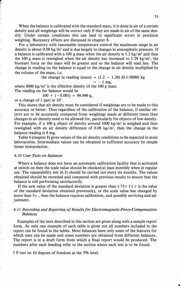
I . l

ij

50

Table 3. Tolerances for Masses

Nominal OIML CLASSIFICATIONS

NML NML

Values Class E 1 Class E2 Class F 1 Class F2 Class M1 Class A Class B

±mg ± mg ± mg ± mg ± mg ± mg ± mg

50 kg 25 75 250 750 2500 500 2500 20 kg 10 30 100 300 1000 200 1000 10 kg 5 15 50 150 500 100 500 5 kg 2.5 7.5 25 75 250 50 250 2 kg 1.0 3.0 10 30 100 20 100 1 kg 0.50 1.5 5 15 50 10 50

500 g 0.25 0.75 2.5 7.5 25 5 25 200 g 0.10 0.30 1.0 3.0 10 2.0 10 100 g 0.05 0.15 0.5 1.5 5 1.0 5 50 g 0.030 0.010 0.30 1.0 3.0 0.5 2.5 20 g 0.025 0.080 0.25 0.8 2.5 0.2 1.0 10 g 0.020 0.060 0.20 0.6 2.0 0.10 0.5 5 g 0.015 0.050 0.15 0.5 1.5 0.10 0.5 2 g 0.012 0.040 0.12 0.4 1.2 0.10 0.5 1 g 0.010 0.030 0.10 0.3 1.0 0.10 0.5

500 mg 0.008 0.025 0.08 0.25 0.8 0.10 0.5 200 mg 0.006 0.020 0.06 0.20 0.6 0.10 0.5 100 mg 0.005 0.015 0.05 0.15 0.5 0.10 0.5 50 mg 0.004 0.012 0.04 0.12 0.4 0.05 0.2 20 mg 0.003 0.010 0.03 0.10 0.3 0.05 0.2 10 mg 0.002 0.008 0.025 0.08 0.25 0.05 0.2

5 mg 0:002 0.006 0.020 0.06 0.20 0.05 0.2 2 mg 0.002 0.006 0.020 0.06 0.20 0.05 0.2 1 mg 0.002 0.006 0.020 0.06 0.20 0.05 0.2

6.8.2 Built-in calibration mass A built-in calibration mass is usually well protected and unlikely to change

significantly unless the balance is in a harsh environment. However it should be checked at least every one or two years, depending upon use and environment. This is done by calibrating the balance using the procedure nominated by the manufac­turer and then weighing a standard mass of nominal value equal to either the calibra­tion mass or the maximum capacity if the value of the calibration mass is unknown. If the value of the built-in calibration mass is correct then the balance will display the value of the standard mass. Any standard masses that are used must have an uncertainty of calibration of no more than half the discrimination of the balance (i.e. if the discrimination is 1 mg the standard mass should have an uncertainty of calibration no larger than ± 0.5 mg), but its actual value is unimportant as this can be allowed for by calculation.

6.9 Air Buoyancy and Weighing

Unlike other balances there is no direct compensation for buoyancy, as with single-pan substitution balances, or two-pan balances where the buoyancy of the ob­ject is effectively balanced against that of stainless-steel standards.

51

When the balance is calibrated with the standard mass, it is done in air of a certain density and all weighings will be correct only if they are made in air of the same den­sity. Under certain conditions this can lead to significant errors in precision weighing. Buoyancy effects are discussed in chapter 8.

For a laboratory with reasonable temperature control the maximum range in air density is about 0.08 kg/m3 and is due largely to changes in atmospheric pressure. If a balance is calibrated with a 100 g mass when the air density is 1.2 kg/m3 and then the 100 g mass is reweighed when the air density has increased to 1.28 kg/m3

, the buoyant force on the mass will be greater and so the balance will read less. The change in reading on the balance is equal to the change in air density multiplied by the volume of the mass, i.e.

the change in reading (mass) = (1.2 - 1.28) (0.1 /8000) kg = -1 mg,

where 8000 kg/m3 is the effective density of the 100 g mass. The reading on the balance would be

100 + (-0.001) = 99.999 g, or a change of 1 part in 105

•

This shows that air density must be considered if weighings are to be made to this accuracy or better. Thus regardless of the calibration of the balance, if similar ob­jects are to be accurately compared from weighings made at different times then changes in air density need to be allowed for, particularly for objects of low density. For example, if a 100 g object of density around 1000 kg/m3 is weighed and then reweighed with an air density difference of 0.08 kg/m3, then the change in the balance reading is 8 mg.

Table 4 (chapter 8) gives values of the air density conditions to be expected in most laboratories. Intermediate values can be obtained to sufficient accuracy by simple linear interpolation.

6.10 User Tests on Balances

Where a balance does not have an automatic calibration facility that is activated at switch-on then the scale value should be checked at least monthly when in regular use. The repeatability test (6.3) should be carried out every six months. The values obtained should be recorded and compared with previous results to ensure that the balance is still performing satisfactorily.

If the new value of the standard deviation is greater than 1. 73 a- t ( a- is the value of the standard deviation obtained previously), or the scale value has changed by more than 3 a- , then the balance requires calibration, and possibly servicing and ad­justment.

6.11 Recording and Reporting of Results for Electromagnetic-Force-Compensation Balances

Examples of the tests described in this section are given along with a sample report · form. As only one example of each table is given not all numbers included in the

report can be found in the tables. Most balances have only some of the features forwhich tests can be made and some numbers are obtained from different balances.The report is in a draft form from which a final report would be produced. Thenumbers after each heading refer to the section where each test is to be found.

t F-test on 10 degrees of freedom at the 5% level.

' ,

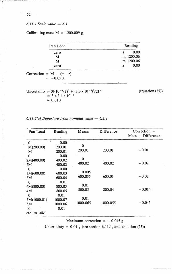
52

6. 11.1 Scale value - 6.1

Calibrating mass M = 1200.009 g

Pan Load

zero M M

zero

Correction = M - (m -z) = -0.05 g

Uncertainty= 3[(10- 3/3)2 + (3.3 x 10- 3) 2/2] v,= 3 x 2.4 x 10- 3

= 0.01 g

6. ll.2(a) Departure from nominal value - 6.2.1

Pan Load Reading Means Difference

0 0.00 M(200.00) 200.01 M 200.01

0 200.01 200.01

0 0.00 2M(400.00) 400.02 2M 400.02

0 400.02 400.02

0 0.00 3M(600.00) 600.03 3M 600.04

0.005 600.035 600.03

0 0.01 4M(800.00) 800.05 4M 800.05

0.01 800.05 800.04

0 0.01 5M(1000.0l) 1000.07 SM 1000.06

0.01 1000.065 1000.055

0 0.01 etc. to lOM

Reading

z 0.00 m 1200.06 m 1200.06 z 0.00

(equation (25))

Correction = Mass - Difference

-0.01

-0.02

-0.03

-0.014

-0.045

Maximum correction = -0.045 g

Uncertainty = 0.01 g (see section 6.11.1, and equation (25))

53

6. ll .2(b) Departure from nominal value - 6.2.2

Calibrating Mass M = 200.00 g Note: M' = M

Pan Reading Means Difference Correction Cumulative Load M - difference Correction

0 0.00 M 200.01 0.00

M 200.01 200.01 -0.01 -0.010 0.00 200.01

M' 200.01 M' + M 400.02 200.015

M' + M 400.03 200.01 -0.01 -0.02M' 200.02 400.025

2M' 400.03 2M' + M 600.04 400.03

2M' + M 600.04 200.01 -0.01 -0.032M' 400.03 600.04

3M' 600.00 3M' + M 800.01 600.005

3M' + M 800.02 200.01 -0.01 -0.043M' 600.01 800.015

4M' 800.04 4M' + M 1000.05 800.04

4M' + M 1000.05 200.01 -0.01 -0.054M' 800.04 1000.05

Maximum correction = -0.05 g

Uncertainty - see section 6.11.1

6. 11.2(c) Departure from nominal value - value of the calibrating mass unknown-6.2.2

Different values from those of 6. l l .2(b) are used in this example. M is assumed tobe equal to the first difference = 200.00 g

Difference Correction Cumulative (g) ci Correction

Ki

1 200.00 0 0 2 200.01 -0.01 -0.013 200.01 -0.01 -0.024 200.01 -0.01 -0.035 200.01 -0.01 -0.04

Here R = 1000 g K, = -0.04 g

Uncertainty - see section 6.11.1

i.M.K/R-Ki

-0.008-0.0

-0.016+0.01

-0.024+0.02

-0.032 + 0.03

-0.04 +0.04

Final Correction

(g)

-0.008

-0.006

-0.004

-0.002

0.000

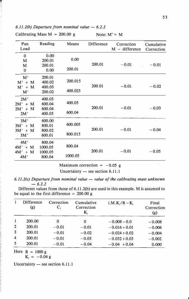
_; __ � ____ : -----,-------�·· . . -- -�--·---·--:- -· ·-.cc -"'- --- -

52

6. 11.1 Scale value - 6.1

Calibrating mass M = 1200.009 g

Pan Load

zero M M

zero

Correction = M - (m -z ) = -0.05 g

Uncertainty;= 3[(10- 3/3)2 + (3.3x 10-3)2/2] Y2

=3x 2.4x 10- 3

""' 0.01 g

6. ll .2(a) Departure from nominal value - 6.2.1

Pan Load Reading Means Difference

0 0.00 M(200.00) 200.01 0

M 200.01 200.01 200.01

0 0.00 2M( 400.00) 400.02 0

2M 400.02 400.02 400.02

0 0.00 3M(600.00) 600.03 0.005

3M 600.04 600.035 600.03

0 0.01 4M( 800.00) 800.05 0.01

4M 800.05 800.05 800.04

0 0.01 5M(1000.0l) 1000.07 0.01

SM 1000.06 1000.065 1000.055

0 0.01 etc. to 10M

Reading

z 0.00 m 1200.06 m 1200.06 z 0.00

(equation ( 25))

Correction = Mass - Difference

-0.01

-0.02

-0.03

-0.014

-0.045

Maximum correction = - 0.045 g

Uncertainty = 0.01 g (see section 6.11.1, and equation ( 25))

·r---

53

6.ll.2(b) Departure from nominal value - 6.2.2

Calibrating Mass M = 200.00 g Note: M'""' M

Pan Reading Means Difference Correction Cumulative Load M -difference Correction

0 0.00 M 200.01 0.00

M 200.01 20·0.01 -0.01 -0.010 0.00 200.01

M' 200.01 M' + M 400.02 200.015

M' + M 400.03 200.01 -0.01 -0.02M' 200.02 400.025

2M' 400.03 2M' + M 600.04 400.03

2M' + M 600.04 200.01 -0.01 ,-0.03 2M' 400.03 600.04

3M' 600.00 3M' + M 800.01 600.005

3M' + M 800.02 200.01 -0.01 -0.043M' 600.01 800.015

4M' 800.04 4M' + M 1000.05 800.04

4M' + M 1000.05 200.01 -0.01 -0.054M' 800.04 1000.05

Maximum correction = -0.05 g

Uncertainty - see section 6.11.1

6.11.2(c) Departure from nominal value - value of the calibrating mass unknown -6.2.2

Different values from those of 6.11.2(b ) are used in this example . M is assumed to be equal to the first difference = 200.00 g

Difference Correction (g) ci

1 200.00 0 2 200.01 -0.013 200.01 -0.014 200.01 -0.015 200.01 -0.01

Here R=lOOOg K, = -0.04 g

Uncertainty - see section 6.11.1

Cumulative Correction

Ki

0 -0.01-0.02-0.03-0.04

i .M .K/R -Ki Final

-0.008-0.0-0.016 + 0.01-0.024+0.02-0.032 + 0.03-0.04 +0.04

Correction (g)

-0.008-0.006-0.004-0.002

0.000

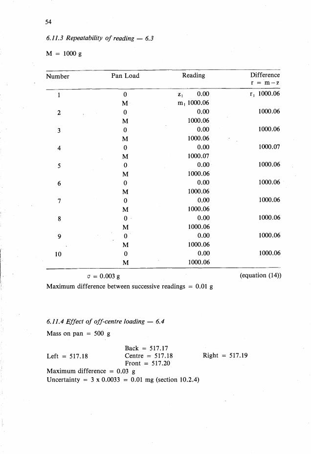
ll

I

I;.

54

6.11.3 Repeatability of reading - 6.3

M = 1000 g

Number Pan Load

1 0

M

2 0

M

3 0

M

4 0

M

5 0

M

6 0

M

7 0

M

8 0

M

9 0

M

10 0

M

Reading Difference r = m-z

Z1 0.00 r 1 1000.06

m 1 1000.06

0.00 1000.06

1000.06

0.00 1000.06

1000.06

0.00 1000.07

1000.07

0.00 1000.06

1000.06

0.00 1000.06

1000.06

0.00 1000.06

1000.06

0.00 1000.06

1000.06

0.00 1000.06

1000.06

0.00 1000.06

1000.06

6.11.5 Hysteresis - 6.5

M (half capacity of balance) = 500 g

Pan Load

Zero Z1 M m1

M + M' M m

2

Zero Zz

1 2

0.00 0.00 500.03 500.03 700.04 700.04 500.03 500.03

0.00 0.00

Hysteresis = M1 - M2 = 0.00 and Z1

- Z2 = 0.00

Uncertainty = 3 x 0.0033/6Vz - = 0.004 g

55

3

0.00 500.03 700.04 500.03

0.00

Note: The factor 1/6Y, occurs because it is effectively double weighing repeated 3

times - see equation (25).

6.11.6 Check of built-in calibration mass - 6.8

Calibrate the balance according to the procedure laid down by the manufacturer. Read the balance with known mass M on the pan. M should be approximately

equal to the built-in calibration mass. Standard mass, M = 1200.009 g Balance reading = m = 1200.01 g

Balance correction = M - m = 1200.01 - 1200.01 = 0.00 g Value of built-in calibration mass = nominal value + correction

= 1200.00 + 0.00 = 1200.00 g

a= 0.003 g (equation (14)) Uncertainty negligible.)

0.01 g (see section 10.2 - uncertainty of the standard mass M is

Maximum difference between successive readings = 0.01 g

6.11.4 Effect of off-centre loading - 6.4

Mass on pan = 500 g

Left = 517.18

Back = 517.17 Centre = 517.18 Front = 517.20

Maximum difference = 0.03 g

Uncertainty = 3 x 0.0033 = 0.01 mg (section 10.2.4)

Right = 517.19

- �-,,,,,,, .... , -""',"f,ff/ ,���- - -- �-------------- ------- ""ff

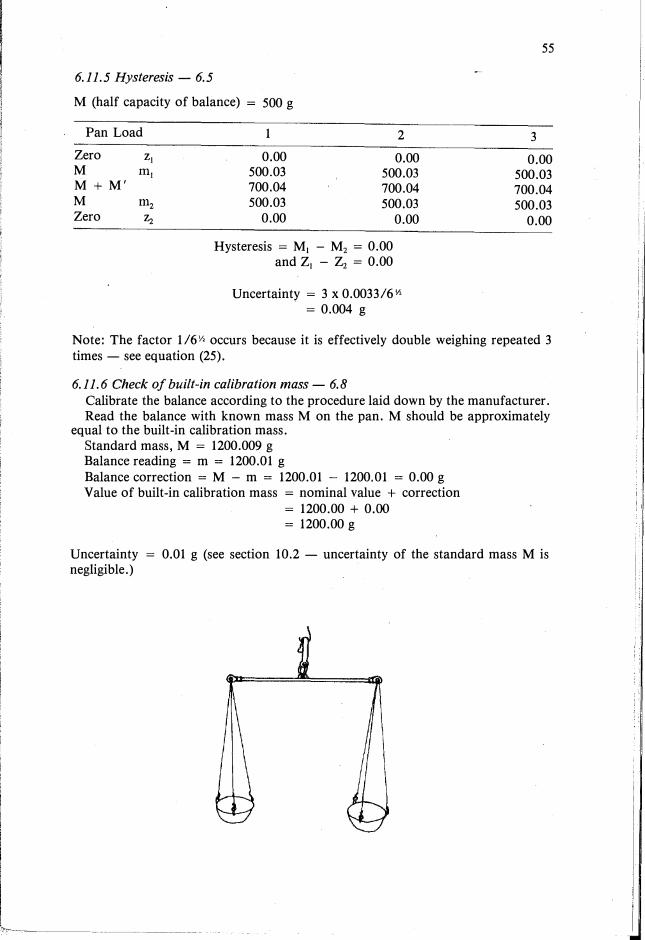
1-r' .,

' Ii

. ii

1: ,,I

'�·-

54

6.11.3 Repeatability ofreading - 6.3

M = 1000 g

Number Pan Load Reading

1 0 Z 1 0.00

M m 1 1000.06

2 0 0.00

M 1000.06

3 0 0.00

M 1000.06

4 0 0.00

M 1000.07

5 0 0.00

M 1000.06

6 0 0.00

M 1000.06

7 0 0.00

M 1000.06

8 0 0.00

M 1000.06

9 0 0.00

M 1000.06

10 0 0.00

M 1000.06

CJ= 0.003 g

Maximum difference between successive readings = 0.01 g

6.11.4 Effect of off-centre loading - 6.4

Mass on pan = 500 g

Difference r = m-z

r 1 1000.06

1000.06

1000.06

1000.07

1000.06

1000.06

1000.06

1000.06

1000.06

1000.06

(equation (14))

Left = 517.18

Back = 517.17 Centre = 517.18 Front = 517.20

Right = 517.19

Maximum difference = 0.03 g

Uncertainty = 3 x 0.0033 = 0.01 mg (section 10.2.4)

6.11.5 Hysteresis - 6.5

M (half capacity of balance) 500 g

Pan Load

Zero Z1 M ill1

M + M'

M ill2Zero Z2

1 2

0.00 0.00 500.03 500.03 700.04 700.04 500.03 500.03

0.00 0.00

Hysteresis = M1 - M2 = 0.00 and Z1 - Z2 = 0.00

Uncertainty = 3 x 0.0033/6 v, . = 0.004 g

55

3

0.00 500.03 700.04 500.03

0.00

Note: The factor 1 /6 Y, occurs because it is effectively double weighing repeated 3

times - see equation (25).

6.11.6 Check of built-in calibration mass - 6.8

Calibrate the balance according to the procedure laid down by the manufacturer. Read the balance with known mass M on the pan. M should be approximately

equal to the built-in calibration mass. Standard mass, M = 1200.009 g Balance reading = m = 1200.01 g

Balance correction = M - m = 1200.01 - 1200.01 = 0.00 g Value of built-in calibration mass = nominal value + correction

= 1200.00 + 0.00 = 1200.00 g

Uncertainty = 0.01 g (see section 10.2 - uncertainty of the standard mass M is negligible.)

: i

56

6.11. 7 Sample Report on electronic balances

REPORT ON SINGLE-PAN ELECTRONIC BALANCE

Maker Mettler Model P 1200 Serial No. 13254 Capacity 1200 g Discrimination (least digit) 0.01 g Type (top-loading or analytical) Top-loading

Client CSIRO Examined at (precise location) Room C20E, National Measurement Laboratory

Temperature of test 20. 4 °C

Repeatability of Reading

Reading (g)

500

1000

Standard Deviation of reading (g)

0.003

0.003

Departure from Nominal Value

Reading

(g)

JOO. 200 300 400 500 600 700 800 900

1000 1100

Off-Centre Loading

Correction

(g)

0.00 -0.01-0.01-0.02-0.02-0.03-0.03-0.04-0.04-0.05-0.05

Maximum difference between successive readings (g)

0.00

0.01

Uncertainty ( ±)

(g)

0.01

A mass of approximately 500 g was placed on a disk of 50 mm diameter and mov­

ed to various positions on the pan. The balance readings obtained are given in the

table.

Centre Front Back

0.00 +0.02 -0.01

Left Right

0.00 +0.01

Maximum difference (g)

0.03

57

Load Hysteresis

500 g less than 0. OJ g

Calibrating Mass

The value of the calibrating mass incorporated in the balance was measured on the basis of weighings made in air of density 1.2 kg/m 3 against masses of density 8000 kg/m3.

Accuracy

Value 1200.00 g Uncertainty = ± 0.01 g

Limit of performance for the balance Uncertainty of weighing of the balance

±0.06 g ± 0.014 g

Uncertainties quoted in this Report have been estimated on the basis of there be­ing not more than one chance in one hundred that any value differs from the true value by more than the stated uncertainty.

Notes

1. The balance has been tested according to the specifications laid down inThe Calibration of Balances

David B. Prowse CSIRO National Measurement Laboratory

Chapter 6.

2. When the sign of the correction is positive (+)the amount should be added to thescale reading to give the correct value and when negative ( - ) subtracted from it.3. Air buoyancy corrections should be calculated on the basis that the object beingweighed is balanced against a hypothetical mass of density 8000 kg/m3 in air ofmeasured density.4. The Limit of Performance is the tolerance band within which all readings of thebalance will fall.

7. Ultra-Microbalances

7.1 Introduction

An ultra-microbalance is a balance with a discrimination of 1 µg or less. These balances operate on the principle of electromagnetic-force compensation but with some form of mechanical taring so that the balance can be operated in the electronic range with relatively large loads. They usually have two or more electronic ranges, of which only the most sensitive has a discrimination of 1 µg or less. The maximum capacity is usually 3 to 5 g.

Unless built-in masses are provided the balance operates very much like a conven­tional two-pan damped balance, but with electronic readout, variable range and

I yr

.;Ii : [I

i i\'1

ii I

\!'

! I' I

56

6.11. 7 Sample Report on electronic balances

REPORT ON SINGLE-PAN ELECTRONIC BALANCE

Maker Mettler Model P 1200 Serial No. 13254

Capacity 1200 g Discrimination (least digit) 0. 01 g

Type (top-loading or analytical) Top-loading

Client CSIRO Examined at (precise location) Room C20E, National Measurement Laboratory

Temperature of test 20. 4 °C

Repeatability of Reading

Reading (g)

500

1000

Standard Deviation of reading (g)

0.003

0.003

Departure from Nominal Value

Reading (g)

100 200

300 400 500 600 700 800

900

1000 1100

Off-Centre Loading

Correction (g)

0.00

-0.01

-0.01-0.02-0.02

-0.03-0.03

-0.04

-0.04

-0.05-0.05

Maximum difference between successive readings (g)

0.00

0.01

Uncertainty ( ±) (g)

0.01

A mass of approximately 500 g was placed on a disk of 50 mm diameter and mov­ed to various positions on the pan. The balance readings obtained are given in the table.

Centre Front Back Left

0.00 +0.02 -0.01 0.00

�---·--- ��-----��---- _ _ ,,_ -- - · · ---

Right

+0.01

Maximum difference (g)

0.03

57

Load Hysteresis 500 g less than 0. 01 g

Calibrating Mass

The value of the calibrating mass incorporated in the balance was measured on the basis of weighings made in air of density 1.-2 kg/m 3 against masses of density 8000 kg/m3.

Accuracy

Value = 1200.00 g Uncertainty = ± 0.01 g

Limit of performance for the balance Uncertainty of weighing of the balance

= ±0.06 g ±0.014 g

Uncertainties quoted in this Report have been estimated on the basis of there be­ing not more than one chance in one hundred that any value differs from the true value by more than the stated uncertainty.

Notes

1. The balance has been tested according to the specifications laid down inThe Calibration of Balances

David B. Prowse CSIRO National Measurement Laboratory

Chapter 6.

2. When the sign of the correction is positive (+)the amount should be added to thescale reading to give the correct value and when negative ( - ) subtracted from it.3. Air buoyancy corrections should be calculated on the basis that the object beingweighed is balanced against a hypothetical mass of density 8000 kg/m3 in air ofmeasured density.4. The Limit of Performance is the tolerance band within which all readings of thebalance will fall.

7. Ultra-Microbalances

7.1 Introduction

An ultra-microbalance is a balance with a discrimination of 1 µg or less. These balances operate on the principle of electromagnetic-force compensation but with some form of mechanical taring so that the balance can be operated in the electronic range _with relatively large loads. They usually have two or more electronic ranges,of which only the most sensitive has a discrimination of 1 µg or less. The maximum capacity is usually 3 to 5 g.

Unless built-in masses are provided the balance operates very much like a conven­tional two-pan damped balance, but with electronic readout, variable range and

IT 'I ii

'!ii 11 !'.

ii I I

!t!'.

58

discrimination. All weighing is done by either direct reading for small loads within the electronic weighing range, or by substitution for heavier loads.

Because of the difficulty of making and calibrating masses smaller than 1 mg the testing of these balances is quite a problem. For balances with a scale range of at least 10 mg, regardless of the resolution, the problem reduces to that of a conven­tional balance. Depending upon the form of the balance, the appropriate tests from chapter 6 can be used. Small masses, calibrated with an uncertainty of 1 µg by the Laboratory, can be used for these tests.

It should be noted that these balances, more than most other types of balance, tend to be used for special purposes and with special equipment. In these cases a conventional calibration is often not wanted nor is it appropriate. Often the user is interested in only one or two features, e.g. resolution and long-term stability.

7.2 Testing of Balances with a Discrimination of 0.1 µg

Calibration of masses with an accuracy of better than 1 µg is very difficult, if not virtually impossible. This effectively limits the calibration of ultra-microbalances to this accuracy. It is possible to do some internal checks to slightly better than this but not to obtain absolute mass values.

Most ultra-microbalances have a calibration mass of 10 or 100 mg which is used to adjust the full-scale value of one range. This range can then be calibrated as described for other balances. The other ranges then derive their calibration from this one by electrical division or multiplication. Within the resolution of each range this can be checked by switching ranges and observing whether the same values are ob­tained. In many cases this will be adequate, but where more information is required the following tests can be carried out. 7.2.1 Repeatability of reading

This can be checked using the methods listed in sections 4.1, 5.1 and 6.3. Whatever method is used it should involve lifting masses off the pan(s). 7.2.2 Scale value

It is possible to calibrate a 1 mg mass to about 1 µg, which effectively limits to this value the calibration of the range with a discrimination of 0.1 µg. An accuracy ap­proaching the discrimination can be obtained by using the balance at a fraction of its range as outlined in section 10.2.2. In this way it can be used to compare masses or objects to an accuracy approaching the repeatability of the balance. Thus, like two­pan, three-knife-edge balances, an ultra-microbalance can be used as a comparator (to accuracies approaching 0.1 µg), but will not measure mass to better than the ac­curacy of the calibration masses (approximately 1 µg).

If the balance is to be used for comparing objects of 1 g or more then the change of scale value, or sensitivity, with load should be measured. 7.2.3 Departure from nominal value

Because of the small range (usually 1 mg for the range with 0.1 µg discrimi­nation), the uniformity can be measured by the following methods. (i) With aluminium sheet a set of mg masses of the following denominations can bemade:

2.0, 2.1, 2.2., 2.3, 2.4, 2.5, 2.5', 2.6, 2.7, 2.8, 2.9, 3.0. The sum of these masses is 30 mg. Schemes for calibrating these masses in terms

of a 30 mg standard give an uncertainty of about 1 f1g. They can then be used to check the uniformity of the scale in 0.1 mg steps. (ii) Aluminium foil can be used to make two equal masses of approximately half the

59

range (e.g. 0.5. mg). These are each weighed on the balance and then weighedtogeth�r. The difference between the sum of the individual values and the combinedvalues is a measure of the uniformity at mid-range. This method is not as comprehensive as (i) but it is quicker and much easier to im­

plement. 7.2.4 Stability

Some ultra-microbalances are used to measure over periods ranging from minutesto days. To know how accurately the property is being measured the change ofreading with time, i.e. the stability, should be determined. The stability should bemeasured with the balance both loaded and unloaded. Care must be taken to allowfor, or eliminate, the effects of air buoyancy and changes in ambient temperature asthese may mask the measurement of the stability. 7.2.5 Damping

Mos: ul�ra-mi�robalances are critically damped or slightly underdamped, but dueto P.a? swmg, air current.s, etc., it can take 30 to 60 seconds for the reading tostabilise. In some cases this period can lengthen considerably for larger loads. Thisc_an be checked b� placing e��al loads of at least 1 g in each pan and measuring thetime for the readmg to stabilise on the range with discrimination of 0.1 µg.

8. Buoyancy Effects

Wh�n an object is weighed in air it experiences an upthrust, or buoyant force (lossof weight), equal to the weight of air displaced. This buoyant force causes manyproblems and much confusion in weighing. It is not practical to weigh in vacuum?ecause of the surface effects that would occur on the objects being weighed. Whatis termed the 'true mass' of an object is the mass that would be measured in avacuum, providing everything else (surface layers, etc.) was unchanged. Thus in ast�ndards laboratory, it is true mass values which are measured in calibratingpnmary standards and all other values are calculated from these (Pontius, 1974;Prowse, 1984).

If the mass is measured on a weighing system (e.g. a spring balance) the value ob-tained would be M ' , here

M'g = (M - dV)g where d is the air density and V is the volume of the mass.

Since g occurs on both sides it can be eliminated from this equation and all equa­tions where masses are directly compared. Therefore

M' = M(l - d/D).

If two objects, denoted by subscripts 1 and 2, are weighed then the difference inmass is given by

(15)

Thus if M1 is know� th.en M2 can be calculated provided that d1 , d2, V1 and V2 arealso ��own. If the weighmgs are done at nearly the same time, and under the same

condit10ns, then d1 = d2, and if the masses are made of the same material then V1 =V 2 so that (15) reduces to

·I

ii ii 11 [i

11

Ii ii

I'

i! Ii ,1

58

discrimination. All weighing is done by either direct reading for small loads within the electronic weighing range, or by substitution for heavier loads.

Because of the difficulty of making and calibrating masses smaller than 1 mg the testing of these balances is quite a problem. For balances with a scale range of at least 10 mg, regardless of the resolution, the problem reduces to that of a conven­tional balance. Depending upon the form of the balance, the appropriate tests from chapter 6 can be used. Small masses, calibrated with an uncertainty of 1 µg by the Laboratory, can be used for these tests.

It should be noted that these balances, more than most other types of balance, tend to be used for special purposes and with special equipment. In these cases a conventional calibration is often not wanted nor is it appropriate. Often the user is interested in only one or two features, e.g. resolution and long-term stability.

7.2 Testing of Balances with a Discrimination of 0.1 µg

Calibration of masses with an accuracy of better than 1 µg is very difficult, if not virtually impossible. This effectively limits the calibration of ultra-microbalances to this accuracy. It is possible to do some internal checks to slightly better than this but not to obtain absolute mass values.

Most ultra-microbalances have a calibration mass of 10 or 100 mg which is used to adjust the full-scale value of one range. This range can then be calibrated as described for other balances. The other ranges then derive their calibration from this one by electrical division or multiplication. Within the resolution of each range this can be checked by switching ranges and observing whether the same values are ob­tained. In many cases this will be adequate, but where more information is required the following tests can be carried out. 7.2.1 Repeatability of reading

This can be checked using the methods listed in sections 4.1, 5.1 and 6.3. Whatever method is used it should involve lifting masses off the pan(s). 7.2.2 Scale value

It is possible to calibrate a 1 mg mass to about 1 µg, which effectively limits to this value the calibration of the range with a discrimination of 0.1 µg. An accuracy ap­proaching the discrimination can be obtained by using the balance at a fraction of its range as outlined in section 10.2.2. In this way it can be used to compare masses or objects to an accuracy approaching the repeatability of the balance. Thus, like two­pan, three-knife-edge balances, an ultra-microbalance can be used as a comparator (to accuracies approaching 0.1 µg}, but will not measure mass to better than the ac­curacy of the calibration masses (approximately 1 µg).

If the balance is to be used for comparing objects of 1 g or more then the change of scale value, or sensitivity, with load should be measured. 7.2.3 Departure from nominal value

Because of the small range (usually 1 mg for the range with 0.1 µg discrimi­nation}, the uniformity can be measured by the following methods. (i) With aluminium sheet a set of mg masses of the following denominations can bemade:

2.0, 2.1, 2.2., 2.3, 2.4, 2.5, 2.5 ', 2.6, 2.7, 2.8, 2.9, 3.0. The sum of these masses is 30 mg. Schemes for calibrating these masses in terms

of a 30 mg standard give an uncertainty of about 1 �1g. They can then be used to check the uniformity of the scale in 0.1 mg steps. (ii) Aluminium foil can be used to make two equal masses of approximately half the

59

range (e.g. 0.5. mg). These are each weighed on the balance and then weighedtogether. The difference between the sum of the individual values and the combinedvalues is a measure of the uniformity at mid-range. This method is not as comprehensive as (i) but it is quicker and much easier to im­plement.

7.2.4 Stability Some ultra-microbalances are used to measure over periods ranging from minutesto d�ys. To know how accurately the property is being measured the change ofreadmg with time, i.e. the stability, should be determined. The stability should bemeasured with the balance both loaded and unloaded. Care must be taken to allowfor, or eliminate, the effects of air buoyancy and changes in ambient temperature asthese may mask the measurement of the stability.

7.2.5 Damping Most ul�ra-mi�robalances are critically damped or slightly underdamped, but dueto P.a!1 · swmg, air currents, etc., it can take 30 to 60 seconds for the reading tostabilise. In some cases this period can lengthen considerably for larger loads. Thisc:in be checked by placing equal loads of at least 1 g in each pan and measuring thetime for the reading to stabilise on the range with discrimination of 0.1 µg.

8. Buoyancy Effects

Wh�n an object is weighed in air it experiences an upthrust, or buoyant force (loss of weight), equal to the weight of air displaced. This buoyant force causes many problems and much confusion in weighing. It is not practical to weigh in vacuum ?ecause of the surface effects that would occur on the objects being weighed. What is termed the 'true mass' of an object is the mass that would be measured in a vacuum, providing everything else (surface layers, etc.) was unchanged. Thus in a st�ndards laboratory, it is true mass values which are measured in calibrating pnmary standards and all other values are calculated from these (Pontius, 1974; Prowse, 1984).

_If the mass is measured on a weighing system (e.g. a spring bahmce) the value ob­tamed would be M ' , here

M'g = (M - dV)g where d is the air density and V is the volume of the mass.

Since g occurs on both sides it can be eliminated from this equation and all equa­tions where masses are directly compared. Therefore

M' = M(l - d/D).

If two objects, denoted by subscripts 1 and 2, are weighed then the difference in mass is given by

(15)

Thus if M1 is know� th_en M2 can be calculated provided that di , d2, V1 and V2 are also known. If the weighmgs are done at nearly the same time and under the same conditions, then d1 = d2, and if the masses are made of the sa�e material then V1 ""' V 2 so that (15) reduces to

60

This is the case which is normally encountered in the calibration of masses. When

comparing objects made from differing materials, V 1 =I= V 2, and the effect of air

buoyancy must be calculated, or be sufficiently small that it can be neglected for the

accuracy required. When air buoyancy is neglected the value obtained is said to be the mass (weight)

in air of the object, sometimes called apparent mass. This is the value of the masses

. (usually stainless steel) required to balance the object in air of nominal density 1.2

kg/m 3. Consider as an example the weighing of a quantity of water Mw that balances

a stainless-steel mass M ss of density 8000 kg/m 3.

If d = 1.2 kg/m3 then

Mw (1 - 1.2/1000) = M,, (1 - 1.2/8000).

Hence Mw = (1.00105) M,, kg.

This means that if the stainless-steel mass balanced against the water is 1 kg, then

because of the upthrust due to the air, the mass of water balancing the stainless steel

is approximately 1.001 kg, i.e. a difference of 1 g in 1000 g. In this case the true

mass differs from the mass in air by 1 g.

Because the density of the material used for masses changes from one set to

another, the idea of an apparent mass value has arisen. The apparent mass, Ma, is

the amount of any specified material which will balance the unknown in a specified

atmosphere, d0 = 1.2 kg/m3, at the specified temperature of 20°C. For an object

with a true mass M, made from material of density Dm, the calculated apparent mass

value is (16)

where Da is the assumed or apparent density of the material of the masses. The inter­nationally accepted value for Da is 8000 kg/m3 or 8.0 g/cm3, at 20°c. This is com­monly ca}led the 8.0 basis. In Australia the CSIRO National Measurement Laboratory calibrates all masses on this basis.

To convert from a true mass basis to the 8.0 basis using equation (16), we calculate

Ms.o = M[l - 1.2/DmJ/[l - 1.2/8000].

For stainless steel of density 7800 kg/m 3, equation (17) gives

M8 .0 = (0.999 996 15)M.

(17)

When brass was used extensively for standard masses the mass basis was 8.4. Equation (16) gives the conversion from the 8.0 to the 8.4 basis

Ms.4 = M 8 .0[1 - 1.2/8000]/[1 - 1.2/8390.9]

= (0.999 993 Ol)Ms.o

where the density of brass is 8390.9 kg/m3 at 20°C, and is 8400 kg/m3 at 0°C. Thus in high precision weighing, air buoyancy corrections should be calculated on

the basis that the density of the masses is 8000 kg/m3 and the actual value of the den­sity of the air in the balance case, or room, should be used.

A table of density values for the conditions likely to be encountered in most laboratories is given in Table 4, based on the formula recommended by the BIPM (Giacomo, 1982). Intermediate values may be obtained to sufficient accuracy by linear interpolation.

Table 4. Air Density kg/m3 (1 kg/m3 = 0.001 g/cm3)

Temperature Relative humidity oc 30% 50% 70%

Pressure = 740 mmHg = 986 59 Pa 10 1.212 63 1.211 49 1.210 35 15 1.190 87 1.189 32 1.187 76 20 1.169 65 1.167 56 1.165 46 25 1.148 88 1.146 09 1.143 31

30 1.128 48 1.124 81 1.121 14 35 1.108 36 1.103 57 1.098 79 40 1.088 41 1.082 23 1.076 07 45 1.068 53 1.060 63 1.052 75

Pressure = 750 mmHg = 999 92 Pa 10 1.229 05 1.227 91 1.226 77 15 1.207 01 1.205 45 1.203 90 20 1.185 51 1.183 41 1.181 32 25 1.164 47 1.161 68 1.158 90

30 1.143 81 1.140 14 1.13647 35 1.123 44 1.118 65 1.113 87 40 1.103 25 1.097 07 1.090 90 45 1.083 13 1.075 23 1.067 35

Pressure = 760 mmHg = 1013 25 Pa 10 1.245 47 1.244 33 1.243 19 15 1.223 13 1.221 58 1.220 03 20 1.201 36 1.199 26 1.197 17 25 1.180 06 1.177 27 1.174 48

30 1.159 14 1.155 47 1.151 80 35 1.138 52 1.133 73 1.128 95 40 1.118 09 1.111 91 1.105 74 45 1.097 74 1.089 83 1.081 95

Pressure = 770 mmHg = 1026 58 Pa 10 1.261 88 1.260 75 1.259 61 15 1.239 26 1.237 71 1.236 16 20 1.217 21 1.215 12 1.213 02 25 1.195 64 1.192 85 1.190 07

30 1.174 47 1.170 80 1.167 13 35 1.153 60 1.148 81 1.144 03 40 1.132 92 1.126 74 1.120 58 45 1.112 34 1.104 44 1.096 56

61

900/o

1.209 22 1.186 21 1.163 37 1.140 53

1.117 48 1.094 02 1.069 91 1.044 89

1.225 63 1.202 34 1.179 23 1.156 11

1.132 81 1.109 10 1.084 75 1.059 49

1.242 05 1.218 48 1.195 08 1.171 70

1.148 14 1.124 18 1.099 59 1.074 10

1.258 47 1.234 61 1.210 94 1.187 29

1.163 47 1.139 26 1.114 43 ! I

!

1.088 70

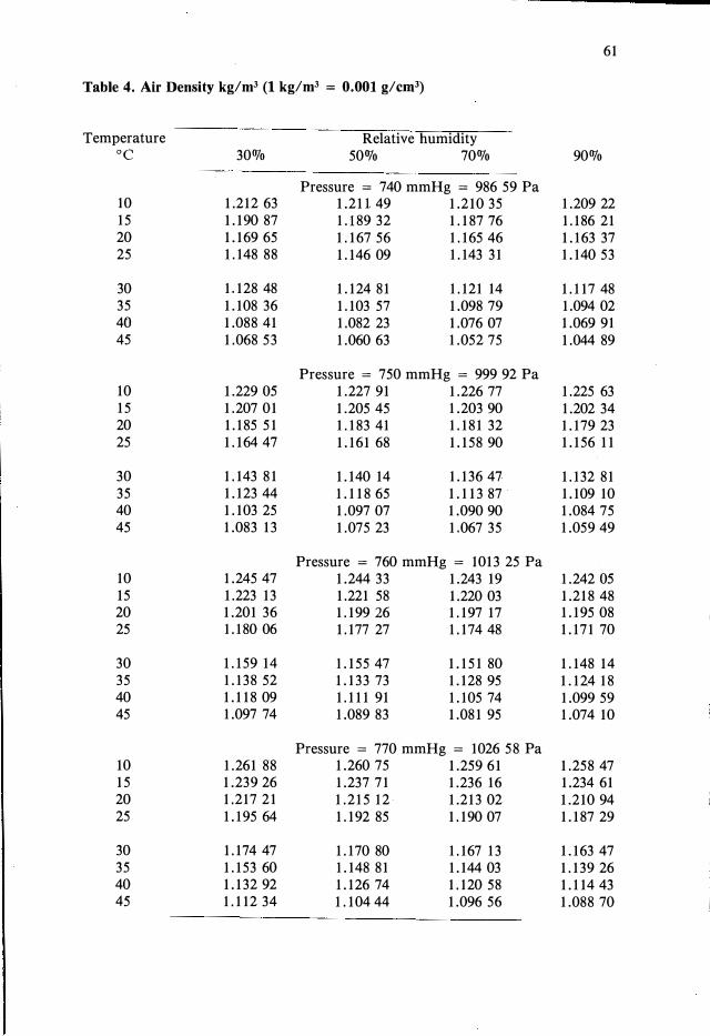
60

This is the case which is normally encountered in the calibration of masses. When

comparing objects made from differing materials, V 1 i= V 2, and the effect of air

buoyancy must be calculated, or be sufficiently small that it can be neglected for the

accuracy required. When air buoyancy is neglected the value obtained is said to be the mass (weight)

in air of the object, sometimes called apparent mass. This is the value of the masses

. (usually stainless steel) required to balance the object in air of nominal density 1.2

kg/m 3• Consider as an example the weighing of a quantity of water Mw that balances

a stainless-steel mass M,, of density 8000 kg/m 3•

If d = 1.2 kg/m3 then

Mw (1 - 1.2/1000) = M,, (1 - 1.2/8000).

Hence Mw = (1.00105) M,, kg. This means that if the stainless-steel mass balanced against the water is 1 kg, then

because of the upthrust due to the air, the mass of water balancing the stainless steel is approximately 1.001 kg, i.e. a difference of 1 g in 1000 g. In this case the true mass differs from the mass in air by 1 g.

Because the density of the material used for masses changes from one set to another, the idea of an apparent mass value has arisen. The apparent mass, Ma, is the amount of any specified material which will balance the unknown in a specified atmosphere, d0 = 1.2 kg/m3

, at the specified temperature of 20°C. For an object with a true mass M, made from material of density D

m, the calculated apparent mass

value is

(16)

where Da is the assumed or apparent density of the material of the masses. The inter­nationally accepted value for Da is 8000 kg/m3 or 8.0 g/cm3, at 20°C. This is com­monly called the 8.0 basis. In Australia the CSIRO National Measurement Laboratory calibrates all masses on this basis.

To convert from a true mass basis to. the 8.0 basis using equation (16), we calculate

Ms.o = M[l - 1.2/DmJ/[l - 1.2/8000].

For stainless steel of density 7800 kg/m3, equation (17) gives

M8.0 = (0.999 996 15)M.

(17)

When brass was used extensively for standard masses the mass basis was 8.4. Equation (16) gives the conversion from the 8.0 to the 8.4 basis

Ms.4 = M8 .0[1 - 1.2/8000]/[l - 1.2/8390.9]

= (0.999 993 Ol)M 8.0

where the density of brass is 8390.9 kg/m3 at 20°C, and is 8400 kg/m3 at 0°C. Thus in high precision weighing, air buoyancy corrections should be calculated on

the basis that the density of the masses is 8000 kg/m3 and the actual value of the den­sity of the air in the balance case, or room, should be used.

A table of density values for the conditions likely to be encountered in most laboratories is given in Table 4, based on the formula recommended by the BIPM (Giacomo, 1982). Intermediate values may be obtained to sufficient accuracy by linear interpolation.

1 Table 4. Air Density kg/m3 (1 kg/m3

= 0.001 g/ cmJ)

Temperature Relative humidity oc 30% 50% 70%

Pressure = 740 mmHg = 986 59 Pa 10 1.212 63 1.211. 49 1.210 35 15 1.190 87 1.189 32 1.187 76 20 1.169 65 1.167 56 1.165 46 25 1.148 88 1.146 09 1.143 31

30 1.128 48 1.124 81 1.121 14 35 1.108 36 1.103 57 1.098 79 40 1.088 41 1.082 23 1.076 07 45 1.068 53 1.060 63 1.052 75

Pressure = 750 mmHg = 999 92 Pa 10 1.229 05 1.227 91 1.226 77 15 1.207 01 1.205 45 1.203 90 20 1.185 51 1.183 41 1.181 32 25 1.164 47 1.161 68 1.158 90

30 1.143 81 1.140 14 1.136 47 35 1.123 44 1.118 65 1.113 87 40 1.103 25 1.097 07 1.090 90 45 1.083 13 1.075 23 1.067 35

Pressure = 760 mmHg = 1013 25 Pa 10 1.245 47 1.244 33 1.243 19 15 1.223 13 1.221 58 1.220 03 20 1.201 36 1.199 26 1.197 17 25 1.180 06 1.177 27 1.174 48

30 1.159 14 1.155 47 1.151 80 35 1.138 52 1.133 73 1.128 95 40 1.118 09 1.111 91 1.105 74 45 1.097 74 1.089 83 1.081 95

Pressure = 770 mmHg = 1026 58 Pa 10 1.261 88 1.260 75 1.259 61 15 1.239 26 1.237 71 1.236 16 20 1.217 21 1.215 12 1.213 02 25 1.195 64 1.192 85 1.190 07

30 1.174 47 1.170 80 1.167 13 35 1.153 60 1.148 81 1.144 03 40 1.132 92 1.126 74 1.120 58 45 1.112 34 1.104 44 1.096 56

61

90%

1.209 22 1.186 21 1.163 37 1.140 53

1.117 48 1.094 02 1.069 91 1.044 89

1.225 63 1.202 34 1.179 23 1.156 11

1.132 81 1.109 10 1.084 75 1.059 49

1.242 05

1.218 48 1.195 08 1.171 70

1.148 14 1.124 18 1.099 59 1.074 10

1.258 47 1.234 61 1.210 94 1.187 29

1.163 47 1.139 26 1.114 43 1.088 70

ii,'

' ' I 'i 1

I···

., I i

62

9. Least-Squares Calibration of Masses Installed in Balances

9.1 Outline and Theory

This chapter describes the application of the method of ieast squar�s to the

analysis of the calibration of the masses installed in the balance (Humphries, 1960;

Bell, 1955). The analysis starts where the other methods finish - it takes the values

· obtained in a direct calibration (section 5.8.2) and analyses them to give the 'best'

values (in the least-squares sense). The calculations are relatively involved but ea� b_e

performed with little difficulty on a modern desk-top computer. From the analys_1s it

is possible to calculate the uncertainty for each dial setting. Because the combma­

tions of masses differ for different balances it is not possible to give a completely

general treatment, but an example can be used to describe the method in sufficient

detail to cover all cases.

Consider a balance that has been calibrated by the method given in section 5.8.2.

Let the actual values for the dial settings for a particular decade be (1), (2), ... (9), and

let A B C D be the actual masses in the balance. The nominal values of A, B, C, ' ' and D are such that

A: B: C: D = 1 : 1 : 2 : 5.

These values, and the equations given in (18), will be different for various combina­

tions of the masses in different balances.

The mass loading arrangement is such that nine equations in the four unknowns

A, B, C and D can be written as follows:

A A + B A + CA + B + C

= (1) = (2) = (3) = (4)

D = (5)B + D = (6)

A + B + D = (7) B + C + D = (8)

A + B + C + D = (9).

(18)

Here the values (1) to (9) are obtained from the calibration described in section

5.8.2, and they may be either corrections to the dial settings, or the actual values of

the dial setting. Let S = [A-(1)]2 + [A+B-(2)]2 + [A+C-(3)]2 + [A+B+C-(4)]2

+ [D-(5)]2 + [B+D-(6)]2 + [A+B+D-(7)]2 + [B+C+D-(8)]2

+ [A+B+C+D-(9)]2. (19)

The principle of least squares states that for S to be a minimum

dS dA

dS dB

dS dC

dS dD o. (20)

Differentiation of (19) gives

6A + 4B + 3C + 2D (1) + (2) + (3) + (4) + (7) + (9)4A + 6B + 3C + 4D = (2) + (4) + (6) + (7) + (8) + (9) 3A + 3B + 4C + 2D = (3) + (4) + (8) + (9) 2A + 4B + 2C + 5D = (5) + (6) + (7) + (8) + (9).

63

(21)

Equations (21) are often called the normal equations. They are four equations in four unknowns and may be solved by many standard methods to give values of A, B, C and D which are denoted by A', B ', C' and D'. These are the least-squares values (or corrections) of the masses in the balance. An analytical solution of equa­tions (19) can be obtained for each combination of built-in masses, but it is easier to use a small computer and one of the least-squares software packages available.

To obtain the value of the dial readings the values A' , B', C', and D' are substituted back into equations (18) to give the final adjusted values of the readings (1)', (2)' , ... (9)' i.e.

A' + B' + C' + D' = (9)', etc.

The residuals (sJ are obtained by subtracting these values from the original values,

S 1 = (l)-(1)',S2 = (2)-(2)', ... S9= (9)-(9)'.

These values should all be about the same order of magnitude. If one is dispropor­tionately larger than the others (e.g. by a factor of three or more) then there is most likely an error in either the measurements or the calculations for that dial setting.

The sum of squares of the residuals (S) is calculated by

If this value is divided by the number of dial settings minus the number of masses (i.e. 9 -4 = 5) then the observational variance is obtained. This is a measure of the uncertainty of the calibration of the masses. From this value it is possible to calculate the uncertainty of each of the dial settings, but because the masses are not used an equal number of times the uncertainties of the dial settings are not equal. However as the differences are not large the standard deviation of each dial setting can be estimated to sufficient accuracy by

0"1 = 2/3 [S/(9 -4)] 112• (22)

Here the "2/3" is a factor inserted to approximate the more rigorous calculation. To obtain the actual uncertainty o-1 must be combined with the uncertainty of the

masses used in the calibration. This is difficult to do rigorously, but a reasonable ap­proximation is to calculate the standard deviation, cr2, of the masses used for each dial combination (see 10.1.3), and then combine it with o-

1 using

(23)

If 0-1 > 40-2, then o-2 may be ignored. The largest value of a should be chosen as the uncertainty for the decade. This will almost certainly occur at dial setting '9', so that only one value need be calculated.

This procedure is repeated for all the decades of the balance.

Ii

I

!· :i

62

9. Least-Squares Calibration of Masses Installed in Balances

9.1 Outline and Theory

This chapter describes the application of the method of ieast squar�s to the

analysis of the calibration of the masses installed in the balance (Humphnes, 1960;

Bell, 1955). The analysis starts where the other methods finish - it takes the values

· obtained in a direct calibration (section 5.8.2) and analyses them to give the 'best'

values (in the least-squares sense). The calculations are relatively involved but ea� b_e

performed with little difficulty on a modern desk-top computer. From the analy�1s 1t

is possible to calculate the uncertainty for each dial setting. Because the combma­

tions of masses differ for different balances it is not possible to give a completely

general treatment, but an example can be used to describe the method in sufficient

detail to cover all cases.

Consider a balance that has been calibrated by the method given in section 5.8.2.

Let the actual values for the dial settings for a particular decade be (1), (2), ... (9), and

let A B C D be the actual masses in the balance. The nominal values of A, B, C' ' '

and D are such that

A: B : C : D = 1 : 1 : 2: 5.

These values, and the equations given in (18), will be different for various combina­tions of the masses in different balances.

The mass loading arrangement is such that nine equations in the four unknowns A, B, C and D can be written as follows:

A (1) A+B (2) A + C (3) A+B + C = (4)

D = (5) (18)

B + D = (6) A+B + D = (7)

B + C + D = (8) A + B + C + D = (9).

Here the values (1) to (9) are obtained from the calibration described in section

5.8.2, and they may be either corrections to the dial settings, or the actual values of

the dial setting. Let S = [A-(1)]2 + [A+B-(2)]2 + [A+C-(3)]2 + [A+B+C-(4)]2

+ [D-(5)]2 + [B + D-(6)]2 + [A +B +D-(7)]2 + [B +C +D-(8)]2

+ [A+B+C+D-(9)]2. (19)

The principle of least squares states that for S to be a minimum

dS dA

� dB

dS dC

dS dD 0. (20)

Differentiation of (19) gives

6A + 4B + 3C + 2D = (1) + (2) + (3) + (4) + (7) + (9) 4A + 6B + 3C + 4D = (2) + (4) + (6) + (7) + (8) + (9) 3A + 3B + 4C + 2D = (3) + (4) + (8) + (9) 2A + 4B + 2C + 5D = (5) + (6) + (7) + (8) + (9).

63

(21)

Equations (21) are often called the normal equations. They are four equations in four unknowns and may be solved by many standard methods to give values of A, B, C and D which are denoted by A', B', C' and D'. These are the least-squares values (or corrections) of the masses in the balance. An analytical solution of equa­tions (19) can be obtained for each combination of built-in masses, but it is easier to use a small computer and one of the least-squares software packages available.

To obtain the value of the dial readings the values A', B', C', and D' are substituted back into equations (18) to give the final adjusted values of the readings (1) I> (2) I , ... (9) I i.e,

A' + B' + C' + D' = (9)', etc.

The residuals (si) are obtained by subtracting these values from the original values,

S1 = (1)-(1)', S2 = (2)-(2)', ... S9 = (9)-(9)'.

These values should all be about the same order of magnitude. If one is dispropor­tionately larger than the others (e.g. by a factor of three or more) then there is most likely an error in either the measurements or the calculations for that dial setting.

The sum of squares of the residuals (S) is calculated by

S = s/ + s/ + ... + si.

If this value is divided by the number of dial settings minus the number of masses (i.e. 9 -4 = 5) then the observational variance is obtained. This is a measure of the uncertainty of the calibration of the masses. From this value it is possible to calculate the uncertainty of each of the dial settings, but because the masses are not used an equal number of times the uncertainties of the dial settings are not equal. However as the differences are not large the standard deviation of each dial setting can be estimated to sufficient accuracy by

cr1 = 2/3 [S/(9-4)P". (22)

Here the "2/3" is a factor inserted to approximate the more rigorous calculation.

To obtain the actual uncertainty cr1 must be combined with the uncertainty of the masses used in the calibration. This is difficult to do rigorously, but a reasonable ap­proximation is to calculate the standard deviation, cr2, of the masses used for each dial combination (see 10.1.3), and then combine it with cr1 using

(23)

If cr1 > 4cr2, then cr2 may be ignored. The largest value of rr should be chosen as the uncertainty for the decade. This will almost certainly occur at dial setting '9', so that only one value need be calculated.

This procedure is repeated for all the decades of the balance.

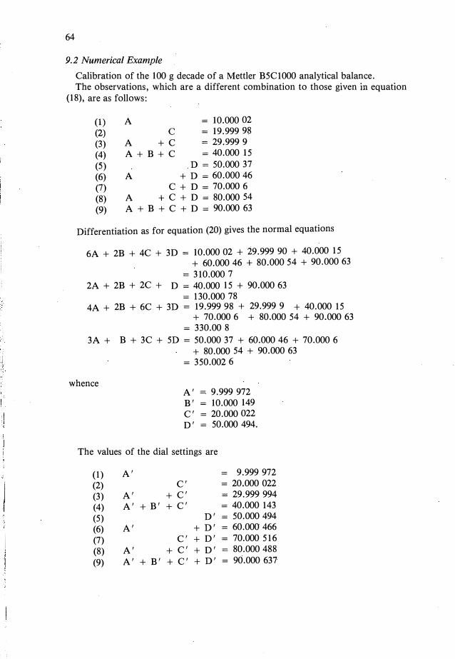
I:· .. 1 ··

il !1i]

t!

64

9.2 Numerical Example

Calibration of the 100 g decade of a Mettler B5C1000 analytical .bala�ce. . The observations, which are a different combination to those given m equation (18), are as follows:

(1)

(2)

(3) (4) (5) (6) (7) (8) (9)

A C

A +C A+B+C

= 10.000 02 = 19.999 98 = 29.999 9 = 40.000 15

A D = 50.000 37

+ D = 60.000 46 C + D = 70.000 6

A + C + D = 80.000 54A + B + C + D = 90.000 63

Differentiation as for equation (20) gives the normal equations

6A + 2B + 4C + 3D = 10.000 02 + 29.999 90 + 40.000 15+ 60.000 46 + 80.000 54 + 90.000 63

= 310.000 7 2A + 2B + 2C + D = 40.000 15 + 90.000 63

= 130.000 78 4A + 2B + 6C + 3D = 19.999 98 + 29.999 9 + 40.000 15

+ 70.000 6 + 80.000 54 + 90.000 63= 330.00 8

3A + B + 3C + 5D = 50.000 37 + 60.000 46 + 70.000 6 + 80.000 54 + 90.000 63

= 350.002 6

whence A' = 9.999 972 B' = 10.000 149 C' = 20.000 022 D' = 50.000 494.

The values of the dial settings are

(1) A' = 9.999 972 (2) C' = 20.000 022 (3) A' + C' = 29.999 994 (4) A' + B' + C' = 40.000 143 (5) D' = 50.000 494 (6) A' + D' = 60.000 466(7) C' + D' = 70.000 516 (8) A' + C' + D' = 80.000 488 (9) A' + B' + C' + D' = 90.000 637

65

Substituting the values for A', B', C', D' back into the original equations gives the residuals

S 1 = 10.000 02 - 9.999 972 = 0.000 048

S2 = 19.999 98 - 20.000 022 = -0.000 042

S3 = 29.999 9 - (9.999 972 + 20.000 022) = -0.000 094

S4 = 40.000 15 - (9.999 972 + 10.000 149 + 20.000 022) = 0.000 007

S5 = 50.000 37 - 50.000 494 = -0.000 124

S6 = 60.000 46 - (9.999 972 + 50.000 494) = -0.000 006

S7 = 70.000 6 - (20.000 022 + 50.000 494) = 0.000 084

Ss = 80.000 54 - (9.999 972 + 20.000 022 + 50.000 494) = 0.000 052

S9 = 90.000 63 - (9.999 972 + 10.000 149 + 20.000 022 + 50.000 494) = -0.000 007

The sum of squares of residuals, S, is given by S = (0.000 048)2 + ( -0.000 042)2 + etc.

= 3.82 X 10-B g2•

Thus u i2 = 213 [S/(9-4)] = 2/3 [3.82 X 10- 8/5],

and u1 = 0.000 058 g.

The uncertainty (30z) of the calibrating masses is 50 g - 50 µg 20 g - 20 µg 10 g - 10 µg.

For the masses used in the calibration of the dials the standard deviations are com­bined according to equation (24). Combining the largest value (dial (9) - 56/3 �tg) with Oj calculated above gives the maximum standard deviation.

Therefore the maximum standard deviation of the dial values is CJ= [u1

2 + uz2F" = [0.000 0582 + 0.000 0192]Vz= 0.000 061 g.

Thus the uncertainty of the dial values for the 10 to 100 g decade is 3 x 0.000 061 g = 0.000 19 g.

10. Estimation of Uncertainty

The aim of this chapter is to enable calibrators, and users, to estimate how ac­curately the calibration has been carried out. It provides a straightforward approach without recourse to statistics, and is aimed to give a guide for assessing the uncer­tainty to be included in reports on the calibration of balances and masses. The for­mulae and methods described are not derived here but may in general be obtained from statistical textbooks.

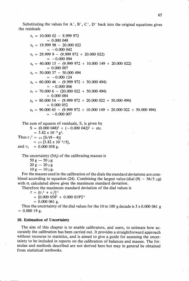
i

1}

!j·J

64

9.2 Numerical Example

Calibration of the 100 g decade of a Mettler B5Cl000 analytical ?ala�ce. . The observations, which are a different combination to those given m equation

(18), are as follows:

(1)

(2) (3) (4) (5) (6) (7) (8) (9)

A C

A +CA+B+C

= 10.000 02 = 19.999 98 = 29.999 9 = 40.000 15

D = 50.000 37 A + D = 60.000 46

C + D = 70.000 6 A + C + D = 80.000 54 A + B + C + D = 90.000 63

Differentiation as for equation (20) gives the normal equations

6A + 2B + 4C + 3D = 10.000 02 + 29.999 90 + 40.000 15 + 60.000 46 + 80.000 54 + 90.000 63

= 310.000 7 2A + 2B + 2C + D = 40.000 15 + 90.000 63

= 130.000 78 4A + 2B + 6C + 3D = 19.999 98 + 29.999 9 + 40.000 15

+ .70.000 6 + 80.000 54 + 90.000 63 = 330.00 8

3A + B + 3C + 5D = 50.000 37 + 60.000 46 + 70.000 6 + 80.000 54 + 90.000 63

= 350.002 6

whence A' = 9.999 972 B' = 10.000 149 C' = 20.000 022 D' = 50.000 494.

The values of the dial settings are

(1) A' = 9.999 972 (2) C' = 20.000 022 (3) A' + C' = 29.999 994 (4) A' + B' + C' = 40.000 143 (5) D' = 50.000 494 (6) A' + D' = 60.000 466 (7) C' + D' = 70.000 516 (8) A' + C' + D' = 80.000 488 (9) A' + B' + C' + D' = 90.000 637

65

Substituting the values for A', B', C', D' back into the original equations gives the residuals

S 1 = 10.000 02 - 9.999 972 = 0.000 048

S2 = 19.999 98 - 20.000 022 = -0.000 042

S3 = 29.999 9 - (9.999 972 + 20.000 022) = -0.000 094

S4 = 40.000 15 - (9.999 972 + 10.000 149 + 20.000 022) = 0.000 007

S5 = 50.000 37 - 50.000 494 = -0.000 124

S6 = 60.000 46 - (9.999 972 + 50.000 494) = -0.000 006

S7 = 70.000 6 - (20.000 022 + 50.000 494) = 0.000 084

s8 = 80.000 54 - (9.999 972 + 20.000 022 + 50.000 494) = 0.000 052

S9 = 90.000 63 - (9.999 972 + 10.000 149 + 20.000 022 + 50.000 494) = -0.000 007

The sum of squares of residuals, S, is given by S = (0.000 048)2 + ( -0.000 042)2 + etc.

= 3.82 X lQ-B g2•

Thuscr i2 = 213 [S/(9 -4)] = 2/3 [3.82 X lQ-8/5],

and cr1 = 0.000 058 g.

The uncertainty (3<Ji) of the calibrating masses is 50 g - 50 µg 20 g - 20 µg 10 g - 10 µg.

For the masses used in the calibration of the dials the standard deviations are com­bined according to equation (24). Combining the largest value (dial (9) - 56/3 µg) with Oj calculated above gives the maximum standard deviation.

Therefore the maximum standard deviation of the dial values is er= [cr12 -1- cri]v,

= [0.000 0582 + 0.000 0192]'12

= 0.000 061 g. Thus the uncertainty of the dial values for the 10 to 100 g decade is 3 x 0.000 061 g

= 0.000 19 g.

10. Estimation of Uncertainty

The aim of this chapter is to enable calibrators, and users, to estimate how ac­curately the calibration has been carried out. It provides a straightforward approach without recourse to statistics, and is aimed to give a guide for assessing the uncer­tainty to be included in reports on the calibration of balances and masses. The for­mulae and methods described are not derived here but may in general be obtained from statistical textbooks.

' !'

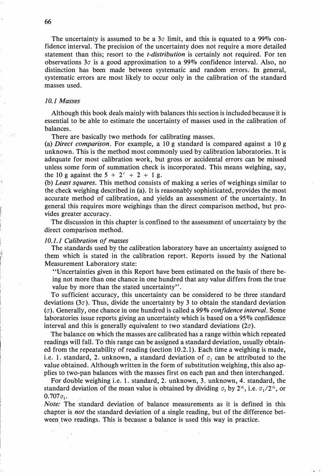
66

The uncertainty is assumed to be a 3<J limit, and this is equated to a 99% con­fidence interval. The precision of the uncertainty does not require a more detailed statement than this; resort to the t-distribution is certainly not required. For ten observations 3<J is a good approximation to a 99% confidence interval. Also, no distinction has been made between systematic and random errors. In general, systematic errors are most likely to occur only in the calibration of the standard . masses used.

JO.I Masses

Although this book deals mainly with balances this section is included because it is essential to be able to estimate the uncertainty of masses used in the calibration of balances.

There are basically two methods for calibrating masses. (a) Direct comparison. For example, a 10 g standard is compared against a 10 gunknown. This is the method most commonly used by calibration laboratories. It isadequate for most calibration work, but gross or accidental errors can be missedunless some form of summation check is incorporated. This means weighing, say,the 10 g against the 5 + 2' + 2 + 1 g.(b) Least squares. This method consists of making a series of weighings similar tothe check weighing described in (a). It is reasonably sophisticated, provides the mostaccurate method of calibration, and yields an assessment of the uncertainty. Ingeneral this requires more weighings than the direct comparison method, but pro­vides greater accuracy.

The discussion in this chapter is confined to the assessment of uncertainty by the direct comparison method.

JO.I.I Calibration of masses The standards used by the calibration laboratory have an uncertainty assigned to

them which is stated in the calibration report. Reports issued by the National Measurement Laboratory state:

"Uncertainties given in this Report have been estimated on the basis of there be­ing not more than one chance in one hundred that any value differs from the true value by more than the stated uncertainty". To sufficient accuracy, this uncertainty can be considered to be three standard

deviations (3<J ). Thus, divide the uncertainty by 3 to obtain the standard deviation (<J). Generally, one chance in one hundred is called a 99% confidence interval. Some laboratories issue reports giving an uncertainty which is based on a 95% confidence interval and this is generally equivalent to two standard deviations (2<J).

The balance on which the masses are calibrated has a range within which repeated readings will fall. To this range can be assigned a standard deviation, usually obtain­ed from the repeatability of reading (section 10.2.1). Each time a weighing is made, i.e. 1. standard, 2. unknown, a standard deviation of <J1 can be attributed to thevalue obtained. Although written in the form of substitution weighing, this also ap­plies to two-pan balances with the masses first on each pan and then interchanged.

For double weighing i.e. 1. standard, 2. unknown, 3. unknown, 4. standard, the standard deviation of the mean value is obtained by dividing <J1 by 2v,, i.e. <Ji/2v,, or 0.7070"1 , Note: The standard deviation of balance measurements as it is defined in this chapter is not the standard deviation of a single reading, but of the difference bet­ween .two readings. This is because a balance is used this way in practice.

67

To find the standard deviation of the unknown mass, it is necessary to combine the standard deviation from the balance measurements with that of the standard. This is done by squaring the standard deviations, adding them, and taking the square root. Thus, for double weighings, the standard deviation of the unknown is

[ (J2 + ( <Ji2)/2] V,

The uncertainty, at 99% confidence interval, is

I 0.1. 2 Example - calibration of a I O g mass

Consider the calibration of a 10 g mass by means of double weighing. The 10 g standard has an uncertaintyt of 10 µg and a value of 10.000 034 g. The masses are compared on a balance with a standard deviation of 20 µg. Observations: standard 10.000 00

unknown 10.000 06 unknown 10.000 07 standard 10.000 02

Difference, standard - unknown = 10.000 010 - 10.000 065 = - 0.000 055 g

Hence unknown = 10.000 034 + 0.000 055

= 10.000 089 g

Uncertainty: The standard deviation of the standard mass is 10/3 µg.

Note: If the uncertainty were based on a 95 OJo confidence interval, then the standard deviation would be 10/2 = 5 µg. However throughout this paper a 99% confidence interval (i.e., 3a) is assumed.

Uncertainty = 3[(10/3)2 + 202/2]v, = 3 X 14.53= 43.6 µg

The result could then be written as 10.000 09 ± 0.000 044 g (see aJso section 10.3).

I 0.1. 3 Calibrations requiring more than one standard

If more than one standard is used on the balance pan at the same time, then the uncertainty of the standards is given by three times the square root of the sum of the standard deviations squared

uncertainty = 3(ai2 + az2 + ... )v, ,

where o-; is the standard deviation of mass i (section 10.1.1).

t Assigned by NML (see section 10.1.1)

(24)

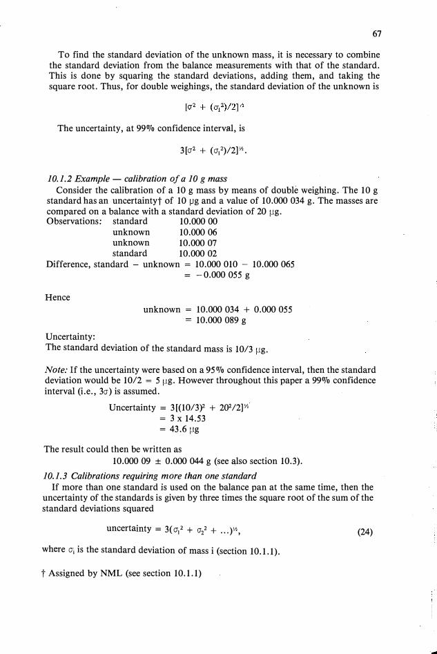
ii ( · I:: :•

66

The uncertainty is assumed to be a 3cr limit, and this is equated to a 99% con­fidence interval. The precision of the uncertainty does not require a more detailed statement than this; resort to the t-distribution is certainly not required. For ten observations 3cr is a good approximation to a 99% confidence interval. Also, no distinction has been made between systematic and random errors. In general, systematic errors are most likely to occur only in the calibration of the standard .masses used.

JO.I Masses

Although this book deals mainly with balances this section is included because it is essential to be able to estimate the uncertainty of masses used in the calibration of balances.

There are basically two methods for calibrating masses. (a) Direct comparison. For example, a 10 g standard is compared against a 10 gunknown. This is the method most commonly used by calibration laboratories. It isadequate for most calibration work, but gross or accidental errors can be missedunless some form of summation check is incorporated. This means weighing, say,the 10 g against the 5 + 2' + 2 + 1 g.(b) Least squares. This method consists of making a series of weighings similar tothe check weighing described in (a). It is reasonably sophisticated, provides the mostaccurate method of calibration, and yields an assessment of the uncertainty. Ingeneral this requires more weighings than the direct comparison method, but pro­vides greater accuracy.

The discussion in this chapter is confined to the assessment of uncertainty by the direct comparison method.

JO.I.I Calibration of masses The standards used by the calibration laboratory have an uncertainty assigned to

them which is stated in the calibration report. Reports issued by the National Measurement Laboratory state:

"Uncertainties given in this Report have been estimated on the basis of there be­ing not more than.one chance in one hundred that any value differs from the true value by more than the stated uncertainty". To sufficient accuracy, this uncertainty can be considered to be three standard

deviations (3cr ). Thus, divide the uncertainty by 3 to obtain the standard deviation (cr). Generally, one chance in one hundred is called a 99% confidence interval. Some laboratories issue reports giving an uncertainty which is based on a 95% confidence interval and this is generally equivalent to two standard deviations (2cr).

The balance on which the masses are calibrated has a range within which repeated readings will fall. To this range can be assigned a standard deviation, usually obtain­ed from the repeatability of reading (section 10.2.1). Each time a weighing is made, i.e. 1. standard, 2. unknown, a standard deviation of cr1 can be attributed to thevalue obtained. Although written in the form of substitution weighing, this also ap­plies to two-pan balances with the masses first on each pan and then interchanged.

For double weighing i.e. 1. standard, 2. unknown, 3. unknown, 4. standard, the standard deviation of the mean value is obtained by dividing cr1 by 2';,, i.e. cr/2v, , or 0.7070"1. Note: The standard deviation of balance measurements as it is defined in this chapter is not the standard deviation of a single reading, but of the difference bet­ween _two readings. This is because a balance is used this way in practice.

67

To find the standard deviation of the unknown mass, it is necessary to combine the standard deviation from the balance measurements with that of the standard. This is done by squaring the standard deviations, adding them, and taking the square root. Thus, for double weighings, the standard deviation of the unknown is

The uncertainty, at 99% confidence interval, is

3 [cr2 + ( cr?)/2] v,.

10.1.2 Example - calibration of a 10 g mass

Consider the calibration of a 10 g mass by means of double weighing. The 10 g standard has an uncertaintyt of 10 µg and a value of 10.000 034 g. The masses are compared on a balance with a standard deviation of 20 µg. Observations: standard 10.000 00

unknown 10.000 06 unknown 10.000 07 standard 10.000 02

Difference, standard - unknown = 10.000 010 - 10.000 065 = -0.000 055 g

Hence unknown = 10.000 034 + 0.000 055

10.000 089 g

Uncertainty: The standard deviation of the standard mass is 10/3 µg.

Note: If the uncertainty were based on a 95% confidence interval, then the standard deviation would be 10/2 = 5 µg. However throughout this paper a 99% confidence interval (i.e., 3cr) is assumed.

Uncertainty = 3[(10/3)2 + 202/2]v, = 3 X 14.53 = 43.6 µg

The result could then be written as 10.000 09 ± 0.000 044 g (see also section 10.3).

10.1.3 Calibrations requiring more than one standard

If more than one standard is used on the balance pan at the same time, then the uncertainty of the standards is given by three times the square root of the sum of the standard deviations squared

uncertainty= 3(cri2 + ai2 + ... )Y', (24)

where O"j is the standard deviation of mass i (section 10.1.1 ).

t Assigned by NML (see section 10.1.1)

ir: · I,.1 Ii

68

Examples

(a) Consider the calibration of an object of mass 113.32 g. The standards reqmred,

with their uncertainties, are as follows:

100 10 2 1 0.2 0.1 0.02

0.000 1 0.000 01 0.000 01 0.000 01 0.000 01 0.000 01 0.000 01

Thus, the standard deviation of all the masses is

[(100/3)2 + (10/3)2 + (10/3)2 + (10/3)2 + (10/3)2 + (10/3)2 + (10/3)2) V,

= v,(1002 + 102 + 102 + 102 + 102 + 102 + 102r,

= 35 pg whence the uncertainty = 0.000 105 g

= 0.000 11 g (see the rounding comment in section 10.3). (b) Consider the calibration of an object weighing 8.945 g. The standards used are5, 2, 1, 0.5, 0.2, 0.2, 0.02, 0.02, 0.005 g, and each has an uncertainty of 10 µg. Thestandard deviation of the sum of the 9 masses is

[(10/3)2 + (9 terms) ..... + (10/3)2) v, =' v,(9 X 102)v, = 10.Q pg.

Thus the uncertainty is 30 µg.

10.2 Balances

Most testing of balances involves placing an appropriate mass on the pan and reading the balance. This means that the uncertainty is a combination of the stan­dard deviations of the repeatability and the masses.

This can be expressed as

where

(25)

O" = standard deviation of the calibrating masses, i.e. uncertainty on the Laboratory's Report divided by 3, standard deviation of the repeatability of reading (sections 4.1, 5;1, 6.3),

k = number of readings used to make the measurements (k = 2 for double weighing),

U = uncertainty of the test under consideration (assumed to be 3 times the standard deviation).

This is the basic equation used in the estimation of uncertainty, and its use in estimating the uncertainty of the different tests is illustrated by examples in the following sections.

For the sake of clarity in the following examples, any mass standard used for the calibrations is assumed to have a correction of zero. The size of the correction is not

related in any way to the uncertainty. It is also assumed that the masses have been

69

calibrated by the National Measurement Laboratory and thus have an uncertainty (3o-) of 1 part in 106 or 10 µg, whichever is the greater.

10.2.1 Repeatability of reading

The formulae for calculating the repeatability of reading are given in sections 4.1, 5.1 and 6.3. The uncertainty is given by

10.2.2 Sensitivity and scale value The uncertainty in the sensitivity is obtained from the uncertainty in the

calibrating mass (10.1.1) and the repeatability of reading (10.2.1), and is given by equation (25). This does not apply to the sensitivity reciprocal for two-pan balances (see 4.11.2).

Sometimes, as in comparing nearly equal masses, only the first, say, 50Jo of the scale is used. In these cases the uncertainty in the sensitivity can be reduced in pro­portion. For example, if the sensitivity is measured over a range (scale) of 100 units but the balance is used only over the first five units, then the uncertainty due to the calibrating mass is reduced by a factor of 20 and

U = 3[(a/20)2 + a//k]v,.

This applies particularly to balances with sensitivities of less than 10 µg per divi­sion, which is smaller than the uncertainty of the calibrating mass. 10.2.3 Uniformity of scale and departure from nominal value

For each point tested, this is again a combination of the uncertainty in the calibrating mass (10.1.1) and the repeatability of reading (10.2.1). Example

Consider a balance with a scale of range 1 g and 100 divisions (1 div = 10 mg) which can be read to 0.1 division (1 mg). The uniformity of scale is tested at half and full scale. This is done by placing a 0.5 g and then a 1.0 g standard on the pan. Observations:

Corrections:

half scale

0.000 0.498 0.494

-0.002

Half scale + 0.003 g

full scale 0.000 I.OOO0.999

-0.001

Full scale 0.000 g

If the balance has o-1 = 0.002 g, then (from equation (25)) the uncertainty at both half and full scale is

U = 3[(0.01/3)2 + (2/2v,)2]v, mg 3(0.000 012 + 2)v,

= 4.3 mg.

Thus, at half scale, the balance has a correction due to errors in the scale of + 3 mg, and this has been determined with an uncertainty of 4.3 mg. Note: Whenthe uncertainty is larger than the correction, that correction is not significantly dif­ferent from zero. Thus, in the above example, the most probable value is 3 mg, andthis should be used. However the balance user is quite entitled to use a correction ofzero.

68

Examples (a) Consider the calibration of an object of mass 113.32 g. The standards required,with their uncertainties, are as follows:

100 10 2 1 0.2 0.1 0.02

0.000 1 0.000 01 0.000 01 0.000 01 0.000 01 0.000 01 0.000 01

Thus, the standard deviation of all the masses is

[(100/3)2 + (10/3)2 + (10/3)2 + (10/3)2 + (10/3)2 + (10/3)2 + (10/3)2] \/i

= V, 0 002 + 102 + 102 + 102 + 102 + 102 + 102v,,

= 35 µg whence the uncertainty = 0.000 105 g

= 0.000 11 g (see the rounding comment in section 10.3). (b) Consider the calibration of an object weighing 8.945 g. The standards used are5, 2, 1, 0.5, 0.2, 0.2, 0.02, 0.02, 0.005 g, and each has an uncertainty of 10 µg. Thestandard deviation of the sum of the 9 masses is

[(10/3)2 + (9 terms) ..... + (10/3)2] v, =' v,(9 X 102)\/i = 10.0 µg.

Thus the uncertainty is 30 µg.

10.2 Balances

Most testing of balances involves placing an appropriate mass on the pan and reading the balance. This means that the uncertainty is a combination of the stan­dard deviations of the repeatability and the masses.

This can be expressed as

where

u (25)

a - standard deviation of the calibrating masses, i.e. uncertainty on the Laboratory's Report divided by 3,

a1 standard deviation of the repeatability of reading (sections 4.1, 5.1, 6.3),

k = number of readings used to make the measurements (k = 2 for double weighing),

U = uncertainty of the test under consideration (assumed to be 3 times the standard deviation).

This is the basic equation used in the estimation of uncertainty, and its use in estimating the uncertainty of the different tests is illustrated by examples in the following sections.

For the sake of clarity in the following examples, any mass standard used for the calibrations is assumed to have a correction of zero. The size of the correction is not

related in any way to the uncertainty. It is also assumed that the masses have been

r l

69

calibrated by the National Measurement Laboratory and thus have an uncertainty (3u) of 1 part in 106 or 10 µg, whichever is the greater.

10.2.1 Repeatability of reading The formulae for calculating the repeatability of reading are given in sections 4.1,

5.1 and 6.3. The uncertainty is given by

10.2.2 Sensitivity and scale value The uncertainty in the sensitivity is obtained from the uncertainty in the

calibrating mass (10.1.1) and the repeatability of reading (10.2.1), and is given by equation (25). This does not apply to the sensitivity reciprocal for two-pan balances (see 4.11.2).

Sometimes, as in comparing nearly equal masses, only the first, say, 50Jo of the scale is used. In these cases the uncertainty in the sensitivity can be reduced in pro­portion. For example, if the sensitivity is measured over a range (scale) of 100 units but the balance is used only over the first five units, then the uncertainty due to the calibrating mass is reduced by a factor of 20 and

U = 3[(u/20)2 + a?lk]Yi.

This applies particularly to balances with sensitivities of less than 10 µg per divi­sion, which is smaller than the uncertainty of the calibrating mass. 10.2.3 Uniformity of scale and departure from nominal value

For each point tested, this is again a combination of the uncertainty in the calibrating mass (10.1.1) and the repeatability of reading (10.2.1). Example

Consider a balance with a scale of range 1 g and 100 divisions (1 div = 10 mg) which can be read to 0.1 division (1 mg). The uniformity of scale is tested at half and full scale. This is done by placing a 0.5 g and then a 1.0 g standard on the pan. Observations:

Corrections:

half scale 0.000 0.498 0.494

-0.002

Half scale + 0.003 g

full scale 0.000 1.000 0.999

-0.001

Full scale 0.000 g

If the balance has a1 = 0.002 g, then (from equation (25)) the uncertainty at both half and full scale is

U 3 [(0.01/3)2 + (2/2Yi)2] Yi mg = 3(0.000 012 + 2)Yi = 4.3 mg.

Thus, at half scale, the balance has a correction due to errors in the scale of + 3 mg, and this has been determined with an uncertainty of 4.3 mg. Note: Whenthe uncertainty is larger than the correction, that correction is not significantly dif­ferent from zero. Thus, in the above example, the most probable value is 3 mg, andthis should be used. However the balance user is quite entitled to use a correction ofzero.

I '

ii

I :j ! II i

i ! ! i

I I ' d i !I,!

I

70

10.2.4 Effect of off-centre loading

This is the change in reading observed when a mass is placed on different parts of the pan. The uncertainty of the reading at each position of the mass is the uncertain­ty due to the repeatability of the balance, U1

•

10.2.5 Masses installed in the balance

The uncertainty of the dial settings for each of the methods described in section , 5.8 (except least squares) can be estimated by appropriate use of equation (25).

In general, there are very few balance users who actually apply corrections for dial readings. Most want to know whether the corrections to the dial readings conform to the tolerances laid down by the manufacturer, or if the balance is sufficiently ac­curate for their purpose.

To decide whether the correction determined for a particular dial ·setting is within the manufacturer's specification, the uncertainty must be calculated. This is done by combining the standard deviation with the uncertainty due to the standards.

If T is the manufacturer's tolerance, C is the magnitude of the correction, and C� T + U,

then the dial setting will give a mass reading that conforms to the manufacturer's specification. To express it another way, the dial reading conforms if the correction is less than or equal to the sum of the manufacturer's tolerance and the uncertainty.

Manufacturers' statements regarding accuracy, or tolerances, of built-in masses are sometimes ambiguous. Hence in some cases there could be doubt as to whether the masses conform. If possible T should be recalculated to be a 30' limit. However 30' is considered to be quite severe for tolerance testing and so, in general, only the values should be reported without drawing any conclusions. Example

A 100 g balance has a readability of 0.1 mg and a repeatability of reading of 0.15 mg. The manufacturer's tolerance on the built-in masses is 0.2 mg. The calibra­tion is made at a dial setting of 90 g. Observations:

zero 90 90

zero Correction = -0.45 mg Standard deviation of standards:

50 g 0.05/3 mg 20 g 0.02/3 mg 20 g 0.02/3 mg.

mg

0.0 0.4 0.5 0.0.

Standard deviation of repeatability of reading is 0.15/2Vz mg (cf. section 10.1.1). Then

u = 3[(0.05/3)2 + (0.02/3)2 + (0.02/3)2 + (0.15/2Vz)2]Vz = 0.33 mg,

and T + U = 0.2 + 0.33 = 0.53 mg,

which is larger than the magnitude of the correction 0.45 mg. Hence, the masses us­ed in dial setting 90 could be said to conform to the manufacturer's specification, but a more accurate analysis (least squares - chapter 9) may be required.

71

10.2.6 Other tests

It is not usual to quote an uncertainty for the remaining tests. Often the measure­ment is done merely to indicate the magnitude so that the balance can be adjusted, e.g. ratio of arms, parallelism of knife edges, etc. In all cases the uncertainty can becalculated if desired. For the ratio of arms (section 4.4) this is given by

standard deviation = 1.220'/M.106 parts per million.

10.3 Number of Decimal Places Quoted

The uncertainty should be quoted to no more than two significant figures and it should always be rounded up. The quantity to which the uncertainty belongs should be quoted to the same number of decimal places, where here rounding may be up or down. In the example in section 10.1.2 it would probably be best to express the result as

10.000 09 ± 0.000 05 g.

10.4 Limit of Performance for a Balance

A balance is a reasonably complex piece of equipment and a report describes a number of different aspects, not always readily understood by the user. The ques­tion is how to decide from the balance calibration report, or even from the manufac­turer's specification, whether the balance is sufficiently accurate for the application. The aim of this section is to show how a figure called limit of performance may be calculated and used to describe how accurately a balance may weigh.

There are two different cases which depend upon how the balance is to be used: (a) no corrections are applied - limit of performance, F.(b) appropriate corrections are applied - uncertainty of weighing, H.

In general these two cases will give figures that differ by a factor of two or more.The limit of performance should be reported, as this is what most users require, and the uncertainty of weighing should be reported only if requested.

The numbers are calculated using the following assumptions: (a) weighings are made symmetrically (section 5.7.2), i.e. any drift in the readings iseliminated;(b) all miscellaneous effects [i.e. those not explicitly listed in equations (26) and (27)]are zero;(c) the effect of air buoyancy is ignored; and(d) because most balance users place objects to be weighed in the centre of the pan,the effect of off-centre loading is assumed to be zero.

The formulae given below refer only to two-knife-edge and electromagnetic-force­compensation (electronic) balances. For two-pan balances the repeatability of reading (section 4.1) is the best figure to use for the uncertainty of weighing. The assessment of this will depend upon how the balance is to be used. 10. 4.1 Balance for which no corrections are applied - limit of performance

F = 3<Ymax + magnitude of the maximum correction calculated from the unifor­mity of scale (section 5.3) or the departure from nominal value (section 6.2) + magnitude of the maximum correction of any built-in masses (section 5.8),

(26)

where crmax is the maximum value of the standard deviation of the repeatability of reading, obtained from either equation (8) or (14).

·i

70

10.2.4 Effect of off-centre loading

This is the change in reading observed when a mass is placed on different parts of the pan. The uncertainty of the reading at each position of the mass is the uncertain­ty due to the repeatability of the balance, U1 •

10.2.5 Masses installed in the balance

The uncertainty of the dial settings for each of the methods described in section . 5.8 (except least squares) can be estimated by appropriate use of equation (25).

In general, there are very few balance users who actually apply corrections for dial readings. Most want to know whether the corrections to the dial readings conform to the tolerances laid down by the manufacturer, or if the balance is sufficiently ac­curate for their purpose.

To decide whether the correction determined for a particular dial setting is within the manufacturer's specification, the uncertainty must be calculated. This is done by combining the standard deviation with the uncertainty due to the standards.

If T is the manufacturer's tolerance, C is the magnitude of the correction, and C� T + U,

then the dial setting will give a mass reading that conforms to the manufacturer's specification. To express it another way, the dial reading conforms if the correction is less than or equal to the sum of the manufacturer's tolerance and the uncertainty.

Manufacturers' statements regarding accuracy, or tolerances, of built-in masses are sometimes ambiguous. Hence in some cases there could be doubt as to whether the masses conform. If possible T should be recalculated to be a 3a limit. However 3a is considered to be quite severe for tolerance testing and so, in general, only the values should be reported without drawing any conclusions. Example

A 100 g balance has a readability of 0.1 mg and a repeatability of reading of 0.15 mg. The manufacturer's tolerance on the built-in masses is 0.2 mg. The calibra­tion is made at a dial setting of 90 g. 0 bservati ons:

zero 90 90

zero Correction = - 0.45 mg Standard deviation of standards:

50 g 0.05/3 mg 20 g 0.02/3 mg 20 g 0.02/3 mg.

mg 0.0 0.4 0.5 0.0.

Standard deviation of repeatability of reading is 0.15/2v, mg (cf. section 10.1.1). Then

u = 3[(0.05/3)2 + (0.02/3)2

+ (0.02/3)2 + (0.15!2V2)2]V,= 0.33 mg,

and T + U = 0.2 + 0.33 = 0.53 mg,

which is larger than the magnitude of the correction 0.45 mg. Hence, the masses us­ed in dial setting 90 could be said to conform to the manufacturer's specification, but a more accurate analysis (least squares - chapter 9) may be required.

71

10.2. 6 Other tests

It is not usual to quote an uncertainty for the remaining tests. Often the measure­ment is done merely to indicate the magnitude so that the balance can be adjusted, e.g. ratio of arms, parallelism of knife edges, etc. In all cases the uncertainty can becalculated if desired. For the ratio of arms (section 4.4) this is given by

standard deviation = 1.22a /M.106 parts per million .

10.3 Number of Decimal Places Quoted

The uncertainty should be quoted to no more than two significant figures and it should always be rounded up. The quantity to which the uncertainty belongs should be quoted to the same number of decimal places, where here rounding may be up or down. In the example in section 10.1.2 it would probably be best to express the result as

10.000 09 ± 0.000 05 g.

10.4 Limit of Performance for a Balance

A balance is a reasonably complex piece of equipment and a report describes a number of different aspects, not always readily understood by the user. The ques­tion is how to decide from the balance calibration report, or even from the manufac­turer's specification, whether the balance is sufficiently accurate for the application. The aim of this section is to show how a figure called limit of performance may be calculated and used to describe how accurately a balance may weigh.

There are two different cases which depend upon how the balance is to be used: (a) no corrections are applied - limit of performance, F.(b) appropriate corrections are applied - uncertainty of weighing, H.

In general these two cases will give figures that differ by a factor of two or more.The limit of performance should be reported, as this is what most users require, and the uncertainty of weighing should be reported only if requested.

The numbers are calculated using the following assumptions: (a) weighings are made symmetrically (section 5.7.2), i.e. any drift in the readings iseliminated;(b) all miscellaneous effects [i.e. those not explicitly listed in equations (26) and (27)]are zero; (c) the effect of air buoyancy is ignored; and(d) because most balance users place objects to be weighed in the centre of the pan,the effect of off-centre loading is assumed to be zero.

The formulae given below refer only to two-knife-edge and electromagnetic-force­compensation (electronic) balances. For two-pan balances the repeatability of reading (section 4.1) is the best figure to use for the uncertainty of weighing. The assessment of this will depend upon how the balance is to be used.

10.4.1 Balance for which no corrections are applied - limit of performance F = 3<Ymax + magnitude of the maximum correction calculated from the unifor­mity of scale (section 5.3) or the departure from nominal value (section 6.2) + magnitude of the maximum correction of any built-in masses (section 5.8),

(26)

where o-max is the maximum value of the standard deviation of the repeatability of reading, obtained from either equation (8) or (14).

'

'

I

72

Note: The correction for any built-in masses should be the sum of corrections for all the masses. However, as this is rarely determined, the maximum value is the best figure available. The built-in masses are usually specified as "accuracy: each weight combination < ± X g" in the manufacturer's specification, and this is the figure that should be used.

10.4.2 Balance for which corrections are applied - uncertainty of weighing

where a max

is defined in section 10.4.1.,

(27)

U1

is the uncertainty due to the uniformity of scale or the departure from nominal value (section 10.2.3), U2

is the uncertainty in the calibration of the built-in masses (section 10.2.5).

Note: Because the corrections have been applied to the balance the uncertainties of these corrections have been used in equation (27), whereas the actual magnitudes of the corrections are used in equation (26).

10.4.3 Meaning of the limit of performance The numerical value calculated by means of equation (26) can be interpreted as

follows. If the balance is in an ideal environment (as defined in Appendix 1), then the

readings on the balance will give the correct mass of an object (on the 8.0 basis -chapter 8) within the limit of performance ( ± F). It is estimated that there is not more than one chance in one hundred that any value differs from the correct value by more than ± F. Thus if m is the balance reading, the mass of the object lies in the range m ± F.

It is emphasised that the limit of performance, F, is an upper bound. In many ap­plications the balance may weigh more accurately than this figure.

On the balance report this figure could be reported as follows:

Limit of performance for the balance = ± ..... g.

10.4.4 Meaning of the uncertainty of weighing The numerical value calculated by means of equation (27) can ·be interpreted as

follows. If the balance is in an ideal environment (as defined in Appendix 1), then the

readings on the balance will, after the appropriate corrections have been applied, give the correct mass of an object (on the 8.0 basis - chapter 8) within the uncer­tainty of weighing ( ± H). It is estimated that there is not more than one chance in one hundred that any value differs from the correct value by more than ± H. Thus if m is the value obtained the mass of the object lies in the range m ± H.

The uncertainty of weighing should not be reported unless all the built-in masses in the balance have been calibrated.

10. 4. 5 Numerical examples1. Two-knife-edge balance - consider the Report given in section 5 .10.8.Limit of performance (equation (26))

F 3x0.10 + 0.50 + 4.4 = 5.2 mg.

Uncertainty of weighing (equation (27))

H = [(3x0.10)2 + 0.092 + o.22p1z

= 0.37 mg. 2. Electronic balance - consider the Report given in section 6.11.7.Limit of performance (equation (26))

F = 3x0.003 + 0.05 = 0.06 g.

Uncertainty of weighing (equation (27)) H = [(3x0.003)2 + O.Ol2]';,

= 0.014 g. 3. Two-knife-edge balance - manufacturer's specification

Discrimination 0.1 mg Standard deviation ± 0.05 mg Optical scale accuracy ± 0 .1 mg Built-in masses, accuracy of each combination ± 0.18 mg

Limit of performance (equation (26)) F = 3x0.05 + 0.1 + 0.18

= 0.43 mg.

73

Uncertainty of weighing (equation (27)) H = 3[0.052 + 0.052 + o.o52p1z

= 0.26 mg. This assumes that the corrections to the scale and the masses can be measured with

a standard deviation equal to the standard deviation of the balance. This assumption

may be a little optimistic, but it is a reasonable guide for the selection of a balance.

4. Electronic balance - manufacturer's specification

Discrimination 0.01 gStandard deviation ±0.01 g

(for this calculation the standard deviation is assumed to be 0.0033 g, see sec-

tion 6.3) Linearity deviation ±0.015 g

Limit of performance (equation (26)) F = 3x0.0033 + 0.015

= 0.025 g. Uncertainty of weighing (equation (27))

H = 3[0.00332 + 0.00332]v,

= 0.014 g.

n 1, ' i :

i I 111 ; !'J I i., '"

I·,

! -,

72

Note: The correction for any built-in masses should be the sum of corrections for all the masses. However, as this is rarely determined, the maximum value is the best figure available. The built-in masses are usually specified as "accuracy: each weight combination -< ± X g" in the manufacturer's specification, and this is the figure that should be used.

10.4.2 Balance for which corrections are applied - uncertainty of weighing

where amax is defined in section 10.4.1.,

(27)

U1 is the .uncertainty due to the uniformity of scale or the departure from nominal value (section 10.2.3), U2

is the uncertainty in the calibration of the built-in masses (section 10.2.5).

Note: Because the corrections have been applied to the balance the uncertainties of these corrections have been used in equation (27), whereas the actual magnitudes of the corrections are used in equation (26).

10.4.3 Meaning of the limit of performance

The numerical value calculated by means of equation (26) can be interpreted as follows.

If the balance is in an ideal environment (as defined in Appendix 1), then the readings on the balance will give the correct mass of an object (on the 8.0 basis -

· chapter 8) within the limit of performance ( ± F). It is estimated that there is notmore than one chance in one hundred that any value differs from the correct valueby more than ±F. Thus if m is the balance reading, the mass of the object lies in therange m ± F.

It is emphasised that the limit of performance, F, is an upper bound. In many ap­plications the balance may weigh more accurately than this figure.

On the balance report this figure could be reported as follows:

Limit of performance for the balance = ± ..... g.

10.4.4 Meaning of the uncertainty of weighing The numerical value calculated by means of equation (27) can ·be interpreted as

follows. If the balance is in an ideal environment (as defined in Appendix 1), then the

readings on the balance will, after the appropriate corrections have been applied, give the correct mass of an object (on the 8.0 basis - chapter 8) within the uncer­tainty of weighing ( ± H). It is estimated that there is not more than one chance in one hundred that any value differs from the correct value by more than ± H. Thus if m is the value obtained the mass of the object lies in the range m ± H.

The uncertainty of weighing should not be reported unless all the built-in masses in the balance have been calibrated.

10.4.5 Numerical examples

1. Two-knife-edge balance - consider the Report given in section 5 .10.8.Limit of performance (equation (26))

F = 3x0.10 + 0.50 + 4.4 = 5.2 mg.

Uncertainty of weighing (equation (27)) H = [(3x0.10)2

+ 0.092 + 0.22] v,

= 0.37 mg. 2. Electronic balance - consider the Report given in section 6.11. 7.Limit of performance (equation (26))

F = 3x0.003 + 0.05

= 0.06 g. Uncertainty of weighing (equation (27))

H = [(3x0.003)2 + O.Ol2]Y' = 0.014 g.

3. Two-knife-edge balance - manufacturer's specification

Discrimination 0.1 mgStandard deviation ± 0.05 mgOptical scale accuracy ± 0 .1 mgBuilt-in masses, accuracy of each combination ± 0.18 mg

Limit of performance (equation (26)) F = 3x0.05 + 0.1 + 0.18

= 0.43 mg.

73

Uncertainty of weighing (equation (27)) H = 3[0.052 + 0.052 + 0.052] v,

= 0.26 mg.

This assumes that the corrections to the scale and the masses can be measured with

a standard deviation equal to the standard deviation of the balance. This assumption

may be a little optimistic, but it is a reasonable guide for the selection of a balance.

4. Electronic balance - manufacturer's specification

Discrimination 0.01 gStandard deviation ± 0.01 g

(for this calculation the standard deviation is assumed to be 0.0033 g, see sec-

tion 6.3) Linearity deviation ± 0.015 g

Limit of performance (equation (26)) F = 3x0.0033 + 0.015

= 0.025 g. Uncertainty of weighing (equation (27))

H 3[0.00332 + 0.00332] Y'

= 0.014 g.

74

11. References

ASTM (1968). "Standard Methods of Testing Single-Arm Balances" E319.

Australian Standard (1980). "Glossary of Terms used in Metrology Part 1 - General Terms and

Definitions" 1514.

Bell, G.A. (1955). "The Calibration of the Weights in Balances with Automatic Weight Loading". NSL Technical Paper No. 6.

Bietry, L., Kochsiek, M. (1983). "Mettler Dictionary of Weighing Terms" (Mettler Instruments AG).

Bignell, N. (1983). Estimation of the centre of swing of an under-damped balance. Metrologia 19, 127.

Giacomo, P. (1982). Equation for the determination of the density of moist air. Metrologia 18, 33-40.

Glazebrook, R. (ed.) (1950). "A Dictionary of Applied Science" Vo! 3, 107-126 (Peter Smith: New York).

Humphries, J.W. (1960). The calibration of weights built into a balance. Aust J. App. Sci. 11, 360.Lashof, T.W., Macurdy, L.B. (1954). Testing a quick-weighing balance. Analytical Chemistry 26, 707.NPL Notes on Applied Science (1954). "Balances, weights and precise laboratory weighing" No. 7

(HMSO).

OIML (1978). "Vocabulary of Legal Metrology" (Organization Internationale de Metrologie Legale).

Pontius, P.E. (1974). "Mass and Mass Values" NBS Monograph 133.

Prowse, D.B. (1984). Calibration of masses Jn "Modern Techniques in Metrology" (Ed. P. Hewitt), pp

33-54 (World Scientific: Singapore).

Telarc (1982). "A User's Guide to the Calibration of Laboratory Balances" Technical Note No. I.

Illustrations have been reproduced from:

'Mettler Dictionary of Weighing Terms', Mettler Instrumente AG, 1983.

'Measuring Instruments: tools of knowledge and control', Peter Peregrinus Ltd, in association with

the Science Museum, London, 1979. 'Dictionary of Applied Physics', vol. 3, Peter Smith, New York, 1950.

75

APPENDIX 1. The Balance and its Environment

A balance performs best in an "ideal" environment. This can be defined as one where further improvements make no change to the performance of the balance. It is of course almost impossible to quantify and the requirements change with the sen­sitivity and type of balance. In general the more sensitive the balance the better the environment that is required.

This appendix gives a general guide to the principles involved in deciding whether the location of a balance is satisfactory. The general constraints of economy and space will sometimes be the overriding consideration.

.A.I.I 'J'emperature

The room temperature should be stable. The actual value of the temperature is relatively unimportant; it is the stability that matters. Small fluctuations around a mean have little effect on most balances. But continual increase or decrease in temperatures during the day results in a continual change in reading. For all types of balances, temperature changes cause gradients in the balance mechanism, resulting in drift in the reading and sometimes change in the sensitivity.

If possible the temperature of the balance room should not change by �ore tha_n+ 2 or 3 °C during any eight-hour period. If the room cools down at mght but isstable during the day, then the balance will spend most of the day reaching equilibrium with the room, and hence the reading will drift even though the room temperature is stable. The 2 or 3 °C stability is what is ideally req�ir�d for bala�ce calibration, but less stringent conditions can be tolerated for weighmg dependmg upon the accuracy required.

.A.I.2 Humidity

This is relatively unimportant, but conditions should never be allowed to reach the point where condensation is likely to occur. For high precision weighing relativelr stable humidity i.e. constant to ±50Jo, is desirable to minimise surface effects .

.A.I.3 .A.ir Currents

Along with temperature changes, air currents probably cause the greatest distur­bance to balance readings. For analytical balances significant air currents are caused by temperature gradients. These often result from the operator sittin� in front of.thebalance or from placing a hand inside the balance case. When this happens time must be allowed for the balance and the environment to stabilise. Research has shown that if a stable temperature gradient is induced, with the temperature significantly higher (1 or 2°C) at the top of the balance case than at the bottom, then air currents are greatly reduced. This however is not a practical solution for most users of precision balances.

An air current of velocity 4.6 cm/s impinging normally on a pan of area 78 c°:2

(10 cm diameter) produces a force equivalent to a mass of 1 mg on the pan. The a�r speed in an air-conditioned laboratory is typically �bout 30 cm/s. 1:'he effec! 1s directly proportional to the squares of both the pan diameter and the air speed, 1.e. doubling either of these parameters produces four time� the force on the bala�ce pan. Thus, draught shields can be seen to be essential for reasonably precise weighing with top-loading balances.

Ii

I

74

11. References

ASTM (1968). "Standard Methods of Testing Single-Arm Balances" E319.

Australian Standard (1980). "Glossary of Terms used in Metrology Part l - General Terms and Definitions" 1514.

Bell, G.A. (1955). "The Calibration of the Weights in Balances with Automatic Weight Loading". NSLTechnical Paper No. 6.

Bietry, L., Kochsiek, M. (1983). "Mettler Dictionary of Weighing Terms" (Mettler Instruments AG).Bignell, N. (1983). Estimation of the centre of swing of an under-damped balance. Metrologia 19, 127.Giacomo, P. (1982). Equation for the determination of the density of moist air. Metrologia 18, 33-40.Glazebrook, R. (ed.) (1950). "A Dictionary of Applied Science" Vol 3, 107-126 (Peter Smith: New

York).

Humphries, J.W. (1960). The calibration of weights built into a balance. Aust J. App. Sci. 11, 360.Lashof, T.W., Macurdy, L.B. (1954). Testing a quick-weighing balance. Analytical Chemistry 26, 707.NPL Notes on Applied Sdence (1954). "Balances, weights and precise laboratory weighing" No. 7

(HMSO).

OIML (1978). "Vocabulary of Legal Metrology" (Organization Internationale de Metrologie Legale).

Pontius, P.E. (1974). "Mass and Mass Values" NBS Monograph 133.

Prowse, D.B. (1984). Calibration of masses Jn "Modern Techniques in Metrology" (Ed. P. Hewitt), pp 33-54 (World Scientific: Singapore).

Telarc (1982). "A User's Guide to the Calibration of Laboratory Balances" Technical Note No. 1.

Illustrations have been reproduced from:

'Mettler Dictionary of Weighing Terms', Mettler Instrumente AG, 1983. 'Measuring Instruments: tools of knowledge and control', Peter Peregrinus Ltd, in association with

the Science Museum, London, 1979. 'Dictionary of Applied Physics', vol. 3, Peter Smith, New York, 1950.

75

APPENDIX 1. The Balance and its Environment

A balance performs best in an "ideal" environment. This can be defined as one where further improvements make no change to the performance of the balance. It is of course almost impossible to quantify and the requirements change with the sen­sitivity and type of balance. In general the more sensitive the balance the better the environment that is required.

This appendix gives a general guide to the principles involved in deciding whether the location of a balance is satisfactory. The general constraints of economy and space will sometimes be the overriding consideration.

.A.I.I 1'ern])erature

The room temperature should be stable. The actual value of the temperature is relatively unimportant; it is the stability that matters. Small fluctuations around a mean have little effect on most balances. But continual increase or decrease in temperatures during the day results in a continual change in reading. For all types of balances, temperature changes cause gradients in the balance mechanism, resulting in drift in the reading and sometimes change in the sensitivity.

If possible the temperature of the balance room should not change by �ore tha.n+2 or 3 °c during any eight-hour period. If the room cools down at mght but isstable during the day, then the balance will spend most of the day reaching equilibrium with the room, and hence the reading will drift even though the room temperature is stable. The 2 or 3 °C stability is what is ideally req�in:d for bala�ce calibration, but less stringent conditions can be tolerated for weighmg dependmg upon the accuracy required.

.A.1.2 Humidity

This is relatively unimportant, but conditions should never be allowed to reach the point where condensation is likely to occur. For high precision weighing relativelr stable humidity i. e. constant to ±50Jo, is desirable to minimise surface effects .

.A.1.3 .A.ir Currents

Along with temperature changes, air currents probably cause the greatest distur­bance to balance readings. For analytical balances significant air currents are caused by temperature gradients. These often result from the operator sittin� in front of_thebalance or from placing a hand inside the balance case. When this happens time must be allowed for the balance and the environment to stabilise. Research has shown that if a stable temperature gradient is induced, with the temperature significantly higher (1 or 2°C) at the top of the balance case than at the bottom, then air currents are greatly reduced. This however is not a practical solution for most users of precision balances.

An air current of velocity 4.6 cm/s impinging normally on a pan of area 78 cn:2

(10 cm diameter) produces a force equivalent to a mass of 1 mg on the pan. The a�r speed in an air-conditioned laboratory is typically about 30 cm/s. 1:he effec! 1s directly proportional to the squares of both the pan diameter and the a1r speed, 1.e. doubling either of these parameters produces four time� the force on the bala�ce pan. Thus, draught shields can be seen to be essential for reasonably precise weighing with top-loading balances.

76

Al.4 Vibration

All balances are susceptible to vibration to a greater or a lesser degree. Severe vibration will damage the knives of knife-edge balances and blur the image of op­tical readout systems. Electronic filtering and the appropriate choice of time con­stants (often via a microprocessor) can help minimise the effects of vibration on the display of force-compensation balances. Most manufacturers incorporate these op-

. tions into the electronics associated with the balance. Beam balances measure tilt and hence are very sensitive to change in level of the

balance. Therefore the use of anti-vibration mounts to eliminate vibration is not always a satisfactory solution (Al.6 (c)). This is particularly so for balances with a weighing capacity of 1 kg or more, because moving masses around on the bench may change the balance reading. This applies even to electromagnetic-force­compensation balances which are not quite so sensitive to change in level. The only real solution is a solid bench in a vibration-free environment.

Al.5 Atmospheric Pressure

The pressure in a balance room will always follow ambient pressure unless extra­ordinary precautions are taken to seal (and strengthen) the room. However these are not necessary, as the only effect of pressure changes is to alter the buoyancy and this can be measured and allowed for (chapter 8) if necessary.

An air-conditioned room will often be at a slightly higher pressure than ambient (approximately 40 Pa (0.3 mmHg)) and opening the door will cause a pressure pulse which may disturb the balance. This pressure pulse can also occur in a reasonably well-sealed room when the door is opened. In these situations the door should be locked during weighing.

Al.6 Balance Bench

The following is a list of the desirable qualities for the construction and siting of a balance bench.

(a) The bench should be made of stone, e;g, marble, granite, slate, terrazzo, etc.,and be a minimum of about 40 mm thick. It should not be made of reinforced con­crete because of possible magnetic effects of the reinforcing.

(b) The bench should preferably be mounted on brick pillars on a concrete floorand free from any wall. The bench should not be made of timber or mounted on a wooden floor. The floor should be the ground or basement floor of the building. It should not be a suspended floor.

(c) The bench should be placed directly on top of the pillars without anti-vibrationmountings (see section Al.4). At most, sheet lead or thin cork could be used.

(d) The pillars should be spaced so that one balance is placed mid-way betweentwo pillars. It is better if the bench tops for each balance are separate slabs of material.

(e) The bench should be sited in a room free from vibration due to machinery,passing traffic, etc. A lot of vibration is transmitted through the floor, and if this is the case an independent foundation should be made for the bench. This will mean going to a depth of about one metre, preferably on to rock. Care should then be taken to ensure that this foundation is completely free from the floor.

(f) For temperature stability an internal room with artificial lighting is better thana room with air-conditioning. Failing an internal room, choose a room on the south side. If neither of these options is available then the windows should have outside

77

sun shields. In general it is better not to air-condition if adequate temperature

stability can be obtained without it.

(g) The flow of air from any air-conditioning must be directed away from the

balance bench. (h) Any surfaces such as concrete, which are likely to give off dust should be seal-

ed.

Al. 7 Conclusion

The principles outlined in this appendix are for the ideal case. It may be necessary for the balance user to compromise with some of the conditions depending upon the type of balance and the accuracy required. As a guide it can be stated that to obtain weighing accuracies of better than 1 part in 106 there is almost no roqm for com­promise.

APPENDIX 2. Care and Handling of Masses

A2. l Types of Masses

The calibration of balances requires masses that are adequate in accuracy and

denomination for the balance being examined. Therefore once a set of masses has

been obtained and calibrated it is important that they be handled properly. The aim

of this appendix is to give some guidance as to how this may be done.

Masses can be classified into four categories depending upori their material and

type of construction: (a) integral masses made from a non-magnetic stainless steel;

(b) non-integral or two-piece masses made from non-magnetic stainless steel. The

mass value can be adjusted by the addition or removal of material from a small com­

partment - usually underneath the screw knob;

(c) masses made from brass (plated or unplated, integral or non-integral);

(d) cast-iron masses, usually painted.For the calibration of normal industrial and commercial weighing equipment

masses of types (c) and (d) are adequate and these may be picked up with bare hands. For the calibration of laboratory balances masses of types (a) or (b) are con­sidered essential, although plated masses of type (c) in good condition may be ade­quate. These of course should never be picked up with bare hands.

The National Measurement Laboratory will calibrate masses of types (a) and (b) with an uncertainty of 1 part in 106, or 10 µg, whichever is the greater. For special purposes, masses can be calibrated with a smaller uncertainty. Although the Laboratory does not prescribe recalibration periods, it recommends that masses of type (a) be recalibrated every five years and type (b) every three years.

A2.2 Handling of Masses

Masses, except types (c) and (d), should never be touched with bare hands. The small masses should be handled with bone- or plastic-tipped tweezers and the large masses with clean gloves (chamois, cotton or plastic), or the lifting tool provided. Stainless-steel tweezers, handled carefully, can be used to pick up the fractional (milligram) masses.

'Iii!

I II .II:·!

·1 ;J i iiI;;ti

I; I .I

,I , I I .j

! ·i! !

Ii

ii

1 :I

76

Al.4 Vibration

All balances are susceptible to vibration to a greater or a lesser degree. Severe vibration will damage the knives of knife-edge balances and blur the image of op­tical readout systems. Electronic filtering and the appropriate choice of time con­stants (often via a microprocessor) can help minimise the effects of vibration on the display of force-compensation balances. Most manufacturers incorporate these op-

. tions into the electronics associated with the balance. Beam balances measure tilt and hence are very sensitive to change in level of the

balance. Therefore the use of anti-vibration mounts to eliminate vibration is not always a satisfactory solution (Al .6 (c)). This is particularly so for balances with a weighing capacity of 1 kg or more, because moving masses around on the bench may change the balance reading. This applies even to electromagnetic-force­compensation balances which are not quite so sensitive to change in level. The only real solution is a solid bench in a vibration-free environment.

Al.5 Atmospheric Pressure

The pressure in a balance room will always follow ambient pressure unless extra­ordinary precautions are taken to seal (and strengthen) the room. However these are not necessary, as the only effect of pressure changes is to alter the buoyancy and this can be measured and allowed for (chapter 8) if necessary.

An air-conditioned room will often be at a slightly higher pressure than ambient (approximately 40 Pa (0.3 mmHg)) and opening the door will cause a pressure pulse which may disturb the balance. This pressure pulse can also occur in a reasonably well-sealed room when the door is opened. In these situations the door should be locked during weighing.

Al.6 Balance Bench

The following is a list of the desirable qualities for the construction and siting of a balance bench.

(a) The bench should be made of stone, e:g. marble, granite, slate, terrazzo, etc.,and be a minimum of about 40 mm thick. It should not be made of reinforced con­crete because of possible magnetic effects of the reinforcing.

(b) The bench should preferably be mounted on brick pillars on a concrete floorand free from any wall. The bench should not be made of timber or mounted on a wooden floor. The floor should be the ground or basement floor of the building. It should not be a suspended floor.

(c) The bench should be placed directly on top of the pillars without anti-vibrationmountings (see section Al .4). At most, sheet lead or thin cork could be used.

(d) The pillars should be spaced so that one balance is placed mid-way betweentwo pillars. It is better if the bench tops for each balance are separate slabs of material.

(e) The bench should be sited in a room free from vibration due to machinery,passing traffic, etc. A lot of vibration is transmitted through the floor, and if this is the case an independent foundation should be made for the bench. This will mean going to a depth of about one metre, preferably on to rock. Care should then be taken to ensure that this foundation is completely free from the floor.

(f) For temperature stability an internal room with artificial lighting is better thana room with air-conditioning. Failing an internal room, choose a room on the south side. If neither of these options is available then the windows should have outside

77

sun shields. In general it is better not to air-condition if adequate temperature

stability can be obtained without it. (g) The flow of air from any air-conditioning must be directed away from the

balance bench. (h) Any surfaces such as concrete, which are likely to give off dust should be seal-

ed.

Al. 7 Conclusion

The principles outlined in this appendix are for the ideal case. It may be necessary for the balance user to compromise with some of the conditions depending upon the type of balance and the accuracy required. As a guide it can be stated that to obtain weighing accuracies of better than 1 part in 106 there is almost no roqm for com­promise.

APPENDIX 2. Care and Handling of Masses

A2.l Types of Masses

The calibration of balances requires masses that are adequate in accuracy and

denomination for the balance being examined. Therefore once a set of masses has

been obtained and calibrated it is important that they be handled properly. The aim

of this appendix is to give some guidance as to how this may be done.

Masses can be classified into four categories depending upori their material and

type of construction: (a) integral masses made from a non-magnetic stainless steel;

(b) non-integral or two-piece masses made from non-magnetic stainless steel. The

mass value can be adjusted by the addition or removal of material from a small com­

partment - usually underneath the screw knob;

(c) masses made from brass (plated or unplated, integral or non-integral);

(d) cast-iron masses, usually painted.For the calibration of normal industrial and commercial weighing equipment

masses of types (c) and (d) are adequate and these may be picked up with bare hands. For the calibration of laboratory balances masses of types (a) or (b) are con­sidered essential, although plated masses of type (c) in good condition may be ade­quate. These of course should never be picked up with bare hands.

The National Measurement Laboratory will calibrate masses of types (a) and (b) with an uncertainty of 1 part in 106, or 10 µg, whichever is the greater. For special purposes, masses can be calibrated with a smaller uncertainty. Although the Laboratory does not prescribe recalibration periods, it recommends that masses of type (a) be recalibrated every five years and type (b) every three years.

A2.2 Handling of Masses

Masses, except types (c) and (d), should never be touched with bare hands. The small masses should be handled with bone- or plastic-tipped tweezers and the large masses with clean gloves (chamois, cotton or plastic), or the lifting tool provided. Stainless-steel tweezers, handled carefully, can be used to pick up the fractional (milligram) masses.

78

A2.3 Care of Masses

(a) When not in use the masses should always be kept in the box or container provid­ed.(b) Masses from two or more sets should never be mixed.(c) Masses should never be dropped; they should be placed on the pan or a clean sur­face.(d) Masses should never be placed on a dusty or dirty surface, or slid across a sur­face.(e) Masses should not be allowed to clink together. Sometimes it is necessary forthem to touch when using a number on a pan, but this should be done carefully. (f) If the masses appear dirty they should be dusted with a soft brush or lightlywiped with a clean chamois. If they still appear dirty they should be returned forcalibration.(g) Masses should never be cleaned with solvent.

APPENDIX 3. Minimum Requirements for Balance Reports

This appendix gives guidance as to which properties of the balance should be tested and how many readings made. Obviously a compromise has to be struck bet­ween usefulness and the cost of the measurements.

The following sections specify the minimum number of readings and types of tests that should be done on a balance for the calibration to be useful to the user. The specifications refer to all types of balances unless it is stated otherwise.

A3.J Number of Readings

Except for the repeatability a reading is defined as the symmetrical set: zero scale reading scale reading zero

A3.l.l Repeatability Ten readings at each position and load. Here a reading is (scale reading - zero).

A3.J.2 Sensitivity and scale value Two readings - except for two-pan balances where the sensitivity is measur­ed for each load and one determination is sufficient.

A3. l.3 One set of readings for each of the following tests: Uniformity of scale Departure from nominal value Effect of tare Off-centre loading Ratio of arms Parallelism of knife edges Hysteresis

A3.l.4 Calibration of masses Built-in calibration masses - twice Tolerance tests on masses - once

A3.2 Minimum Tests for the Calibration of a Balance

A3.2. l Repeatability of reading (a) Three-knife-edge balances - maximum load and both ends of the scale.(b) Two-knife-edge balances

Analytical - half load and near-maximum load.Top-loading - half load and both ends of the scale.

(c) Electronic balances - half load and maximum load.A3.2.2 Uniformity of scale and departure from nominal value

All analytical balances - five positions along the scale Top-loading and electronic balances - ten positions for each range

79

Note: These do not include zero but should include the maximum scale (or display)

reading. A3.2.3 Off-centre loading (a) Electronic balances:One-third to one-half maximum load at one position on the scale.(b) Top-loading, two-knife-edge balances:One-third to one-half maximum load at both ends of the optical scale. A3.2.4 Effect of tare

One reading at maximum tare. A3.2.5 Built-in masses

Where there is a built-in calibration mass this should be checked and the value reported.

Other masses should be checked by the simple tolerance test (section 5.8.4).

Provided that the user tests as specified in sections 5.9 and 6.10 are carried out

regularly and produce consistent results, this calibration need be done only every

three years for two-knife-edge balances and two years for electronic balances.

A3.3 Sample Balance Reports

Two balance reports, one for electronic balances and the other for two-knife-edge balances, are presented as model reports that incorporate the minimum require­ments given in this section.

For electronic balances with more than one range (e.g. delta range - section 6.6) the repeatability of reading and effect of off-centre loading should be measured us­ing the increased resolution of this range. The departure from nominal value should be measured for this range and reported in the table.

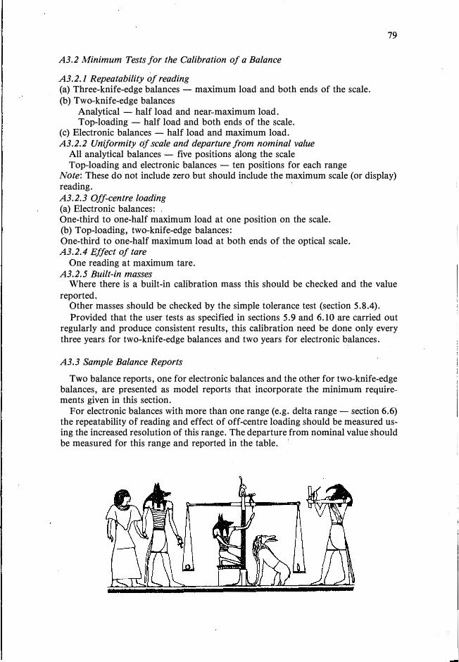
j;

I,

78

A2.3 Care of Masses

(a) When not in use the masses should always be kept in the box or container provid­ed.(b) Masses from two or more sets should never be mixed.(c) Masses should never be dropped; they should be placed on the pan or a clean sur­face.( d) Masses should never be placed on a dusty or dirty surface, or slid across a sur­face.(e) Masses should not be allowed to clink together. Sometimes it is necessary forthem to touch when using a number on a pan, but this should be done carefully. (f) If the masses appear dirty they should be dusted with a soft brush or lightlywiped with a clean chamois. If they still appear dirty they should be returned forcalibration.(g) Masses should never be cleaned with solvent.

APPENDIX 3. Minimum Requirements for Balance Reports

This appendix gives guidance as to which properties of the balance should be tested and how many readings made. Obviously a compromise has to be struck bet­ween usefulness and the cost of the measurements.

The following sections specify the minimum number of readings and types of tests that should be done on a balance for the calibration to be useful to the user. The specifications refer to all types of balances unless it is stated otherwise.

A3.J Number of Readings

Except for the repeatability a reading is defined as the symmetrical set: zero scale reading scale reading zero

A3.l.l Repeatability Ten readings at each position and load. Here a reading is (scale reading - zero).

A3.J.2 Sensitivity and scale value Two readings - except for two-pan balances where the sensitivity is measur­ed for each load and one determination is sufficient.

A3. J .3 One set of readings for each of the following tests: Uniformity of scale Departure from nominal value Effect of tare Off-centre loading Ratio of arms Parallelism of knife edges Hysteresis

A3,J.4 Calibration of masses Built-in calibration masses - twice Tolerance tests on masses - once

A3.2 Minimum Tests for the Calibration of a Balance

A3.2.l Repeatability of reading (a) Three-knife-edge balances - maximum load and both ends of the scale.(b) Two-knife-edge balances

Analytical - half load and near-maximum load.Top-loading - half load and both ends of the scale.

(c) Electronic balances - half load and maximum load.A3.2.2 Uniformity of scale and departure from nominal value

All analytical balances - five positions along the scale Top-loading and electronic balances - ten positions for each range

79

Note: These do not include zero but should include the maximum scale (or display) reading. A3.2.3 Off-centre loading (a) Electronic balances:One-third to one-half maximum load at one position on the scale.(b) Top-loading, two-knife-edge balances:One-third to one-half maximum load at both ends of the optical scale. A3.2.4 Effect of tare

One reading at maximum tare. A3.2.5 Built-in masses

Where there is a built-in calibration mass this should be checked and the value reported.

Other masses should be checked by the simple tolerance test (section 5.8.4). Provided that the user tests as specified in sections 5.9 and 6.10 are carried out

regularly and produce consistent results, this calibration need be done only every three years for two-knife-edge balances and two years for electronic balances.

A3.3 Sample Balance Reports

Two balance reports, one for electronic balances and the other for two-knife-edge balances, are presented as model reports that incorporate the minimum require­ments given in this section.

For electronic balances with more than one range (e.g. delta range - section 6.6) the repeatability of reading and effect of off-centre loading should be measured us­ing the increased resolution of this range. The departure from nominal value should be measured for this range and reported in the table.

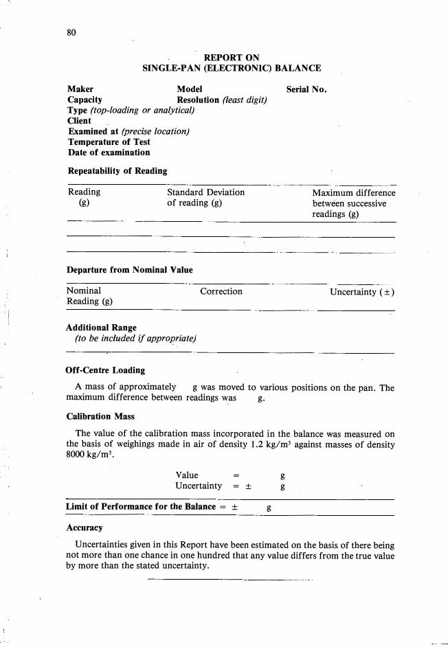
,1 1-I

:11: ji': I!: ii I ii ii

ii

80

REPORT ON SINGLE-PAN (ELECTRONIC) BALANCE

Maker Model Capacity Resolution (least digit) Type (top-loading or analytical) Client Examined at (precise location) Temperature of Test Date of examination

Repeatability of Reading

Reading (g)

Standard Deviation of reading (g)

Departure from Nominal Value

Nominal Reading (g)

Additional Range (to be included if appropriate)

Off-Centre Loading

Correction

Serial No.

Maximum difference between successive readings (g)

Uncertainty ( ±)

A_mass o� approximately g was moved to various positions on the pan. Themaximum difference between readings was g.

Calibration Mass

The value of the calibration mass incorporated in the balance was measured on the basis of weighings made in air of density 1.2 kg/m3 against masses of density 8000 kg/m3

•

Value g Uncertainty = ± g

Limit of Performance for the Balance = ± g

Accuracy

Uncertainties given in this Report have been estimated on the basis of there being not more than one chance in one hundred that any value differs from the true value by more than the stated uncertainty.

Notes

1. The balance has been tested according to the specifications laid down inThe Calibration of Balances

David B. Prowse CSIRO National Measurement Laboratory

81

2. When the sign of the correction is positive ( +) the amount should be added to thescale reading to give the correct value and when negative ( - ) subtracted from it.3. Air buoyancy corrections should be calculated on the basis that the object beingweighed is balanced against a hypothetical mass of density 8000 kg/m3 in air ofmeasured density.4. The Limit of Performance is the tolerance band within which all readings of thebalance will fall.

Remarks

(Any suitable statement of fact about the balance, its environment, or reference to

a covering letter may be made.)

Signature

Serial No.: Date:

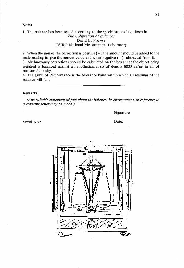
80

REPORT ON SINGLE-PAN (ELECTRONIC) BALANCE

Maker Model Capacity Resolution (least digit) Type (top-loading or analytical) Client Examined at (precise location) Temperature of Test Date of examination

Repeatability of Reading

Reading (g)

Standard Deviation of reading (g)

Depal'ture from Nominal Value

Nominal Reading (g)

Additional Range (to be included if appropriate)

Off-Centre Loading

Correction

Serial No.

Maximum difference between successive readings (g)

Uncertainty ( ±)

A. mass o� approximately g was moved to various positions on the pan. The maximum difference between readings was g.

Calibration Mass

The value of the calibration mass incorporated in the balance was measured on the basis of weighings made in air of density 1.2 kg/m3 against masses of density 8000 kg/m3.

Value Uncertainty = ±

Limit of Performance for the Balance = ±

Accul'acy

g

g

g

Uncertainties given in this Report have been estimated on the basis of there being not more than one chance in one hundred that any value differs from the true value by more than the stated uncertainty.

Notes

1. The balance has been tested according to the specifications laid down inThe Calibration of Balances

David B. Prowse CSIRO National Measurement Laboratory

81

2. When the sign of the correction is positive ( +) the amount should be added to thescale reading to give the correct value and when negative ( - ) subtracted from it.3. Air buoyancy corrections should be calculated on the basis that the object beingweighed is balanced against a hypothetical mass of density 8000 kg/m3 in air ofmeasured density.4. The Limit of Performance is the tolerance band within which all readings of thebalance will fall.

Remarks

(Any suitable statement of fact about the balance, its environment, or reference to a covering letter may be made.)

Signature

Serial No.: Date:

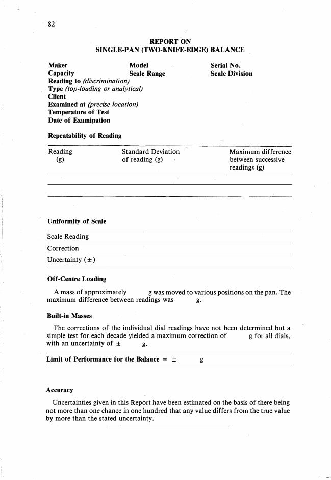
82

REPORT ON SINGLE-PAN (TWO-KNIFE-EDGE) BALANCE

Maker Model Capacity Scale Range Reading to (discrimination) Type (top-loading or analytical) Client Examined at (precise location) Temperature of Test

Date of Examination

Repeatability of Reading

Reading (g)

Uniformity of Scale

Scale Reading

Correction

Uncertainty ( ±)

Off-Centre Loading

Standard Deviation of reading (g)

Serial No. Scale Division

Maximum difference between successive readings (g)

A mass of approximately g was moved to various positions on the pan. The maximum difference between readings was g.

Built-in Masses

The corrections of the individual dial readings have not been determined but a simple test for each decade yielded a maximum correction of g for all dials, with an uncertainty of ± g.

Limit of Performance for the Balance = ± g

Accuracy

Uncertainties given in this Report have been estimated on the basis of there being not more than one chance in one hundred that any value differs from the true value by more than the stated uncertainty.

Notes

1. The balance has been tested according to the specifications laid down inThe Calibration of Balances

David B. Prowse CSIRO National Measurement Laboratory

83

2. When the sign of the correction is positive ( +) the amount should be added to thescale reading to give the correct value and when negative ( - ) subtracted from it.3. Air buoyancy corrections should be calculated on the basis that the object beingweighed is balanced against a hypothetical mass of density 8000 kg/m3 in air ofmeasured density.4. The Limit of Performance is the tolerance band within which all readings of thebalance will fall.

Remarks

(Any suitable statement of fact about the balance, its environment, or reference to a covering letter may be made.)

Signature

Serial No.: Date:

------------------gq

82

REPORT ON SINGLE-PAN (TWO-KNIFE-EDGE) BALANCE

Maker Model Capacity Scale Range Reading to (discrimination) Type (top-loading or analytical) Client Examined at (precise location) Temperature of Test Date of Examination

Repeatability of Reading

Reading (g)

Uniformity of Scale

Scale Reading

Correction

Uncertainty ( ± )

Off-Centre Loading

Standard Deviation of reading (g)

Serial No. Scale Division

Maximum difference between successive readings (g)

A mass of approximately g was moved to various positions on the pan. The maximum difference between readings was g.

Built-in Masses

The corrections of the individual dial readings have not been determined but a simple test for each decade yielded a maximum correction of g for all dials, with an uncertainty of ± g.

Limit of Performance for the Balance

Accuracy

± g

Uncertainties given in this Report have been estimated on the basis of there being not more than one chance in one hundred that any value differs from the true value by more than the stated uncertainty.

Notes

1. The balance has been tested according to the specifications laid down inThe Calibration of Balances

David B. Prowse CSIRO National Measurement Laboratory

83

2. When the sign of the correction is positive (+)the amount should be added to thescale reading to give the correct value and when negative ( - ) subtracted from it.3. Air buoyancy corrections should be calculated on the basis that the object beingweighed is balanced against a hypothetical mass of density 8000 kg/m3 in air ofmeasured density.4. The Limit of Performance is the tolerance band within which all readings of thebalance will fall.

Remarks

(Any suitable statement of fact about the balance, its environment, or reference to

a covering letter may be made.)

Signature

Serial No.: Date: