the building science of office surfaces: … · ii the building science of office surfaces:...
TRANSCRIPT

THE BUILDING SCIENCE OF OFFICE SURFACES:
IMPLICATIONS FOR MICROBIAL COMMUNITY
SUCCESSION
by
Mahnaz Zare
A thesis submitted in conformity with the requirements
for the degree of Master of Applied Science
Civil Engineering
University of Toronto
© Copyright by Mahnaz Zare (2015)

ii
THE BUILDING SCIENCE OF OFFICE SURFACES:
IMPLICATIONS FOR MICROBIAL COMMUNITY SUCCESSION
Mahnaz Zare
Master of Applied Science
Civil Engineering
University of Toronto
2015
Abstract
The Surface Project studied the microbial succession on office surfaces in nine offices in three
North American cities. Building science parameters including relative humidity (RH),
temperature, equilibrium relative humidity (ERH), illumination, and occupancy were measured to
investigate their impact on microbial communities. Parameters were measured every five minutes
over the course of a year. ERH, RH, temperature, occupancy, and illumination varied between
offices, and cities which suggests that building characteristics and climate are important factors.
RH, ERH, and temperature showed clear seasonal variation. The drywall ERH varied from ERH
of ceiling tile and carpet and from the RH of air. Illumination was different in occupied and
unoccupied offices. Occupancy did not cause that much difference in RH. Methodology analysis
revealed no difference between different frequency measurements, although it is suggested that
short-term intervals to be considered since long-term intervals may not show the large variation of
building science parameters.

iii
Acknowledgments
I would like to thank my supervisor, Dr. Jeffrey Siegel for giving me the opportunity to be involved
in this research, and for his guidance and patience throughout the project. I would like to
acknowledge Alfred P. Sloan foundation, Dr. Greg Caporaso, Dr. Scott Kelley, and Dr. Rob Knight
for being wonderful collaborators. I thank Dr. Kim Pressnail for accepting to be the second reader.
I also thank staff at the University of Toronto, Northern Arizona University, San Diego State
University, and Argonne National Laboratory for accommodating the research and for providing
assistance throughout the project.
I would like to thank John Chase, Jennifer Fouquier, Sandra Dedesko, and Dylan McTavish for
their extensive help in data collection, microbial sampling, and support.
I thank my husband, close family, and friends for their continued encouragement. I dedicate this
work in memory of my father and sister. I miss them every day; however they were along, with
my mother, husband and all my family, incredible supporters through all the years.

iv
Table of Contents
Abstract ........................................................................................................................................... ii
Acknowledgments.......................................................................................................................... iii
Table of Contents ........................................................................................................................... iv
List of Tables ................................................................................................................................ vii
Table of Figures ........................................................................................................................... viii
List of Abbreviations ..................................................................................................................... xi
Chapter 1 Objectives and Literature Review ...................................................................................1
Introduction ..........................................................................................................................1
Objectives ............................................................................................................................3
Literature review ..................................................................................................................5
1.3.1 Impact of moisture, temperature, and illumination ..................................................7
1.3.2 Variation of microbial community within and across buildings and regions ........10
1.3.3 Seasonal variation of microbial communities ........................................................13
1.3.4 Impact of human occupancy on microbial communities .......................................15
1.3.5 Summary ................................................................................................................17
Chapter 2 Methodology .................................................................................................................19
Summary ............................................................................................................................19
Selection of offices and cities ............................................................................................19
Selection of materials .........................................................................................................20
Description of offices in each city .....................................................................................20
Description of sensors ........................................................................................................22
Detailed apparatus ..............................................................................................................23
Data management and organization ...................................................................................24

v
Microbial sampling and sequencing ..................................................................................26
Calibration of sensors ........................................................................................................27
Calibration procedure.........................................................................................................27
Chapter 3 Results ...........................................................................................................................29
Research question 1: What is the range of hygrothermal conditions in the buildings? .....30
3.1.1 Range of equilibrium relative humidity and air relative humidity ........................30
3.1.2 Time of wetness .....................................................................................................32
3.1.3 Range of near surface temperature and air temperature ........................................35
Research question 2: How do air relative humidity and equilibrium relative humidity, temperature, occupancy, and illumination vary within offices? ........................................37
3.2.1 Variation of ERH and RH within offices ...............................................................37
3.2.2 Variation of temperature within offices .................................................................39
3.2.3 Variation of illumination within offices ................................................................41
Research question 3. How do relative humidity, equilibrium relative humidity, temperature, and illumination vary between offices? ........................................................43
3.3.1 Variation of ERH and RH between offices ............................................................43
3.3.2 Variation of temperature between offices ..............................................................44
3.3.3 Variation of occupancy between offices ................................................................44
3.3.4 Variation of illumination between offices .............................................................45
Research question 3: How does the surface moisture of various materials differ from one another and from RH of air? .......................................................................................46
3.4.1 Difference between ERH of materials ...................................................................46
3.4.2 Difference between ERH and RH ..........................................................................47
Research question 4: How do relative humidity, equilibrium relative humidity, temperature, and illumination vary in different seasons and months?...............................49
3.5.1 Variation of moisture over seasons and months ....................................................49
3.5.2 Variation of temperature over seasons and months ...............................................54

vi
3.5.3 Variation of illumination over seasons and months ...............................................58
3.5.4 Variation of occupancy over seasons and months .................................................60
Research question 5: Do short-term intervals show the variation in building science parameters? Do the current measurements show the impact of past data measurements? ...................................................................................................................61
3.6.1 Frequency of measurement ....................................................................................61
3.6.2 History of moisture parameters ..............................................................................63
Chapter 4 Discussion .....................................................................................................................65
Chapter 5 Conclusion .....................................................................................................................74
Chapter 6 Bibliography .................................................................................................................75
Appendix A ....................................................................................................................................85
The location of each plate in each office ..................................................................................85
Appendix B ....................................................................................................................................86
Calculation of calibration and collocation coefficients .............................................................86
Appendix C ....................................................................................................................................87
Calibration and collocation coefficient .....................................................................................87
Appendix D ....................................................................................................................................89
Seasonality of ERH, RH, and temperature in Office 2 and 3 ...................................................89
Appendix E ....................................................................................................................................92
Outdoor average temperature ....................................................................................................92

vii
List of Tables
Table 1. Size, occupancy and orientation of windows in each office in Flagstaff, San Diego, and
Toronto .......................................................................................................................................... 21
Table 2. Characteristics of Sensors ............................................................................................... 23
Table 3. Percentage of missing data points in Flagstaff, San Diego, and Toronto ....................... 26
Table 4. Uncertainty of calibration under ideal conditions ........................................................... 27
Table 5. The maximum and mean hours above the threshold values of 60%, 65%, and 70% for
ERH of drywall and RH of air on the wall plate in nine offices in Flagstaff, San Diego, and
Toronto .......................................................................................................................................... 34
Table 6. Correlation coefficient between near surface temperature of drywall and ERH of
drywall and correlation coefficient between air temperature and RH on the wall plate in nine
offices ............................................................................................................................................ 73

viii
Table of Figures
Figure 1. The apparatus used on every surface at every site. Wall plates had ERH sensors in all
sites. Floor and ceiling ERHs were measured for drywall only at one site in each of the three
cities. ............................................................................................................................................. 24
Figure 2. Range and frequency distribution of ERH of materials (Dr=drywall, Ce= ceiling tile,
Ca= carpet tile) and RH of air on the wall plate in nine offices in Flagstaff (top), San Diego
(middle), and Toronto (bottom) .................................................................................................... 31
Figure 3. ERH of materials and RH of air on the wall plate in Office 1 in Toronto during a 24-
hour period on August 1st, 2013 .................................................................................................... 32
Figure 4. Time of wetness for ERH of drywall and RH of air on the wall plate on August 1st,
2013 in T2 (left) and T3 (right) in Toronto ................................................................................... 33
Figure 5. Total time of wetness for ERH of drywall and RH of air on the wall plate between
offices in Flagstaff, San Diego, and Toronto ................................................................................ 34
Figure 6. Range and frequency distribution of near surface temperature of materials (Dr=drywall,
Ce=ceiling tile, Ca=carpet tile) and air temperature on the wall plate in nine offices in Flagstaff
(top), San Diego (middle), and Toronto (bottom)......................................................................... 36
Figure 7. Air temperatures and the near surface temperatures of drywall, carpet and ceiling tile
on the wall plate in Office 3 in Toronto on March 1st 2014 ......................................................... 37
Figure 8. Range and frequency distribution of ERH of drywall and RH of air between ceiling,
floor, and wall in Office 1 in Flagstaff (top), and San Diego (middle) and Office 3 in Toronto
(bottom)......................................................................................................................................... 38
Figure 9. Range and frequency distribution of near-surface temperature of drywall and air
temperature between ceiling, floor, and wall in Office 1 in Flagstaff (top) and San Diego
(middle), and Office 3 in Toronto (bottom) .................................................................................. 40

ix
Figure 10. Air temperature on ceiling, floor, and wall in Office 1 (left) and 2 (right) in Toronto
on July 16th, 2013 .......................................................................................................................... 41
Figure 11. Range and median illumination on floor, ceiling, and wall in nine offices in Flagstaff
(top), San Diego (middle), and Toronto (bottom)......................................................................... 42
Figure 12. Variation of occupancy over the course of a year between nine offices in Flagstaff,
San Diego, and Toronto ................................................................................................................ 45
Figure 13. Percent difference of equilibrium relative humidity (ERH) from air relative humidity
(RH) for Dr= Drywall, Ce=ceiling tile and Ca=carpet tile samples in all nine offices in Flagstaff
(top), San Diego (middle), and Toronto (bottom)......................................................................... 48
Figure 14. Seasonal variation of ERH of drywall (left) and RH of air (right) on the wall plate in
Office 1 in Flagstaff (top), San Diego (middle), and Toronto (bottom) ....................................... 51
Figure 15. Monthly variation of ERH of drywall and RH of air on the wall plate in three offices
in Flagstaff (top), San Diego (middle) and Toronto (bottom) (starting from June 2013 to May
2014) ............................................................................................................................................. 53
Figure 16. Seasonality of air temperature on the wall plate in Office 1 in Flagstaff (top), San
Diego (San Diego), and Toronto (bottom) .................................................................................... 55
Figure 17. Monthly variation of temperature on the wall plate in nine offices in Flagstaff (top),
San Diego (middle), and Toronto (bottom) (starting from June 2013 to May 2014) ................... 57
Figure 18. Seasonality of illumination on the wall, ceiling, and floor in nine offices in Flagstaff
(top), San Diego (middle), and Toronto (bottom)......................................................................... 58
Figure 19. Monthly variation of illumination in nine offices on the wall plate in Flagstaff (top),
San Diego (middle), and Toronto (bottom) (starting from June 2013 to May 2014) ................... 59
Figure 20. Seasonal variation of occupancy sensor trigger fraction on the wall plate in nine
offices in Flagstaff, San Diego, and Toronto ................................................................................ 60

x
Figure 21. Monthly variation of occupancy sensor trigger fraction on the wall plate in nine
offices in Flagstaff, San Diego, and Toronto (starting from June 2013 to May 2014) ................. 61
Figure 22. Frequency of measurement for equilibrium relative humidity of drywall (left) and
illumination (right) on the wall plate in Office 1 in Toronto ........................................................ 62
Figure 23. Moving average of ERH and RH on the wall plate in Office 1 in Flagstaff (left), San
Diego (middle), and Toronto (right) ............................................................................................. 64
Figure 24. Illumination on the wall plate in unoccupied and occupied offices in Flagstaff, San
Diego, and Toronto ....................................................................................................................... 70
Figure 25. Air relative humidity on the wall plate in two situations, unoccupied and occupied
offices in Flagstaff, San Diego, and Toronto ................................................................................ 72

xi
List of Abbreviations
Ce Ceiling tile F1 Office 1 in Flagstaff
Ca Carpet tile F2 Office 2 in Flagstaff
Dr Drywall F3 Office 3 in Flagstaff
C Ceiling S1 Office 1 in San Diego
F Floor S2 Office 2 in San Diego
W Wall S3 Office 3 in San Diego
F Flagstaff T1 Office 1 in Toronto
S San Diego T2 Office 2 in Toronto
T Toronto T3 Office 3 in Toronto
RH Relative Humidity
ERH Equilibrium Relative Humidity
UV Ultraviolet

1
Chapter 1 Objectives and Literature Review
Introduction
Industrialization and urbanization has changed lifestyles and in developed countries, we spend
90% of our time in different indoor environments such as offices, homes, schools and workplaces
(Hoppe & Martinac, 1998). Indoor environments are also habitat for trillions of microorganisms
(Amend et al., 2010; Rintala et al., 2008) including bacteria, fungi, and viruses. Microbial
communities can be found everywhere: in indoor air, on surfaces we touch frequently such as door
handles or cellphones, and also on materials used in the construction of buildings. The indoor
microbiome originates from many sources including human occupancy (Hospodsky et al., 2012),
pets (Dunn et al., 2013), outdoor air (Meadow et al., 2013), and plants (Shibata et al., 2004).
Building design, relative humidity and temperature, air flow rate, and ventilation are factors that
affect diversity and composition of microbial communities (Kembel et al., 2012). However, it is
not yet known how these factors impact microbial communities indoors (Kembel et al., 2012). In
addition, studies have shown that due to the frequency of cleaning (Rusin et al., 1998), number of
occupants (Hospodsky, et al., 2012), and ventilation rate (Kujundzic et al., 2006) microbial
communities change within buildings in the same region, and microorganisms found in various
buildings can be very different (Dunn et al., 2013). Results of many investigations show that indoor
microbial communities are different from those found outdoors (e.g., Tringe et al., 2008; Amend
et al., 2010). Kembel et al. (2012) have shown that microbial communities in mechanically
ventilated hospital rooms are different from outdoor communities.
Microorganism have different functions: bacteria found in nature are responsible for recycling of
organic matter (Alongi, 1994) and fungal cells can sorb metals from dilute solutions (Huang et al.,
1990). However, exposure to indoor microorganisms can have positive or negative impacts on our
health, For example, molds can cause asthma in both infants (Jaakkola et al., 2010) and adults
(Karvala et al., 2010). There is controversy that exposure to indoor fungi can cause headaches,
fatigue, and difficulties in concentration, symptoms associated with Sick Building Syndrome
(Terr, 2009). However, there are also studies that suggest being exposed to microbial communities

2
in the early stage of life can protect humans from developing diseases later in life (e.g., Strachan,
1989; Iossifova et al., 2007).
Microorganisms can also have positive or negative impact on building materials. Warscheid (2000)
showed that nitric acid produced by nitrifying bacteria can degrade stones. In contrast, Gaylarde
et al. (2003) showed that existence of lichens (lichens are composite organisms consisting of fungi
and photosynthetic partners) can have a protective role against degradation of materials by black
fungi. Furthermore, restoration of buildings with serious and visible mold growth on materials is
a costly process. For example, remediation of mold growth on a large courthouse in Florida cost
approximately $45 million (NIOSH, 1993) and workers who are exposed to existing molds on the
building materials can experience health problems (NIOSH 1993).
Due to the importance of microorganisms and the role they play, it is essential to explore them.
However, due to the complexity of microbial communities such as the enormous number of
microorganisms in human body, 10 times more than human cells, (American Society for
Microbiology, 2008), on surfaces we touch frequently, e.g., 25,000 microorganisms per square
inch of cellphones (Calvan, 2010), we only have a small perspective on the indoor microbiome.
We also know relatively little about the time-scale change of microbial communities in the indoor
environment. Furthermore, buildings are different in design, building materials, contents,
occupancy, and ventilation. For example, office spaces are occupied usually for eight hours per
day, in contrast to homes, which are typically occupied for longer periods. In addition, the activities
done in homes are different from the activities done in offices, such as cooking and taking showers.
The differences between building science parameters (e.g., relative humidity, temperature,
illumination) may cause difference in microbial communities. Therefore, we need a richer
knowledge about the potential impact of building materials, environmental parameters, human
occupancy, climates, and seasons on the diversity and distribution of indoor microbial
communities. In addition to being scientifically compelling, a better understanding of indoor
microorganisms allows us to provide a healthy indoor environment, reduce degradation of building
materials, and reduce the potential costs associated with mold remediation and associated material
repair and replacement.

3
Objectives
Our rich understanding of the diversity and dynamics of indoor fungal and bacterial communities
is not commensurate with our knowledge of building science parameters and how they influence
the indoor microbiome. Lack of environmental data may result in incomplete knowledge about
how microbial communities change in various indoor environments (Corsi et al., 2012). In
addition, researchers have rarely investigated the indoor microbial communities simultaneously
with building science parameters to determine how typical building science parameters affect the
accumulation of microorganisms on building materials. Furthermore, there is a need for further
investigation of indoor microbial communities during various seasons simultaneously with
investigation of building science parameters such as relative humidity and temperature. We need
to know if building science parameters vary within and between buildings in a way that
meaningfully affects microbial communities.
We know from the literature that moisture is an important factor in proliferation of
microorganisms. Moisture can be available to microorganisms through relative humidity, moisture
content, and condensed and bulk moisture on the surface of materials. There are studies (e.g.,
Pasanen et al., 2000; Nielsen et al., 2004) that have investigated the moisture requirements of
microbial communities particularly in conditions with high relative humidity. However, there is a
need for further investigation of surface moisture of different materials, and how surface moisture
changes over time. We also need to know if there is a significant difference between surface
moisture and relative humidity.
To address these issues, this thesis investigates the impact of materials, buildings, climates, and
seasons on building science measurements including temperature, equilibrium and air relative
humidity, illumination, and occupancy. These results are part of a larger project investigating how
these parameters affect microbial communities. In addition to the building science parameters
described herein, there has been a coincident extensive campaign of microbial sampling. The
investigation occurred in nine offices in three North American cities with different climates:
Flagstaff (Arizona), San Diego (California), and Toronto (Ontario). The overall objective for the
project is to study the impact of climate on building science metadata in indoor environments, and
to study the impact of building materials on surface moisture on different surfaces and in different

4
buildings. The project also investigates the impact of human occupancy, climate and building
materials on the microbial succession, patterns in the establishment of microbial community in the
built environment, and the nature and rate of community change over time.
The literature review (discussed in Section 1.3) shows that microbial communities might be
different between different locations due to occupancy, occupant behavior, building materials, and
indoor environmental conditions. Based on these facts and in this thesis, the hypotheses are:
differences in climate and building design cause environmental parameters (air relative humidity
and equilibrium relative humidity, temperature, illumination) to vary within and across cities and
buildings. In addition, seasons cause variation in environmental parameters, and long-term
measurements are necessary to determine the variations in parameters. Based on these hypotheses,
the research questions addressed by this thesis are listed below
1. What is the range and dynamics of hygrothermal (including relative humidity, equilibrium
relative humidity, and temperature) conditions in the studied buildings? The literature
suggests that microbial communities proliferate in conditions with high moisture: how
frequently do the extreme conditions occur in the test environments?
2. In addition to extreme conditions, we need to investigate the building science parameters
on different surfaces including ceiling, wall, and floor in the test offices. How do the
building parameters (air relative humidity and equilibrium relative humidity, temperature,
and illumination) change within offices?
3. The test offices have different design, ventilation operation, occupancy schedules, and
surface finishes and construction materials. How do the building science parameters vary
across the test offices?
4. Besides the building science parameters, material type is another potential factor affecting
both the accumulation of microbial communities and surface moisture of materials. How
does the surface moisture on various materials differ from one another? Materials studied
in the project, vary in their properties (e.g., composition, porosity) and this difference might
affect the surface moisture of selected material. The literature suggests that the surface

5
moisture of materials is an important factor affecting microbial communities (e.g.,
Flannigan and Morey, 1996; Pasanen et al., 2000).
5. Finally, the frequency and period of measurement needs investigation. Do short-term
intervals show the variation in building science parameters that is revealed by the year-
long measurements in this project? Do short-term measurements reveal the impact of past
moisture problems? The majority of published papers investigated the microbial
communities during short-term periods.
This thesis first reviews the research in the field of indoor microbial communities and shows the
need for further investigation of building science data collection in previous studies. The work
then describes the long-term data collection methodology, site selection, and calibration of
equipment. The measured parameters included relative humidity, temperature, equilibrium relative
humidity and near surface temperature of selected materials, illumination, and human occupancy
in nine offices in three North American cities. The parameters were measured every 5 minutes
over a course of a year from May 2013 to May 2014 in San Diego, June 2013 to May 2014 in
Flagstaff, and July 2013 to May 2014 in Toronto. Although the microbial samples are still being
sequenced, building science measurements in conjunction with microbial sampling provides a
better insight into the impact of building parameters on indoor microbial communities. If building
science parameters change between offices, seasons, and if surface moisture of materials differ
from one another, it is expected that a variation in microbial communities between buildings,
seasons, and on test materials will be seen. Finally, the building science parameters and microbial
sampling results will help us to decide which materials are more susceptible to the accumulation
of microorganisms in different climates.
Literature review
The built environment is an important habitat for humans. Microorganisms are also important
inhabitants of the indoor environment and are often different from those found outdoors. The
interaction between the microbial communities, humans, and other indoor pollutant sources might
affect human health. Building materials and design, and climate are all factors that could affect the
growth of microorganisms. Therefore, it is necessary to explore indoor microbial communities and
their relationship to the built environment (Kelley & Gilbert, 2013).

6
The investigation of microbial communities has evolved over the past decades. Culturing is one
way of investigating the communities. In this method, the microbial organisms reproduce in a
culture media on agar plates under controlled conditions. Thousands of culture-based studies have
shown that built environments are occupied by microbes. Furthermore, culture-based
investigations allow the study of the environmental factors that are necessary for survival of
communities. However, this method is limited to particular microorganisms that culture well
(Anaissie et al., 2002), and further invetigation of built environments reveals organisms that are
not culturable (Amann et al., 1995). Using culture-independent approaches, such as DNA
sequencing, has revealed previously unreported and diverse microorganisms (Hugenholtz et al.,
1998). This method can extract DNA from the cells in a sample and amplify the extracted genes
(Tringe & Hugenholtz, 2008). The culture-independent technology has improved in terms of
speed, cost, and accuracy, which enables the technology to analyze a broader range of samples
simultaneously. The improvements help to discover the impact of humans and other sources on
the built environment, and how microbial communities are changing in the built environment
(Hugenholtz et al., 1998).
The collaboration of microbiologists with building scientists provides a broader perspective on the
built environment, since environmental conditions and buildings materials play an important role
in providing the favourable conditions for growth and proliferation of microorganisms (Kelley &
Gilbert, 2013). In addition, fungi are different from bacteria regarding their reaction to seasonality,
human impact, and location. Immigration of outdoor fungi to indoors is an important source of
indoor fungi (Adams et al., 2013). Geographical location and seasons are also the most important
factors affecting indoor fungi (Amend et al., 2010). In contrast, bacteria are affected by humans
and their activities and there is no clear seasonality trend of bacteria (Adams et al., 2014;
Hospodsky et al., 2012). Therefore, there is a need for in-situ studies that investigate indoor
microbial communities simultaneously with building science parameters including temperature,
moisture and illumination, geographical location, occupancy, and seasonality. The following
sections will review the projects that have investigated these parameters, their impact on indoor
microbial communities, and variation of microbial communities within and between the buildings.
The articles described in this chapter are selected based on the research questions described in
Section 1.2. If previous investigations show that microbial communities change within and

7
between the buildings, we would expect to observe the variation of building science parameters
between and within the test offices. In addition, the literature review will help us to determine and
investigate which subjects have not been investigated in previous studies, such as the frequency of
measurement of building science parameters.
1.3.1 Impact of moisture, temperature, and illumination
Moisture damage has always been an issue in buildings since wet materials can support fungal and
bacterial growth, and moisture often accelerates material deterioration (Flannigan et al., 1996) and
can cause health problems for occupants (Dales et al., 1991; Peat et al., 1998). Moisture and
nutrients present on materials impact the microbial communities, although the effect can vary due
to the difference in material composition, and moisture content. In addition, deposited soil or dirt
on the surface of used materials is another factor affecting the water absorption of materials (West
& Hansen, 1989).
Moisture is one of the primary factors affecting the proliferation of microbial communities (Grant
et al., 1989). The state of moisture in materials is expressed in several ways, such as moisture
content and water activity. Moisture content is defined as the volumetric fraction (m3/m3) or mass
fraction (kg/kg) of water in the material. The water activity is the ratio of vapor pressure of water
in a material to the vapor pressure of pure water at the same temperature. The relative humidity
(RH) above the surface of a material in an equilibrium condition is called equilibrium relative
humidity (ERH) and is equivalent to water activity only at equilibrium conditions. One of the early
studies that investigated the impact of water activity on fungal growth was conducted by Ayrest
(1969). The author studied the effect of water activity and temperature on twelve species of fungi
using culture-based method on the agar medium in glass tubes. Germination and growth rate of
species were monitored during intervals of 12 hours and 16 days. Species showed different
behavior regarding water activity and temperature requirements. The investigation revealed that if
water activity is low, a higher temperature is needed to activate growth. Although the results
suggest that both temperature and water activity should be investigated simultaneously, the study
only considered a limited number of species and also building materials were not studied. Pasanen
et al. (2000) conducted an experiment in various wetting and drying conditions using wood board,
particle board, and gypsum board in the laboratory. They investigated the impact of absorption of

8
water through direct water damage, and surface condensation. After each wetting stage, a drying
stage was also conducted at different temperatures and relative humidity. The difference between
RH and temperature at different stages of wetting and drying conditions resulted in different
moisture contents and ERHs in materials. Some fungal spores were adapted to the fluctuating
wetting and drying environments and could survive the second drying period. The study confirmed
the results of previous studies (e.g., Flannigan and Morey, 1996) that the paper on the gypsum
board has a different capacity for sorption of water and it is necessary to consider its impact on the
bulk material. The authors suggested that the presence of fungal communities on the surface of
materials was due to the moisture on the surface of material (water activity) and it is essential to
consider this parameter in investigations. Further investigation of water activity revealed the
importance of this parameter. For example, Nielsen et al. (2004) assessed fungal growth on 21
materials at different ERH values (also called water activity in their paper because the test
chambers were at equilibrium) in laboratory chamber experiments and found positive associations
between ERH and fungal growth. However, it should be noted that these studies were short-term
and in-situ conditions were not investigated. In addition, the investigations focused on extreme
moisture conditions and typical RH and ERH remains largely unexplored.
Although moisture is a key factor affecting fungal growth, the amount of time that moisture is
available is also important. Adan (1994) introduced the term “time of wetness” and it is “fraction
of times that relative humidity near the surface of material is above the threshold value of 80%”.
He showed that growth of Penicillium on both bare and coated gypsum is a function of time of
wetness. Adan (1994) also showed that even a thin layer of surface condensation for a short time
(e.g., during showering) may act as a moisture reservoir and prolong time of wetness.
Temperature has been also shown to affect microbial communities. For purposes of describing
growth, temperature can be divided into lower limit, upper limit, and optimum temperature for
growth (Morita, 1975). The lower and upper limit may damage the cellular component and
membrane of microbial communities (Nedwell, 1999). For example, temperatures higher than
24°C will reduce the survival of airborne bacteria such as E.coli (Handley & Webster, 1995), and
Salmonella (Dinter and Moller, 1998). However, Nedwell, (1999) suggests that some species may
adapt to the temperature variation. Further investigation of the effect of temperature on the
microbial communities revealed positive correlation between temperature and concentrations of

9
indoor fungi in Danish homes (Frankel et al., 2012). The same results were observed in homes in
the Northeast of the USA (Reponen et al., 1992). In contrast, indoor concentrations of bacteria
were negatively correlated with indoor temperature both in Danish (Frankel et al., 2012) and
Cincinnati homes (Green et al., 2003). Although the investigation done by Frankel et al. (2012)
explains the relationship between temperature and microbial communities, they measured indoor
temperature only on the day of sampling for 15 minutes in the morning and the history of past
temperature was not provided. Therefore, it is hard to conclude how or if the past temperature
affects the microbial communities. In this thesis we will analyze the history of the measured
building science parameters to determine how spot measurements are different when compared to
historical data.
Material type is another factor affecting fungal growth. Ceiling tile is a commonly used material
in commercial and institutional buildings (Chang et al., 1995). Chang et al. (1995) assessed the
moisture content and impact of four different types of ceiling tile on the fungal growth in static
chambers with relative humidity in the range of 54 to 97%. Three of the ceiling tiles were new,
and one was 10 years old. The used ceiling tile had the same characteristics (fire rating, washable,
standard white) as one of the new tiles. The results showed that the used ceiling tile had higher
moisture content and ERH compared to the new ones, and was also more susceptible to fungal
growth. Higher susceptibility may be due to the existence of dust on the material that is providing
the nutrients for fungal growth. The results revealed that different ceiling tiles need different ERH
to support fungal growth, although there is a need for in-situ experiments to investigate the impact
of indoor environmental conditions such as temperature and location on ERH.
Early studies also reported that sunlight is another factor affecting growth of bacterial communities
(Downes & Blunt, 1877; Koch, 1890; Hochberger, 2000). Koch (1890) revealed that sunlight can
kill bacteria in a few minutes to several hours behind glass. Later investigations showed that the
survival of bacterial communities depend on the thickness of communities exposed to sunlight
(Solly, 1897) and type of glass (Smith, 1942), since the disinfection effect of sunlight is reduced
by some glass (Chapple et al., 1992). Unfortunately, sunlight effects have not been investigated
recently, although there are some studies that have investigated the effect of artificial
(Buchbinder et al., 1941) and ultraviolet light (Kowalski, 2009). The UV technology is an
emerging method to lessen the transmission of microorganisms that cause severe health effects.

10
Recently a number of studies have investigated the disinfection effect of UV. However, some
contradictory results about the disinfection ability of sunlight and UV have been observed because
the impact of UV or sunlight may change in different RH levels. For example, Lidwell and
Lowbury (1950) investigated the effect of sunlight on the disinfection of airborne flora and
demonstrated that higher RH improves the disinfection. The same results was obtained for
disinfection of bacteria using UV (Riley and Kaufman, 1972). In contrast, Peccia et al. (2011) and
Ko et al. (2000) showed that Rh higher than 85% decreased the inactivation rate of UV. Due to the
lack of information about illumination effect and the impact it may have on microbial
communities, the current thesis is investigating variation of illumination in the test offices.
Overall, the investigations showed that temperature, moisture, and sunlight are important factors
for the survival and/or growth of microbial communities. Material type is also an important feature
affecting the moisture content and the moisture on the surface of materials. In addition, older
materials are different from the new ones in their moisture content and need further investigation.
However, these investigations were short-term and occurred in laboratories. Therefore, long-term
and in-situ conditions remain unexplored and are addressed in parts in this thesis.
1.3.2 Variation of microbial community within and across buildings and regions
Building design, function of spaces (Kembel, et al., 2014), and geographical location (Lighthart &
Stetzenbach, 1994; Shaffer & Lighthart, 1997) are likely factors affecting microbial communities.
Even samples collected from the same location can change across time (Lighthart & Stetzenbach,
1994). In addition to the temporal variation, ‘The first law of geography’ suggests that increasing
the distance between two observations declines the similarity between them (Tobler, 1970). This
phenomena is called spatial variation. There are studies that investigated the spatial differences of
microbial communities locally and globally. Amend et al. (2010) investigated the indoor fungal
communities globally to determine if there is relationship between fungal composition and
dispersal limitation (i.e., there are some factors such as environmental conditions that may limit
the distribution of species over a larger spatial scale). They used culture independent technologies
for DNA sequencing of dust samples collected from different buildings. According to the results,
fungal communities from the same location were similar regarding genetic evolution. The results
showed more diverse fungal communities in the regions with temperate climate than in the tropical

11
countries, and the distance from the equator was a good parameter for differentiating the genetic
similarity of fungal communities. Despite the distinct difference between buildings within a
region, there was a significant similarity between regional fungal samples. The authors suggest
that the reason might be the strong effect of the outdoor environment; however, the investigation
did not consider the indoor environmental conditions such as RH or temperature.
Also on a local scale, Adams et al. (2013) and (2014) studied the composition of indoor and
outdoor airborne fungi and bacteria and their dispersal pattern in residential buildings free of water
damage and mold problems. They collected dust samples from the surface of sterilized empty
dishes that were suspended from ceiling. Samples were DNA sequenced for investigation of fungi
and bacteria. The results showed that community richness was higher outdoors than indoors.
Outdoor fungal communities were different from indoor communities and more fungal biomass
was detected outdoor. The results revealed that the richness of bacterial communities was not
significant between the rooms within a building, although bacterial richness varied across the
buildings and was higher in buildings with a humidifier. By increasing the indoor distance from
outdoors within a unit, the similarity between indoor and outdoor fungal communities decreased,
and the bacterial communities on the entryway of rooms (with a smaller distance from outdoor)
were similar to the outdoor. For bacterial communities, a greater difference was found between
samples that were farther from each other in space than closer samples. While room type (floor
level) and unit were the parameters affecting the bacteria, unit and geographical distance affected
the fungal communities significantly. Although both studies provide information about the
dispersal pattern of airborne microbial communities, there is a need to investigate if the dispersal
pattern of microbial communities will be observed on building materials on different locations
such as floors or ceilings. Furthermore, it is necessary to investigate how temperature and RH
affect the dispersal pattern of microbial communities.
Variation of microbial communities between buildings is another phenomena that has been
explored. For example, Tsai & Macher (2005) investigated the bacterial communities in 100 office
buildings (including non-problem and problem buildings) mostly located in urban areas across the
USA using culture-based methods. They collected dust samples from three random sites within
each building either in winter or summer. The results showed that the ratio of indoor to outdoor
bacterial concentrations was different between offices. For example, the ratio of indoor to outdoor

12
bacterial concentrations were less than one in 65% of the buildings, while in the remaining
buildings the ratio was higher than one. Aggregated concentrations of bacteria within the buildings
were moderately correlated together, although there were differences between absolute
concentrations of bacteria within sites. This study investigated the office buildings in different
climatic zones across the USA either in winter or summer; however buildings were not
investigated in both seasons, and within the buildings a limited number of samples were collected.
In addition, the effect of environmental conditions on the microbial communities were not studied.
Further local investigation of bacterial and fungal communities also showed the variation of
microbial communities within and between buildings. For example, Flores et al. (2013)
investigated the bacterial communities on various surfaces in the kitchens of four residential
buildings using DNA sequencing. The results showed that within the kitchens, communities were
more similar, although across the kitchens greater differences were observed. The authors suggest
that the difference between materials and environmental conditions are the probable cause of the
difference. The results are in good agreement with other studies such as (Rintala et al., 2008). They
investigated the bacterial communities over a course of a year on hard surfaces such as tables and
floors in two offices in nursing homes in Finland. One of the buildings had microbial damage (not
precisely defined in the paper) in the bathroom and the employees complained about indoor air
problems. According to the results, bacterial communities varied across the buildings. The
difference of bacterial communities between buildings was significant in all the seasons except in
spring. The authors suggest that this difference might be due to the inhabitants of the buildings,
plants, and outdoor sources. In addition they suggest that due to the limited number of building
investigated in the study, it is not reasonable to link the difference in microbial communities
between the buildings to the moisture problem observed in one of the buildings. This suggests that
both complaint and non-complaint buildings should be investigated simultaneously to determine
if moisture problems and also indoor environmental conditions cause different results. In addition,
it is important to investigate if past events in buildings such as moisture problems have an impact
on the outcomes. In other words, it is necessary to determine how long the impact of past moisture
problems is affecting current conditions.
In addition to the differences of microbial communities between the buildings, there are studies
that found greater differences in bacterial communities within the buildings. For example, Dunn

13
et al. (2013) investigated the bacterial communities on nine surfaces within and across 40 homes
in North Carolina using culture-independent methods. The homes were of varying sizes, ages,
designs, and occupancies. The results demonstrated that there was a significant variation in
bacterial composition both within, and across homes. However, the differences within homes were
higher than the differences across homes. The authors suggest that the close proximity of home to
one another fact might be the cause of this phenomena. Although Rintala et al. (2008) and Dunn
et al. (2013) measured indoor temperature and air RH, the characteristics of surfaces such as near
surface temperature and ERH were not examined to determine if or how they impact the microbial
communities, since surfaces are different in composition and moisture content.
In general, the investigations revealed that microbial communities change within and between
buildings. Due to the differences between buildings regarding ventilation, design, and occupancy,
the variation of microbial communities across the buildings might be more significant than the
variation of microbial communities within the buildings. However, it is not known how/if indoor
environmental conditions affect the variation of microbial communities. Therefore, in this thesis
we will analyze the variation of building science parameters (e.g., RH, temperature) and moisture
on the surface of materials to determine if they are changing between buildings. The results in
conjunction with microbial sampling will provide better insight into the variation of microbial
communities between buildings.
1.3.3 Seasonal variation of microbial communities
The impact of seasons on microbial communities is another factor investigated by researchers,
since outdoor environmental conditions such as temperature, relative humidity, and wind speed
change during seasons and might impact the indoor microbial communities (Jones & Harrison,
2004). Adams et al. (2013) and (2014) investigated the seasonal variation of the indoor and outdoor
airborne microbial communities in the mentioned above project that explored the variation of
microbial communities between buildings (Section 1.3.2). The results demonstrated that the fungal
richness was higher in winter than in the summer. The outdoor fungal biomass was higher in
winter, and was significantly different from indoors in both seasons. However, bacteria did not
show variation between the seasons. The authors suggest that this lack of seasonality impact may
not be applicable to other climates, since California has a mild winter. For example, Horner et al.

14
(2004) studied the fungal communities in 50 single-family detached houses built since 1945 and
without moisture problems in metropolitan Atlanta during the winter and the summer. They
collected indoor air and dust samples from the kitchen, living and bedroom. Comparison of the
total concentration of airborne fungi showed a small difference between the three indoor locations
both in the winter and the summer. The median value of the fungal concentration in the summer
was higher than winter. Furthermore, the outdoor concentrations of airborne fungi in the summer
was significantly different from the outdoor concentrations in winter. Dust results also showed the
higher concentration of fungi in the summer. Although the investigation showed the seasonality of
fungal communities, no information was provided regarding the temperature and relative humidity
during the seasons. Therefore, it is not known whether extreme or typical indoor environmental
conditions caused the higher concentration of fungi in the summer.
Investigation of microbial communities in European countries reveals the same results. For
example, Medrela-Kuder (2002) investigated both outdoor and indoor air samples in a lecture hall
in Cracow in the Netherlands over a course of a year. The results showed that the total
concentration of airborne fungi both indoor and outdoor was higher in the summer. However, the
indoor to outdoor ratio was less than one. The total concentrations were the lowest in winter,
although the indoor to outdoor ratio was more than three, which was the highest ratio compared to
other seasons. The results were in good agreement with an earlier study done by Reponen et al.
(1992). They investigated the level of indoor and outdoor air bacterial and fungal spores during
winter and summer in non-complaint homes in Finland, which has a subarctic climate. The results
showed the seasonal variation of outdoor bacterial and fungal spores. The level of both fungal and
bacterial communities were higher in the summer (May to October). The level of indoor bacteria
did not show a distinct seasonality; however the geometric mean of bacterial level was lower in
winter. The concentrations of indoor fungal spores were lower in winter (December to March).
Once more, in both of the investigations done in Europe, there are no data about the environmental
conditions, and it is not known whether typical or extreme conditions in the seasons caused the
seasonal variation of microbial communities.
Further investigation of seasonal variation of microbial communities by Rintala et al. (2008)
suggest that the seasonality impact changes between various species. They showed that while some
of the species were higher in the summer or spring, the others were elevated during winter. Overall,

15
the authors suggest that seasonal variation of bacterial communities is not that strong. Although
the authors provided the average outdoor temperature during different seasons in Finland, they did
not use the information to interpret the results. In addition, they did not measure the indoor
temperature and RH. Therefore, it cannot be concluded why the seasonal variation of indoor
bacterial communities is not strong.
In general, the reviewed papers showed that the level of microbial communities is higher in
summer, although the seasonal variation of fungal communities is more significant than the
seasonal variation of bacterial communities. However, the investigations generally focused on
microbiology rather than building science and thus environmental conditions remain unexplored.
1.3.4 Impact of human occupancy on microbial communities
Microbial communities are generated from various sources and among all the sources, humans
play an important role in the elevation of airborne particles (Ferro et al., 2004) and bacteria (Nicas
et al., 2005). To investigate the effect of human occupancy on indoor air bacteria, Hospodsky et
al. (2012) collected aerosol samples in a mechanically ventilated classroom in the northeastern the
USA both in vacant and occupied hours. They also measured the temperature, RH and CO2
concentration. According to the results, the total mass and bacterial concentrations in indoor air
increased during the occupied hours. They also investigated the impact of resuspension and direct
shedding from humans using plastic sheeting on the carpet in the classroom. The results revealed
that either resuspension, shedding, or both can result in higher bacterial concentrations. Qian et al.
(2012) also studied the emission rate of particulate matter, bacterial and fungal genomes in the
same classroom, and showed that the concentration of particulate matter and microbial
communities increased once the classroom was occupied. The ratio of vacant to occupied
concentration for indoor and outdoor particulate matter, and microbial communities confirmed that
elevated indoor concentrations were not due to the variation of outdoor levels. Furthermore, there
were no differences between the size distribution of indoor and outdoor microbial communities
once the class was vacant, although variation was observed during occupied hours. The emission
rate of bacteria was 5.9 × 10⁶ bacteria per person-hour and the size was in the range of 3-4.7 µm
and 4.7-9 µm for indoor and outdoor, respectively.

16
It should be noted that bacterial communities observed on various surfaces are different from one
another, since they are in touch with different parts of the human body. For example, Dunn et al.
(2013) showed that human activity is one of the sources that can elevate the level of bacterial
communities on interior surfaces within buildings. They showed that the human skin and mouth
are contributing to bacteria on door handles and pillow cases, respectively. The results were in
good agreement with other studies that confirms human skin is the major source of bacteria on the
frequently touched surfaces (e.g., Flores et al., 2013).
Investigation of dust samples showed that human body is an important source of indoor bacteria.
Taubel et al. (2009) investigated the floor and mattress dust and skin samples using DNA
sequencing methodology in four homes. Results showed that bacterial richness and diversity in
mattress dust is lower than the floor dust. In addition, the human body was an important source of
bacterial sequences in the floor dust and mattress dust. However, the bacterial level was lower in
the floor dusts, and the authors suggest that the lower human contact with the floor dusts is the
probable reason. In general, the papers reviewed in this section revealed that human occupancy
and activity are important sources of microbial communities both in floor dust and on surfaces
touched frequently.

17
1.3.5 Summary
All of the papers reviewed here provide information about the importance of microbial
communities, the role they play in our everyday life, their seasonal variation, the impact of
environmental conditions and occupancy on microbial communities. The investigations revealed
the growth and survival of microbial communities in extreme hygrothermal conditions (i.e., high
relative humidity and temperature). They showed that microbial communities can adapt to variable
environmental conditions (e.g., different relative humidity and temperatures), and moisture on the
surface of materials is an important factor affecting microbial communities. In addition, the
investigations showed that the moisture content of used building materials is different from the
moisture content of new ones, and dust on the surface of used materials may provide nutrients for
fungal growth.
The investigations revealed variation of microbial communities across buildings, and differences
between buildings regarding ventilation, design, and materials might be the probable reason.
Moreover, seasonality analysis showed the seasonal variation of microbial communities especially
fungi. Human occupancy and activity were also shown to be important sources of microbial
communities in floor dust and on surfaces touched frequently.
Although the reviewed papers provide information about indoor microbial communities, it should
be noted that many of the papers focused on the microbial communities within buildings with
moisture damage or in extreme hygrothermal conditions (e.g., high relative humidity) in
laboratories. Therefore, typical indoor environments, and non-problem, in-situ conditions remain
largely unexplored. Long-term measurements are also needed to determine whether short-term
measurements show the variation of microbial communities, and if the impact of past events is still
effective. In addition, the interpretation of building science measurements are necessary to
determine how they affect the succession and accumulation of microbial communities. Therefore,
there is a clear need for meaningful measurements of building science parameters (e.g., relative
humidity, temperature, and illumination) to provide better insight into microbial communities. To
address these issues, this study measures the building science parameters in nine office
environments free of water damage in three cities with different climates over a course of a year.
In each office, three materials with different composition were installed on different surfaces such

18
as floor, ceiling, and wall. The building science results in conjunction with microbial sampling
will provide meaningful information about the impact of building science parameters on the
microbial communities in office environments. Moreover, the long-term measurement will help
us to determine if short- and long-term measurements differ significantly from one another, and if
short-term measurements show the variation of microbial communities.

19
Chapter 2
Methodology
Summary
In this project, material plates each consisting of multiple coupons of painted drywall, cellulose
ceiling tile, and nylon carpet tile were constructed, UV sterilized and deployed on the floor, wall,
and ceiling of nine offices in San Diego, Flagstaff, and Toronto. Each plate had sensors to measure
physical parameters such as air temperature and relative humidity, illumination, and human
proximity. Plates on the wall of each office also had sensors that measured ERH and temperature
of near surface air on all three materials and selected drywall samples on the floor and ceiling. All
sensors recorded measurements every five minutes. The project was a year-long investigation and
microbiological samples were collected every other day from each material on each plate during
four, 6-week seasonal sampling campaigns. In this section, we will describe in detail why office
environments and specific materials were selected for the investigation. Then, the test locations,
installation procedure, data retrieval, microbial sampling, and calibration of sensors will be
described as well.
Selection of offices and cities
In order to study the variation of building parameters (e.g., RH and temperature) and microbial
communities within, across buildings and cities, the study occurred in nine offices in three cities
with different climates: Flagstaff (Semiarid), San Diego (Arid Mediterranean), and Toronto
(Humid Continental). Different climates enable us to determine how building science parameters
and microbial community change across climates. If major difference is observed between
climates, this indicates that climate is a driving factor in microbial communities and/or indoor
metadata. In each city, three office spaces were selected. The office environment was selected due
to consistency between offices and the long hours employees spend in the work. In addition, office
environments are usually occupied from morning to the afternoon, in contrast to homes which are
usually occupied for longer periods of time. Therefore, microbial communities in office
environments might be different from communities in homes. All of the offices were located in
university buildings and were occupied by graduate students. These offices were selected due to

20
convenience of access. By examining different office spaces of similar types in each city, the
influence of different building science parameters between buildings can be determined on how
microbial communities change. If a major difference is observed between offices, it indicates that
building characteristics such as ventilation and design are important elements that need further
investigation. In each office, three surfaces including ceiling, floor, and wall were selected to
install the sensors and materials. This will allow us to study the variation of metadata and microbial
community within each environment.
Selection of materials
To study the impact of different materials on equilibrium relative humidity, and microbial
communities, three materials with different composition and porosity were selected: cellulose
ceiling tile, nylon carpet tile, and painted drywall. Each material was provided from a uniform
source and UV sterilized prior to the initiation of the experiment. The variety of materials helps us
to determine whether there are differences in equilibrium relative humidity of materials, and also
if microbial communities vary on different building materials. Due to the easy installation, replace
of materials and being economic, the selected materials are widely used in office environments.
Description of offices in each city
Three offices in each city were selected for the experiment. Flagstaff has a dry semi-continental
climate with a cold and snowy winter, dry and hot summer from May to early July, and wet and
humid from July to September. Office 1 was on the second floor of a new building (built 2006),
did not have window to the outside, but it had glass walls toward the lobby. Office 2 was on the
second floor of a Biology building (built in 1968) with no windows. Office 3 was on the first floor
of the Biology building that housed field biologists and therefore occupancy was variable. There
was a closed door to a lab space as well and a small kitchen area in the office. In Office 3, the door
to the hall way was frequently open. There were hot water baseboard heaters on the north wall.
San Diego has a semi-arid climate with mild sunny weather throughout the year. The offices were
in San Diego State University. Office 1 and 2 were in the Life Sciences South building (built in
1961), and Office 3 was in the Hardy tower built in 1930. Office 1 had an open door to a lab space
and an air conditioning unit. Office 2 had a North facing window, a frequently opened door to the

21
hallway. Office 3 was in the basement with no windows. Consequently, it was very dark, and
occupancy varied during the year.
Toronto has a semi-continental climate with a warm and humid summer and a long and cold winter.
In Toronto, offices were in the University of Toronto. Office 1 was on the first floor of the
Chemical Engineering Building (built in 1949), with one small south-facing window, and had
access to a lab space. Offices 2 and 3 were in the Civil Engineering Building (built in 1960) on
floors 2 and 3, respectively. Office 2 was attached through an open door to a biophilic lab (i.e.,
there were natural plants in the lab, light and watering systems were provided to support the growth
requirements of plants) with glass walls. The upper ceiling area was mostly open and contained
ductwork for the space. All of the offices in San Diego, and Offices 1 and 3 in Toronto had vinyl
composition tile floors, but Office 2 in Toronto, and the three offices in Flagstaff were low pile
stuff carpet. The heating system in all of the offices was central forced air, except in Office 1 and
3 in Toronto which had radiant and a fan coil system, respectively. Further information about the
offices such as the size, number of occupants per room, number of windows, and air conditioning
system are described in Table 1.
Table 1. Size, occupancy and orientation of windows in each office in Flagstaff, San Diego, and Toronto
Flagstaff San Diego Toronto
F1 F2 F3 S1 S2 S3 T1 T2 T3
Area (m2) 61 29 59 39 32 42 21 65 37
Volume (m3)
191 81 199 108 92 102 82 255 114
Occupants 10 2 6 5 or 6 5 or 6 a 3-4 10 2-4
Orientation of windows
b None N S N None S None S
Cooling Yes None Yes Wall unit
None None Central forced
air
Central forced
air
Window unit
Note:
a: 0-12 occupants summer versus academic year
b: Office 1 in Flagstaff did not have windows, but it had glass walls toward the lobby that provided natural day lighting.

22
Description of sensors
All plates were manufactured in the same place and deployed on the ceiling, floor, and wall in
each office. Each plate had sensors to measure physical parameters over a course of a year. The
devices included HOBO/U12/012 (temperature, RH, light) and HOBO UX 90/005 (occupancy)
data loggers, VP-3 sensors (near surface temperature, ERH), and EM50 data loggers. The HOBO
U12/012 and UX90/005 were provided from Onset Computer Corporation in Bourne
Massachusetts, USA. The VP-3 sensors were provided from Decagon Devices Inc. in Pullman
Washington, USA.
The HOBO/U12/012 measured temperature and relative humidity (relative humidity uncertainty
of ±2.5%) of air near each plate as well as visible illumination with the wave length of 450 nm to
600 nm. The HOBO U12/012 measured the samples every 5 minutes.
The HOBO UX90/005 measured occupancy using infrared motion sensors in the near vicinity of
the surfaces. When a person moves, the sensor is recording occupancy through detecting the
change in infrared radiation based on the temperature difference between human body and the
surrounding environment. Occupancy sensors recorded data every time that there was human
activity within 5 m of the sensors.
The VP-3 measured temperature and equilibrium relative humidity (ERH) (ERH uncertainty ±2%
over most of the measurement range) near the surface of materials. The device has a headspace
which is sealed to the surface of a material. The sensor in the device measures the relative humidity
and temperature in the sealed space. While equilibrium conditions are met (e.g., no net flow of
moisture from material to air and vice versa, and constant temperature) the equilibrium relative
humidity is equal to water activity (Adan & Samson, 2011). The EM50 data logger is battery
operated and supplies the power, reads, and logs data from VP-3 sensors.
The selected devices have a large built-in memory which is suitable for long-term measurement of
parameters. HOBO U12/012 and UX90/005 store 43,000 and 346,795 measurements, respectively.
The EM 50 data logger stores more than 36,000 scans. This allowed for a maximum of 50 days
(limited by the U12/012) of 5 minute time-resolution data between downloads. The characteristics
of the sensors are summarized in Table 2.

23
Table 2. Characteristics of Sensors
Instrument/Model Company Parameter Range Accuracy
HOBO U12/012 Onset Temperature -20° to 70°C ± 0.35°C from 0° to 50°C
Relative humidity 5% to 95% ±2.5% from 10% to 90% (typical), to a maximum of ±3.5%
Illumination 10 to 32291 lux Not available
HOBO UX90/005 Onset Occupancy maximum 5 m Not available
VP-3 Decagon Near surface temperature
-40°C to 80°C ± 0.2°C from 10°C to 40°C
Equilibrium relative humidity
0-100% ±2.0% from 15% to 90%
Detailed apparatus
Plywood plates (6mm thick) were prepared with dimensions of 60 × 60 cm. On each plate, nine
holes were cut for the installation of the materials. Then, the materials were cut in pieces of 10×10
cm and the segments of each material was installed on three rows on the wooden plates. The
materials were installed on the plates using liquid adhesive and weather stripping was used to
ensure that the back of the materials contacted the surface on which the plate was installed. The
first row was for the installation of VP-3 sensors on the materials. These sensors measured the
relative humidity above the material in a sealed space. In equilibrium conditions, the equilibrium
relative humidity (ERH) is equal to water activity. The VP-3 sensors were installed on the surface
of each material on the first row of the wall plates in each office. In addition, the VP-3 sensors
were installed on the surface of drywall on the ceiling and floor plate in Office 1 in Flagstaff, and
San Diego, and Office 3 in Toronto. The EM 50 data loggers were installed on the wooden plate
and were connected to the VP-3 sensors by cables to supply the power and log the data. The second
and third row of materials were for microbial sampling. Comparison of Row 2 samples to their
Row 3 counterparts helps us to determine the effect of frequent sampling. The temperature, RH,
and human occupancy data loggers were installed on the wooden plates using screws, and wire
bands. Three microscopic slides were also installed in the bottom left corner of each plate to
measure the relative dustiness, although this parameter was not used in this thesis. The plate

24
containing all three materials, sensors, and data loggers were installed on the floor, ceiling, and
wall of each office, creating nine sites per city for measurement of building science parameters,
and microbial sampling. While each installation does not necessarily correspond to the actual
location of how these materials are used (e.g. ceiling tile samples located on the floor), it helps to
separate the impact of installation location from the material. Figure 1 shows the plate apparatus
used at every site. Table A.1 describes the location of plates in each office.
Figure 1. The apparatus used on every surface at every site. Wall plates had ERH sensors in all sites. Floor and ceiling ERHs were measured for drywall only at one site in each of the three cities.
Data management and organization
In each city, local personnel were responsible for launching the sensors/data loggers, downloading
of the data, and sampling of the materials. HOBOware software was used to set measurement
Equilibrium relative humidity sensors
EM50 data logger
Temperature, relative
humidity, and illumination
sensor and data logger
Occupancy sensor
Carpet tile
Ceiling tile
Painted dry wall
Sampling sites for
relative dustiness

25
intervals and to download the data from HOBO U12/012 and UX90/005 data loggers. ECH2O
software was used to set measurement intervals and download data from EM50 data loggers. Field
personnel downloaded the data from the sensors mounted on all of the plates every month, even
during months when biological sampling was not occurring and immediately re-launched the
devices. Long-term measurements occurred over a course of a year and approximately 100,000
data points were collected for each parameter at each site. However some data points were missing
due to human error, battery issues, or device failures. Table 3 summarizes the percentage of
missing values in each city. Analysis of data was carried out using Stata version 13.1. Briefly, raw
data files (raw data were saved according to the city, office number, plate, serial number, and date
of download, and included data points for one month) were combined together according to the
city, office number, plate, and sensor type (HOBO U12, UX90, EM50) to produce files that
included data points for each sensor for the entire period of experiment. Then, city files that
included data points for all the parameters in each building were created. Building and plate files
were also produced that included the data points for all parameters in each building and on each
plate, respectively. This method of processing enabled the comparison of building science
parameters (e.g., RH, temperature, ERH, illumination) between plates, offices, and cities. As
mentioned in Section 4.4, occupancy data points were recorded every time that there was human
activity in the vicinity of the plates, and the interval for occupancy measurements was not a fixed
number (e.g., every five minutes). Therefore, for ease of comparison, the occupancy measurements
were scaled to every five minute intervals using Stata codes. ERH data points were also expressed
as a percent for better comparison with RH. In each city, three time stamps were used: Greenwich
Mean Time (GMT), datalogger time (from time of launch), and clock time. Note that there are
some deviations from a constant offset from GMT because of daylights savings time and other
computer time issues.

26
Table 3. Percentage of missing data points in Flagstaff, San Diego, and Toronto
ERH/Surface Temperature
RH/Temperature/illumination Occupancy
Flagstaff 15% for drywall on wall per office
3% on wall in F2 4% on wall in F1 18%-23% , and 7%-
15% on three surfaces in F2, and F3, respectively
San Diego
3% for all materials on wall in S2
10% for ceiling tile on wall in S3
None 28% on wall in S1
Toronto None 11% on wall in T2 11% on wall in T2 7% on ceiling in T3
Microbial sampling and sequencing
Although this thesis focuses on building science parameters, microbial samples were also
collected. The full protocols and results will be described further elsewhere. Briefly, while wearing
the gloves, using cotton swabs, and beginning at the top of the material, swabbing happened side to
side in both downward and upward direction for three seconds for each direction. Microbiological
samples were collected every other day during four 6-week seasonal sampling campaigns for each
material on each plate on Row 3. Row 2 of materials on the plate was sampled at the beginning,
middle and end of each 6-week sampling campaign. Comparison of Row 2 samples to their Row 3
counterparts helps us to determine the effect of frequent sampling. Cotton swabs were labeled to
identify city, office number, surface location, and event number. After sampling, the swabs were stored
in a labeled (i.e., city, date, duration of sampling in each office) polyethylene sealing Ziploc bag and
in a -20 ºC freezer. In total, 27 samples were collected for each city per day. This number increased to
54 if row 2 was sampled as well. DNA sequencing (still in process at the time of writing) is being
completed at Argonne National Laboratory in Lemont, Illinois. 515/F/806R and ITS1f/ITS2 primers
(a primer is a strand of nucleic acid that serves as a starting point for DNA synthesis) are used to
amplify the region of 16s rRNA gene of bacteria, and a region in fungi referred to as internally
transcribed region, respectively. In this step, an extra sequence (barcode) is added to the primer.
Amplification creates a large pool of DNA, which are sequenced at the next step. Once everything
is sequenced, a file is created which contains those sequences. Then using Quantitative Insight

27
Into Microbial Ecology (QIIME) software, each sequence is associated with a barcode which is
also associated with a sample. At the final stage, taxonomies are assigned based on the sequences,
which helps to identify the bacteria and fungi present in the samples.
Calibration of sensors
The calibration of HOBO U12/012 and VP-3 sensors occurred at the end of project using three
different salt solutions. Salt solutions can be used to generate an environment of a specific relative
humidity in a sealed space. The value of relative humidity obtained depends on the particular
chemical salt solution, the concentration of the solution, and the temperature of use. Table 4
summarizes the accuracy of the sources generated by this practice under ideal condition which are
equal to the uncertainty values. Salt solutions include Magnesium Chloride, Sodium Bromide, and
Potassium Chloride. The Magnesium Chloride and Potassium Chloride were used for a low RH
and high RH test, respectively. Table 4 summarizes the relative humidity of salt solutions in
different temperatures.
Table 4. Uncertainty of calibration under ideal conditions
Calibration procedure
The selected salt was placed in the bottom of glass dish inside a plastic container to a depth of
about 4 cm for low RH salts, or to a depth of about 1.5 cm for high RH salts. Distilled water was
added until the salt could absorb no more water as evidenced by free liquid. Launched sensors,
were placed into the air above the solution, or in the container beside the solution. Then a closed
container was placed inside an incubator to make sure the temperature and relative humidity were
constant over time. After finishing calibration with one salt and downloading data, the procedure
was repeated with other salt solutions. Using linear regression, calibration and collocation
coefficients were calculated for future use. In the current thesis, the calibration coefficients were
not applied to the raw data points, however they were used to determine whether the raw data
Temperature (C)
Magnesium Chloride (%)
Potassium Chloride (%)
Sodium Bromide (%)
20 33.1 ± 0.2 59.1 ± 0.5 85.1 ± 0.3 25 32.8 ± 0.2 57.6 ± 0.4 84.2 ± 0.3

28
points were in the acceptable range. Equations used for calculation of calibration and collocation
coefficients are in Appendix (B). Table C.1 and Table C.2 describe the calibration and collocation
coefficients of the sensors used in the experiment, respectively.

29
Chapter 3
Results
Chapter 3 summarizes the results from each of the research questions. These research questions
will improve our knowledge about the building science parameters of test buildings and
consequently microbial communities in the offices.
1. What is the range of hygrothermal (relative humidity, equilibrium relative humidity, and
temperature) conditions in the studied buildings? How frequently do the extreme
conditions occur in the test environment?
2. How do the building parameters (air relative humidity and equilibrium relative humidity,
temperature, and illumination) change on ceiling, wall, and floor? Plates were installed on
different surfaces, therefore analysis was conducted to determine if difference in surfaces
cause variation.
3. How do the building science parameters vary between offices? Offices have different
design, ventilation operation, occupancy schedules, surface finishes, and construction
materials. Therefore, it is necessary to investigate if these differences cause variation of
building parameters between offices.
4. Material type is a potential factor affecting the surface moisture of materials. How do the
surface moisture of various materials differ from one another and air relative humidity?
Materials studied in the project, are different in their properties (e.g., composition,
porosity) and the differences might affect the surface moisture of selected material.
5. Do short-term intervals show the variation in building science parameters that is revealed
by the year-long measurements in this project? Do the current spot measurements reveal
the impact of past moisture conditions?

30
Research question 1: What is the range of hygrothermal conditions in the buildings?
3.1.1 Range of equilibrium relative humidity and air relative humidity
Figure 2 shows the range and distribution of ERH of materials and RH of air on the wall plate in
nine offices in Flagstaff, San Diego, and Toronto. Over the course of a year, there was a huge
range of data from less than 10% to more than 70% with different distributions for the ERH of
selected materials and RH of air. Overall, there was a slight difference between the ranges of ERH
of different materials in each office, and the range of RH was slightly greater than the range of
ERH. The range and distribution of data varied across the cities. The greatest range of ERH and
RH was observed in three offices in Toronto (less than 10% to more than 70%, and median around
30%), in contrast to Flagstaff that showed smaller range of ERH and RH (10% to 60%) with the
median between 20% and 40%. In San Diego, the ERH of materials and RH of air also exhibited
large range in Office 1 and 3 (from less than 20% to more than 70%), although in Office 2 the data
varied between 10% and 50%. The median ERH and RH in San Diego was higher than the median
in Flagstaff and Toronto and varied between 40% and 60%. Figure 2 also shows that ERH and RH
varied across offices in each city, which will be discussed later.
The large range of ERH of materials and RH of air might be due to the impact of outdoor air and
HVAC systems. Humidifiers and dehumidifiers could have been used in the HVAC systems,
consequently they could add or remove moisture to the air flow. In addition, the operation schedule
of HVAC systems might be different in the test offices due to temperature differences, and the
time of the year. As an example, during the summer in Flagstaff, the temperature difference
between day and night is higher than the difference in Toronto. Therefore, it is believed that HVAC
systems operated for longer periods in Flagstaff than Toronto. The volume of air that is brought
indoors by HVAC systems could vary during the day due to variation of outdoor air conditions,
consequently, more or less moisture enters the offices as well. Moreover, the large variation
between cities suggests that climate is a parameter that can affect the data. For example, due to the
mild climate in San Diego, we see higher median values of ERH and RH in this city, or due to cold
weather in Toronto and the heating of air, the median ERH and RH is lower than the median values
in Flagstaff and San Diego (Figure E.1).

31
Figure 2. Range and frequency distribution of ERH of materials (Dr=drywall, Ce= ceiling tile, Ca= carpet tile) and RH of air on the wall plate in nine offices in Flagstaff (top), San Diego (middle), and Toronto (bottom)

32
It should be noted that although the graphs show that the distribution of ERH of all materials is
visually similar to the distribution of air RH, their values might be different over a period of time,
and there could be differences between the occurrence of ERH and the RH of air at any given time.
This difference is more distinct when time series graphs were examined. For example, Figure 3
shows one day of data in Toronto. The ERH and RH covered nearly the same range; however for
a fraction of times, the RH was higher than the ERH, and the opposite occurred after 12 noon. This
suggests that there are differences between ERH of materials and RH of air which will be discussed
later.
Figure 3. ERH of materials and RH of air on the wall plate in Office 1 in Toronto during a 24- hour period on August 1st, 2013
3.1.2 Time of wetness
Time of wetness is the fraction of times that ERH or RH are above the selected threshold value of
60% as shown in Figure 4. Time of wetness is an important parameter in fungal growth since ERH
and RH higher than the threshold value may act as a moisture reservoir for fungal growth. Even a
short peak in humidity above the threshold may result in fungal growth (Adan & Samson, 2011).
As an example, Adan (1994) found a relationship between time of wetness and the growth of
Penicillium. As shown in Figure 4, for a single date in office T3, the ERH and RH were not above
60%, while in T2, ERH and RH were both above 60% for several hours.

33
Figure 4. Time of wetness for ERH of drywall and RH of air on the wall plate on August 1st, 2013 in T2 (left) and T3 (right) in Toronto
To assess time of wetness more comprehensively, the total, maximum, and mean hours that the
ERH of drywall and RH of air were above the threshold values of 60%, 65%, and 70% were
calculated. These threshold values are shown in Figure 5 and provided in Table 5. Examination of
threshold values reveals that there were differences between offices in each city and also between
cities. Flagstaff was rarely above 60% (less than 100 hours), and Toronto offices varied between
400 (T1) and 800 hours (T2 and T3). In contrast, in S1, the ERH of drywall and RH of air were
above 60% for more than 2400 hours and 1600 hours, respectively. The total time decreased by
selecting threshold values of 65% and 70%. The long hours in S1 might be due to the air
conditioning unit, which is the only office with air conditioning system in San Diego, and shows
that air conditioning units can increase indoor relative humidity in this climate. Table 5 also shows
that the ERH of drywall was above the threshold values for a longer time than RH of air on the
wall plate in S1. However, in Toronto, the time above the selected threshold values did not differ
between ERH and RH of air. This suggests that air conditioning units are more probable to affect
ERH of drywall, and consequently difference between ERH of drywall and RH of air is more
distinct in S1 than Flagstaff, and Toronto.

34
Figure 5. Total time of wetness for ERH of drywall and RH of air on the wall plate between offices in Flagstaff, San Diego, and Toronto
Table 5. The maximum and mean hours above the threshold values of 60%, 65%, and 70% for ERH of drywall and RH of air on the wall plate in nine offices in Flagstaff, San Diego, and Toronto
ERH RH
60 65 70 60 65 70
Plate Max Mean Max Mean Max Mean Max Mean Max Mean Max Mean
F1W 57 8.1 37 6.3 0.7 0.5 F2W F3W 9.3 2.2 3.8 1.8 S1W 880 28 730 9.2 44 2.2 250 5.1 46 2.2 9.8 0.4 S2W S3W 47 6.8 20 4.3 0.6 0.4 41 6.3 22 4.8 1.8 1 T1W 190 17 38 6.2 6.9 2.7 170 16 32 4 4.4 1.2 T2W 180 35 40 7.3 11 5.3 92 11 41 4.9 14 4 T3W 70 11 30 7.3 4.6 1.5 71 10 31 6.8 9 5.4

35
3.1.3 Range of near surface temperature and air temperature
Figure 6 shows the range of air temperature (measured by HOBO U12 installed on the plate) and
near surface temperature (measured by the VP-3 sensors installed above the surface of materials)
of the test materials on the wall plate over a course of a year in each office in each city. The
temperature range, median, and distribution varied across cities. In Flagstaff, the temperature
varied between 16°C and 28°C, with the median temperature between 22°C to 24°C. In San Diego,
temperatures showed a slightly larger range and varied between 14°C and 29, with medians
between 20°C and 25°C. Toronto offices also showed a large range of temperatures (16°C - 29°C)
with more consistent medians between offices (around 21°C and 23°C). Comparison of the test
materials also revealed that there was a negligible difference between near surface temperature of
materials. Figure 6 shows that, over the course of a year, the average temperature of air was not
different from the average temperature on the surface of materials, and their distribution was
visually similar to one another. However, over a shorter period of time, there might be differences
between distribution of air temperature and near surface temperature of materials. As an example,
Figure 7 shows that despite the small difference between the air temperature and near surface
temperatures of materials, their distribution over the 24 hour period of March 1st 2013 was
different. Near surface temperatures of materials varied in shorter period of times compared to air
temperature. This might be due to the sealed space above the materials that trapped air and caused
less variation of air temperature in the near vicinity of materials. Temperature adjustment of
cooling and heating systems, and operation of these systems based on outdoor temperatures and
time of the year are the factors that can impact indoor temperatures.

36
Figure 6. Range and frequency distribution of near surface temperature of materials (Dr=drywall, Ce=ceiling tile, Ca=carpet tile) and air temperature on the wall plate in nine offices in Flagstaff (top), San Diego (middle), and Toronto (bottom)

37
Figure 7. Air temperatures and the near surface temperatures of drywall, carpet and ceiling tile on the wall plate in Office 3 in Toronto on March 1st 2014
Research question 2: How do air relative humidity and equilibrium relative humidity, temperature, occupancy, and illumination vary within offices?
Comparison of building science parameters was conducted to determine if different surfaces
including wall, ceiling, and floor affect building science parameters within the offices.
3.2.1 Variation of ERH and RH within offices
In each office, installation of RH data loggers on the three surfaces enabled us to monitor the
variation of RH of air within offices. ERH sensors were also installed on the drywall coupons on
the wall, ceiling, and floor of Office 1 in Flagstaff and San Diego and office 3 to determine the
variation of ERH of drywall within offices. Figure 8 shows the variation of RH and ERH of drywall
on the ceiling, floor, and wall in Office 1 in Flagstaff and San Diego, and Office 3 in Toronto over
the course of a year. Over the course of a year the average ERH and RH did not differ on the three
surfaces, and the range, and distribution were fairly consistent within offices. One reason might be
the consistency of temperature within offices that will be discussed later. If plates were installed

38
in locations that temperature variation is more probable to occur, such as that associated with a
thermal bridge, we may have seen larger variations within offices.
Figure 8. Range and frequency distribution of ERH of drywall and RH of air between ceiling, floor, and wall in Office 1 in Flagstaff (top), and San Diego (middle) and Office 3 in Toronto (bottom)

39
3.2.2 Variation of temperature within offices
Figure 9 shows the range and frequency distribution of near surface temperature of drywall and
air temperature within Office 1 in Flagstaff and San Diego and Office 3 in Toronto over one year
period. Although we expected to observe lower temperatures on the floor, the average temperature
did not vary significantly across surfaces in offices over the course or the year. In F1, the
temperature on the floor plate was lower than the temperature on ceiling and wall. However, the
consistency of temperatures within offices was higher in San Diego and Toronto than in Flagstaff.
The temperature on the surface of drywall also showed no difference from air temperature on the
same plate, and followed the same distribution. In Flagstaff and Toronto, the temperature range on
the floor plate was slightly higher than the range on ceiling and wall, in contrast to San Diego
where the temperature on the floor plate showed a smaller range. Overall and as stated in Section
3.2.1, if plates were installed in places where thermal bridge occurred, then we would have seen
greater variations of temperatures within offices. In addition, small variations of temperature
within offices might be an indication that air was well mixed in offices, and therefore, there was
less temperature variation was less between ceiling, floor, and wall.

40
Figure 9. Range and frequency distribution of near-surface temperature of drywall and air temperature between ceiling, floor, and wall in Office 1 in Flagstaff (top) and San Diego (middle), and Office 3 in Toronto (bottom)
Although Figure 9 showed small variation of temperature on different surfaces during a year, it is
not known from the graph how temperature is changing within offices over a shorter period of
time. Figure 10 shows the temperatures within Offices 1 and 2 in Toronto on July 16th 2013 during

41
the 24 hour period (this day is not representative of all days). While in Office 1 the air temperature
on the three surfaces was nearly the same, in Office 2 the temperature on the floor plate was higher
(maximum difference of approximately 3ºC) than the air temperature on the ceiling and wall. This
might be due to the location of the floor plate in Office 2 (the floor plate in corner of the office and
was between a glass wall on one side, and wall and cabinet on the other side), therefore less likely
affected by the cooling system, and consequently temperatures were higher on the floor plate.
Figure 10. Air temperature on ceiling, floor, and wall in Office 1 (left) and 2 (right) in Toronto on July 16th, 2013
3.2.3 Variation of illumination within offices
Figure 11 shows the range of illumination on different surfaces in nine offices over the course of
a year. In Figure 11, the bottom of the box indicates the 25th percentile, the top of the box indicates
the 75th percentile, and the horizontal line indicates the median. The whiskers indicate the data
range within 1.5 times the interquartile range of the 25th and 75th percentile, and outliers outside
of this range are excluded for visual clarity. Figure 11 shows that illumination differed on the
ceiling, wall, and floor in offices. The location of plates, and building design are factors that
affected the variation of illumination within offices. In some of the offices, the floor plates were
beneath desks or the plates were far from the light source (both natural and artificial), therefore
they received lower amounts of light. In addition, some of the offices did not have windows to the
outside, consequently only small amounts of natural light were provided in those offices.

42
Figure 11. Range and median illumination on floor, ceiling, and wall in nine offices in Flagstaff (top), San Diego (middle), and Toronto (bottom)

43
Research question 3. How do relative humidity, equilibrium relative humidity, temperature, and illumination vary between offices?
The offices were different in design, operation, and building age, and many other factors. The
goal of this question was to explore variation of RH, ERH, temperature and illumination across
offices within a city.
3.3.1 Variation of ERH and RH between offices
Figure 2 shows the variation of ERH of materials and RH air and on the wall plates over the course
of a year between offices in each city. The ERH of materials and RH of air varied across offices
in each city, although variation was more distinct in Flagstaff, and San Diego than in Toronto. In
both Flagstaff and San Diego, the higher median value of ERH and RH occurred in Office 1. In
Flagstaff, the range of data in Office 1 was smaller than Office 2 and 3. In San Diego, the greatest
range of ERH and RH was observed in Office 1 and 3, and decreased in Office 2. In Toronto, the
range was fairly consistent and large in three offices, although the median was slightly higher in
Office 2.
There are several factors that could have caused the variation of moisture between offices,
including but not limited to air tightness which might be associated by building age (Shaw &
Teardon, 1995), the outdoor RH which can be entered to the building by HVAC systems (Afshari
& Bergsoe, 2003). For example, there is a distinct difference between Office 1 and the other two
buildings in Flagstaff, which might be due to the fact that F1 is in a newer building with modern
HVAC systems, compared to F2 and F3 which are in older buildings. In contrast, smaller
differences between offices in Toronto might be due to the similar age, and design of buildings.
Regarding HVAC systems, it should be noted that offices in the current investigation had different
systems of cooling and heating and all of these systems can add or remove moisture from the
indoor air (Simonson et al., 2002). For example, the air conditioning unit in S2 could have been a
possible factor which led to high range of moisture and higher amount of time of wetness in S2.
There are also studies that suggest finishing materials and furniture can change indoor RH due to
their moisture storage capacity (Padfield, 1998). Therefore, it is essential to consider all of the
factors together.

44
3.3.2 Variation of temperature between offices
Figure 6 also shows that temperature varied between offices in each city. While some offices such
as F1 covered the smallest range of temperature, in other offices such as F3, S1, and T2, a larger
range of temperatures were observed. One other thing to note is the variation of temperature
between offices in Toronto. Despite the fact that ERH and RH were nearly the same between
offices in Toronto, temperature variations were more distinct, and lower median value occurred in
T1. One reason might be that T1 have access to a lab space and the lab space had lower temperature
during the year which might be due to the lower thermostat setting. Overall, there are several
reasons that could cause variation of temperature between offices such as building insulation (Al-
Homoud, 2005), air exchange rate, HVAC systems and climate. Small fluctuations of temperature
in F1 might be due to its newer age and insulation as well as the presence of more modern HVAC
systems. Lower temperatures in some offices could be a result of several factors, such as higher
air change rates which could bring more cold air into offices in cold seasons, air conditioning or
lower thermostat adjustment. It should also be noted that offices had different heights which may
result in different temperature gradients in offices. The temperature gradient could affect heating
and cooling systems, and consequently cause temperature variation between offices.
3.3.3 Variation of occupancy between offices
The overall occupancy was examined in offices. To determine the fraction of times that offices
were occupied, occupancy sensors were installed on the ceiling, floor, and on the wall in each
office. The occupancy sensors detected human motion within 5 meters in front of the plates, and
they only show that the room was occupied or not. The number of occupants in the rooms is not
recorded by these sensors. The sensors can detect body motion using infrared radiation and the
temperature differences between the body and the surroundings. In addition, the sensors can only
detect occupancy near the vicinity of sensors, and not the occupancy in the whole office. Figure
12 shows the fraction of times that occupancy sensors were triggered. Office spaces are usually
occupied for 33% of the time or 8 hours per each week day. Lower occupancy hours on the
weekends and holidays is to be expected. However, Figure 12 shows that the majority of the test
offices were occupied less than 10% of the times. Overall, wall and ceiling sensors detected higher
human activity, albeit in some cases they were located on surfaces that did not have occupants near
them. The floor plates were placed in the corners to prevent damage, therefore they saw little

45
human occupancy. One thing to note is that the test offices were occupied by graduate students.
Therefore, occupancy schedules were variable. In addition, the capacity of offices was different.
Some offices had space for 10 persons, while other offices had capacity for 3 or 4 students. Other
possible reasons that could affect occupancy sensors results are geometry of building and
placement of the plates. In smaller offices, if the sensors were not blocked by other objects in
offices, the sensors could detect human motion of all occupants, while in larger offices the
detection could be limited by the distance of sensors from people.
Figure 12. Variation of occupancy over the course of a year between nine offices in Flagstaff, San Diego, and Toronto
3.3.4 Variation of illumination between offices
As shown in Figure 11, illumination varied between offices in Flagstaff, San Diego, and Toronto.
In F1 although there are no windows, a large amount of illumination was observed and it was
likely because of the glass walls to the lobby which provided lots of natural light. On the other
hand, in F3 with north facing window illumination was lower. S1, T1, and T3 had south facing
windows, therefore higher illumination was observed in these offices. This is in contrast to S2 and
S3, and T2 which had north facing windows or no windows and therefore, illumination intensity
F
W C
F
W
C
F
W
C
F
W
C
F
W
C
FW C
F
W
C
F
W
C
F
W
C
F= Floor
W = Wall
C = Ceiling
0
2
4
6
8
10
12
14
16
18
Occ
up
ncy
Sen
sor
Tri
gger
Fra
ctio
n(%
)
Flagstaff San Diego Toronto
1 2 3 1 2 3 1 2 3

46
was generally lower. The variation of illumination between offices occurred due to the design of
buildings, orientation and size of windows, and the length of time that lights were on. Usually
south facing windows receive higher amounts of natural light, although there are other factors that
can affect the results. For example, T1 and T3 both have south facing windows with different sizes.
However, due to the shading impact of other buildings on the south side of T3, lower illumination
was observed on the wall plate in this office. Very low amount of illumination in offices such as
S3 that did not have windows, suggests that artificial light was also low in this office as a result of
low occupancy.
Research question 3: How does the surface moisture of various materials differ from one another and from RH of air?
The test materials (ceiling tile, carpet and drywall) were different in their composition and
porosity. Therefore, we conducted analysis to determine if materials are different in their
equilibrium relative humidity.
3.4.1 Difference between ERH of materials
The comparison between ERH of materials revealed that drywall had higher ERH than ceiling and
carpet tile across all offices in three cities (Figure 2). The magnitude and sign of the difference
between ERH of ceiling tile and carpet tile varied between offices, but was generally much smaller
than the values for drywall. In both Toronto and San Diego, ceiling tile had higher ERH than the
carpet for more than 50% of the time in two offices and the opposite pattern over two thirds of the
time in the other offices in each city. In Flagstaff, carpet tile had higher ERH than the ceiling tile
for more than 80% of the time in two offices, and the opposite pattern 70% of the time in the other
office. However, it should be noted that differences between ERH of materials were outside the
propagated instrument uncertainty 45.9%, 50.2%, 0.93% of time for drywall-ceiling, drywall-
carpet, and carpet-ceiling measurements, respectively, suggesting that the meaningful differences
occurred between drywall and the other two materials. These results indicate that material
characteristics, such as porosity is an important parameter that can affect the moisture on the
surface of materials. In porous materials the vapour flow can be affected by two parameters, vapour
gradient and temperature gradient (Galbraith et al., 1992). Kumaran (2007) also explains that

47
porous geometry affects the water vapour permeability of porous materials. Therefore, it is
important to consider material characteristics. Ceiling tile and carpet tile are very porous materials.
On the other hand, drywall is less porous and also a hygroscopic material, consequently the
tendency to absorb moisture is higher when compared to ceiling tile and carpet. Moreover, in
Section 3.2, it was shown that temperature varied between offices, and offices are different
regarding design and HVAC systems, therefore, all these factors could have caused variation of
ERH between the test materials, and might indicate that ERH of some materials are more or less
affected by HVAC systems.
3.4.2 Difference between ERH and RH
The difference between air relative humidity and ERH for all materials mounted on the wall in
each of the nine offices is shown in Figure 13. Ceiling and carpet tile generally had a lower ERH
than air relative humidity, although the ERH of drywall was higher than the air relative humidity.
All differences (between air and materials and between materials) were statistically significant (t-
test with a Bonferroni corrected p-value < 0.003). This assessment of significance should be
understood in the context that 30.9, 3.25, and 7.52 % of the drywall, ceiling tile, and carpet tile
ERH measurements were outside the propagated instrument uncertainty (3.2%) from the air
relative humidity measurements, further suggesting that drywall behaves differently from the other
two materials. The ceiling tile and carpet tile are porous materials and have cellulose and nylon
constituents, which are hydrophilic and hydrophobic, respectively. On the other hand, drywall is
less porous and hygroscopic. Therefore, the differences between porosity, material constituents,
and moisture tendency could affect the moisture on the surface of materials.

48
Figure 13. Percent difference of equilibrium relative humidity (ERH) from air relative humidity (RH) for Dr= Drywall, Ce=ceiling tile and Ca=carpet tile samples in all nine offices in Flagstaff (top), San Diego (middle), and Toronto (bottom)
Office 1 Office 2 Office 3
Fla
gst
aff
San
Die
go
T
oro
nto
Dr Ce Ca-30
-20
-10
0
10
20
30
ER
H d
iffe
ren
ce f
rom
RH
(%
)
Dr Ce Ca-30
-20
-10
0
10
20
30
ER
H d
iffe
ren
ce f
rom
RH
(%
)
Dr Ce Ca-30
-20
-10
0
10
20
30
ER
H d
iffe
ren
ce f
rom
RH
(%
)
Dr Ce Ca-30
-20
-10
0
10
20
30
ER
H d
iffe
ren
ce f
rom
RH
(%
)
Dr Ce Ca-30
-20
-10
0
10
20
30
ER
H d
iffe
ren
ce f
rom
RH
(%
)
Dr Ce Ca-30
-20
-10
0
10
20
30
ER
H d
iffe
ren
ce f
rom
RH
(%
)Dr Ce Ca
-30
-20
-10
0
10
20
30
ER
H d
iffe
ren
ce f
rom
RH
(%
)
Dr Ce Ca-30
-20
-10
0
10
20
30
ER
H d
iffe
ren
ce f
rom
RH
(%
)
Dr Ce Ca-30
-20
-10
0
10
20
30
ER
H d
iffe
ren
ce f
rom
RH
(%
)

49
Research question 4: How do relative humidity, equilibrium relative humidity, temperature, and illumination vary in different seasons and months?
Outdoor environmental conditions vary between the seasons, and outdoor air can enter indoor
through different ways such as building cavities, windows, and doors, natural and mechanical
ventilation. In addition, natural light intensity varies over the seasons as a result of variation in
distance from sun. Therefore, building science parameters were examined to determine whether
seasonal variation was observed.
3.5.1 Variation of moisture over seasons and months
Figure 14 shows the seasonality of ERH of drywall and RH of air on the wall plate in Office 1 in
Flagstaff, San Diego, and Toronto. Due to the similarity of ERH of carpet and ceiling tile to the
RH of air, only the ERH of drywall is shown in the graphs. In each city, the median, range, and
distribution of ERH and RH varied distinctly across the seasons. In summer, fall, and spring the
range of ERH was larger in Toronto, although in winter, the greatest rang of ERH and RH was
observed in San Diego. In each city, the highest median ERH and RH was observed in the summer,
although the range was not necessarily the highest in this season. For example, we see larger range
in winter in San Diego and in autumn in Toronto. The median ERH and RH decreased greatly
from the summer to fall in three cities. The variation between fall, winter, and spring was smaller
in Flagstaff; however in San Diego and especially in Toronto we see a distinct difference between
fall, winter, and spring. It should be noted that due to the variation of ERH and RH across offices
which was discussed in Section 3.3.1, the seasonality pattern differed between offices (Figure D.1
and Figure D.2). For example, in F2 and F3 there was a larger difference between fall and winter,
or in S2 and S3, the variation of ERH and RH between fall, winter and spring was smaller than
S1.
Heating and cooling are among the factors that cause seasonal variations across cities. In Flagstaff,
the outdoor temperature difference between day and night is high, in contrast to Toronto that there
is a smaller difference between outdoor temperatures during day and night. Therefore, less air
conditioning might be required in the summer in Flagstaff than Toronto. Moreover, San Diego has
a mild climate and less heating is required in this city (Figure 1Figure E.1), consequently these

50
differences cause variation of moisture over the seasons and cities. One other thing to note is the
monsoon season that occurs in Flagstaff from mid-June to late September. Monsoon causes heavy
rainfall in Flagstaff during the summer. Therefore, high outdoor moisture might be another reason
for higher median moisture in the summer of Flagstaff.
The seasonality of results also indicates that the ERH and RH did not surpass the threshold values
during all the of seasons in F1, and winter in T1, in contrast to Office 1 in San Diego that moisture
was above the threshold value over the four seasons. In addition, in the summer the ERH and RH
were more likely to surpass the threshold values. This was most likely due to the air conditioning
system that cooled air and increased the moisture of air. It should be noted that the seasonal
variation of time of wetness was different between the offices in each city, which suggest that the
HVAC system is another factor that should be considered.
Overall, the results indicate that indoor moisture conditions change over the seasons. The higher
median ERH and RH in the cooling season and lower median in the heating season indicates that
outdoor air and cooling and heating systems affected moisture in the test offices. In addition, a
large range of moisture in some seasons such as fall in Toronto indicates that both outdoor air,
building design and air tightness can affect the moisture conditions indoors. Regarding indoor
microbial community, since several studies have shown that bacteria and fungi vary seasonally
(e.g., Rintala et al., 2008; Frankel et al., 2012). Frankel et al. (2012) showed indoor fungi and
bacteria peaked in the summer and spring in Danish homes, respectively. In contrast, indoor fungi
and bacteria showed the lowest concentration in winter and summer, respectively. Although test
cities in current investigation have a different climate than Denmark, we expect to observe
variation of microbial communities over the season. As discussed in Section 1.3.3, Adams et al.
(2014) showed that bacteria did not exhibit strong seasonal variation in housing complex and the
authors suggest it is probably due to the mild climate of California. Therefore, we might observe
different results in San Diego than Flagstaff and Toronto.

51
Figure 14. Seasonal variation of ERH of drywall (left) and RH of air (right) on the wall plate in Office 1 in Flagstaff (top), San Diego (middle), and Toronto (bottom)

52
Although analysis showed seasonal variation of moisture over the four seasons, outdoor
hygrothermal conditions may change between the months in a season too. Therefore, an
investigation was conducted to determine if all the months in each season have the same impact
on hygrothermal conditions. Figure 15 shows the monthly variation of ERH of drywall and RH of
air within three offices in Flagstaff, San Diego and Toronto. It should be noted that Flagstaff only
has data from late June and Toronto only has data from early July because the cities all had
different start times. ERH and RH exhibited distinct variation over the months. In Flagstaff, the
smallest range of moisture occurred from October to May in F2 and F3, although F1 covered a
larger range of ERH and RH in these months. F1 also covered a significantly smaller range of
moisture in August, albeit this impact was not observed in F2 and F3. In San Diego, monthly
variation was very different in S1 than S2 and S3, and showed a higher range of moisture from
September to May. In contrast, S2 and S3 showed a small range of moisture in majority of the
months. February also showed variation from December and January in San Diego. In Toronto the
difference between offices was smaller, and months in a season showed nearly the same impact in
each season. Overall, these results suggest that not all of the months in a season may create the
same impact, and some differences might exist between them. However, it is important to consider
climate and building design as well, since this phenomena was not uniform across test cities, and
also was not observed in all offices in each city.

53
Figure 15. Monthly variation of ERH of drywall and RH of air on the wall plate in three offices in Flagstaff (top), San Diego (middle) and Toronto (bottom) (starting from June 2013 to May 2014)
Office 1 Office 2 Office 3 F
lag
staf
f
San
Die
go
To
ronto
01020304050607080
Eq
uil
ibri
um
/Rel
ativ
e H
um
idit
y (
%)
J J A S O N D J F M A M
ERH RH
01020304050607080
Eq
uil
ibri
um
/Rel
ativ
e H
um
idit
y (
%)
J J A S O N D J F M A M
ERH RH
01020304050607080
Eq
uil
ibri
um
/Rel
ativ
e H
um
idit
y (
%)
J J A S O N D J F M A M
ERH RH
01020304050607080
Eq
uil
ibri
um
/Rel
ativ
e H
um
idit
y (
%)
J J A S O N D J F M A M
ERH RH
01020304050607080
Eq
uil
ibri
um
/Rel
ativ
e H
um
idit
y (
%)
J J A S O N D J F M A M
ERH RH
01020304050607080
Eq
uil
ibri
um
/Rel
ativ
e H
um
idit
y (
%)
J J A S O N D J F M A M
ERH RH
01020304050607080
Eq
uil
ibri
um
/Rel
ativ
e H
um
idit
y (
%)
J J A S O N D J F M A M
ERH RH
01020304050607080
Eq
uil
ibri
um
/Rel
ativ
e H
um
idit
y (
%)
J J A S O N D J F M A M
ERH RH
01020304050607080
Eq
uil
ibri
um
/Rel
ativ
e H
um
idit
y (
%)
J J A S O N D J F M A M
ERH RH

54
3.5.2 Variation of temperature over seasons and months
Figure 16 shows the range of temperature on the wall plate in Office 1 over the four seasons in
Flagstaff, San Diego, and Toronto. In general and in Office 1, the median temperature was fairly
consistent across the seasons in the three cities. The range of temperatures were larger in the
summer in Flagstaff, and in the winter in Toronto, but did not vary between the remaining seasons.
In San Diego, the range of temperature showed more variation over the four seasons. The
seasonality of temperature varied between offices (Section 3.3.2), and the pattern was more distinct
in some of them. For example, in F2, S2, and T2, both median and range of temperature showed
larger variation over the seasons (Figure D.3). Seasonal variation of indoor temperature is a result
of outdoor air that enters indoor through openings such as windows, doors, and building cavities.
However, due to climate, the distribution of temperature may vary, such as in San Diego that
because of its mild climate very low and high temperatures are less likely to happen.
.

55
Figure 16. Seasonality of air temperature on the wall plate in Office 1 in Flagstaff (top), San Diego (San Diego), and Toronto (bottom)

56
As stated in Section 3.5.1, monthly analysis was conducted to determine if temperatures in months
in each season differ from one another. Figure 17 shows the monthly variation of temperature on
the wall plate in nine offices in cities. Temperature also showed monthly variation, and the impact
varied between offices. Figure 17 also shows that temperature variation was not uniform across
the months in each season. For example in F3, the air temperature in February showed a larger
range than temperature in January, or in S3 the largest range of temperature was observed in
January. Since this effect did not occur in all of the offices, it might suggest that monthly variation
of temperature can differ even in a season in particular buildings and factors such as building
design, ventilation, and size may be the cause of this phenomena. One other reason might be the
change in usage of heating and cooling systems that is dependent to outdoor climate.

57
Figure 17. Monthly variation of temperature on the wall plate in nine offices in Flagstaff (top), San Diego (middle), and Toronto (bottom) (starting from June 2013 to May 2014)

58
3.5.3 Variation of illumination over seasons and months
Figure 18 shows the seasonality of illumination within and between offices in three cities over the
four seasons. Overall, illumination did not show clear variation over the four seasons, and median
and range were fairly consistent across the seasons. The only major difference was winter in F2
and summer in T3 that illumination varied from the remaining seasons. The results may also
suggest that illumination in offices without windows was due to artificial light. Monthly analysis
of illumination was also conducted, and no variation was observed over the months in majority of
the offices. The only exception is, F1 where median and range varied over some of the months
(Figure 19).
Figure 18. Seasonality of illumination on the wall, ceiling, and floor in nine offices in Flagstaff (top), San Diego (middle), and Toronto (bottom)
Office 1 Office 2 Office 3
Fla
gst
aff
San
Die
go
To
ron
to
0200400600800
1,0001,2001,4001,600
Ill
um
inat
ion (
Lux)
Summer Fall Winter Spring
Wall Ceiling
Floor
0200400600800
1,0001,2001,4001,600
Ill
um
inat
ion (
Lux)
Summer Fall Winter Spring
Wall Ceiling
Floor
0200400600800
1,0001,2001,4001,600
Ill
um
inat
ion (
Lux)
Summer Fall Winter Spring
Wall Ceiling
Floor
0200400600800
1,0001,2001,4001,600
Ill
um
inat
ion (
Lux)
Summer Fall Winter Spring
Wall Ceiling
Floor
0200400600800
1,0001,2001,4001,600
Ill
um
inat
ion (
Lux)
Summer Fall Winter Spring
Wall Ceiling
Floor
0200400600800
1,0001,2001,4001,600
Ill
um
inat
ion (
Lux)
Summer Fall Winter Spring
Wall Ceiling
Floor
0200400600800
1,0001,2001,4001,600
Ill
um
inat
ion (
Lux)
Summer Fall Winter Spring
Wall Ceiling
Floor
0200400600800
1,0001,2001,4001,600
Ill
um
inat
ion (
Lux)
Summer Fall Winter Spring
Wall Ceiling
Floor
0200400600800
1,0001,2001,4001,600
Ill
um
inat
ion (
Lux)
Summer Fall Winter Spring
Wall Ceiling
Floor

59
Figure 19. Monthly variation of illumination in nine offices on the wall plate in Flagstaff (top), San Diego (middle), and Toronto (bottom) (starting from June 2013 to May 2014)

60
3.5.4 Variation of occupancy over seasons and months
Figure 20 and Figure 21 show the variation of occupancy sensor trigger fraction on the wall plate
over the four seasons and per month, respectively. One thing to note is that plates were installed
on July in Toronto. Therefore, in the monthly graph, no data is plotted in this month for Toronto.
As shown in Figure 20 and Figure 21, variation of occupancy over the seasons and months was
variable across the offices. While some of the offices such as F1 and T2 showed less variation,
some offices such as F3 and T1 showed more occupancy in the spring. Occupancy schedule is the
most probable reason that impacts the occupancy. In addition, over the course of a year, the number
of graduate students in an office may increase or decrease.
Figure 20. Seasonal variation of occupancy sensor trigger fraction on the wall plate in nine offices in Flagstaff, San Diego, and Toronto
0
5
10
15
20
25
30
Occ
up
ancy
Sen
sor
Tri
gg
er F
ract
ion
(%
)
Flagstaff San Diego Toronto
1 2 3 1 2 3 1 2 3
Summer Fall
Winter Spring

61
Figure 21. Monthly variation of occupancy sensor trigger fraction on the wall plate in nine offices in Flagstaff, San Diego, and Toronto (starting from June 2013 to May 2014)
Research question 5: Do short-term intervals show the variation in building science parameters? Do the current measurements show the impact of past data measurements?
So far in this thesis, the focus was on the building science parameters, but research question 5 is
about the methodology of measuring parameters. Research question 5 will help us to determine if
frequent data collection shows great differences from less frequent measurement. It also shows if
past moisture data impact current moisture conditions.
3.6.1 Frequency of measurement
As stated in the methodology, all the data were measured every five minutes which resulted in
more than a million collected data points. The purpose of this method was to determine if there is
a difference between short and long-term measurement intervals. This frequency investigation
compared 5 and 15 minutes and 1, 4, 12, and 24-hour measurement periods. Figure 22 shows the
results for ERH of drywall and illumination on the wall plate in Office 1 in Toronto. In Figure 22,
the triangles indicate the mean value, the squares indicate the 10th and 90th percentile, and the
0
5
10
15
20
25
Occ
up
ancy
Sen
sor
Tri
gg
er F
ract
ion
(%
)
Flagstaff San Diego Toronto
1 2 3 1 2 3 1 2 3
June July August
September October November
December January February
March April May

62
whiskers indicate mean ± one standard deviation. According to the ERH graph, there was no
difference between different frequency measurements. In other offices the same results were
obtained and no differences were observed.
Figure 22. Frequency of measurement for equilibrium relative humidity of drywall (left) and illumination (right) on the wall plate in Office 1 in Toronto
Investigation of near surface temperature, temperature, and RH also showed small or no difference
between different frequencies in nine offices. Illumination analysis resulted in no difference
between 5, and 15 minutes, 1, 4, and 12 hours; however 24 hour intervals resulted in differences.
The mean illumination of 5, 15 minutes and 1 hour measurements was 154 lux, although when
frequency increased to 4, 12, and 24 hours the mean illumination changed to 145, 168, and 317
lux, respectively. It should be noted that for illumination, there was not a great difference between
12 and 24-hour intervals in all of the offices. These results suggest that there were no difference
between long-term and short-term measurement intervals for determining average values.
However, one thing to note is the dynamic of parameters and long-term intervals may not detect
the dynamic of parameters over a longer intervals. In addition, illumination results indicates the
difference between day and night up to 12 hours, and the graph reflects the variation relatively
well. Therefore, for illumination it is important to use an interval that captures both daytime and
nighttime values

63
3.6.2 History of moisture parameters
In investigation of microbial communities, usually short-term environmental conditions are
measured at the time of sampling. However, the historical values might be important as well (e.g.,
occurrence of wetting in past days). Recent data might show normal conditions (e.g., normal
moisture), but the microbial community may have been influenced by past events which are not
evident at the time sampling. Therefore, to determine how ERH and RH spot measurements were
different when compared to historical data, measurements from noon-1pm, 2, 4, and 8 days were
compared together using moving averages of the parameters. Figure 23 shows the moving average
of ERH and RH for 1 hour from noon to 1 pm, and 2, 4, and 8 days before 1 pm on the wall plate
in Office 1 in Flagstaff, San Diego, and Toronto over the four seasons. As discussed in Section
3.5.1 and 3.5.2 both ERH and RH exhibited seasonal variation. Therefore, seasonality impact was
also observed while analyzing moving average, and higher values occurred in the summer. Overall,
the median ERH and RH did not differ greatly across different spot measurements; however the
range showed some differences from 1-hour to 8-day spot measurements. This difference was
more distinct in winter in F1 and S1. The results may indicate that past data are less likely to impact
current conditions, and the distribution of past data measurements follow the distribution of current
data. The reason might be the HVAC systems that change moisture and temperature conditions in
rooms. Past data measurements may also not be that much strong to influence spot measurements.

64
Figure 23. Moving average of ERH and RH on the wall plate in Office 1 in Flagstaff (left), San Diego (middle), and Toronto (right)
Flagstaff-Office 1 San Diego-Office 1 Toronto-Office 1
01020304050607080
Eq
uil
ibri
um
Rel
ativ
e H
um
idit
y (
%)
Summer Fall Winter Spring
1-Hour 2-day
4-day 8-day
01020304050607080
Eq
uil
ibri
um
Rel
ativ
e H
um
idit
y (
%)
Summer Fall Winter Spring
1-Hour 2-day
4-day 8-day
01020304050607080
Eq
uil
ibri
um
Rel
ativ
e H
um
idit
y (
%)
Summer Fall Winter Spring
1-Hour 2-day
4-day 8-day
01020304050607080
Rel
ativ
e H
um
idit
y (
%)
Summer Fall Winter Spring
1-Hour 2-day
4-day 8-day
01020304050607080
Rel
ativ
e H
um
idit
y (
%)
Summer Fall Winter Spring
1-Hour 2-day
4-day 8-day
01020304050607080
Rel
ativ
e H
um
idit
y (
%)
Summer Fall Winter Spring
1-Hour 2-day
4-day 8-day

65
Chapter 4
Discussion
Many studies have investigated indoor microbial communities, although building science
parameters impact have rarely been investigated. Therefore, an important motivation of this thesis
was to explore the building science data from the perspective of likely impacts on fungal and
bacterial communities based on the measured parameters in office environments in three North
American cities.
Range of hygrothermal conditions and microbial communities
Over the course of a year, a large range of relative humidity (from less than 10% to more than
70%), and temperature (14ºC-29ºC) was observed in the test offices. There are several reasons that
could cause the large range of hygrothermal conditions occurred. These include: building design
and operation, air tightness, HVAC systems, and outdoor conditions. Microorganisms are divided
to several groups based on their tolerance of temperature and moisture. Some species are
psychrophiles (grow at or below 20ºC), and some other are thermophiles (grow at temperature
above 20ºC). Regarding moisture requirements, some species are hydrophilic, while some are
xerophilic (Adan & Samson, 2011). Given the data collected in this investigation, we would expect
to observe some microbial communities on almost all of the materials and offices. However, based
on their temperature and moisture tolerance they might be dead or dormant. For example at low
temperatures, species might be dormant (Adan & Samson, 2011). Regarding moisture, there are
many papers that suggest moisture higher than 70% will support fungal growth (e.g., Nielsen et
al., 2004). Although, there are several investigations that showed fungal growth at low water
activity, such as Andrew & Pitt (1987) that have shown growth of some fungi at water activity of
68%. Adan (1994) also suggests that based on the nutrient status of materials, growth may be
possible at lower values of moisture. It should be noted that the mentioned range supports growth,
and although we did not see RH and ERH higher than 70%, we might observe dormant fungi on
the surface of materials at lower moisture values.

66
Impact of surface moisture, and time of wetness on microbial community
Surface moisture is a particularly important parameter that affects the survivability, growth, and
proliferation of microorganisms (Pasanen, et al., 1991). Grant et al. (1989) also suggest that if the
water activity is between 76% and 96%, occurrence of fungal growth is more possible (the water
activity of the material is equal to relative humidity above the surface of material at equilibrium
conditions). We rarely saw ERH values this high in this investigation; however there were clear
differences between ERH values of drywall and air relative humidity. Adan (1994) also showed
that not only is the presence of moisture important to microorganisms, but also the duration of
period that moisture is available also matters. He introduced the concept of time of wetness which
is the duration of periods that moisture is above threshold values. Adan & Samson (2011) suggest
that even a short period of time above the threshold value may cause fungal growth. In the current
investigation, we see that the fraction of times that ERH and RH were higher than the threshold
values of 60%, 65%, and 70% differed between ERH and RH and varied greatly between different
offices and cities. One particularly interesting result was in S1 which had a considerably higher
time of wetness than the other two San Diego offices (see Figure 5) and it also was the only office
that had air conditioning in San Diego. The difference between ERH of drywall and RH of air,
suggests that further investigation is needed to determine how the difference affects microbial
communities. Since microorganisms grow on the surface of materials, Pasanen et al. (2011)
suggested that moisture on the surface of materials is an important parameter. Nielsen et al. (2004)
also found positive association between ERH and fungal growth. Thus, the difference between
ERH and RH indicates that the development and structure of fungal and bacterial communities on
indoor surfaces may be affected in ways that are not apparent when air RH is considered on its
own.
Since the test materials were different regarding material constituent and tendency to absorb
moisture, we expected to observe differences in their ERH. Although there was a smaller
difference between ERH of ceiling tile and carpet tile, the ERH of drywall was significantly
different from ERH of carpet and ceiling tile. These differences suggest that characteristics of
materials such as porosity, pore distribution, and hygroscopic tendency can play role in variation
of ERH between materials. Although the VP-3 sensors used in the current thesis enabled us to
measure the ERH of test materials in-situ, the sealed space above the surface of material may

67
impede the transfer of both energy and moisture when compared to an unmeasured sample. In
addition, the difference between RH of air and ERH, and also between ERH of materials should
be understood in the context that only some of differences were outside propagated instrument
uncertainty. Therefore, some of these differences between ERH of materials might be meaningful.
Impact of material type on microbial community
Previous studies (e.g., Pasanen et al., 1991; Nielsen et al., 2004) have shown that number and type
of microorganisms can vary on different building materials, we also expect to see different
microbial communities on the test materials. Flanningan & Miller (1993) also suggest that nutrient
on the surface of materials may also affect the minimum ERH for germination of materials. We
cannot say if nutrients were available on the test materials, but potential dust collected on the test
materials may provide nutrients for microbial communities (Bloom et al., 2009; Dersoches et al.,
2014). In general, we saw visible dust soiling on the floor samples which suggests that more
nutrients may be available on the floor plates. Another factor that should be taken into account is
the layer of paint on drywall, and the potential impact it might have on microbial communities on
drywall. Paints include different components, including pigment, additive, and solvent (Briggs,
1980), and these components may act as a carbon source for different species of microorganisms
(Obidi et al., 2009). Even though microbial communities have not been fully elucidated, there is
evidence of difference in fungal and bacterial communities on each material sample. Further
microbial analysis will reveal if microbial communities on the tested materials are different from
one another. These findings may be indicate of the importance of material characterization for
indoor microbial community assessments.
Variation of building science parameters within offices and its impact on microbial
community
Over the course of a year, hygrothermal conditions did not generally differ from each other that
much on the three surfaces including wall, ceiling, and floor. However, in shorter periods such as
over the course of a day, parameters varied across surfaces in some of the offices, and based on
the time of the day, the magnitude and sign of difference varied between surfaces. As stated in
previous section, dust collection on surfaces may provide nutrients for microbial communities, and
previous studies (e.g., Taubel et al., 2009) showed that bacterial richness and diversity were high

68
on the floor dust compared to other surfaces. Dunn et al. (2013) also showed that depositional
environment have different bacterial communities than other surfaces, which the authors suggest
may be due to collection of aerosols and airborne particles. In the current investigation, we also
saw visible dust on the floor surfaces, which may cause variation of microbial communities on the
floor plate from the ceiling and wall plates. One thing to note is the difference between richness
and composition of microbial communities, as an example, Adams et al. (2014) that showed
richness of bacteria was not significantly different within buildings, although community
composition showed variations. Therefore, we might observe differences between richness and
composition of communities within offices while the results are ready.
Variation of building science parameters between offices and its impact on microbial
community
Building science parameters varied across the offices, which might be due to several reasons such
as building design and material, and HVAC systems. Flores et al. (2013), Tsai & Macher (2005)
and several other studies have shown variation of microbial communities across buildings. Rintala
et al. (2008) suggest that differences between building materials can be a cause of variation of
microbial communities. Kembel et al. (2014) also explaines that architectural design can be a
potential factor affecting microbial of the indoor environmnet. Based on the variation of building
science parameters between the test offices, we expect to see different microbial communities
across the test offices, and especially in Office 1 in Flagstaff, which is in a newer building with
different design than other buildings. However, there might be other factors such as season (Rintala
et al., 2008), latitude (Amend et al., 2010), and distance between offices (Dunn et al., 2013) that
could cause less variation in the microbial communities between offices. Therefore, it is
recommended to consider geographical location of buildings (in current investigation cities have
different latitude), distance between offices within a city (in each city two offices were in the same
building), and also outdoor air (e.g., Toronto has long cold winters in contrast to San Diego which
has a mild climate), building materials (Office 1 in Flagstaff is in a building with new design and
different materials), in analysis of microbial communities.

69
Seasonal and monthly variation of building science parameters and microbial community
The results also indicated that moisture and temperature varied across the seasons. Illumination
did not show seasonal variation. In addition, the seasonality pattern was more distinct in some of
the offices, which suggests that building characteristics (such as window size and orientation)
might affect the seasonality pattern. The overall results suggest that building design and
characteristics, and climate are parameters that can affect seasonal variation of building science
parameters and need further investigation. From previous studies that showed variation of
microbial communities across the buildings and seasons (e.g., Frankel et al., 2012) we expect the
same impact in current investigation as well, albeit there are several factors to consider. One thing
to note is that the seasonal variation may differ between fungi and bacteria in the test offices, since
some differences have been reported in previous studies. Reponen et al. (1992), Rintala et al.
(2008), and Moschandreas et al. (2003) did not found strong seasonal variation of indoor bacteria
on the other hand, Kuo & Li (1994) showed the higher concentration of indoor fungi in the
summer. Another factor that should be considered is the difference between climates of the
regions. Adams et al. (2013) suggest that mild climate in regions such as California may be a
reason that cause less seasonal variation of indoor bacteria, therefore we might see the same impact
in San Diego. In addition, the combined impact of hygrothermal conditions and seasons needs
investigation. As an example, Frankel et al. 2012 showed significant variation of microbial
communities over the seasons. However, combined analysis of hygrothermal conditions and
seasons revealed that indoor temperature and RH did not have significant impact on microbial
exposure, in contrast to outdoor temperature which had nearly significant effect. Overall, the
building science results from the current study will help us to determine how the difference
between building science parameters across buildings, and also across the cities can affect seasonal
variation of microbial communities.
Since hygrothermal conditions showed monthly variation, we expect to see variation of microbial
communities across months as in a study done by Aydogdu et al. (2005) who found that the indoor
concentration of bacteria and fungi in public primary schools in Turkey varied between months
over a period of six months.

70
Illumination and its impact on microbial community
Based on the results, illumination varied significantly within and across the offices, and the level
of illumination was considerably lower in some of the offices. As shown in Section 3.5.3,
illumination did not show seasonal variation. Studies done by Chapple et al. (1992) and Peccia et
al. (2011) showed that sunlight and artificial light can kill bacteria, respectively. Therefore, we
might see some differences in microbial communities of offices that showed lower illumination.
It is also important to note that the sequencing approaches that are being used in this project don’t
distinguish between DNA from viable and non-viable organisms, so any impacts on the microbial
community may not be easily identifiable. Although, it is important to note that ttest with a
Bonferroni corrected p-value < 0.003 revealed that illumination was significantly different in
occupied and unoccupied conditions (Figure 24). Although in Office 2 in Toronto, illumination
did not differ that much, which might be due to the location of plates that cause not receiving too
much light from the light sources. Overall, the results suggest that illumination in the test offices
was associated by occupancy, and from previous studies (e.g., Hospodsky et al., 2012; Qian et al.,
2012) we know that human occupancy is an important source of indoor bacteria.
Figure 24. Illumination on the wall plate in unoccupied and occupied offices in Flagstaff, San Diego, and Toronto

71
Occupancy and its impact on microbial community
In current investigation, occupancy varied between offices, and there are several studies that have
shown occupancy is a source of indoor bacteria (e.g., Hospodsky et al 2012) or airborne particles
matters (Ferro et al., 2004). These studies showed that resuspension of dust floor and shedding are
the factors that elevate indoor bacteria during occupancy; however it is not known from their
investigation if occupancy effected indoor RH. Therefore, I conducted analysis to determine
whether relative humidity differed by occupancy. I compared RH in two situations including,
unoccupied and occupied offices. As shown in Figure 25, there were small increases in average
air RH in different occupied offices. The maximum increase occurred in Office 1 in Toronto, which
RH showed an increase from 26% in unoccupied to 32% in occupied situation, albeit it is hard to
conclude that the increase was only due to presence of occupants. Overall, the results may indicate
that breathing and sweating did not affect RH while occupants were present in the test offices. It
should be noted that occupancy sensors did not detect how many people were in the office,
therefore we do not know if offices were occupied by one or more people. If we assume that offices
were occupied by one or two persons, we would probably observe higher RH in offices while there
were more people in offices. Construction material is another factor that may affect the moisture
conditions of office environment. The other thing to note is the difference between occupants
activities in different indoor environments. Higher moisture is anticipated in homes due to
activities that generate moisture (e.g., cooking, showering), but in office environments occupants
activities may generate less moisture to the indoor air.

72
Figure 25. Air relative humidity on the wall plate in two situations, unoccupied and occupied offices in Flagstaff, San Diego, and Toronto
Relationship between temperature, RH, and ERH
Temperature and RH are related to each other. Increasing temperature will reduce RH, and
decreasing temperature will increase RH. Analysis was conducted to determine dependency on
temperature differs between RH and ERH. Table 6 summarizes the correlation coefficient between
ERH of drywall and temperature on the near surface of drywall, and also correlation coefficient
between RH and temperature. As summarized in Table 6, the correlation coefficient was not that
much different between RH and ERH, and varied between both negative and positive values.
Interestingly, the majority of coefficients were positive, which may indicate that temperature
variation had a direct impact on RH and ERH. These results suggest that temperature variation did
not explain moisture variation, and that there were other unknown factors that affected moisture
simultaneously with temperature

73
Table 6. Correlation coefficient between near surface temperature of drywall and ERH of drywall and correlation coefficient between air temperature and RH on the wall plate in nine offices
Plate
Correlation between ERH and surface
temperature
Correlation between RH and temperature
F1W 0 0.04
F2W 0.17 0.09
F3W 0.41 0.40
S1W 0.12 0.11
S2W -0.32 -0.34
S3W -0.03 -0.04
T1W 0.41 0.45
T2W 0.44 0.51
T3W 0.51 0.50
Methodology
Although the results revealed no difference between different frequency measurements
(temperature, ERH, and RH) and also between histories of data (RH and ERH), it cannot be
concluded from the results that we should use long-term measurement intervals (e.g., every 24
hours) for measuring data points. This is due to the fact that long-term measurement intervals
cannot detect the dynamic of parameters. In addition, short-term measurement intervals (e.g., 5
and 15 minutes) may better explain variation of microbial communities if results from microbial
sampling shows variation between days of sampling in a campaign. As explained before, Adan
(1994) showed that even a short peak in moisture may cause fungal growth. Therefore, it is
suggested to consider short-term interval measurements in investigations.

74
Chapter 5 Conclusion
To conclude, the current investigation offers new insights into indoor environmental conditions
and building materials. Over a course of a year the range of hygrothermal conditions varied across
cities which suggests the climate is an important parameter affecting building science parameters.
To our knowledge, this is the first study that has investigated the in-situ ERH of common office
materials. Based on the results, there was a clear difference between ERH of drywall and RH of
air, and this difference indicates that the development and structure of fungal and bacterial
communities on indoor surfaces may be affected in ways that are not apparent if we only measure
air RH. We also showed that the ERH of drywall was significantly different from the ERH of
carpet and ceiling tile, and suggests that materials and their characteristics might be important for
this important parameter.
All of the parameters varied largely between offices, and cities, and indicates that building design,
and HVAC systems are important parameters that should be considered in future investigations.
In addition, there was a clear seasonal and monthly variation impact for RH, ERH, and
temperature. However, the pattern was not the same in all offices, which suggests that building
characteristics impact seasonal and monthly variation of building science parameters.
Overall, this investigation entailed collecting and analysing millions of building science datapoints
within nine offices in three North American cities. These results and microbial sampling analysis
will be compared together to provide a better insight into the indoor microbial communities, and
investigate the impact of indoor environmental conditions on microbial communities.

75
Chapter 6
Bibliography
Adams, R. I. et al., 2014. Airborne Bacterial Communities in Residences: Similarities and
Differences with Fungi. PLos ONE, 9(3).
Adams, R. I., Miletto, M., Taylor, J. W. & Bruns, T. D., 2013. Dispersal in Microbes: Fungi in
Indoor Air are Dominated by Outdoor Air and Show Dispersal Limitation at Short Distance. The
ISME Journal , Volume 7, pp. 1262-1273.
Adan , O. C. & Samson, R. A., 2011. Fundamentals of Mold Growth in Indoor Environments
and Strategies for Healthy Living. 1 ed. Wageningen: Wageningen Academic Publishers.
Adan, O. C. G., 1994. On the fungal defacement of interior finishes, Eindhoven: Eindhoven
University of Technology.
Afshari , A. & Bergsøe, N. C., 2003. Humidity as a Control Parameter for Ventilation. Indoor
Built Environ, Volume 12, pp. 215-216.
Al-Homoud, M. S., 2005. Performance characteristics and practical applications of common
building thermal insulation materials. Building and Environment , Volume 40, pp. 353-366.
Alongi, D. M., 1994. The role of bacteria in nutrient recycling in tropical mangrove and other
coastal benthic ecosystems. Hydrobiologia, Volume 285, pp. 19-32.
Amann, R. I., Ludwig , W. & Schleifer , K. H., 1995. Phylogenetic identification and in situ
detection of individual microbial cells without cultivation. Microbiological Reviews, Volume 59,
pp. 143-169.
Amend , A. S., Seifert , K. A., Samson, R. & Bruns, T. D., 2010. Indoor Fungal Composition is
Geographically Patterned and more Diverse in Temperate Zones than in the Tropics. PNAS,
107(31), pp. 13748-13753.
American Society for Microbiology, 2008. Humans Have Ten Times More Bacteria Than
Human Cells: How Do Microbial Communities Affect Human Health?. [Online]

76
Available at: http://www.sciencedaily.com/releases/2008/06/080603085914.htm
[Accessed 7 10 2014].
Anaissie , E. J., Penzak, S. R. & Dignani, M. C., 2002. The hospital water supply as a source of
nosocomial infections: a plea for action. Archives of Internal Medicine , Volume 162, pp. 1483-
1492.
Andrews, S. & Pitt, J. I., 1987. Further studies on the water relations of xerophilic fungi,
including some halophiles. Journal of general microbiology, 133(2), pp. 233-238.
Aydogdu, H., Otkun, M. T., Asan, A. & Ture, M., 2005. Monitoring of fungi and bacteria in the
indoor air of primary schools in Edirne city, Turkey. Indoor and Built Environment, 14(5), pp.
411-425.
Ayrest, G., 1969. The Effects of Moisture and Temperature on Growth and Spore Germination in
some Fungi. Journal of Stored Products Research, 5(2), pp. 127-141.
Bateman, J. B., Stevens, C. L., Mercer, W. B. & Carestensen, E. L., 1962. Relative Humidity and
the Killing of Bacteria: The Variation of Cellular Water Content with External Relative
Humidity of Osmolality. Journal of General Microbiology, Volume 29, pp. 207-219.
Bloom, E. et al., 2009. Mold and mycotoxins in indoor environments—a survey in water
damaged buildings.. Journald Occupational and Environmental Hygiene, Volume 6, p. 671–678.
Briggs, M. A., 1980. Emulsion paint preservation—factory practice and hygiene. Paint Research
Association Technical Report.
Buchbinder, L., Solowey, M. & Phelps, E. B., 1941. Studies on microorganisms in simulated
room environments III. The survival rates in streptococci in the presence of natural daylight,
sunlight and artificial illumination. Journal of bacteriology, Volume 42, pp. 353-366.
Calvan, B. C., 2010. Seattle Times. [Online]
Available at: http://seattletimes.com/html/health/2013163763_webgerms15.html
[Accessed 7 10 2014].

77
Chang, J. C. S., Foarde, K. K. & Vanosdell, D. W., 1995. Growth Evaluation Of Fungi
(Penicillium AND Aspergillus spp.) on Ceiling Tiles. Atmospheric Environment, 29(17), pp.
2331-2337.
Chapple, R. M., Inglis, B. & Stewart, P. R., 1992. Lethal and mutational effects of solar and UV
radiation on Staphylococcus aureus. Archives of Microbiology , 57(3), pp. 242-248.
Corsi , R. L., Kinney, K. A. & Levin, H., 2011. Microbiomes of Built Environments: Symposium
Highlights and Workgroup Recommendations. Indoor Air, 22(3), pp. 171–172.
doi:10.1111/j.1600-0668.2012.00782.x.
Dales, R. E., Burnett, R. & Zwanenburg, H., 1991. Adverse effects in adults exposed to home
dampness and molds. The American Review of Respiratory Disease, Volume 143, pp. 505-509.
Desroches , T., McMullin, D. R. & Miller , J. D., 2014. Extrolites of Wallemiasebi, a very
common fungus in the built environment. Indoor Air, Volume 5, pp. 533-542.
Dinter, P. S. & Muller, W., 1998. Dinter, P. S.The tenacity of bacteria in the airborne state. I.
Tenacity of airborne S. senftenberg. Zentralbl Bakteriol Mikrobiol Hyg B, 186(3), pp. 278-288.
Downes , A. & Blunt, T. P., 1877. Researches on the effect of light upon bacterial and other
organisms. Proceeding of the Royal Society, Volume 26, pp. 488-500.
Dunn, R. R. et al., 2013. Home Life: Factors Structuring the Bacterial Diversity Found within
and between Homes. PLos ONE, 8(5).
Ferro , A. R., Kopperud , R. J. & Hildemann , L. M., 2004. Elevated personal exposure to
particulate matter from human activities in a residence. Journal of Exposure Analysis and
Environmental Epidemiology , Volume 14, pp. S34-S40.
Flannigan, B. & Morey, P., 1996. Control of moisture problems affecting biological indoor air
quality. Ottawa, ISIAQ.
Flores, G. E. et al., 2013. Diversity, Distribution and Sources of Bacteria in Residential Kitchens.
Environmental Microbiology, 5(2), pp. 588-596.

78
Frankel, M. et al., 2012. Seasonal variation of indoor microbial exposures and their relations to
temperature, relative humidity and air exchange rates. Applied and environmental microbiology,
pp. AEM-02069.
Galbraith, G. H., Tao, Z. & McLean, R. C., 1993. Separation of moisture flow through porous
building materials into vapour and liquid components. Building Services Engineering Research
and Technology, 14(3), pp. 107-113.
Gaylarde , C. C. & Morton , G., 2003. Biodeterioration of Mineral Materials. In: Encyclopedia of
Environmental. Bitton: Wiley, pp. 516-527, DOI: 10.1002/0471263397.env135.
Glass, E. M. et al., 2013. MIxS-BE: A MIxS Extension Defining a Minimum Information
Standard for Sequence Data from the Built Environment. The ISME Journal, Volume 8, pp. 1-3,
doi:10.1038/ismej.2013.176.
Grant , C., Hunter , C., Flannigan, B. & Bravery, A., 1989. The Moisture Requirements of
Moulds Isolated from Domestic Dwellings. International Biodeterioration, Volume 25, pp. 259-
284.
Green, C. F., Scarpino, P. V. & Gibbs, S. G., 2003. Assessment and modeling of indoor fungal
and bacterial bioaerosol concentrations. Aerobiologia, 19(3-4), pp. 159-169.
Handley, B. A. & Webster, A., 1995. Some factors affecting the airborne survival of bacteria
outdoors. Journal of Applied bacteriology, 79(4), pp. 368-378.
Hockberger, P. E., 2000. The discovery of the damaging effect of sunlight on bacteria. Journal of
Photochemistry and Photobiology B: Biology, 58(2-3), pp. 185-191.
Hoppe, P. & Martinac, I., 1998. Indoor climate and air quality. International journal of
biometeorology, 42(1), pp. 1-7.
Horner, W. E., Worthan, A. G. & Morey, P. R., 2004. Air- and Dustborne Mycoflora in Houses
Free of Water Damage and Fungal Growth. Applied And Environmenatl Microbiology, 70(11),
pp. 6394-6400.

79
Hospodsky, D. et al., 2012. Human Occupancy as a Source of Indoor Airborne Bacteria. PLoS
ONE, 7(4).
Huang , C.-p., Huang , C.-p. & Moreh, A. L., 1990. The removal of Cu(II) from dilute aqueous
solutions by Saccharomyces cerevisiae. Water Research, 24(4), pp. 433-439.
Hugenholtz, P., Goebel, B. M. & Pace, N. R., 1998. Impact of culture-independent studies on the
emerging phylogenetic view bacterial diversity. Journal of Bicteriology, Volume 180, pp. 4765-
4774.
Iossifova, Y. et al., 2007. House dust (1-3)-beta-D-glucan and Wheezing in Infants. Allergy,
Volume 62, pp. 504-513.
Jaakkola, J., Hwang, B.-F. & Jaakkola, M., 2010. Home Dampness and Molds as Dterminants of
Allergic Rhinitis in Childhood: A 6-year, Population-based Cohort Study. American Journal of
Epidemiology, Volume 172, pp. 451-459.
Jones, A. M. & Harrison, R. M., 2004. The effects of meteorological factors on atmospheric
bioaerosol concentrations—a review. Science of the Total Environment, 326(1), pp. 151-180.
Karvala, k. et al., 2010. International Archives of Occupational and Environmental Health. New-
onset Adult Asthma in Relation to Damp and moldy Workplace, Volume 83, pp. 855-865.
Kelley, S. & Gilbert, J. A., 2013. Studying the Microbiology of the Indoor Environment.
Genome Biology, 14(202).
Kembel, S. W. et al., 2012. Architectural Design Influences the Diversity and Structure of the
Built Environment Microbiome. The ISME journal, Volume 6, pp. 1469-1479.
Kembel, S. W. et al., 2014. Architectural design drives the biogeography of indoor bacterial
communities. PloS one , 9(1), p. e87093.
Koch, R., 1890. An Address on Bacterological Research. The Brithish Medical Journal, pp. 380-
383.

80
Ko, G., First, M. W. & Burge, H. A., 2000. Influence of Relative Humidity on Particle Size and
UV Sensitivity of Serratia marcescens and Mycobacterium bovis BCG Aerosols. Tubercle and
Lung Disease, 80(4/5), pp. 217-228.
Kowalski, W. J., 2009. Ultraviolet germicidal irradiation handbook: UVGI for air and surface
disinfection. Berlin: Springer.
Kujundzic, E. et al., 2006. UV Air Cleaners and Upper-room AIr Ultraviolet Germicidal
Irradiation for Controlling Airborne Bacteria and Funal Spores. Journal of Occupational and
Environmental Hygiene, Volume 3, pp. 536-546.
Kumaran, M. K. & Mukhopadhyaya, P., 2007. Heat-Air-Moisture Transport: Measurements in
Building Materials (No. 1495). s.l.:ASTM International.
Kuo, , Y.-M. & Li, C.-S., 1994. Seasonal fungus prevalence inside and outside of domestic
environments in the subtropical climate. Atmospheric Environment, 28(19), pp. 3125-3130.
Lidwell, O. M. & Lowbury, E. J., 1950. The survival of bacteria in dust: III. The effect of light
on the survival of bacteria in dust. The Journal of Hygiene, Volume 48, pp. 28-37.
Lighthart, B. & Stetzenbach, L. D., 1994. Distribution of microbial bioaerosol. Atmospheric
Microbial Aerosols Springer Us, pp. 68-98.
Madelin, T. M. & Johnson , H. E., 1992. Fungal and Actinomycete Spore Aerosols Measured at
Different Humidities with an Aerodynamic Particle Aizer. Journal of Applied Bacteriology,
Volume 72, pp. 400-409.
Martin , T. et al., 20009. The occupant as a source of house dust bacteria. Allergy and Clinical
and Immunology, 124(4), p. doi:10.1016/j.jaci.2009.07.045.
Meadow, J. F. et al., 2013. Indoor Airborne Bacterial Communities Are Influenced by
Ventilation, Occupnacy, Outdoor Air Source. Indoor air, Volume 24, pp. 41-48.

81
Medrela-Kuder, E., 2003. Seasonal Variations in the Occurance of Culturable Airborne Fungi in
Outdoor and Indoor Cracow. International Biodeterioration & Biodegradation, Volume 52, pp.
203-205.
Mendell, M. J. et al., 2011. Respiratory and Allergic Health Effects of Dampness, Mold, and
Dampness-Related Agents: A Review of the Epidemiologic Evidence. Environ Health Perspect,
Volume 119, pp. 748-756.
Morita, R. Y., 1975. Psychrophilic bacteria. Bacteriological Reviews, Volume 39, pp. 144-167.
Moschandreas , D. J., Pagilla, K. R. & Storino, L. V., 2003. Time and Space Uniformity of
Indoor Bacteria Concentrations in Chicago Area Residences. Aerosol Science and Technology,
37(11), pp. 899-906, DOI: 10.1080/02786820300935.
Nedwell, D. B., 1999. Effect of low temperature on microbial growth: lowered a¤nity for
substrates limits growth at low temperature. FEMS Microbiology Ecology, Volume 30, pp. 101-
111.
Nicas, M., Nazaroff, W. W. & Hubbard, A., 2005. Toward Understanding the Risk of Secondary
Airborne Infection: Emission of Respirable Pathogens. Journal of Occupational and
Environmental Hygiene, 2(3), pp. 143To-154.
Nielsen, K., Holm G, G., Uttrup, L. & Nielsena, P., 2004. Mould Growth on Building Baterials
under Low Water Activities. Influence of Humidity and Temperature on Fungal Growth and
Secondary Metabolism. International Biodeterioration & Biodegradation,, Volume 54, pp. 325-
336.
NIOSH, 1993. Health Hazard Evaluation Report HETA 93-1110-2575, Martin County
Courthouse and Constitutional Office Building, Stewart, Florida, Cincinnati, Ohio: National
Institute for Occupational saftey and Health .
Obidi, O. F., Aboaba, O. O., Makanjuola, M. S. & Nwachukwu, S., 2009. Microbial evaluation
and deterioration of paints and paint-products. Journal of Environmental Biology , 30(5), pp.
835-840.

82
Padfield, T., 1998. The role of absorbent building materials in moderating changes of relative
humidity, s.l.: Department of Structural Engineering and Materials, Lyngby, Technical
University of Denmark .
Pasanen , A.-L.et al., 2000. Fungal Growth and Survival in Building Materials under Fluctuating
Moisture and Temperature Conditions. International Biodeterioration & Biodegradation ,
Volume 46, pp. 117-127.
Peat, J. K., Dickerson, J. & Li, J., 1998. Effects of damp and mould in the home on respiratory
health: A review of the literature. Allergy, Volume 53, pp. 120-128.
Peccia, J., Werth, H. M., Miller, S. & Hernandez, M., 2001. Effects of Relative Humidity on the
Ultraviolet Induced Inactivation of Airborne Bacteria. Aerosol Science and Technology, Volume
35, pp. 728-740.
Qian, J. et al., 2012. Size-resolved emission rates of airborne bacteria and fungi in an occupied
classroom. Indoor Air, Volume 22, pp. 339-351.
Reponen , T. et al., 1996. Effect ofRelative Humidity on the Aerodynamic Diameter and
Respiratory Deposition of Fungal Spores. Atmospheric Environment, Volume 30, pp. 3967-3974.
Reponen, T. et al., 1992. Normal Range Criteria for Indoor Bacteria and Fungal Spores in a
Subarctic Climate. Indoor Air, Volume 2, pp. 26-31.
Riley, R. L. & Kaufman, J. E., 1972. Effect of Relative Humidity on the Inactivation of Airborne
Serratia marcescens by Ultraviolet Radiation. Applied Microbiology, Volume 23, pp. 1113-1120.
Rintala, H. et al., 2008. Diversity and Seasonal Dynamics of Bacterial Community in indoor
environment. BMC Microbiology, 8(56).
Rubel, G. O., 1997. Measurement of Water Vapor Sorption by Single Biological Aerosols.
Aerosol Science Technology, Volume 27, pp. 481-490.

83
Rusin, P. P. O. a. C. G., 1998. Reduction of faecal coliform, coliform and heterotrophic plate
count bacteria in the household kitchen and bathroom by disinfection with hypochlorite cleaners.
Journal of Applied Microbiology, 85(5), pp. 819-828.
Schleibinger, H., Keller, R. & Rüden, H., 2004. Indoor Air Pollution by Microorganisms and
their Metabolism. The Handbook of Environmental Chemistry, Volume Vol. 4, Part F, pp. 149–
177, DOI 10.1007/b94834.
Shaffer, B. T. & Lighthart, B., 1997. Survey of culturable airborne bacteria at four diverse
locations in Oregon: urban, rural, forest, and coastal. Microbial Ecology, 34(3), pp. 167-177.
Shaw , C. Y. & Reardon, J. T., 1995. Changes in airtightness levels of six office buildings. ASTM
STP 1255, pp. 47-57.
Shibata , S. & Suzuki, N., 2004. Effect of an Indoor Plant on Creative Task Performance and
Mood. Scandinavian Journal of Psychology, Volume 45, pp. 373-381.
Simonson, C. J., Salonvaara, M. & Ojanen, T., 2002. The effect of structures on indoor humidity
– possibility to improve comfort and perceived air quality. Indoor Air, Volume 12, pp. 243-251.
Smith, C. R., 1942. Survival of Tubercle bacili. American Review of Tuberculosis, 45(334).
Solly, S. E., 1897. A handbook of medical climatology. Philadelphia and New York: Lee
Brothers and Co.
Strachan, D., 1989. Hay-fever, Hygiene, and Household Size. British Medical Journal, Volume
299, pp. 1259-1260.
Täubel, M. et al., 2009. The occupant as a source of house dust bacteria. ournal of Allergy and
Clinical Immunology, 124(4), pp. 834-840.
Terr, A. I., 2009. Sick Building Syndrome: Is Mould The Cause?. Medical Mycology, Volume
47, pp. 217-222.
Tobler, W. R., 1970. A computer movie simulating urban growth in the Detroit region. Economic
Geography, Volume 46, pp. 234-240.

84
Tringe, S. G. & Hugenholtz, P., 2008. A renaissance for the pioneering 16S rRNA gene. Current
Opinion, Volume 11, pp. 442-446.
Tsai, F. C. & Macher, J. M., 2005. Concentrations of airborne culturable bacteria in 100 large US
office buildings from the BASE study. Indoor Air , Volume 15 (supply 9), pp. 71-81.
Walker, C. M. & Ko, G., 2007. Effect of Ultraviolet Germicidal Irradiation on Viral Aerosols.
Environmental Science and Technology , 41(15), pp. 5460-5465.
Warscheid , T., Petersen, K. & Krumbein, W. E., 1988. Physiological Characterization of
Chemoorganotrophic Bacteria Isolated from Sandstones. Torun, Uniwersytet Mikolaja
Kopernika w Toruniu, pp. 26-32.
West , M. K. & Hansen, E. C., 1989. Determination of material hygrsocopic properties that
affect indoor air quality. Atlanta,, ASHRAE.

85
Appendix A
The location of each plate in each office
Table A. 1 Description of location of plates in nine offices in Flagstaff, San Diego, and Toronto
Plate Location
T1W South east corner of room (on East wall), mounted on wall directly above shelving unit on desk
T1F South east corner under desk
T1C North west corner of room close to doorway and strapped on underside of air duct
T2W North west corner screwed into wall
T2F South east corner
T2C North west corner in single ceiling tile gap
T3W Middle of eastern wall on cabinet, 2/3rds of way up wall
T3F Centre of room under a desk
T3C Centre of room over a desk
F1W North east corner
F1F North east corner
F1C North east corner
F2W North west corner
F2F North west corner
F2C North west corner
F3W 13' from door on east wall around corner
F3F NW corner near lab door and filter inlet
F3C 20' from door in center of room
S1W East wall near door to lab, interior partition wall
S1F Floor near S1W
S1C Ceiling center of room near to South wall
S2W South interior wall (to corridor)
S2F South east corner between cabinet and desk
2SC North east ceiling near open windows
S3W interior partition wall on north wall
S3F Floor in south west corner
S3C Ceiling above S3W

86
Appendix B
Calculation of calibration and collocation coefficients
Expected RH=RHE, Observed RH=RHO
Using interpolation, expected relative humidity at temperature (T) is calculated:
RHE = RH at 20°C +[(RH at 25°C – RH at 20°C) × (T-20°C)/(25°C-20°C)]
Using regression, slope and intercept are calculated
A = RHO ×RHE at30% + RHO × RHE at50% + RHO × RH E at 80%
B = (RHO at 30% + RHO at 50% + RHO at 80%) × (RHE at 30% + RHE at 50% + RHE at 80%)
C= A - B
D = (RHO2
at 30% + RHO 2
at 50% + RHO 2
at 80%) - ((RH30% +RH50% +RH80%) 2/3)
Slope =C/D
Intercept = Average (RHE at 30%, RHE at 50%, RHE at 80%)-Average (RHO at 30%, RHO at 50%, RHO at 80%)
× b
RH calibrated= b × RH observed + a

87
Appendix C
Calibration and collocation coefficient
Table C. 1 Calibration coefficient of HOBO U12/012 and VP-3 sensors
Serial number of HOBO U12
Slope (unitless)
Intercept (%)
Serial number of VP-3
Slope (unitless)
Intercept (%)
10256191 1.12 -8.22 710100214 1.15 -8.52
10256192 1.15 -9.69 710100203 1.18 -10.39 10256197 1.13 -8.21 709800131 1.18 -10.28
10305475 1.17 -10.39 710100220 1.14 -7.85
10305476 1.11 -7.86 710100196 1.15 -9.08 10305478 1.12 -8.33 710100204 1.15 -8.36
10305479 1.12 -7.88 710100225 1.27 -16.74
10305480 1.15 -9.58 710100198 1.19 -11.48 10305481 1.13 -8.29 710100197 1.23 -12.99
10305482 1.16 -9.38 710100212 1.22 -14.78
10305483 1.13 -8.31 710100205 1.27 -20.05 10305484 1.15 -9.03 710100199 1.13 -7.70
10305485 1.13 -9.06 710100206 1.18 -11.94
10305486 1.16 -9.90 710100211 1.31 -21.07 10305491 1.13 -8.87 710100218 1.19 -10.62
10305492 1.13 -7.46 710100208 1.26 -15.83
10305493 1.14 -8.39 710100210 1.13 -7.35 10305494 1.13 -7.69 710100219 1.15 -8.83 10305495 1.16 -10.35 710100207 1.29 -19.56 10305496 1.10 -6.86
10305500 1.11 -7.36 10305501 1.10 -6.69
10309399 1.15 -9.75

88
Table C. 2 Collocation coefficient of HOBO U12/012 and VP-3 sensors
Serial number of HOBO U12
Slope (unitless)
Intersection (%)
Serial number of VP-3
Slope (unitless)
Intersection (%)
10256191 0.99 0.35 710100214 0.96 2.99
10256192 1.02 -0.99 710100203 0.99 1.40
10256197 0.99 0.29 709800131 0.99 1.51
10305475 1.03 -1.59 710100220 0.95 3.53
10305476 0.98 0.64 710100196 0.96 2.52
10305478 0.99 0.21 710100204 0.96 3.13
10305479 0.99 0.61 710100225 1.06 -3.88
10305480 1.01 -0.83 710100198 0.99 0.5
10305481 1 0.23 710100197 1.03 -0.74
10305482 1.02 -0.68 710100212 1.02 -2.21
10305483 0.99 0.29 710100205 1.06 -6.64
10305484 1.01 -0.40 710100199 0.95 3.66
10305485 1 -0.42 710100206 0.99 0.14
10305486 1.03 -1.17 710100211 1.01 -7.50
10305491 1 -0.22 710100218 0.99 1.24
10305492 0.99 0.96 710100208 1.05 -3.14
10305493 1 0.15 710100210 0.94 3.97 10305494 1 0.76 710100219 0.96 2.74
10305495 1.02 -1.54 710100207 1.08 -6.23
10305496 0.97 1.51
10305500 0.98 1.09
10305501 0.97 1.65
10309399 1.01 -1.03
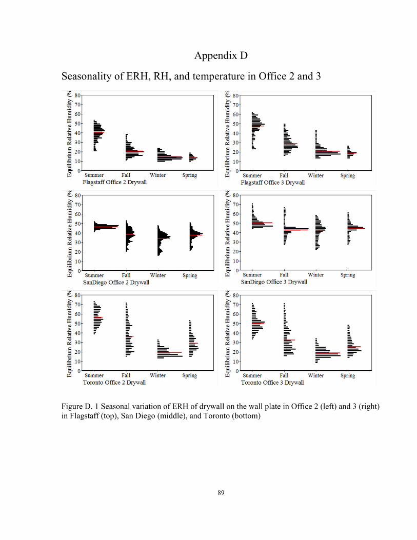
89
Appendix D
Seasonality of ERH, RH, and temperature in Office 2 and 3
Figure D. 1 Seasonal variation of ERH of drywall on the wall plate in Office 2 (left) and 3 (right) in Flagstaff (top), San Diego (middle), and Toronto (bottom)

90
Figure D. 2 Seasonal variation of RH of air on the wall plate in Office 2 (left) and 3 (right) in Flagstaff (top), San Diego (middle), and Toronto (bottom)

91
Figure D. 3 Seasonal variation of air temperature on the wall plate in Office 2 (left) and 3 (right) in Flagstaff (top), San Diego (middle), and Toronto (bottom)

92
Appendix E
Outdoor average temperature
Figure E. 1 Outdoor average high and low temperature from 1974 to 2012 in Flagstaff, San Diego, and Toronto (source: https://weatherspark.com)