The Boson Hubbard model

Subir Sachdev

Department of Physics, Harvard University, Cambridge MA 02138, USA and

School of Natural Sciences, Institute for Advanced Studies, Princeton NJ 08540, USA

(Dated: September 8, 2021)

1

Before turning to the lattice boson Hubbard model, we consider a liquid of bosons in the

continuum, as is appropriate for a description of 4He. In this case, it turns out that the non-

interacting Bose liquid is not a particularly good starting point for understanding the ground state

of bosons with even a weak interaction. Fundamentally new ideas on broken symmetry are needed

to understand the Bose liquid. We first present the theory of the weakly interacting Bose gas, and

will then turn to the lattice model.

I. BOSE GAS IN THE CONTINUUM: BOGOLIUBOV THEORY

We consider bosons bk, where k is a wavevector, interacting with a weak, repulsive short-range

interaction u0. The Bose operator obeys the commutation relation

[bk, b†k′ ] = δk,k′ (1)

and the Hamiltonian is

H =∑k

εkb†kbk +

u02V

∑k,k′,q

b†k+qb†k′−qbk′bk (2)

where V is the volume. In continuum free space the boson dispersion is εk = ~2k2/(2m), where

m is the mass of the boson. But our analysis will also apply for other monotonic dispersions with

a minimum at εk=0 = 0. We assume there is a high momentum cutoff in the interaction term in

(2), beyond which the simple contact form of the interaction does not apply.

We will develop a theory for the ground state of H in a perturbation expansion in u0. At u0 = 0,

the lowest energy state has all bosons in the k = 0 state, with

|G〉 =1√N0

(b†0)N0 |0〉 (3)

where |0〉 is the empty state with no bosons, and N0 is the number of bosons in the k = 0 state.

Once we turn on interactions between the bosons, some fraction of the bosons will occupy non-

zero momenta even in the ground state. Rather than computing this fraction at fixed total particle

number, it turns out to be far easier to describe the ground in the grand canonical ensemble at

a fixed chemical potential µ. In this case, we need to find the state with smallest value for the

‘grand energy’ H − µN , where

N =∑k

b†kbk (4)

To begin, let us just use the state in (3) as a variational trial wavefunction, and evaluate the

expectation value of the grand energy

〈G|H − µN |G〉 = −µN0 +u02V

N0(N0 − 1)

= V[−µn0 +

u02n0(n0 − 1/N)

](5)

2

where

n0 =N0

V(6)

is the density of particles in the k = 0 state. Minimizing (5) with respect to n0 in the thermody-

namic limit (N →∞) we obtain

n0 =µ

u0(7)

and the optimum value of the grand energy is

〈G|H − µN |G〉 = V

[− µ2

2u0

]. (8)

The result in (8) is the leading answer in the small u0 expansion at fixed µ: notice that it diverges

as 1/u0.

We note an important feature of the computation above: the 1/N term in (5) dropped out

in the thermodynamic limit; this term arose from the non-zero commutator [b0, b†0] = 1. The

surviving terms would have been obtained if we had just ignored the non-zero commutator, and

just replaced b0 by the number√N0. This is a consequence of having a non-zero density of particles

at k = 0. Going forward, we will directly use the replacement b0 →√N0, and this will only discard

unimportant terms which vanish in the thermodynamic limit.

We would now like to compute the corrections to (8) at order (u0)0. For this we will need

to include the contributions of the bosons at k 6= 0. We return the original Hamiltonian in (2),

replace b0 →√N0, and keep all terms which are second order in bk, b†k with k 6= 0. This yields

H − µN = V[−µn0 +

u02n20

]+∑k 6=0

(εk − µ+ u0n0) b†kbk

+u0n0

2

∑k 6=0

(b†kb†−k + b−kbk + b†kbk + b†−kb−k

). (9)

The first line of (9) is the same as (5), and we optimized this by choosing n0 in (7). The remaining

lines of (9) describe the Bogoliubov Hamiltonian for bosons with k 6= 0, in which the boson b0 has

been replaced by the number n0 in (7). A notable feature of the Bogoliubov Hamiltonian is that it

appears to not conserve the total number of bosons, with the presence of terms that annihilate or

create pairs of bosons. Of course, the total number of bosons is actually conserved, but by treating

b0 as a number, we are not keeping precise track of the number of bosons in the condensate: in the

thermodynamic limit, we can safely ignore the difference between a condensate with N0 particles

or N0 ± 2 particles.

We can now proceed to diagonalize (9), and so obtain the order (u0)0 correction to the ground

state energy, and also the spectrum of excitation at non-zero k; note that all the terms in the

3

Bogoliubov Hamiltonian are of order (u0)0 after using (7). We can diagonalize (9) by introducing

a new set of bosons, ηk, which obey the canonical Bose commutation relations

[ηk, η†k′ ] = δk,k′ (10)

These are related to the bk by a Bogoliubov transformation

bk = ηk cosh(θk)− η†−k sinh(θk) (11)

with θ−k = θk an arbitrary parameter for now. This transformation has been chosen so that the

commutator (10) implies the commutator (1) and vice versa. Inserting (11) into (9), we find that

we can get all the terms that do not conserve the total number of ηk bosons to cancel provided we

choose

tanh(2θk) =u0n0

εk + u0n0

. (12)

Then the grand Hamiltonian becomes

H − µN = −V µ2

2u0+∑k 6=0

[Ek − εk − u0n0]

+∑k 6=0

Ekη†kηk (13)

where

Ek =√ε2k + 2u0n0εk . (14)

This is the Hamiltonian for free ηk bosons with energy Ek > 0. So the first line of (13) is the

energy of the ground state, which has zero ηk 6=0 bosons i.e. the new ground state is defined by

ηk 6=0 |G〉 = 0. (15)

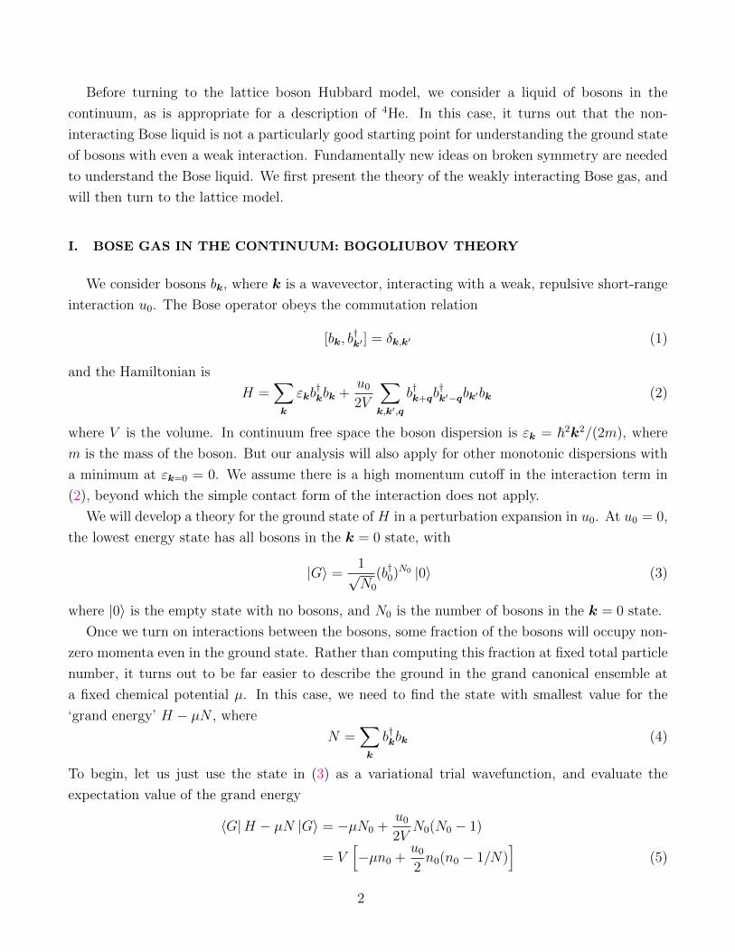
The excited states consist of arbitrary numbers of ηk 6=0 bosons with energy Ek, which is sketched

in Fig. 1. At large |k|, we have the free dispersion of the underlying bosons with Ek ≈ εk. However

at small |k|

Ek → c|k| , c =

√~2u0n0

m(16)

for ε = ~2k2/(2m). So there is a gapless spectrum of linearly-dispersing bosonic particles. It

can be checked that this excitation carries longitudinal density fluctuations (we will see this more

explicitly in Section I B), and so is a ‘phonon’, and c is a sound velocity. The path integral analysis

in Section I B will also show that the gaplessness of the spectrum in (14) is a direct consequence

of a broken symmetry in the ground state of the interacting Bose gas.

The excitation in (16) is sometimes called ‘second sound’ to distinguish it from the usual ‘first

sound’ mode found also in a classical gas. The fundamental distinction between them is that

4

<latexit sha1_base64="46A/fGvrmwI4lz98cQ+hBoLmW7Y=">AAAB6HicbVBNS8NAEJ3Ur1q/qh69LBbBU0mKqMeiF48t2FpoQ9lsJ+3azSbsboQS+gu8eFDEqz/Jm//GbZuDtj4YeLw3w8y8IBFcG9f9dgpr6xubW8Xt0s7u3v5B+fCoreNUMWyxWMSqE1CNgktsGW4EdhKFNAoEPgTj25n/8IRK81jem0mCfkSHkoecUWOl5rhfrrhVdw6ySrycVCBHo1/+6g1ilkYoDRNU667nJsbPqDKcCZyWeqnGhLIxHWLXUkkj1H42P3RKzqwyIGGsbElD5urviYxGWk+iwHZG1Iz0sjcT//O6qQmv/YzLJDUo2WJRmApiYjL7mgy4QmbExBLKFLe3EjaiijJjsynZELzll1dJu1b1Lqu15kWlfpPHUYQTOIVz8OAK6nAHDWgBA4RneIU359F5cd6dj0VrwclnjuEPnM8f1M+M9g==</latexit>

k

<latexit sha1_base64="7BwpfGJvnuAwXX3wkTDBS+khwWU=">AAAB8HicbVDLSgNBEOz1GeMr6tHLYBA8hd0g6jEogscI5iHJEmYns8mQeSwzs0JY8hVePCji1c/x5t84SfagiQUNRVU33V1Rwpmxvv/trayurW9sFraK2zu7e/ulg8OmUakmtEEUV7odYUM5k7RhmeW0nWiKRcRpKxrdTP3WE9WGKflgxwkNBR5IFjOCrZMeb3tZN4rRaNIrlf2KPwNaJkFOypCj3it9dfuKpIJKSzg2phP4iQ0zrC0jnE6K3dTQBJMRHtCOoxILasJsdvAEnTqlj2KlXUmLZurviQwLY8Yicp0C26FZ9Kbif14ntfFVmDGZpJZKMl8UpxxZhabfoz7TlFg+dgQTzdytiAyxxsS6jIouhGDx5WXSrFaCi0r1/rxcu87jKMAxnMAZBHAJNbiDOjSAgIBneIU3T3sv3rv3MW9d8fKZI/gD7/MHZNWQJg==</latexit>

Ek

<latexit sha1_base64="vf7OWqKc3ldpONiiRQjMt2BpiFg=">AAAB6nicdVDLSsNAFL3xWeur6tLNYBFchaQ2bd0V3bisaB/QhjKZTtqhk0mYmQgl9BPcuFDErV/kzr9x+hBU9MCFwzn3cu89QcKZ0o7zYa2srq1vbOa28ts7u3v7hYPDlopTSWiTxDyWnQArypmgTc00p51EUhwFnLaD8dXMb99TqVgs7vQkoX6Eh4KFjGBtpFuCxv1C0bEdr+peVJAhlXLJcwzxPO+85iLXduYowhKNfuG9N4hJGlGhCcdKdV0n0X6GpWaE02m+lyqaYDLGQ9o1VOCIKj+bnzpFp0YZoDCWpoRGc/X7RIYjpSZRYDojrEfqtzcT//K6qQ5rfsZEkmoqyGJRmHKkYzT7Gw2YpETziSGYSGZuRWSEJSbapJM3IXx9iv4nrZLtVuzSTblYv1zGkYNjOIEzcKEKdbiGBjSBwBAe4AmeLW49Wi/W66J1xVrOHMEPWG+fTl2N1Q==</latexit>

ck

<latexit sha1_base64="1fCfowybGua6VefAgxwv3gJovAo=">AAAB/3icdVDLSsNAFJ34rPUVFdy4GSyCq5DEpq27ohuXFewDmrRMppN26OTBzEQoMQt/xY0LRdz6G+78G6cPQUUPXDiccy/33uMnjAppmh/a0vLK6tp6YaO4ubW9s6vv7bdEnHJMmjhmMe/4SBBGI9KUVDLSSThBoc9I2x9fTv32LeGCxtGNnCTEC9EwogHFSCqprx+6AUc4c0c+4j0bjnt2ntlh3tdLpmE6Veu8AhWplG3HVMRxnLOaBS3DnKEEFmj09Xd3EOM0JJHEDAnRtcxEehnikmJG8qKbCpIgPEZD0lU0QiERXja7P4cnShnAIOaqIgln6veJDIVCTEJfdYZIjsRvbyr+5XVTGdS8jEZJKkmE54uClEEZw2kYcEA5wZJNFEGYU3UrxCOkApEqsqIK4etT+D9p2YZVMezrcql+sYijAI7AMTgFFqiCOrgCDdAEGNyBB/AEnrV77VF70V7nrUvaYuYA/ID29gnVJ5YB</latexit>

~2k2

2m

FIG. 1. Excitation spectrum of Bose gas for εk = ~2k2/(2m) with k = |k|.

second sound is a coherent excitation in a collisionless regime, while first sound is a hydrodynamic

mode in a collision dominated regime. Both sound modes exist in the present Bose gas at low T .

We can compute the lifetime of the excitation in Fig. 1 using Fermi’s golden rule from higher order

terms in H that were omitted in the Bogoliubov Hamiltonian: these will lead to a collision time

τk which diverges rapidly as T → 0. Second sound is present in the collisionless regime ωτk � 1,

while first sound is present in the hydrodynamic collision dominated regime ωτk � 1, where we

use |k| = ω/c.

A. Off-diagonal long-range order

A peculiar feature of the ground state we have described above is that the k = 0 wavevector is

treated differently from all non-zero k even in the thermodynamic limit. It would be preferable to

have statement of this feature in terms of correlation functions of local operators, as that would

help generalize the theory to situations where periodic, or even random, potentials are present

and, then the plane wave basis plays no special role. To this end, we introduce the field operator

ψ(r) =1√V

∑k

bkeik·r . (17)

From (1), this obeys the commutation relation

[ψ(r), ψ†(r)] = δ(r − r′) . (18)

We now examine the position-space correlator

⟨ψ†(r)ψ(r′)

⟩=

1

V

∑k

nb(k)eik·(r′−r) (19)

5

where nb(k) is the boson momentum distribution function

nb(k) =⟨b†kbk

⟩, (20)

where we have assumed that⟨b†kbk′

⟩is non-zero only for k = k′). We can evaluate nb(k) by

transforming to the ηk basis using (11), and then at T = 0 we obtain after using (15)

nb(k) =

{N0 k = 0

sinh2(θk) k 6= 0(21)

In the thermodynamic limit (V →∞, N0 →∞, n0 = N0/V fixed), we can write this as

nb(k) = n0(2π)dδ(k) +1

2

(εk + u0n0

Ek

− 1

). (22)

The co-efficient in front of δ(k) can be verified by comparing the integral of (22) with the summation

of (10) over some region of k space including the origin. Finally, we insert (22) into (19) and obtain

⟨ψ†(r)ψ(r′)

⟩= n0 +

∫ddk

(2π)d1

2

(εk + u0n0

Ek

− 1

)eik·(r

′−r) (23)

The important point is that k integral in (23) yields a term which vanishes as |r − r′| → ∞, and

so

lim|r−r′|→∞

⟨ψ†(r)ψ(r′)

⟩= n0 (24)

This is the key statement of off-diagonal long-range order (ODLRO): the left hand side has the

interpretation of an off-diagonal element of the one-particle density matrix, and this does not

vanish as the r and r′ are separated an infinite distance apart. It is a fundamental characteristic

of the ground state of the dilute Bose gas, and indicates the presence of a broken symmetry. As we

raise the temperature, the Bose gas turns into a normal liquid without ODLRO, and the vanishing

of ODLRO implies that this must be accompanied by a phase transition.

It is also useful to contrast the one-particle density matrix of the Bose gas in (23), with that of

the Fermi liquid. In the latter case, the fermion momentum distribution function is characterized

by a discontinuity at the Fermi surface; after a Fourier transform, we obtain for an isotropic Fermi

surface ⟨ψ†(r)ψ(r′)

⟩= Z

∫ kF

0

d3k

(2π)deik·(r

′−r) + . . .

=Z

2π2r3

(sin(kF r)−

cos(kF r)

kF r

)+ . . . (25)

Clearly there is no ODLRO in the Fermi gas. It is replaced by a characteristic term which oscillates

with the Fermi wavevector kF , and has an envelope which decays as 1/r3 in d = 3; the ellipses

indicate terms which decay faster. There are no such oscillatory terms in the Bose gas.

6

B. Path integral theory

The Bogoliubov theory presented above provides a simple intuitive description of the superfluid

ground state. However, some of its features appear mysterious at first glance: e.g. why is the

excitation spectrum gapless, and why does Ek disperse linearly at small k in (16)? Moreover, the

connection of these results to the ODLRO and symmetry breaking is not clear. Many of these

issues are clarified in a path integral theory that we will now describe.

Using the coherent state path integral, we can write the partition function of the boson Hamil-

tonian (2) as the path integral over the boson field ψ(r, τ), where τ is imaginary time extending

on the thermal circle of circumference β = ~/(kBT ), and ψ is periodic around the circle. We have,

setting ~ = kB = 1,

Z = Tre−βH =

∫Dψ(r, τ)e−S (26)

where the action S is

S =

∫ β

0

dτ

∫ddr

[ψ∗∂ψ

∂τ+|∇ψ|2

2m− µ|ψ|2 +

u02|ψ|2

]. (27)

We have specialized to the case where εk = k2/(2m).

We will evaluate path integral by finding the saddle-point of the action, and examining the

fluctuations about the saddle point. The saddle point of (27) is at

ψ =√n0e

iθ0 (28)

where n0 is as in (7), and the angle θ0 is arbitrary. So by picking a saddle point with an arbitrary

value of θ0, we ‘break’ a global U(1) symmetry of the action under which

ψ(r, τ)→ ψ(r, τ)eiθ (29)

where θ is independent of space and time.

Let us now examine fluctuations about the saddle-point (28). It is convenient to parameterize

these fluctuations by 2 real fields, n1(r, τ) and θ(r, τ):

ψ(r, τ) = (n0 + n1(r, τ))1/2 eiθ(r,τ) (30)

It is clear that n1 represents density fluctuations, where θ(r, τ) represents fluctuations in the phase

of the condensate represented by (28). Inserting (30) into (27), we obtain

S = S0 +

∫ β

0

dτ

∫ddr

[in1

∂θ

∂τ+u02n21 +

n0 (∇θ)2

2m+

(∇n1)2

8m(n0 + n1)+ n1

(∇θ)2

2m

](31)

Note that all terms depend only upon the spatial or temporal gradients of θ: this is a consequence

of the global U(1) symmetry (29), and this feature will help us understand the gapless nature of the

7

excitation spectrum. Let us now transform to momentum space, and retain only terms quadratic

in θ and n1 (this will turn out to be equivalent to the Bogoliubov theory). Then (31) yields the

following imaginary time action

S2 =

∫ β

0

dτ∑k

[in1k

∂θ−k∂τ

+1

2

(u0 +

k2

4mn0

)|n1k|2 +

n0k2

2m|θk|2

](32)

This is precisely the action of a set of harmonic oscillators, one for each k, with ‘co-ordinate’ θk,

and canonically conjugate ‘momentum’ n1k. So the density fluctuation of a Bose gas is canonically

conjugate to the phase of the condensate. The energy spectrum of this set of oscillators is most

conveniently obtained by performing the gaussian functional integral over n1k with action S2; this

yields the action for phase fluctuations

Sθ =

∫ β

0

dτ∑k

[1

2(u0 + k2/(4mn0))

∣∣∣∣∂θk∂τ∣∣∣∣2 +

n0k2

2m|θk|2

](33)

This is clearly the action of a set of harmonic oscillators with frequency

ωk =

[n0k

2

m

(u0 +

k2

4mn0

)]1/2(34)

Comparing (34) with (14), we confirm that ωk = Ek, the energy of the ηk bosons in the Bogoliubov

theory: so these bosons are simply the annihilation operators of oscillators representing fluctuations

of the phase of the condensate.

II. BOSONS ON THE LATTICE

Our theory of the Bose gas in Section I was perturbative in the repulsive interaction between

the bosons, u0. This analysis always yields a superfluid ground state for the Bose gas. This chapter

begins our discussion of strong interactions, where the ground state need not be a superfluid, or

for fermions, a Fermi liquid.

For bosons in the continuum, we know from experiments on helium-4 that it realizes a hexagonal-

closed-packed crystalline solid under pressure at T = 0, and this solid has zero helicity modulus.

However, the T = 0 transition from the superfluid to the hcp solid is first order, and no controlled

analytic treatment is available in the vicinity of the transition.

This section will therefore consider a simpler situation: bosons moving on a fixed background

lattice. This situation is realized in ultracold atom systems in the presence of an optical lattice

created by standing waves of lasers. We shall show in this chapter that for lattice bosons, for

a sufficiently strong, but finite, repulsive interaction, there can be quantum transitions from the

superfluid to a gapped non-superfluid phase which is often referred to in this context as an ‘insu-

lator’. We will restrict our attention for now to just on-site repulsive interactions, in which case

8

the Hamiltonian realizes a Hubbard model. Furthermore, the insulating phases we discuss here

do not break the discrete translational symmetry of the background lattice, but such phases do

appear when we include longer-range interactions.

A. Lattice Hamiltonian

We introduce the boson operator bi, which annihilates bosons on the sites, i, of a regular lattice

in d dimensions. These Bose operators and their Hermitian conjugate creation operators obey the

commutation relation [bi, b

†j

]= δij, (35)

while two creation or annihilation operators always commute. It is also useful to introduce the

boson number operator

nbi = b†i bi, (36)

which counts the number of bosons on each site. We allow an arbitrary number of bosons on each

site. Thus the Hilbert space consists of states |{mj}〉, that are eigenstates of the number operators

nbi|{mj}〉 = mi|{mj}〉, (37)

and every mj in the set {mj} is allowed to run over all nonnegative integers. This includes the

“vacuum” state with no bosons at all |{mj = 0}〉.The Hamiltonian of the boson Hubbard model is

HB = −w∑〈ij〉

(b†i bj + b†j bi

)− µ

∑i

nbi + (U/2)∑i

nbi(nbi − 1). (38)

The first term, proportional to w, allows hopping of bosons from site to site (〈ij〉 represents nearest

neighbor pairs); if each site represents a superconducting grain, then w is the Josephson tunneling

that allows Cooper pairs to move between grains. The second term, µ, represents the chemical

potential of the bosons: changing in the value of µ changes the total number of bosons. Depending

upon the physical conditions, a given system can either be constrained to be at a fixed chemical

potential (the grand canonical ensemble) or have a fixed total number of bosons (the canonical

ensemble). Theoretically it is much simpler to consider the fixed chemical potential case, and results

at fixed density can always be obtained from them after a Legendre transformation. Finally, the

last term, U > 0, represents the simplest possible repulsive interaction between the bosons. We

have taken only an on-site repulsion. This can be considered to be the charging energy of each

superconducting grain. Off-site and longer-range repulsion are undoubtedly important in realistic

systems, but these are neglected in this simplest model.

The Hubbard model HB is invariant under a global U(1) ≡ O(2) phase transformation, as in

(29), under which

bi → bieiφ. (39)

9

This symmetry is related to the conservation of the total number of bosons

N b =∑i

nbi; (40)

it is easily verified that N b commutes with H.

We will begin our study of HB by introducing a simple mean-field theory in Section II B. This

mean field theory displays superfluid-insulator transitions, and we will employ the coherent state

path integral approach to obtain continuum quantum theories describing fluctuations near the

quantum critical points in Section II C. Our treatment builds on the work of Fisher et al. [1].

B. Mean field theory

The strategy, as in any mean-field theory, will be to model the properties of HB by the best

possible sum, HMF, of single-site Hamiltonians:

HMF =∑i

(−µnbi + (U/2) nbi(nbi − 1)−Ψ∗B bi −ΨB b

†i

), (41)

where the complex number ΨB is a variational parameter. We have chosen a mean-field Hamilto-

nian with the same on-site terms as HB and have added an additional term with a “field” ΨB to

represent the influence of the neighboring sites; this field has to be self-consistently determined.

Notice that this term breaks the U(1) symmetry and does not conserve the total number of par-

ticles. This is to allow for the possibility of broken-symmetric phases, whereas symmetric phases

will appear at the special value ΨB = 0. As we saw in the analysis of HR, the state that breaks

the U(1) symmetry will have a nonzero stiffness to rotations of the order parameter; in the present

case this stiffness is the superfluid density characterizing a superfluid ground state of the bosons.

Another important assumption underlying (41) is that the ground state does not spontaneously

break a translational symmetry of the lattice, as the mean-field Hamiltonian is the same on ev-

ery site. Such a symmetry breaking is certainly a reasonable possibility, but we will ignore this

complication here for simplicity.

We will determine the optimum value of the mean-field parameter ΨB by a standard procedure.

First, determine the ground state wavefunction of HMF for an arbitrary ΨB; because HMF is a sum

of single-site Hamiltonians, this wavefunction will simply be a product of single-site wavefunctions.

Next, evaluate the expectation value of HB in this wavefunction. By adding and subtracting HMF

from HB, we can write the mean-field value of the ground state energy of HB in the form

E0

M=EMF(ΨB)

M− Zw

⟨b†⟩〈b〉+ 〈b〉Ψ∗B +

⟨b†⟩ΨB, (42)

where EMF(ΨB) is the ground state energy of HMF, M is the number of sites of the lattice, Z is

the number of nearest neighbors around each lattice point (the “coordination number”), and the

10

-1

0

1

2

3

0 0.1 0.2 0.3

Superfluid

M.I. 3

M.I. 2

M.I. 0

M.I. 1

µ /U

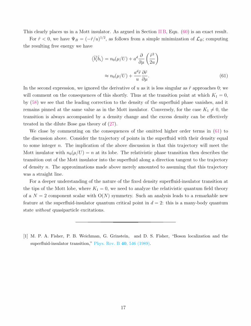
Zw/U

FIG. 2. Mean-field phase diagram of the ground state of the boson Hubbard model HB in (38). The

notation M.I. n refers to a Mott insulator with n0(µ/U) = n.

expectation values are evaluated in the ground state of HMF. The final step is to minimize (42)

over variations in ΨB. We have carried out this step numerically and the results are shown in

Fig. 2.

Notice that even on a single site, HMF has an infinite number of states, corresponding to the

allowed values m ≥ 0 of the integer number of bosons on each site. The numerical procedure

necessarily truncates these states at some large occupation number, but the errors are not difficult

to control. In any case, we will show that all the essential properties of the phase diagram can be

obtained analytically. Also, by taking the derivative of (42) with respect to ΨB, it is easy to show

that at the optimum value of ΨB

ΨB = Zw〈b〉; (43)

this relation, however, does not hold at a general point in parameter space.

First, let us consider the limit w= 0. In this case the sites are decoupled, and the mean-

field theory is exact. It is also evident that ΨB = 0, and we simply have to minimize the on-site

interaction energy. The on-site Hamiltonian contains only the operator n, and the solution involves

finding the boson occupation number (which are the integer-valued eigenvalues of n) that minimizes

HB. This is simple to carry out, and we get the ground state wavefunction

|mi = n0(µ/U)〉 , (44)

11

where the integer-valued function n0(µ/U) is given by

n0(µ/U) =

0, for µ/U < 0,

1, for 0 < µ/U < 1,

2, for 1 < µ/U < 2,...

...

n, for n− 1 < µ/U < n.

(45)

Thus each site has exactly the same integer number of bosons, which jumps discontinuously when-

ever µ/U goes through a positive integer. When µ/U is exactly equal to a positive integer, there

are two degenerate states on each site (with boson numbers differing by 1) and so the entire system

has a degeneracy of 2M . This large degeneracy implies a macroscopic entropy; it will be lifted once

we turn on a nonzero w.

We now consider the effects of a small nonzero w. As is shown in Fig. 2, the regions with

ΨB = 0 survive in lobes around each w = 0 state (44) characterized by a given integer value of

n0(µ/U). Only at the degenerate point with µ/U = integer does a nonzero w immediately lead to

a state with ΨB 6= 0. We will consider the properties of this ΨB 6= 0 later, but now we discuss the

properties of the lobes with ΨB = 0 in some more detail. In mean-field theory, these states have

wavefunctions still given exactly by (44). However, it is possible to go beyond mean-field theory

and make an important exact statement about each of the lobes: The expectation value of the

number of bosons in each site is given by⟨b†i bi⟩

= n0(µ/U), (46)

which is the same result one would obtain from the product state (44) (which, we emphasize, is

not the exact wavefunction for w 6= 0). There are two important ingredients behind the result

(46): the existence of an energy gap and the fact that N b commutes with HB. First, recall that at

w = 0, provided µ/U was not exactly equal to a positive integer, there was a unique ground state,

and there was a nonzero energy separating this state from all other states (this is the energy gap).

As a result, when we turn on a small nonzero w, the ground state will move adiabatically without

undergoing any level crossings with any other state. Now the w = 0 state is an exact eigenstate of

N b with eigenvalue Mn0(µ/U), and the perturbation arising from a nonzero w commutes with N b.

Consequently, the ground state will remain an eigenstate of N b with precisely the same eigenvalue,

Mn0(µ/U), even for small nonzero w. Assuming translational invariance, we then immediately

have the exact result (46). Notice that this argument also shows that the energy gap above the

ground state will survive everywhere within the lobe. These regions with a quantized value of the

density and an energy gap to all excitations are known as “Mott insulators.” Their ground states

are very similar to, but not exactly equal to, the simple state (44): They involve in addition terms

with bosons undergoing virtual fluctuations between pairs of sites, creating particle–hole pairs.

12

The Mott insulators are also known as “incompressible” because their density does not change

under changes of the chemical potential µ or other parameters in HB:

∂〈N b〉∂µ

= 0. (47)

It is worth reemphasizing here the remarkable nature of the exact result (46). From the per-

spective of classical critical phenomena, it is most unusual to find the expectation value of any

observable to be pinned at a quantized value over a finite region of the phase diagram. The exis-

tence of observables such as N b that commute with the Hamiltonian is clearly a crucial ingredient.

The numerical analysis shows that the boundary of the Mott insulating phases is a second-

order quantum phase transition (i.e., a nonzero ΨB turns on continuously). With the benefit of

this knowledge, we can determine the positions of the phase boundaries. By the usual Landau

theory argument, we simply need to expand E0 in (42) in powers of ΨB,

E0 = E00 + r|ΨB|2 +O(|ΨB|4), (48)

and the phase boundary appears when r changes sign. The value of r can be computed from (42)

and (41) by second-order perturbation theory, and we find

r = χ0(µ/U) [1− Zwχ0(µ/U)] , (49)

where

χ0(µ/U) =n0(µ/U) + 1

Un0(µ/U)− µ+

n0(µ/U)

µ− U(n0(µ/U)− 1). (50)

The function n0(µ/U) in (45) is such that the denominators in (50) are positive, except at the

points at which boson occupation number jumps at w = 0. The solution of the simple equation

r = 0 leads to the phase boundaries shown in Fig. 2.

Finally, we turn to the phase with ΨB 6= 0. The mean-field parameter ΨB varies continuously

as the parameters are varied. As a result all thermodynamic variables also change, and the density

does not take a quantized value; by a suitable choice of parameters, the average density can be

varied smoothly across any real positive value. So this is a compressible state in which

∂〈N b〉∂µ

6= 0. (51)

As we noted earlier, the presence of a ΨB 6= 0 implies that the U(1) symmetry is broken, and there

is a nonzero stiffness (i.e. helicity modulus) to twists in the orientation of the order parameter.

We also note that extensions of the boson Hubbard model with interactions beyond nearest

neighbor can spontaneously break translational symmetry at certain densities. If this symmetry

breaking coexists with the superfluid order, one can obtain a “supersolid” phase.

13

C. Continuum quantum field theories

Returning to our discussion of the boson Hubbard model, here we will describe the low-energy

properties of the quantum phase transitions between the Mott insulators and the superfluid found

in Section II B. We will find that it is crucial to distinguish between two different cases, each

characterized by its own universality class and continuum quantum field theory. The important

diagnostic distinguishing the two possibilities will be the behavior of the boson density across the

transition. In the Mott insulator, this density is of course always pinned at some integer value. As

one undergoes the transition to the superfluid, depending upon the precise location of the system

in the phase diagram of Fig. 2, there are two possible behaviors of the density: (A) The density

remains pinned at its quantized value in the superfluid in the vicinity of the quantum critical point,

or (B) the transition is accompanied by a change in the density.

We begin by writing the partition function of HB, ZB = Tre−HB/T in the coherent state path

integral representation:

ZB =

∫Dbi(τ)Db†i (τ) exp

(−∫ 1/T

0

dτLb

),

Lb =∑i

(b†idbidτ− µb†ibi + (U/2) b†ib

†ibibi

)− w

∑〈ij〉

(b†ibj + b†jbi

).

(52)

Here we have changed notation ψ(τ) → b(τ), as is conventional; we are dealing exclusively with

path integrals from now on, and so there is no possibility of confusion with the operators b in the

Hamiltonian language. Also note that the repulsion proportional to U in (38) becomes the product

of four boson operators above after normal ordering.

It is clear that the critical field theory of the superfluid-insulator transition should be expressed

in terms of a spacetime-dependent field ΨB(x, τ), which is analogous to the mean-field parame-

ter ΨB appearing in Section II B. Such a field is most conveniently introduced by the applying

the Hubbard–Stratanovich transformation on the coherent state path integral. We decouple the

hopping term proportional to w by introducing an auxiliary field ΨBi(τ) and transforming ZB to

ZB =

∫Dbi(τ)Db†i (τ)DΨBi(τ)DΨ†Bi(τ) exp

(−∫ 1/T

0

dτL′b

),

L′b =∑i

(b†idbidτ− µb†ibi + (U/2) b†ib

†ibibi −ΨBib

†i −Ψ∗Bibi

)+∑i,j

Ψ∗Biw−1ij ΨBj. (53)

We have introduced the symmetric matrix wij whose elements equal w if i and j are nearest neigh-

bors and vanish otherwise. The equivalence between (53) and (52) can be easily established, by

14

simply carrying out the Gaussian integral over ΨB; this also generates some overall normalization

factors, but these have been absorbed into a definition of the measure DΨB. Let us also note a

subtlety we have glossed over: Strictly speaking, the transformation between (53) and (52) requires

that all the eigenvalues of wij be positive, for only then are the Gaussian integrals over ΨB well

defined. This is not the case for, say, the hypercubic lattice, which has negative eigenvalues for

wij. This can be repaired by adding a positive constant to all the diagonal elements of wij and

subtracting the same constant from the on-site b part of the Hamiltonian. We will not explicitly do

this here as our interest is only in the long-wavelength modes of the ΨB field, and the corresponding

eigenvalues of wij are positive.

For our future purposes, it is useful to describe an important symmetry property of (53).

Notice that the functional integrand is invariant under the following time-dependent U(1) gauge

transformation:

bi → bieiφ(τ),

ΨBi → ΨBieiφ(τ), (54)

µ→ µ+ i∂φ

∂τ.

The chemical potential µ becomes time dependent above, and so this transformation takes one out

of the physical parameter regime; nevertheless (54) is very useful, as it places important restrictions

on subsequent manipulations of ZB.

The next step is to integrate out the bi, b†i fields from (53). This can be done exactly in powers

of ΨB and Ψ∗B: The coefficients are simply products of Green’s functions of the bi. The latter can

be determined in closed form because the ΨB-independent part of L′b is simply a sum of single-

site Hamiltonians for the bi: these were exactly diagonalized in (44), and all single-site Green’s

functions can also be easily determined. We re-exponentiate the resulting series in powers of ΨB,

Ψ∗B and expand the terms in spatial and temporal gradients of ΨB. The expression for ZB can

now be written as [1]

ZB =

∫DΨB(x, τ)DΨ∗B(x, τ) exp

(−V F0

T−∫ 1/T

0

dτ

∫ddxLB

), (55)

LB = K1Ψ∗B

∂ΨB

∂τ+K2

∣∣∣∣∂ΨB

∂τ

∣∣∣∣2 +K3 |∇ΨB|2 + r|ΨB|2 +u

2|ΨB|4 + · · · .

Here V = Mad is the total volume of the lattice, and ad is the volume per site. The quantity F0 is

the free energy density of a system of decoupled sites; its derivative with respect to the chemical

potential gives the density of the Mott insulating state, and so

− ∂F0

∂µ=n0(µ/U)

ad. (56)

15

The other parameters in (55) can also be expressed in terms of µ, U , and w but we will not display

explicit expressions for all of them. Most important is the parameter r, which can be seen to be

rad =1

Zw− χ0(µ/U), (57)

where χ0 was defined in (50). Notice that r is proportional to the mean-field r in (49); in particular,

r vanishes when r vanishes, and the two quantities have the same sign. The mean-field critical

point between the Mott insulator and the superfluid appeared at r = 0, and it is not surprising

that the mean-field critical point of the continuum theory (55) is given by the same condition.

Of the other couplings in (55), K1, the coefficient of the first-order time derivative also plays a

crucial role. It can be computed explicitly, but it is simpler to note that the value of K1 can be

fixed by demanding that (55) be invariant under (54) for small φ: A simple calculation shows that

we must have

K1 = −∂ r∂µ

. (58)

This relationship has a very interesting consequence. Notice that K1 vanishes when r is µ-

independent; however, this is precisely the condition that the Mott insulator–superfluid phase

boundary in Fig. 2 have a vertical tangent (i.e., at the tips of the Mott insulating lobes). This is

significant because at the value K1 = 0 (55) is a relativistic field theory for a complex scalar field

ΨB. So the Mott insulator to superfluid transition is in the universality class of a relativistic scalar

field theory for K1 = 0.

In contrast, for K1 6= 0 we have a rather different field theory with a first-order time derivative:

in this case we can drop the K2 term as it involves two time derivatives and so is irrelevant with

respect to the single time derivative in the K1 term; then the field theory in (55) is identical to the

theory (27) for the dilute Bose case in Section I. However, in the present situation, the bosons are

not necessarily dilute; instead, we have shown that the excess density of bosons over the density

of the Mott insulator can be effectively treated as a dilute gas.

To conclude this discussion, we would like to correlate the above discussion on the distinction

between the two universality classes with the behavior of the boson density across the transition.

This can be evaluated by taking the derivative of the total free energy with respect to the chemical

potential, as is clear from (38): ⟨b†i bi⟩

= −ad∂F0

∂µ− ad∂FB

∂µ

= n0(µ/U)− ad∂FB∂µ

, (59)

where FB is the free energy resulting from the functional integral over ΨB in (55).

In mean-field theory, for r > 0, we have ΨB = 0, and therefore FB = 0, implying⟨b†i bi⟩

= n0(µ/U), for r > 0. (60)

16

This clearly places us in a Mott insulator. As argued in Section II B, Eqn. (60) is an exact result.

For r < 0, we have ΨB = (−r/u)1/2, as follows from a simple minimization of LB; computing

the resulting free energy we have⟨b†i bi⟩

= n0(µ/U) + ad∂

∂µ

(r2

2u

)

≈ n0(µ/U) +adr

u

∂r

∂µ. (61)

In the second expression, we ignored the derivative of u as it is less singular as r approaches 0; we

will comment on the consequences of this shortly. Thus at the transition point at which K1 = 0,

by (58) we see that the leading correction to the density of the superfluid phase vanishes, and it

remains pinned at the same value as in the Mott insulator. Conversely, for the case K1 6= 0, the

transition is always accompanied by a density change and the excess density can be effectively

treated in the dilute Bose gas theory of (27).

We close by commenting on the consequences of the omitted higher order terms in (61) to

the discussion above. Consider the trajectory of points in the superfluid with their density equal

to some integer n. The implication of the above discussion is that this trajectory will meet the

Mott insulator with n0(µ/U) = n at its lobe. The relativistic phase transition then describes the

transition out of the Mott insulator into the superfluid along a direction tangent to the trajectory

of density n. The approximations made above merely amounted to assuming that this trajectory

was a straight line.

For a deeper understanding of the nature of the fixed density superfluid-insulator transition at

the tips of the Mott lobe, where K1 = 0, we need to analyze the relativistic quantum field theory

of a N = 2 component scalar with O(N) symmetry. Such an analysis leads to a remarkable new

feature at the superfluid-insulator quantum critical point in d = 2: this is a many-body quantum

state without quasiparticle excitations.

[1] M. P. A. Fisher, P. B. Weichman, G. Grinstein, and D. S. Fisher, “Boson localization and the

superfluid-insulator transition,” Phys. Rev. B 40, 546 (1989).

17