The Bayes Net Toolbox for Matlaband applications to computer vision

Kevin MurphyMIT AI lab

Outline of talk

• BNT

Outline of talk

• BNT

• Using graphical models for visual object detection

Outline of talk

• BNT

• Using graphical models (but not BNT!) for visual object detection

• Lessons learned: my new software philosophy

Outline of talk: BNT

• What is BNT?

• How does BNT compare to other GM packages?

• How does one use BNT?

What is BNT?• BNT is an open-source collection of matlab

functions for (directed) graphical models:– exact and approximate inference

– parameter and structure learning

• Over 100,000 hits and about 30,000 downloads since May 2000

• Ranked #1 by Google for “Bayes Net software”• About 43,000 lines of code (of which 8,000 are

comments) • Typical users: students, teachers, biologists

www.ai.mit.edu/~murphyk/Software/BNT/bnt.html

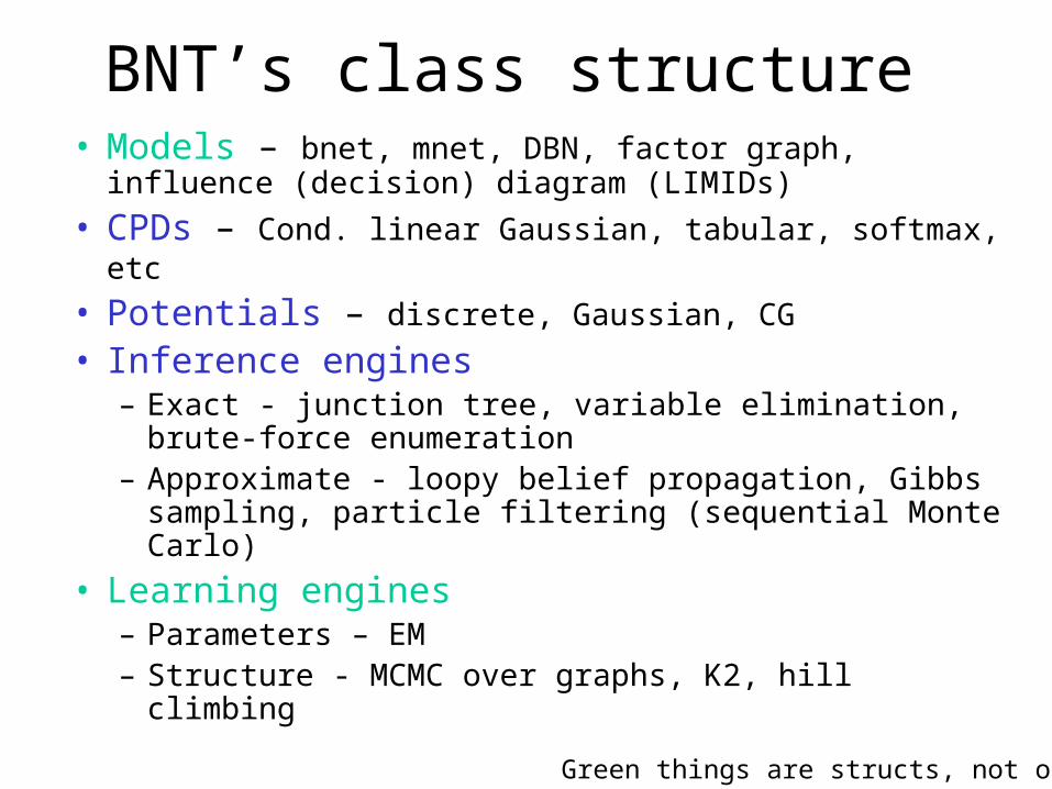
BNT’s class structure• Models – bnet, mnet, DBN, factor graph, influence (decision)

diagram (LIMIDs)

• CPDs – Cond. linear Gaussian, tabular, softmax, etc • Potentials – discrete, Gaussian, CG

• Inference engines– Exact - junction tree, variable elimination, brute-force

enumeration– Approximate - loopy belief propagation, Gibbs sampling,

particle filtering (sequential Monte Carlo)

• Learning engines– Parameters – EM– Structure - MCMC over graphs, K2, hill climbing

Green things are structs, not objects

Kinds of models that BNT supports• Classification/ regression: linear regression, logistic regression,

cluster weighted regression, hierarchical mixtures of experts, naïve Bayes

• Dimensionality reduction: probabilistic PCA, factor analysis, probabilistic ICA

• Density estimation: mixtures of Gaussians• State-space models: LDS, switching LDS, tree-structured AR models• HMM variants: input-output HMM, factorial HMM, coupled HMM,

DBNs• Probabilistic expert systems: QMR, Alarm, etc.• Limited-memory influence diagrams (LIMID)• Undirected graphical models (MRFs)

Brief history of BNT

• Summer 1997: started C++ prototype while intern at DEC/Compaq/HP CRL

• Summer 1998: First public release (while PhD student at UC Berkeley)

• Summer 2001: Intel decided to adopt BNT as prototype for PNL

Why Matlab?• Pros (similar to R)

– Excellent interactive development environment– Excellent numerical algorithms (e.g., SVD)– Excellent data visualization– Many other toolboxes, e.g., netlab, image processing– Code is high-level and easy to read (e.g., Kalman filter in 5 lines of code)– Matlab is the lingua franca of engineers and NIPS

• Cons:– Slow– Commercial license is expensive– Poor support for complex data structures

• Other languages I would consider in hindsight:– R, Lush, Ocaml, Numpy, Lisp, Java

Why yet another BN toolbox?• In 1997, there were very few BN programs, and all failed to satisfy the

following desiderata:– Must support vector-valued data (not just discrete/scalar)– Must support learning (parameters and structure)– Must support time series (not just iid data)– Must support exact and approximate inference– Must separate API from UI– Must support MRFs as well as BNs– Must be possible to add new models and algorithms– Preferably free– Preferably open-source– Preferably easy to read/ modify – Preferably fast

BNT meets all these criteria except for the last

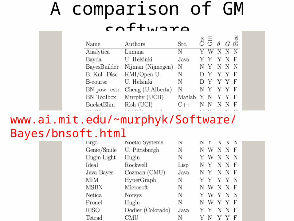
A comparison of GM software

www.ai.mit.edu/~murphyk/Software/Bayes/bnsoft.html

Summary of existing GM software• ~8 commercial products (Analytica, BayesiaLab,

Bayesware, Business Navigator, Ergo, Hugin, MIM,

Netica); most have free “student” versions

• ~30 academic programs, of which ~20 have source code (mostly Java, some C++/ Lisp)

• See appendix of book by Korb & Nicholson (2003)

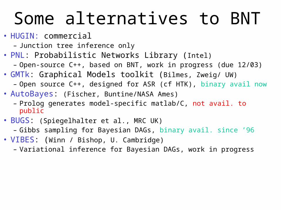
Some alternatives to BNT• HUGIN: commercial

– Junction tree inference only

• PNL: Probabilistic Networks Library (Intel)– Open-source C++, based on BNT, work in progress (due 12/03)

• GMTk: Graphical Models toolkit (Bilmes, Zweig/ UW)– Open source C++, designed for ASR (cf HTK), binary avail now

• AutoBayes: (Fischer, Buntine/NASA Ames)– Prolog generates model-specific matlab/C, not avail. to public

• BUGS: (Spiegelhalter et al., MRC UK)– Gibbs sampling for Bayesian DAGs, binary avail. since ’96

• VIBES: (Winn / Bishop, U. Cambridge)– Variational inference for Bayesian DAGs, work in progress

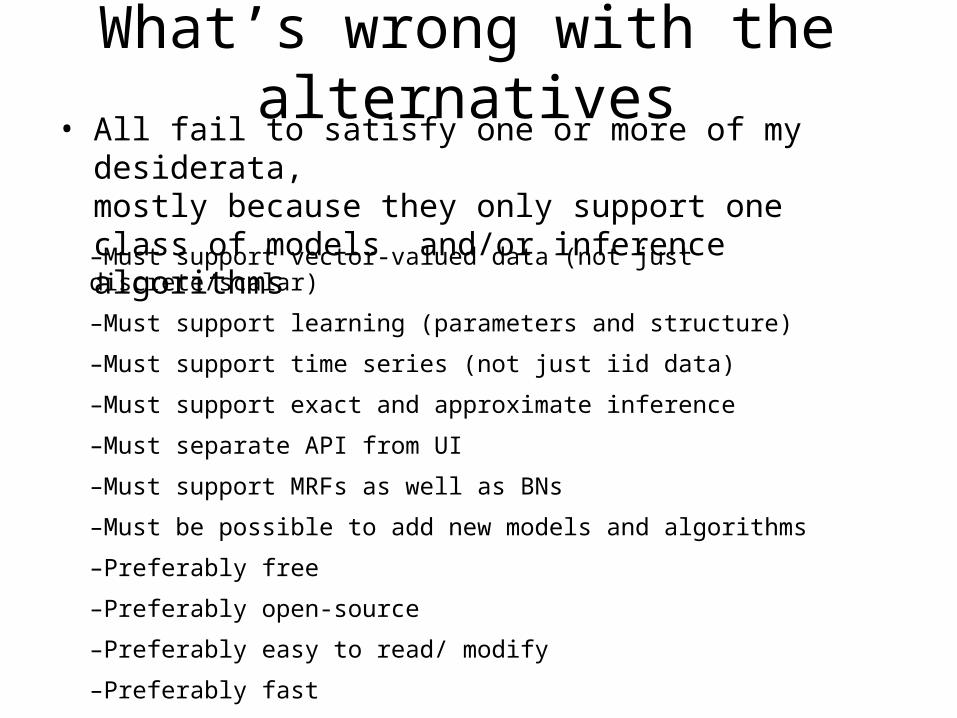
What’s wrong with the alternatives• All fail to satisfy one or more of my desiderata,

mostly because they only support one class of models and/or inference algorithms

–Must support vector-valued data (not just discrete/scalar)

–Must support learning (parameters and structure)

–Must support time series (not just iid data)

–Must support exact and approximate inference

–Must separate API from UI

–Must support MRFs as well as BNs

–Must be possible to add new models and algorithms

–Preferably free

–Preferably open-source

–Preferably easy to read/ modify

–Preferably fast

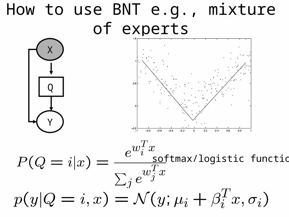
How to use BNT e.g., mixture of experts

X

Y

Q

softmax/logistic function

1. Making the graph

X

Y

Q

X = 1; Q = 2; Y = 3;dag = zeros(3,3);dag(X, [Q Y]) = 1;dag(Q, Y) = 1;

•Graphs are (sparse) adjacency matrices•GUI would be useful for creating complex graphs•Repetitive graph structure (e.g., chains, grids) is bestcreated using a script (as above)

2. Making the model

node_sizes = [1 2 1];dnodes = [2];bnet = mk_bnet(dag, node_sizes, … ‘discrete’, dnodes);

X

Y

Q

•X is always observed input, hence only one effective value•Q is a hidden binary node•Y is a hidden scalar node•bnet is a struct, but should be an object•mk_bnet has many optional arguments, passed as string/value pairs

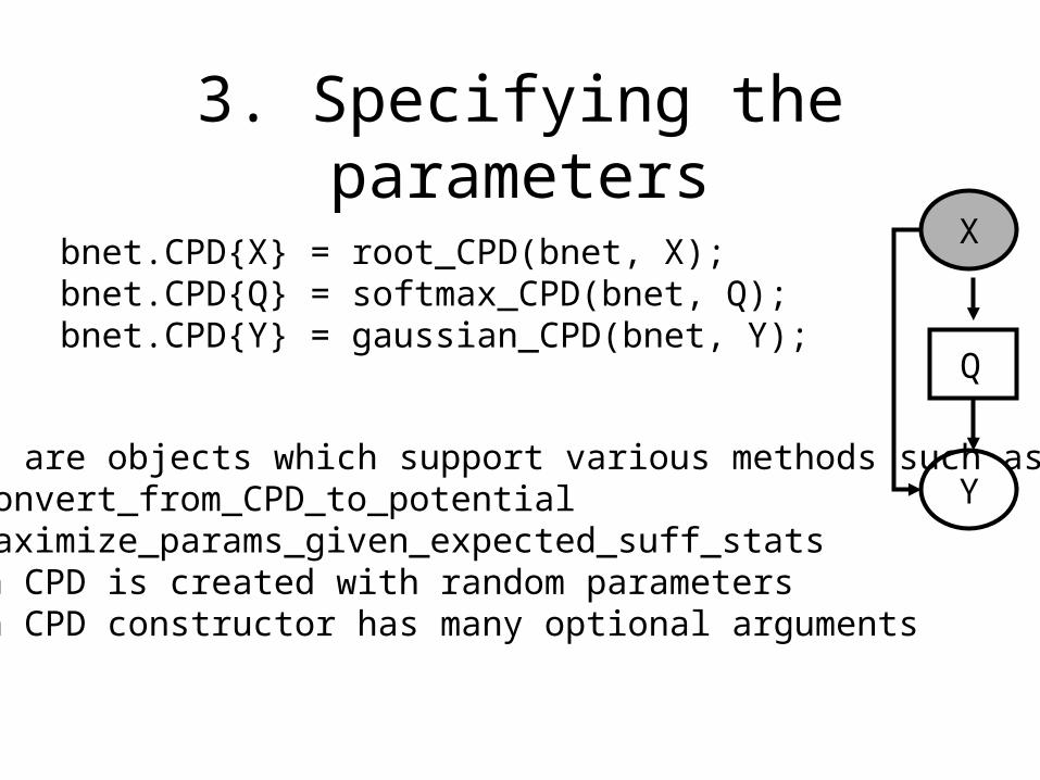
3. Specifying the parametersX

Y

Q

bnet.CPD{X} = root_CPD(bnet, X);bnet.CPD{Q} = softmax_CPD(bnet, Q);bnet.CPD{Y} = gaussian_CPD(bnet, Y);

•CPDs are objects which support various methods such as•Convert_from_CPD_to_potential•Maximize_params_given_expected_suff_stats

•Each CPD is created with random parameters•Each CPD constructor has many optional arguments

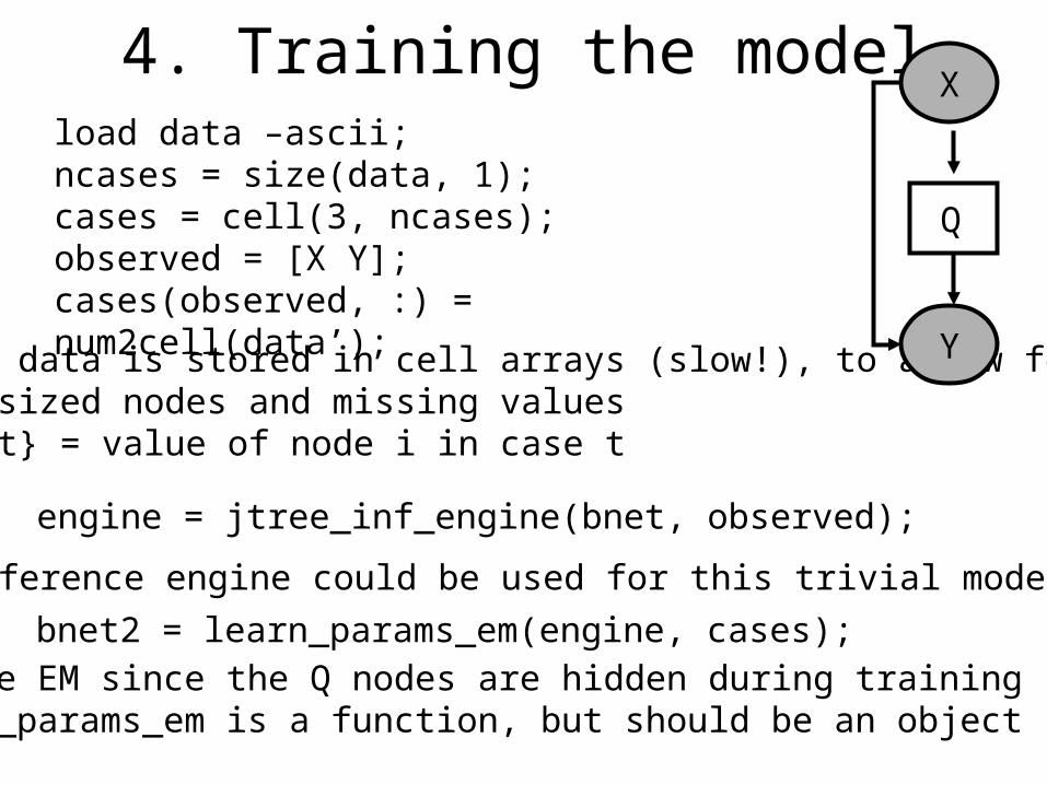
4. Training the modelload data –ascii;ncases = size(data, 1);cases = cell(3, ncases);observed = [X Y];cases(observed, :) = num2cell(data’);•Training data is stored in cell arrays (slow!), to allow for

variable-sized nodes and missing values•cases{i,t} = value of node i in case t

engine = jtree_inf_engine(bnet, observed);

•Any inference engine could be used for this trivial model

bnet2 = learn_params_em(engine, cases);•We use EM since the Q nodes are hidden during training•learn_params_em is a function, but should be an object

X

Y

Q

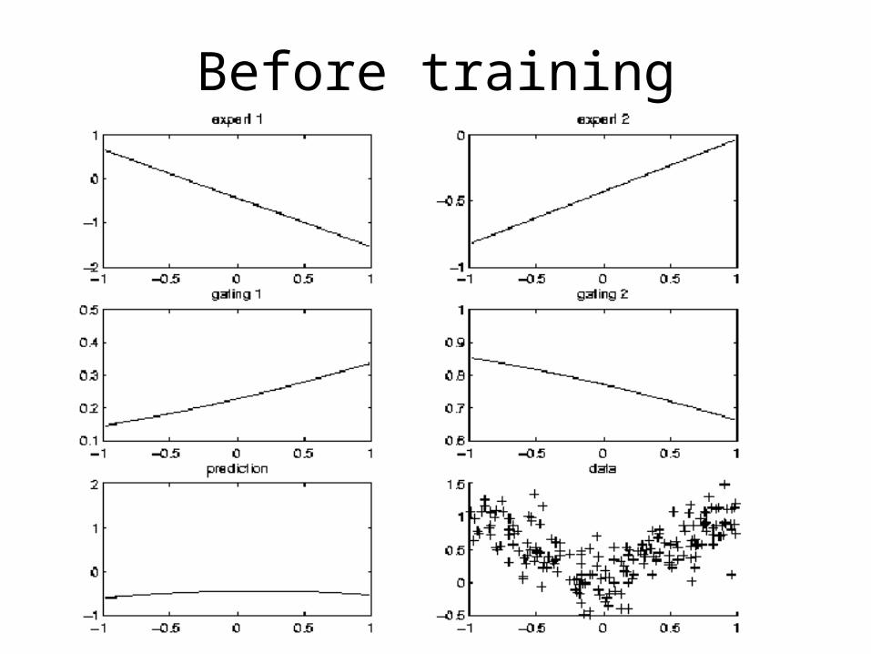
Before training

After training

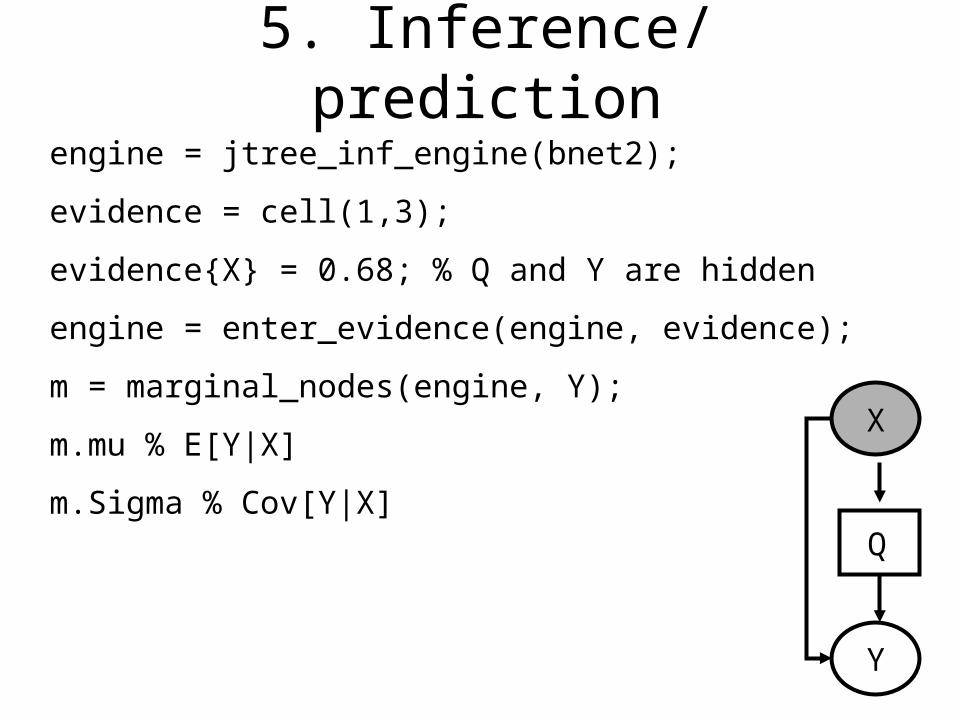
5. Inference/ prediction

engine = jtree_inf_engine(bnet2);

evidence = cell(1,3);

evidence{X} = 0.68; % Q and Y are hidden

engine = enter_evidence(engine, evidence);

m = marginal_nodes(engine, Y);

m.mu % E[Y|X]

m.Sigma % Cov[Y|X]

X

Y

Q

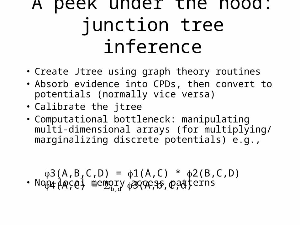
A peek under the hood:junction tree inference

• Create Jtree using graph theory routines• Absorb evidence into CPDs, then convert to

potentials (normally vice versa)• Calibrate the jtree• Computational bottleneck: manipulating multi-

dimensional arrays (for multiplying/ marginalizing discrete potentials) e.g.,

• Non-local memory access patterns

3(A,B,C,D) = 1(A,C) * 2(B,C,D)4(A,C) = b,d 3(A,b,C,d)

Summary of BNT

• CPDs are like “lego bricks”

• Provides many inference algorithms, with different speed/ accuracy/ generality tradeoffs (to be chosen by user)

• Provides several learning algorithms (parameters and structure)

• Source code is easy to read and extend

What’s wrong with BNT?• It is slow

• It has little support for undirected models

• It does not support online inference/learning

• It does not support Bayesian estimation• It has no GUI

• It has no file parser

• It relies on Matlab, which is expensive

• It is too difficult to integrate with real-world applications e.g., visual object detection

Outline of talk: object detection

• What is object detection?• Standard approach to object detection• Some problems with the standard approach• Our proposed solution: combine local,

bottom-up information with global, top-down information using a graphical model

What is object detection?

Goal: recognize 10s of objects in real-time from wearable camera

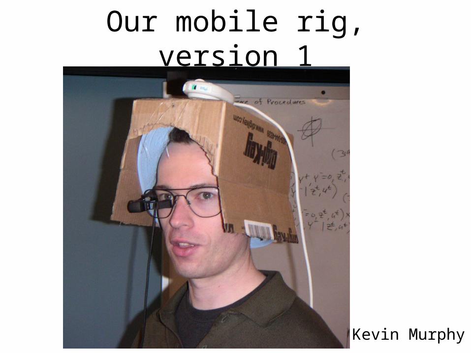
Our mobile rig, version 1

Kevin Murphy

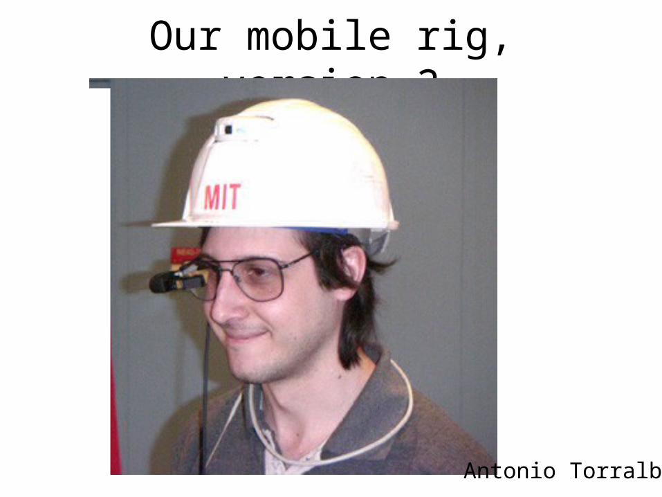
Our mobile rig, version 2

Antonio Torralba

Classify local image patches at each location and scale.

Standard approach to object detection

Localfeatures no car

Classifierp( car | VL )

VL

Popular classifiers use SVMs or boosting.Popular features are raw pixel intensity or wavelet outputs.

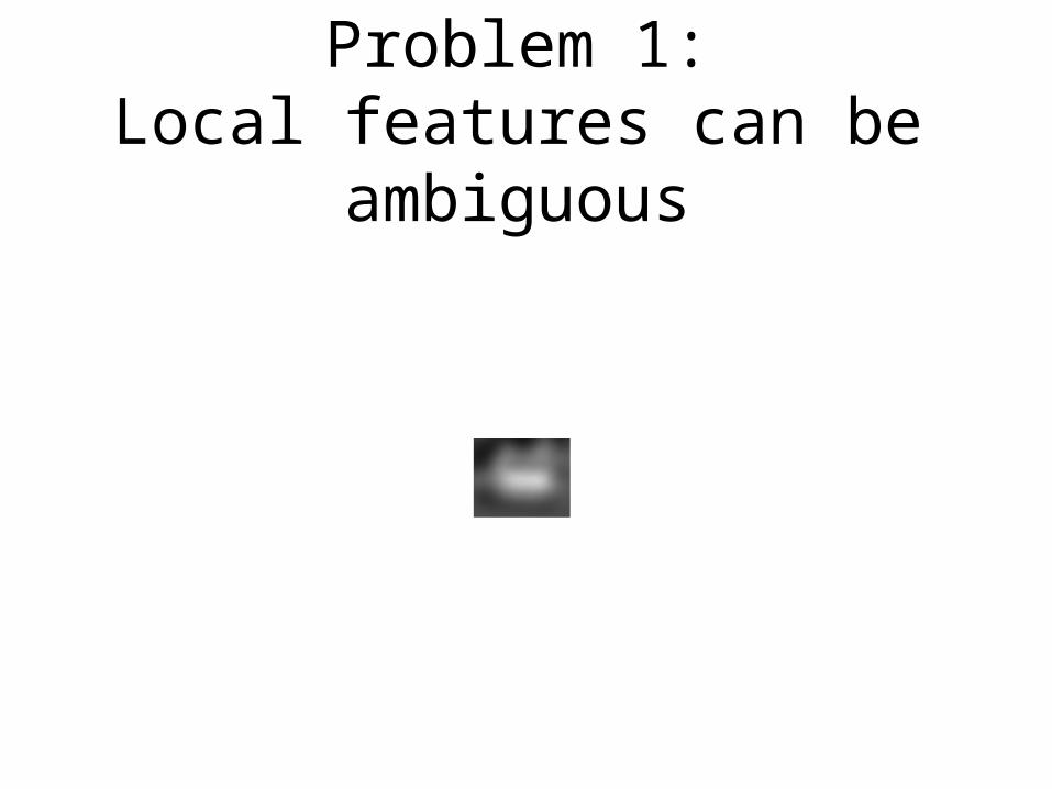
Problem 1:Local features can be ambiguous

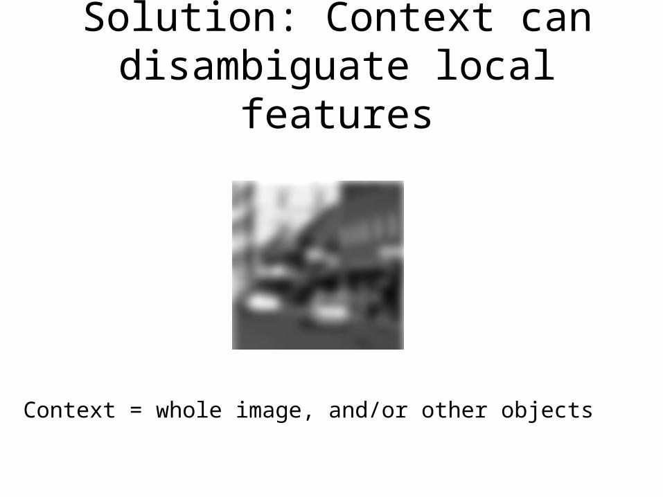
Solution: Context can disambiguate local features

Context = whole image, and/or other objects

carpedestrian

Effect of context on object detection

ash tray

Images by A. Torralba

carpedestrian

Identical local image features!

Effect of context on object detection

ash tray

Images by A. Torralba

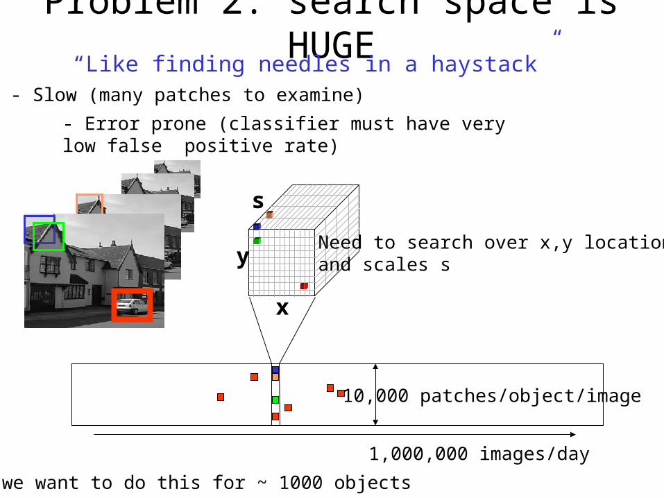
Problem 2: search space is HUGE

x

1,000,000 images/day

Plus, we want to do this for ~ 1000 objects

y

s

- Error prone (classifier must have very low false positive rate)

“Like finding needles in a haystack”- Slow (many patches to examine)

10,000 patches/object/image

Need to search over x,y locationsand scales s

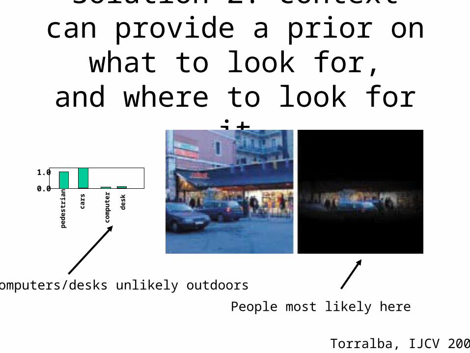
Solution 2: context can provide a prior on what to look for,and where to look for it

People most likely here

Torralba, IJCV 2003

cars

1.0

0.0

ped e

stri

a n

com

put e

r

desk

Computers/desks unlikely outdoors

Outline of talk: object detection

• What is object detection?• Standard approach to object detection• Some problems with the standard approach• Our proposed solution: combine local,

bottom-up information with global, top-down information using a graphical model

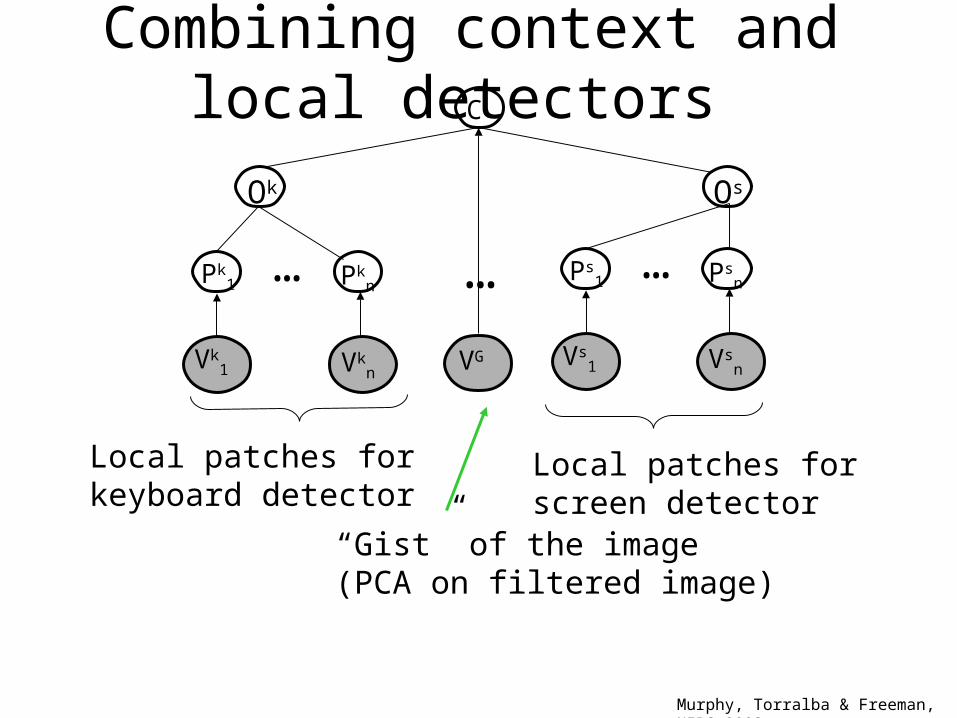
Combining context and local detectors

Murphy, Torralba & Freeman, NIPS 2003

Vkn

Pk1

Ok

Pkn

Vk1

…

C

Vsn

Ps1

Os

Psn

Vs1

…

VG

…

“Gist” of the image(PCA on filtered image)

Local patches forkeyboard detector

Local patches forscreen detector

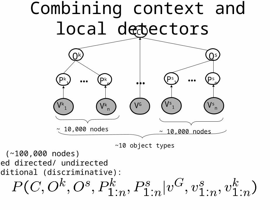
Combining context and local detectors

1. Big (~100,000 nodes)2. Mixed directed/ undirected3. Conditional (discriminative):

Vkn

Pk1

Ok

Pkn

Vk1

…

C

Vsn

Ps1

Os

Psn

Vs1

…

VG

~ 10,000 nodes~ 10,000 nodes

~10 object types

…

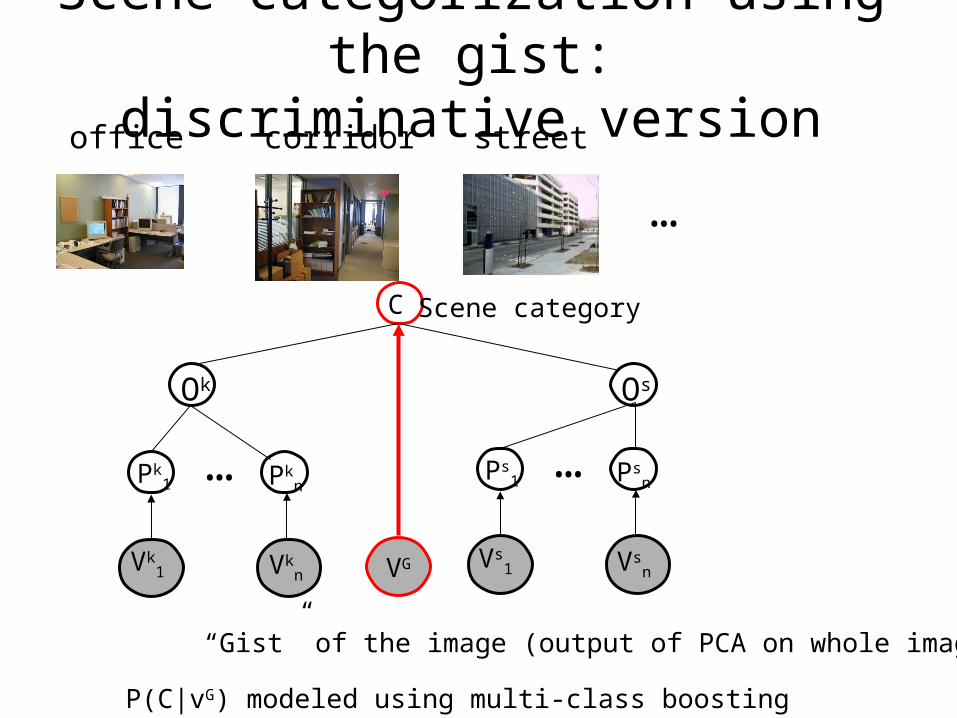
Scene categorization using the gist:discriminative version

Vkn

Pk1

Ok

Pkn

Vk1

…

C

Vsn

Ps1

Os

Psn

Vs1

…

VG

Scene category

“Gist” of the image (output of PCA on whole image)

P(C|vG) modeled using multi-class boosting

office streetcorridor

…

Scene categorization using the gist: generative version

Vkn

Pk1

Ok

Pkn

Vk1

…

C

Vsn

Ps1

Os

Psn

Vs1

…

VG

Scene category

“Gist” of the image (output of PCA on whole image)

P(vG|C) modeled using a mixture of Gaussians

office streetcorridor

…

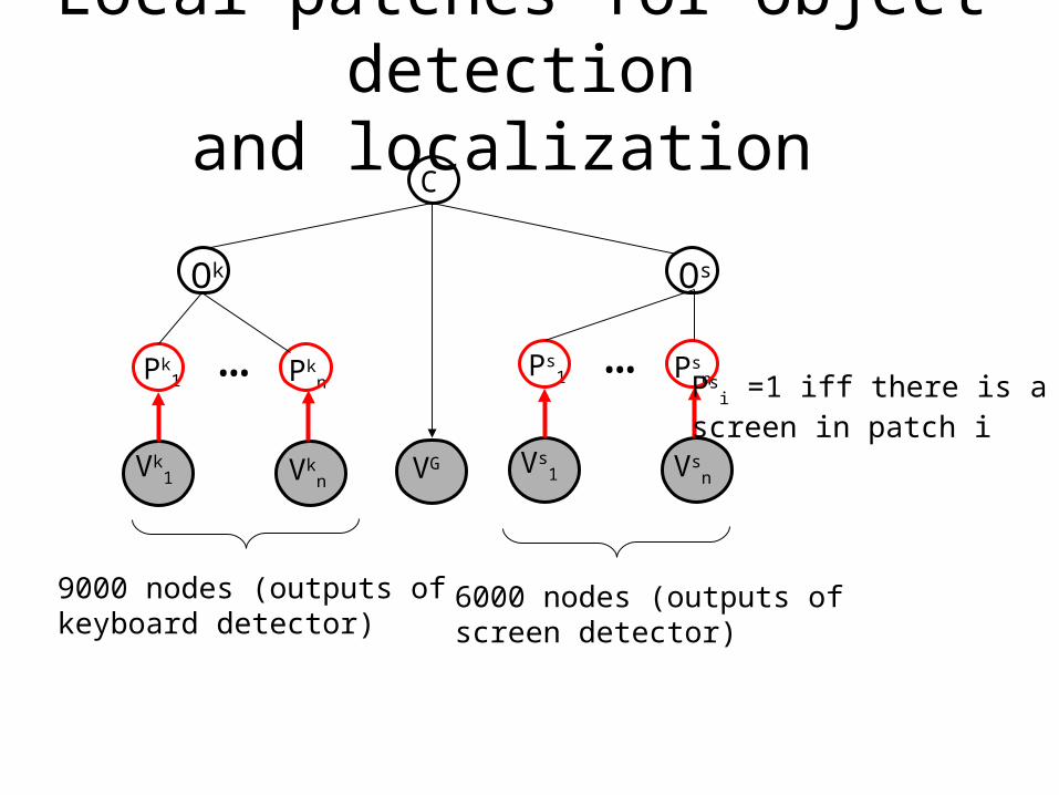
Local patches for object detectionand localization

6000 nodes (outputs ofscreen detector)

9000 nodes (outputs ofkeyboard detector)

Vkn

Pk1

Ok

Pkn

Vk1

…

C

Vsn

Ps1

Os

Psn

Vs1

…

VG

Psi =1 iff there is a

screen in patch i

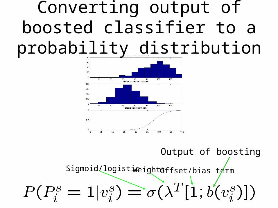
Output of boosting

Sigmoid/logistic weights Offset/bias term

Converting output of boosted classifier to a probability distribution

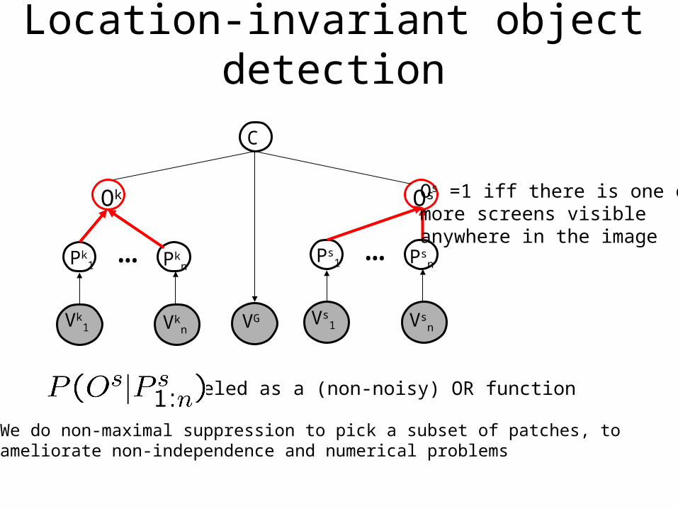
Location-invariant object detection

Vkn

Pk1

Ok

Pkn

Vk1

…

C

Vsn

Ps1

Os

Psn

Vs1

…

VG

Os =1 iff there is one ormore screens visibleanywhere in the image

Modeled as a (non-noisy) OR function

We do non-maximal suppression to pick a subset of patches, toameliorate non-independence and numerical problems

Probability of scene given objects

Vkn

Pk1

Ok

Pkn

Vk1

…

C

Vsn

Ps1

Os

Psn

Vs1

…

VG

Modeled as softmax function

Inference requires joint P(Os, Ok|vs, vk) which may be intractableProblem:

Logistic classifier

Probability of object given scene

Vkn

Pk1

Ok

Pkn

Vk1

…

C

Vsn

Ps1

Os

Psn

Vs1

…

VG

e.g., cars unlikely in an office, keyboards unlikely in a street

Naïve-Bayes classifier

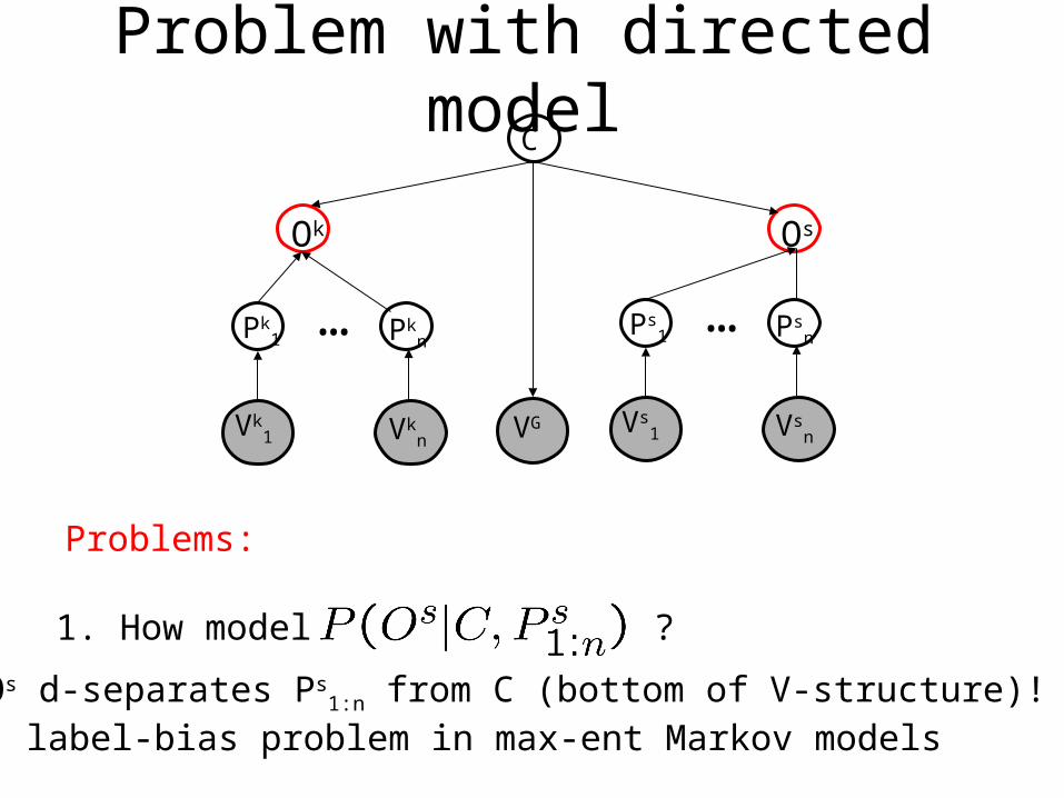
Problem with directed model

Vkn

Pk1

Ok

Pkn

Vk1

…

C

Vsn

Ps1

Os

Psn

Vs1

…

VG

Problems:

1. How model ?

2. Os d-separates Ps1:n from C (bottom of V-structure)!

c.f. label-bias problem in max-ent Markov models

Undirected model

Vkn

Pk1

Ok

Pkn

Vk1

…

C

Vsn

Ps1

Os

Psn

Vs1

…

VG

= i’th term of noisy-or

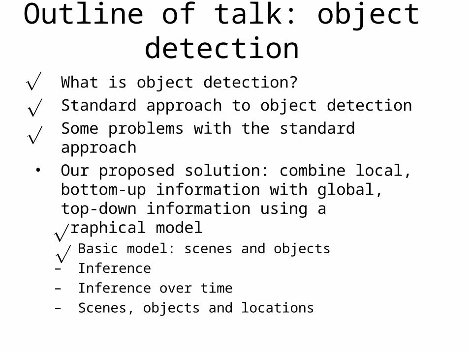
Outline of talk: object detection

• What is object detection?• Standard approach to object detection• Some problems with the standard approach• Our proposed solution: combine local,

bottom-up information with global, top-down information using a graphical model

– Basic model: scenes and objects

– Inference

– Inference over time

– Scenes, objects and locations

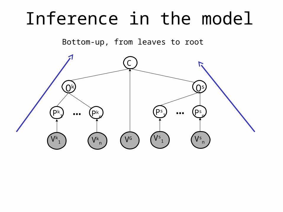
Inference in the model

Vkn

Pk1

Ok

Pkn

Vk1

…

C

Vsn

Ps1

Os

Psn

Vs1

…

VG

Bottom-up, from leaves to root

Inference in the model

Vkn

Pk1

Ok

Pkn

Vk1

…

C

Vsn

Ps1

Os

Psn

Vs1

…

VG

Top-down, from root to leaves

Adaptive message passing

• Bottom-up/ top-down message-passing schedule isexact but costly

• We would like to only run detectors if they are• likely to result in a successful detection, or• likely to inform us about the scene/ other objects (value of information criterion)

• Simple sequential greedy algorithm:1. Estimate scene based on gist2. Look for the most probable object3. Update scene estimate

4. Repeat

Outline of talk: object detection

• What is object detection?• Standard approach to object detection• Some problems with the standard approach• Our proposed solution: combine local,

bottom-up information with global, top-down information using a graphical model

– Basic model: scenes and objects

– Inference

– Inference over time

– Scenes, objects and locations

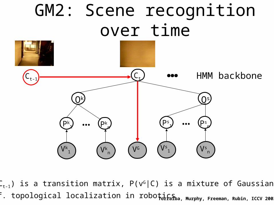
GM2: Scene recognition over time

…

Cf. topological localization in robotics

P(Ct|Ct-1) is a transition matrix, P(vG|C) is a mixture of Gaussians

Torralba, Murphy, Freeman, Rubin, ICCV 2003

Vkn

Pk1

Ok

Pkn

Vk1

…

Ct

Vsn

Ps1

Os

Psn

Vs1

…

VG

Ct-1 HMM backbone

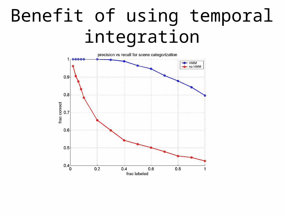
Benefit of using temporal integration

Outline of talk: object detection

• What is object detection?• Standard approach to object detection• Some problems with the standard approach• Our proposed solution: combine local,

bottom-up information with global, top-down information using a graphical model

– Basic model: scenes and objects

– Inference

– Inference over time

– Scenes, objects and locations

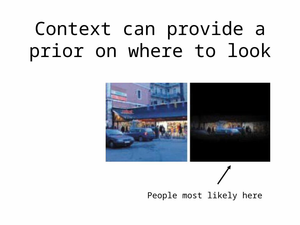
Context can provide a prior on where to look

People most likely here

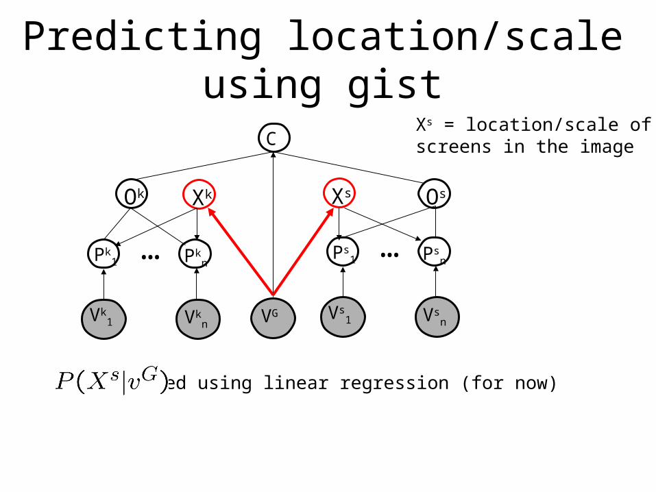
Predicting location/scale using gist

Vkn

Pk1 Pk

n

Vk1

…

C

Vsn

Ps1

Os

Psn

Vs1

…

VG

Ok Xk Xs

Xs = location/scale ofscreens in the image

modeled using linear regression (for now)

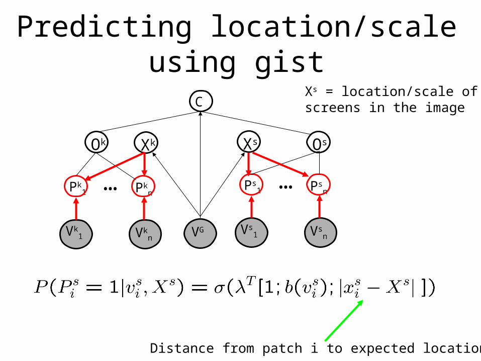
Predicting location/scale using gist

Vkn

Pk1 Pk

n

Vk1

…

C

Vsn

Ps1

Os

Psn

Vs1

…

VG

Ok Xk Xs

Xs = location/scale ofscreens in the image

Distance from patch i to expected location

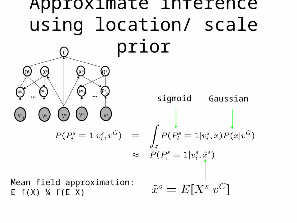
Approximate inference using location/ scale prior

Mean field approximation:E f(X) ¼ f(E X)

sigmoid Gaussian

Vkn

Pk1

Pkn

Vk1

…

C

Vsn

Ps1

Os

Psn

Vs1

…

VG

Ok Xk Xs

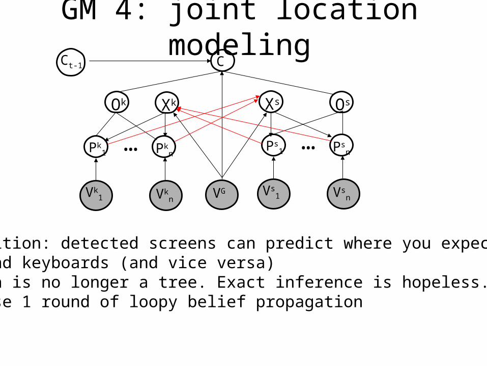
GM 4: joint location modeling

Vkn

Pk1 Pk

n

Vk1

…

C

Vsn

Ps1

Os

Psn

Vs1

…

VG

Ok Xk Xs

•Intuition: detected screens can predict where you expectto find keyboards (and vice versa)•Graph is no longer a tree. Exact inference is hopeless.•So use 1 round of loopy belief propagation

Ct-1

One round of BP for locn priming

Summary of object detection

• Models are big and hairy

• But the pain is worth it (better results)

• We need a variety of different (fast, approximate) inference algorithms

• We need parameter learning for directed and undirected, conditional and generative models

Outline of talk

• BNT

• Using graphical models (but not BNT!) for visual object recognition

• Lessons learned: my new software philosophy

My new philosophy

• Expose primitive functions• Bypass class hierarchy• Building blocks are no longer CPDs, but higher-level units of

functionality• Example functions

– learn parameters (max. likelihood or MAP)– evaluate likelihood of data– predict future data

• Example probability models– Mixtures of Gaussians– Multinomials– HMMs– MRFs with pairwise potentials

HMM toolbox

• Inference– Online filtering: forwards algo. (discrete state Kalman)– Offline smoothing: backwards algo.– Observed nodes are removed before inference, i.e., P(Qt|yt)

computed by separate routine

• Learning: – Transition matrix estimated by counting– Observation model can be arbitrary (e.g., mixture of

Gaussians)– May be estimate from fully or partially observed data

Y1 Y3

X1 X2 X3

Y2

Example: scene categorization

counts = compute_counts([place_num…]);

hmm.transmat = mk_stochastic(counts);

hmm.prior = normalize(ones(Ncat,1));

[hmm.mu, hmm.Sigma] = mixgauss_em(trainFeatures, Ncat);

Learning:

ev = mixgauss_prob(testFeatures, hmm.mu, hmm.Sigma);

belPlace = fwdback(hmm.prior, hmm.transmat, ev, 'fwd_only', 1);

Inference:

BP/MRF2 toolbox

•Estimate P(x1, …, xn | y1, …, yn)

• (xi, yi) = P(observe yi | xi): local evidence

• (xi, xj) / exp(-J(xi, xj)): compatibility matrixc.f., Ising/Potts model

Observed pixels

Latent labels

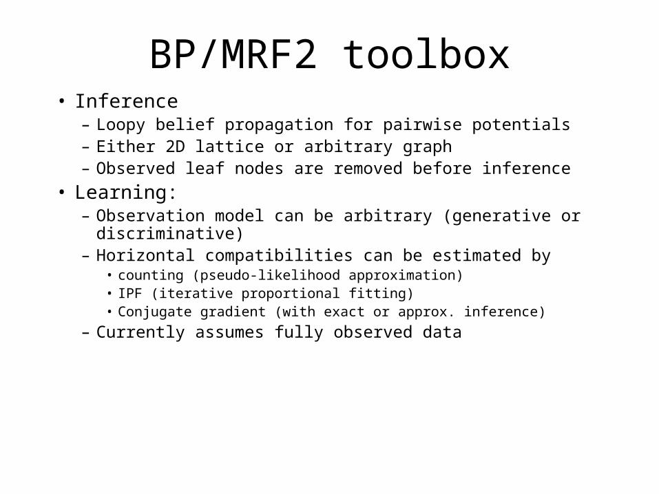
BP/MRF2 toolbox• Inference

– Loopy belief propagation for pairwise potentials– Either 2D lattice or arbitrary graph– Observed leaf nodes are removed before inference

• Learning: – Observation model can be arbitrary (generative or

discriminative)– Horizontal compatibilities can be estimated by

• counting (pseudo-likelihood approximation)• IPF (iterative proportional fitting)• Conjugate gradient (with exact or approx. inference)

– Currently assumes fully observed data

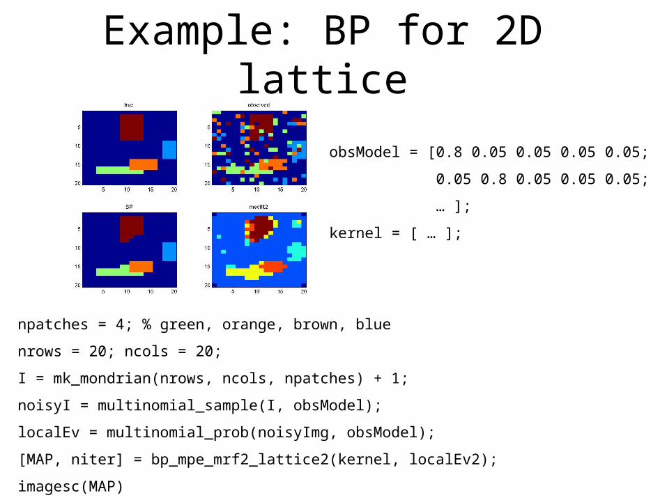
Example: BP for 2D lattice

npatches = 4; % green, orange, brown, blue

nrows = 20; ncols = 20;

I = mk_mondrian(nrows, ncols, npatches) + 1;

noisyI = multinomial_sample(I, obsModel);

localEv = multinomial_prob(noisyImg, obsModel);

[MAP, niter] = bp_mpe_mrf2_lattice2(kernel, localEv2);

imagesc(MAP)

obsModel = [0.8 0.05 0.05 0.05 0.05;

0.05 0.8 0.05 0.05 0.05;

… ];

kernel = [ … ];

Summary

• BNT is a popular package for graphical models• But it is mostly useful only for pedagogical purposes.• Other existing software is also inadequate.• Real applications of GMs need a large collection of

tools which are– Easy to combine and modify

– Allow user to make speed/accuracy tradeoffs by using different algorithms (possibly in combination)

Local patches for object detectionand localization

6000 nodes (outputs ofscreen detector)

9000 nodes (outputs ofkeyboard detector)

Vkn

Pk1

Ok

Pkn

Vk1

…

C

Vsn

Ps1

Os

Psn

Vs1

…

VG

Psi =1 iff there is a

screen in patch i

Boosted classifierapplied to patch vi

s

Logistic/sigmoid function

Problem with undirected model

Vkn

Pk1

Ok

Pkn

Vk1

…

C

Vsn

Ps1

Os

Psn

Vs1

…

VG

Problem: