the astronomical journal,119:1405 …kallrath/files/sslac2000.pdf · · 2007-02-25the...

THE ASTRONOMICAL JOURNAL, 119 :1405È1423, 2000 March2000. The American Astronomical Society. All rights reserved. Printed in U.S.A.(

ANALYSES OF THE CURRENTLY NONECLIPSING BINARY SS LACERTAE ORSS LACERTAEÏS ECLIPSES1

E. F. MILONE2Physics and Astronomy Department, University of Calgary, Calgary T2N 1N4, AB, Canada ; milone=acs.ucalgary.ca

S. J. SCHILLER2Physics Department, South Dakota State University, Box 2219, Brookings, SD 57007-0395 ; schilles=mg.sdstate.edu

U. MUNARI

Osservatorio Astronomico di Padova, Sede di Asiago, I-36012 Asiago (VI), Italy ; munari=astras.pd.astro.it

AND

J. KALLRATH

BASF-AG, ZOI/ZC-C13, D-67056 Ludwigshafen, Germany ; and Department of Astronomy, University of Florida, Gainesville, FL 32611 ;kallrath=zx.basf-ag.de, kallrath=astro.uÑ.edu

Received 1999 August 23 ; accepted 1999 November 18

ABSTRACTConÐrmatory evidence for changing light-curve amplitude of the former eclipsing and current SB2

system SS Lac in the Open Cluster NGC 7209 has been uncovered. Remeasured Harvard plate data andpublished and compiled data sets reveal that the depth of the primary minimum increased between the1890s and 1902 and decreased in the 1920s and 1930s. A parabolic Ðtting of the amplitude with phasepredicts a maximum at 1911.5, with an eclipse onset at 1885.3 and eclipse cessation at 1937.8. WeconÐrm the Ðnding of Lehmann, that the systemÏs inclination varies with time and that a central eclipseoccurred D1912, and we concur with Mossakovskaya that eclipses e†ectively ceased D1940. Estimatesof SS Lac on plates taken at Tashkent between 1937 and 1940 further serve to conÐrm the result. Thus,SS Lac belongs to a small but elite class of triple systems in which changes due to dynamical e†ects canbe seen over a single human lifetime. In order to explore the properties of the SS Lac system, recentradial velocity curves and archival photographic and visual light curves have been analyzed with ver-sions of the Wilson-Devinney code, augmented with a simplex routine to test solution uniqueness. Themodeling solutions for the Dugan-Wright light curves ostensibly indicate that the former eclipsingsystem is composed of two early A stars of only slightly di†ering masses (2.57 ^ 0.16 and 2.59 ^ 0.19

and e†ective surface temperatures (8750^ 300 [assumed for component 1] and 8542^ 309 K), butM_

)signiÐcantly di†erent radii (2.38^ 0.02 and 3.63^ 0.07 and luminosities (30^ 4 and 63^ 9 forR

_) L

_)

the hotter and cooler components, respectively. The light-curve solutions are compromised somewhat byvariable eclipse depths over the ranges of dates of the data sets. This is especially true of the most com-plete light curve, that of Dugan & Wright ; the others also su†er from incompleteness (that ofWachmann) and high scatter (that of Kordylewski, Pagaczewski, & Szafraniec). As a consequence, small,temporal variations in such system properties as the eccentricity, argument of periastron, modiÐed Rochepotentials, luminosities, and third light level, cannot be ruled out from currently available data. However,solutions with WD95, a self-iterating, dampedÈleast squares version of the Wilson-Devinney program,reveal optimized inclinations for the data sets that project an inclination variation of yr~1, but no0¡.16evidence of apsidal motion. We Ðnd a distance for the system of 898 ^ 95 pc, consistent with the valueof et al. of 1040 ^ 10 pc, and Ðnally, on the bases of location on the sky, proper motion,Vansevic— iusradial velocity, photometry, and properties deduced in the present study, we conÐrm its membership inthe cluster NGC 7209.Key words : binaries : eclipsing È binaries : spectroscopic È star clusters : individual (NGC 7209) È

stars : individual (SS Lacertae)

1. INTRODUCTION

The discovery of variability of SS Lacertae(BD]45¡3782) is attributed to Henrietta Leavitt by Pick-ering (1907). Shapley & Swope (1938) state that the light-curve analysis presented by Dugan & Wright (1935)is ““ based on Miss WrightÏs measures on Harvard photo-graphs.ÏÏ The Ðrst light curve, based on visual estimates, waspublished by Ho†meister (1921) and subsequent photogra-phic light curves were reported by Dugan & Wright (1935)

ÈÈÈÈÈÈÈÈÈÈÈÈÈÈÈ1 Publications of the Rothney Astrophysical Observatory, No. 73.2 Visiting Astronomer, Dominion Astrophysical Observatory.

and by Wachmann (1935, 1936). Another set of potentiallyusable light curves is given by Kordylewski, Pagaczewski, &Szafraniec (1961). Ho†meister derived a very short periodfor the system, 1.201499 days, and a sinusoidal term for theephemeris. The subsequent work by Dugan & Wright(1935) revealed a period of 14.41629 days, a result conÐrmedby Wachmann (1936).

The system was observed photometrically and spectro-scopically in the early 1980s by S. J. S. as part of his Ph.D.thesis work on binaries in clusters, supplemented by addi-tional photoelectric observations at the Rothney Astro-physical Observatory (RAO) in the interval 1989È1991. Thesystem was a strong candidate for membership in the opencluster NGC 7209 and thus for the binaries-in-clusters

1405

1406 MILONE ET AL. Vol. 119

program at the University of Calgary. Cluster membershipwas suggested by several factors : proximity on the sky,proper motions, and radial velocity studies. Artiukhina(1961), Lavdovska (1962), van Schewick (1966), and Platais(1991) all identify SS Lac as a probable member on the basisof proper motions. As we note later, radial velocities alsosupport membership. Finally, the variable lies near the blueturno† of the cluster color-magnitude diagram (Hoag et al.1961) where SS Lac is identiÐed as star 4. The latter circum-stance indicated SS Lac to be a suitable candidate to yieldcluster turno† masses and the evolutionary states of thecomponents.

Although SS Lac has been included often in lists ofapsidal motion candidates, no Ðrm evidence for apsidalmotion in this system has been found (Dugan & Wright1937) other than the suspicion that it could be presentbecause of a slight orbital eccentricity. Given the absence ofsuch motion over a 45 yr interval, Shapley & Swope (1938)suggested that the apsidal period was probably ““ tens ofthousands of years.ÏÏ

The S. J. S. photoelectric photometry of 1981 and 1982 (atRAO), in 1982È1983 (at McDonald and Table MountainObservatories), and in the years 1989È1991 (at RAO),revealed no sign of an eclipse. Negative results have beenreported also by Zakirov & Azimov (1990), Schiller et al.(1991), Schiller & Milone (1996), and Mossakovskaya(1993).

From photographic archive examination, Moss-akovskaya (1993) concluded that the cessation of eclipses inSS Lac had occurred between the mid-1930s and the 1940s,although a limit in the 1950s was suggested initially byZakirov & Azimov (1990). Lehmann (1991) suggested thatthe eclipses became progressively shallower prior to cessa-tion. In the present paper, we examine this hypothesis andpresent evidence that strengthens his conclusion.

The presence of a binary with at least one variable orbitalproperty in an open cluster raises the possibility of anencounter with another cluster member. The probability forsuch an encounter is low but certainly not zero. Conse-quently, the possibility of dynamical interaction makes it ofinterest to understand better the properties of the systemand individual stars involved and to investigate such vari-able eclipse conditions as the dates of eclipse onset andcessation. These were the purposes of the present study.Spectroscopic observations were obtained by S. J. S. forradial velocity analysis in the mid-1980s. In these spectra,no strong evidence of duplicity could be discerned either inor outside of the Balmer lines, which strongly dominate thespectrum. Most recently, however, Tomasella & Munari(1998) have been successful in detecting the lines of bothcomponents in higher signal-to-noise ratio (S/N) and higherresolution echelle spectra from Asiago. In their study, onlythe Balmer lines Ha, Hb, and Hc were used to determineradial velocities. Tomasella & Munari (1998) analyzed theirradial velocity curves and obtained a set of spectroscopicelements.

Our previous analysis e†orts (Milone, Stagg, & Schiller1992b) involved only the mean light curve of Dugan &Wright without beneÐt of the spectroscopic solution. Subse-quently, we have reanalyzed these data, those of Wachmann(1936), and a set of visual estimates of Kordylewski(Kordylewski et al. 1961), making use of the radial velocitiesto delimit properties of the system. The analysis of all avail-able data sets marks an attempt to constrain the variation

of the systemÏs properties and to investigate the changingamplitude of the light variation with time.

This is not the Ðrst time that eclipse cessation has beenseen. The visibility of eclipses depends upon the sizes of theeclipsing and eclipsed objects, the inclination of the orbitalplane, and, in eccentric orbit cases, the eccentricity andorientation of the line of apsides. Occulting disks or shellsare known to vary in size, and, usually on evolutionarytimescales, and so may the stellar components themselves.Systems in which eclipse amplitude has been observed tovary include IU Aur (Harries, Hilditch, & Hill 1998 ; Schiller1981), RW Per (Schaefer & Fried 1991), and, most recently,V907 Sco (Sandberg Lacy, Helt, & Vaz 1999), in whichchanging eclipse amplitudes have been attributed to thevarying of the eclipsing binary orbital plane relative to theinvariable plane involving the close binary and a moredistant third star.

Among these other systems, the only one with possible(although disputed) cluster membership that has periodiceclipse seasons is V907 Sco (Sandberg Lacy et al. 1999). Wewill discuss the properties of the third component in the SSLac system in ° 4.

2. DATA

2.1. Photometric DataPhotometric observations were obtained with the

automated, gated pulse-counting photoelectric photometrysystem (RADS) on the 41 cm telescope of the RothneyAstrophysical Observatory (see Milone et al. 1982 ; Milone& Robb 1983). Observations were made in U, B, V Johnsonand R and I Cousins passbands relative to comparison starBD ]45¡3771 \ SAO 51588 \ HD 209482 in the 1982È1983 seasons and relative to comparison star BD]45¡3777 \ SAO 51617 \ HD 209692 in the 1989È1991seasons.

As with other RADS data, mean extinction coefficientshave been found to be sufficiently accurate over the smallrange of secondary mirror chop (for SS Lac and the com-parison star used in the 1990s, only D7@), because of thetypically small di†erential air mass (in this case, [0.0015P).Mean transformation coefficients were also applied, butzero points were not determined. The phasing was donewith the elements of Dugan & Wright (1935) : E0\2,415,900.76 and P\ 14.41629 days, but for photometricpurposes, phasing in the present era di†ers not at all fromphasing with the recent ephemeris, that of Tomasella &Munari (1998), cited above. The mean values of the di†eren-tial light curves for the interval JD 2,447,666È2,448,559(1989È1991 seasons) are given in Table 1. Normalized lightcurves for the 1982È1983 and 1989È1991 seasons are shownin Figure 1, where they can be compared to the photogra-phic light curve obtained by remeasurement of HarvardCollege Observatory (HCO) plates by S. J. S.

The mean values together with the absolute photometryof Hoag et al. (1961) for HD 209692 (V \ 8.53,B[V \ 0.34, U[B\ 0.16) were added to our di†erentialdata to yield mean values of the SS Lac system in the 1990sof V \ 10.049^ 0.005, B[V \ 0.169^ 0.006, andU[B\ 0.129^ 0.006, where a mean standard error(m.s.e.) of ^0.005 has been assumed for the comparison starphotometry. Standardization done by S. J. S. in the courseof photometry carried out at the MacDonald Observatory(Schiller & Milone 1987) gave the following values

No. 3, 2000 SS LACERTAE 1407

TABLE 1

SS LACERTAE RAO DIFFERENTIAL PHOTOELECTRIC MEANS

Magnitude/CI 1989 1990 1991 1989È1991

V . . . . . . . . . . . . . . 1.537 ^ 0.005 1.505 ^ 0.003 1.524 ^ 0.002 1.519 ^ 0.002N

V. . . . . . . . . . . . 14 49 77 140

B[V . . . . . . . . . . [0.171 ^ 0.008 [0.162 ^ 0.009 [0.172 ^ 0.006 [0.171 ^ 0.004N

B~V. . . . . . . . . . 14 48 75 137

U[B . . . . . . . . . [0.046 ^ 0.010 [0.029 ^ 0.007 [0.031 ^ 0.032 [0.031 ^ 0.004N

U~B. . . . . . . . . . 13 45 73 131

V [R . . . . . . . . . [0.096 ^ 0.004 [0.087 ^ 0.003 [0.087 ^ 0.002 [0.088 ^ 0.001N

V~R. . . . . . . . . 15 49 77 141

V [I . . . . . . . . . . [0.144 ^ 0.007 [0.139 ^ 0.004 [0.139 ^ 0.002 [0.140 ^ 0.002N

V~I. . . . . . . . . . 15 47 76 138

for comparison star BD ]45¡3771 : V \ 9.125^ 0.018, B[V \ 0.103^ 0.006, U[B\ 0.101^ 0.009,V [R\ 0.070^ 0.003, R[I\ 0.078^ 0.003, andV [I\ 0.138^ 0.005. S. J. S. has computed mean SS Lacphotometry for the 1982È1983 seasons : V \ 10.103^ 0.014, B[V \ 0.166^ 0.005, U[B\ 0.157^ 0.007,V [R\ 0.099^ 0.001, R[I\ 0.107^ 0.005, and V [I\0.202^ 0.004. To these we can add the photoelectric deter-minations of Lacy (1992) : V \ 10.096^ 0.006,B[V \ 0.160^ 0.003, U[B\ 0.173^ 0.006, and N \ 7,over the two seasons 1989È1990, centered at JD 2,447,822,D1989.8.

The weighted means of the three sets of UBV determi-nations are SV T \ 10.071^ 0.017, SB[V T \ 0.163^ 0.003, and SU[BT \ 0.143^ 0.010. The dispersion inV among the determinations provides mild evidencefor small brightness variation in the system over a decade,but systematic e†ects in the more recent RAO photometryare more likely reasons for the di†erences, especially sincethe epochs of the S. J. S. and Lacy determinations, which arein relative agreement, are about a decade apart. Theweighted means for these two sets alone areSV T \ 10.097^ 0.003, SB[V T \ 0.162^ 0.003, andSU[BT \ 0.166^ 0.009. These values are close to thosereported by Hoag et al. (1961), themselves, for SS Lac, theirstar 4 : V \ 10.09, B[V \ 0.14, and U[B\ 0.16 fromphotoelectric photometry. Thus, SBT \ 10.259^ 0.004 forthe system. These means have been adopted for the calcu-lation of the absolute parameters of the SS Lac system.

The lack of eclipses in historically recent times requiresany light-curve analysis to be carried out on earlier lightcurves. Literature searches for previous observations were

carried out by Zakirov & Azimov (1990), who suggestedeclipse cessation by the early 1950s, and by Mossakovskaya(1993), who concluded that eclipses must have ceasedbetween 1935 and 1940. The archival data sets include thefollowing :

1. Harvard College Observatory patrol camera plates ;individual measures have not been published (see Dugan &Wright 1935) ; 1700 plates contained usable images of SSLac. Of these, 790 plates had plate scales of 163A mm~1 orbetter, and, of these 790 plates, 591 I-series plates takenbetween 1890 and 1939 were remeasured by Schiller,Bridges, & Clifton (1996).

2. 318 visual estimates by Ho†meister at Sonnebergcovering 293 nights between 1915 May 15 and 1918October 31 ; unfortunately, only times of minimum, and aninteresting sinusoidal ephemeris, were published.

3. 197 Bergedorf Observatory plates taken between 1929May and 1932 December measured by Wachmann with aLeitz Double Microscope (Wachmann 1935, 1936).

4. 523 visual estimates with mainly f/11 or f/12 20 cmobjective telescopes at Cracow and Warsaw between 1927May and 1937 October (Kordylewski et al. 1961).

5. 25 plates taken with f/4.5 120 mm cameras of theEngelhardt Observatory between 1926 and 1932(Nekrasova 1938).

6. Plates taken at the Crimean station of the SternbergInstitute with a 40 cm astrograph and from the Moscowstation at Krasnoi Presne with f/6.6 9.7 cm and f/5 16 cmcameras (Mossakovskaya 1993) ; they cover the intervals (a)1898 DecemberÈ1911 August (26 plates) ; (b) 1935 AugustÈ1942 November (30 plates) ; (c) 1950 OctoberÈ1957 Septem-

FIG. 1.ÈPhotometry of SS Lacertae. L eft, The light curve from a portion of the Harvard College Observatory database of plates remeasured by S. J. S. ;right, photoelectric observations in the V passband for the 1982È1983 and 1989È1991 observing seasons, demonstrating the absence of eclipses in the modernera.


ber (40 plates) ; and (d) Sporadically through the interval1968 SeptemberÈ1987 October (185 plates).

7. Sonneberg Sternwarte patrol camera plates takenbetween 1890 and 1989 (described by Lehmann 1991).These results have not been available generally and havenot been used in the present study.

8. Finally, there is the published report of Tashpulatov(1965), who listed from 983 estimates from plates taken atthe Tashkent Astronomical Observatory covering the range1937 AugustÈ1955 May. We discuss these data and morerecent estimates from them at length below.

There are problems with the archival data. Dugan &Wright (1935) published neither tables of their mean andraw light curves nor a diary of the individual plates. TheWachmann (1936) data, which are the most homogeneousin both time interval and light-curve scatter, lacks data onthe falling branch and deep minimum of the secondaryeclipse. Ho†meister (1921) does not list any light curve mea-surements, while those of Kordylewski, Pagaczewski, &Szafraniec (1961) su†er from large scatter. No otherpublished data set, except that of Tashpulatov (1965), whichwe discuss below, shows eclipses.

The normal points data plotted by Dugan & Wright(1935) were scanned by E. F. M. with an HPC-4 scanner athigh resolution, printed at higher magniÐcation, and mea-sured with a Data Scales Inc. Variable Rule. Errors due todistortion and mismeasurement are judged to be no morethan the uncertainty in the placement of the original datapoints, estimated at mag, and in phase. Only[0.02 [0.002the second of two plottings of the primary minimum in theÐgure given by Dugan & Wright (1935) is symmetric and sothese points were used for the Ðnal analysis. These mea-sured and rescaled data, and others described here, areavailable on request in spreadsheet format. The measuredvalues were then normalized to the mean of the data outsidethe minima, On the advice of ourSmpgmaxT \ 10.289^ 0.002.referee, we have included the phased and normalized remea-sured data as an aid to the reader.

To check the validity of the Dugan & Wright (1935) plotand to search for clues to the past behavior of the SS Lacsystem, Schiller et al. (1996) imaged all relevant plates withwell-resolved images in the plate stacks at the HarvardCollege Observatory with a CCD video camera and framegrabber coupled to a 0.7] 3.0 zoom microscope to producefor each plate image an eight-bit digitized record over a Ðeldof 512 ] 512 pixels. The magniÐcation permitted the com-parison stars to be imaged on the higher resolution platesand subsequently measured. The plates with lower platescales (D400AÈ700A mm~1) were imaged but not measuredbecause blending due to overcrowding on those plates mademagnitude determination uncertain. Up to 16 stars weremeasured on each frame, but, depending on the degree towhich seeing merged the images, between 8 and 12 wereused for the di†erential photographic photometry. Thecomparison stars are listed in Table 2.

The HCO data sets, including that of Schiller et al. (1996),were normalized to the mean maximum value. For light-curve purposes, the latter data set was used to check meanlight levels and to verify the placements of the minima. TheDugan & Wright mean data (hereafter DW35), plotted inunits of days, were phased with the most recent elements(Tomasella & Munari 1998) : andP0 \ 14.41638 E0\2450716.32.

TABLE 2

COMPARISON STARS USED FOR THE HARVARD PLATE

MEASURESa

X Y V ID

[23.10 . . . . . . [15.88 8.53 BD ]45¡3771]2.70 . . . . . . . [8.57 10.26]0.70 . . . . . . . [10.87 10.57[1.95 . . . . . . . [6.30 10.61[10.36 . . . . . . ]5.59 10.68[1.65 . . . . . . . [2.73 10.68[6.62 . . . . . . . [6.82 10.75[6.29 . . . . . . . [11.17 10.95[16.41 . . . . . . [12.14 11.01[0.45 . . . . . . . [10.54 11.08[13.96 . . . . . . [10.17 11.11]8.46 . . . . . . . [3.82 11.37[5.87 . . . . . . . ]4.44 11.39[4.69 . . . . . . . [2.48 11.73[9.34 . . . . . . . [12.31 11.84[4.15 . . . . . . . [0.63 12.01

a Relative frame position and magnitude data fromHoag et al. 1961.

The remeasured HCO data demonstrate the presence ofeclipses of large (D0.6 mag), but also possibly varying,amplitude. A plot is shown in Figure 1a. S. J. S. found that55 of the measured plates occur within 0.015P of mideclipse(for the analysis described in ° 4, this condition was slightlyrelaxed to allow for the possibility of phase variation in thetimes of minima; we record 61 low-light entries). Of the 55,37 are in the primary minimum, with 29 taken between 1890and 1903, six between 1906 and 1907, and the remainingtwo in 1933. Of the 18 secondary minimum plates, 11occurred before 1907 and six after 1923. The phases ofminimum and maximum appear as in Dugan & Wright(1935) ; the primary minimum depth appears deeper herethan in the Dugan & Wright (1935) normal points lightcurve, although the scatter is large. When all the data areconsidered, it is clear that the shape and depth of the meanplot of Dugan & Wright (1935) represent a composite of afamily of light curves. The details of the cycle-by-cyclevariation of the light curve revealed in the plate remeasuresare in themselves interesting, and we will discuss them in ° 4.

The HCO collection contains 90 plates of SS Lac atminimum, according to Dugan & Wright (1935). Since theremeasured set contains, in our current tally, only 61 low-light values, an important proportion of these data, albeitmostly from plates with less favorable plate scales, are stillunavailable.

In contrast to the paucity of observational details givenby Dugan & Wright, Wachmann (1936) conveniently pro-vided mean and individual Bergedorf plate data, as well as aplot of the mean data. This is an invaluable set of high-quality data from a limited range of dates, permitting com-parisons between early and late epoch properties of thesystem. Unfortunately, although the minima are certainlydiscernible, they are not so well covered as in the Dugan &Wright (1935) paper, especially the secondary minimum inwhich there are no points on the falling branch and onlythree on the rising branch. The individual observations ofthe Wachmann mean data set (hereafter W36), whichincluded HJD values, were rephased with the Tomasella &Munari (1998) elements.


At one stage, the data of Wachmann (1936) were com-bined and modeled together with the Dugan & Wright datain order to obtain fuller light curve coverage since the rangeof dates spanned by the two sets overlap (Milone & Schiller1998). However, subsequent work revealed that modeling isbetter carried out on the individual sets : Ðrst, because of aslight phasing o†set between the two sets of data resultingin an apparent widening of the primary minimum in thecombined set, and second, because of the e†ectively di†erentmean light-curve properties encompassed by the two sets ofdata. Wachmann (1936) himself commented on the appar-ent phase shift (D0.1 day) between his minimum and that inthe Dugan & Wright (1935) epoch and was puzzled by it,given the large range of dates of the plates that were used byDugan & Wright (1935) to obtain their mean light curve. Asa consequence, in the present analyses the data sets havebeen treated separately. The tabulated individual obser-vations as well as the mean data values of Wachmann werenormalized (to 9.998, in maximum light).

The data published in Kordylewski et al. (1961) overlapthose of Wachmann. The Szafraniec compilation is the onlycurrently available set of nonphotographic data thatinclude eclipse observations. Of these, SzafraniecÏs ownobservations are few; the 114 visual estimations of Pagac-zewski have a m.s.e. of a single observation, atp1\ 0.088maximum light ; and KordylewskiÏs 402 estimates have

(again deduced from the residuals about thep1\ 0.065mean at maximum light phases). Both the Pagaczewski andKordylewski sets were examined for low-light values, butKordylewskiÏs larger and less noisy data set (hereafter K)was used for visual light-curve modeling trials. The datawere normalized to maximum light and means were takenof every 10 data points at maximum light ; the m.s.e. of themeans were used to compute light-curve weights for themodeling.

The list published by Tashpulatov (1965) contains faintmagnitude estimates for several minima. The last deepminimum (D0.5 mag below maximum) is given for JD2,423,200, in 1949. He included a mean light curve thatshows relatively low scatter and that disagrees with those ofDugan & Wright (1935) and Wachmann (1936) only in theamplitude of the variation, which he gave as 0.52(Tashpulatov 1965), versus 0.41 mag in the other twosources. In contrast, the data sets examined by Moss-akovskaya (1993) show very few faint data points after the1930s. Indeed, Mossakovskaya (1993) considered the entireset of data presented by Tashpulatov (1965) to be unreliableand excluded it from her own analysis. According to M.Zakirov (1998, private communication), reliable estimatesfrom the Tashkent plates are difficult to make because ofthe low plate scale of the camera and the fact that the clusterlies near the edge of many of the plates ; nevertheless, aseries of plate estimates recently made by I. M. Ischenko hasbeen kindly provided by M. Zakirov (1998, privatecommunication). They span the interval 1937È1950 andconÐrm that no minima can be attributed with any degreeof certainty to the system after 1937. We will discuss theseestimates further in ° 4.

As noted, each of the archival light curves presentsimpediments to analysis : the DW35 data are complete butare averaged over too great a range of dates to establish aunique and reliable inclination, for example. The scatter inremeasured HCO data over limited ranges of dates is toogreat to yield results signiÐcant enough to throw much

additional light on the modeled parameters (although thelevel of scatter is interesting in itself and will be discussed in° 4). The W36 data set su†ers from an incomplete secondaryminimum, and the Kordylewski et al. (1961) sets have toohigh scatter for precise determinations of most parameters.Nevertheless, the data sets DW35, W36, and K are the onlylight-curve data usable for the analyses described in the nextsection, and so we attempt to analyze them as fully as pos-sible. Independently of the light-curve analysis, minima inthe full data sets of the remeasured Harvard archival data,and in other published data, have been examined, resultingin a characterization of the variation of the depth of theminima.

2.2. SpectroscopyRadial velocity observations of SS Lac were made by

S. J. S. in 1983È1984 at DAO with the 1.8 m telescope with asingle-stage image-intensiÐer and both photographic platesand Reticon detector. Twelve observations were obtainedwith 15 mm~1 nominal reciprocal linear dispersion. TheA�data were reduced and analyzed with the REDUCE andVCROSS software of Hill, Fisher, & Poeckert (1982) andHill (1982), respectively. The cross-correlated radial veloci-ties are given with respect to comparison star HD 27962(A3 V or A2 IV) ; d Tau, the radial velocity of which Wilson(1963, p. 52) gives as ]34.7 km s~1. The results of this Ðrstspectroscopic work were reported by Schiller & Milone(1996) to be negative, in the sense that the radial velocity didnot appear to vary signiÐcantly from the gamma velocity,which was determined to be [24.9^ 4.8 km s~1 (excludingthe datum from plate 92593, discrepant from the others buttaken at nearly the same phase as another point close to theaverage). These data are summarized in Table 3. Thephasing is that of Dugan & Wright (1935).

Subsequently, Etzel et al. (1996), Etzel & Vogelnau (1996),and Stefanik et al. (1996) reported a clear doubling of thelines, and Tomasella & Munari (1998) produced a radialvelocity curve for each component. The mean value ofSchiller & Milone (1996) is not signiÐcantly di†erent fromeither the gamma velocity determined here ([19.9^ 0.8) orby Tomasella & Munari (1998) ([21.2^ 0.3) or the valuefor a third component seen at quadratures ([22.3^ 3.0 kms~1) found by Tomasella & Munari (1998).

P. B. Etzel (1998, private communication) reports that thedoubling of lines is seen in metal lines in the blue region of

TABLE 3

SS LACERTAE ARCHIVAL RADIAL VELOCITY DATA

Plate HJD Phasea RVb

91997 . . . . . . 2,445,546.9615 0.438 [69.0491998 . . . . . . 2,445,546.9878 0.439 [60.9892004 . . . . . . 2,445,547.7552 0.493 [52.5292012 . . . . . . 2,445,548.7587 0.562 [63.8592014 . . . . . . 2,445,548.7670 0.563 [54.2692593 . . . . . . 2,445,710.6806 0.794 [33.8692954 . . . . . . 2,445,710.6895 0.795 [58.8192957 . . . . . . 2,445,711.6562 0.862 [59.5493370 . . . . . . 2,445,918.8792 0.236 [60.2693371 . . . . . . 2,445,918.8882 0.237 [53.3493372 . . . . . . 2,445,918.8988 0.237 [51.1593380 . . . . . . 2,445,919.0257 0.246 [62.64

a Phased as per Dugan & Wright 1935.b Relative to HD 27962.


the spectrum. Tomasella & Munari (1998) measured theradial velocity variation only in the Balmer lines in theirechelle spectra, which covered the range from Ha to Hc,because the weakness of the other lines precluded reliablemeasurements from them.

A reexamination of tracings of the spectra obtained byS. J. S. does not reveal any clear-cut evidence of this doub-ling even in the Balmer lines, which were systematicallymasked o† for the cross-correlation procedure (a standardpractice because inclusion of the broad and often blendedBalmer lines tends to broaden rather than sharpen CCFpeaks), although a suggestion is present in some cases. Thedoubling is certainly visible in the cores of the Balmer linesof spectra taken subsequently at DAO with the samecamera on DAOÏS 1.8 m telescope with unintensiÐed CCDdetectors. These new spectra are not reduced at presentwriting, but the separations of the cores at quadratures doconÐrm the results of Tomasella & Munari (1998) andothers. Thus, our earlier failure to detect doubling can beattributed to insufficient S/N possibly coupled withresolution problems in our data.

The spectra also provide temperature estimates that areneeded for light-curve modeling. Tracings of our DAOspectra (which reveal weak lines of jj4227 and 4233, as wellas other metal lines and a depth of the Ca K line that ofD23Ca H ] Hv) suggest a spectral type between A3 and A4,while Tomasella & Munari (1998), on the basis of the strongwings of the Balmer lines, suggest A2. The temperature scaletabulated by Popper (1980) was used to provide tem-perature estimates. With initial temperature values for bothspectral type estimates (i.e., A3.5 and A2) and adjustedT2with the temperature di†erence found from preliminarymodeling trials of the DW35 data, a best value of T1\ 8732K, just slightly cooler than the temperature scale predictsfor an A2 classiÐcation, was obtained. However, this resultwas derived for models which were not fully consist with theinformation supplied by Tomasella & Munari (1998). Con-sequently, for most of the Ðnal modeling, which is describedbelow, was adopted, appropriate for a star of A2T1\ 8750spectral class (Popper 1980). We next describe the analysisof the Tomasella & Munari (1998) data with our light andvelocity modeling program, WD93K93.

3. ANALYSES

3.1. Radial V elocity AnalysesTo begin the analyses, the radial velocity data of Toma-

sella & Munari (1998, hereafter TM98) were reanalyzedwith WD93K93c, a University of Calgary version of theWilson-Devinney (WD) program. All light and radial veloc-ity curves were modeled in mode 2, appropriate fordetached systems. Albedo and gravity-darkening coeffi-cients were set at 1.0 for these early-type stars with pre-sumed radiative envelopes, and the atmospheres optionwith Kurucz (1993) atmospheres for the component starswas invoked for all trials. Solar [Fe/H] values wereassumed, and given the relatively low quality of theanalyzed light-curve data, no other compositions wereexplored. All models indicate that the stars are well separ-ated with negligible radiative interaction. Consequently,simple (single-pass) reÑection was used for all modeling.

The procedure was as follows : The radial velocity curveof each component was analyzed separately to convergence,yielding consistent values of the parameters (the bary-Vc

centric velocity) and Pshift (phase shift). The latter is thephase increment to a synthetic light curve required to matchthe phasing of the observations.

The RV curves were then modeled together. The initialparameters (in the Wilson 1992 conventions) were thosedetermined by TM98, viz., the projected semimajor axis insolar radii, a sin i \ 42.5 ; eccentricity, e\ 0.122 ; argumentof periastron, u\ 332¡ ; the barycentric velocity, Vc \[21.2 km s~1 ; and mass ratio, Inq \M2/M1\ 1.041.addition, Pshift or */ was assumed to be zero initially, andthe inclination, i, was Ðxed at 78¡ as per TM98. Theassumed photometric parameters were the preliminary setdetermined by Milone & Schiller (1998) for the Dugan-Wright data. The data were weighted by the inverse of theerror cited in TM98, but with zero weight given data justoutside the conjunctions, where blending may have been aproblem. Data at the conjunctions were given full weight.

A critical step for analysis is the identiÐcation of the stareclipsed at primary minimum (phase 0.0), star 1 in Wilson-Devinney usage, with the TM98 star ““ b.ÏÏ Star 2 is thusTM98Ïs star ““ a.ÏÏ The radial velocity and spectral plots ofTM98 leave no doubt that this is the case. In all modeling,Pshift (applied to the computed light curve) was adjusted.Other adjusted parameters were a, e, u, q, and AdoptedVc.and unadjusted values for some of the other parameters aregiven along with the RV-Ðtting results in Table 4 ; the Ðttingresults can be seen in Figure 2.

While not identical (the parameters were started at theTM98 values and consistently moved to new values in alltrials), the parameters are seen to be not signiÐcantly di†er-ent from those of Tomasella & Munari (1998), but theformal uncertainty in a single RV datum of average weight,equivalent to the uncertainty in the RV curve Ðtting, islarger (^4 vs. ^0.8 km s~1). The phasing with the period ofTomasella & Munari (1998) is essentially consistent withminima as computed with the Dugan & Wright (1935)ephemeris ; low-light data in the minima seem to be wellphased in the remeasured HCO data, for instance. Conse-quently, no new determination of phase elements wasattempted. The phasing is such that at phase 0.00 the starundergoing eclipse (star 1 in the Wilson-Devinneyconvention) is the less massive star (star b of Tomasella &Munari 1998). Thus, q [ 1.

Following each of the iterations, the RV modeling resultswere tested with the simplex option in our code, whichautomatically iterates until the stopping criteria are met :when either the Ðtting error or each parameter errordecreases to a speciÐed target level, or when the maximum

FIG. 2.ÈRadial velocity curve Ðtting. The data of Tomasella & Munari(1998) are shown, with the Wilson-Devinney model Ðtting.


TABLE 4

SS LACERTAE RADIAL VELOCITY SOLUTIONSa

Parameter (Units) WD Analysisb WD Analysis (i Optimized)b TM98c(1) (2) (3) (4)

a (R_

) . . . . . . . . . . . . . 43.06 ^ 0.84 43.32 ^ 0.84 42.5 ^ 0.5e . . . . . . . . . . . . . . . . . . . 0.122 ^ 0.017 0.122 ^ 0.017 0.122 ^ 0.019u (deg) . . . . . . . . . . . . 353.8 ^ 6.4 353.9 ^ 9.4 332 ^ 9*/ (P) . . . . . . . . . . . . . 0.0072 ^ 0.0029 0.0072 ^ 0.0029 . . .Vc (km s~1) . . . . . . . [19.85 ^ 0.82 [19.85 ^ 0.82 [21.3 ^ 0.3q . . . . . . . . . . . . . . . . . . . 1.00830 ^ 0.03538 1.00868 ^ 0.03537 1.038 ^ 0.022i (deg) . . . . . . . . . . . . . 78.0d 76.5 78.0T1 d (K) . . . . . . . . . . . . 8732 8750 . . .T2 d (K) . . . . . . . . . . . . 9036 8542 . . .)1 d . . . . . . . . . . . . . . . . 18.7973 19.3537 . . .)2 d . . . . . . . . . . . . . . . . 13.4410 13.1583 . . .L 1Vd (4n) . . . . . . . . . . . 8.7626 3.5939 . . .x1,2V d . . . . . . . . . . . . . . . 0.473, 0.484 0.473, 0.484 . . .&wr2 . . . . . . . . . . . . . . 22.391237 22.344299 . . .p1 . . . . . . . . . . . . . . . . . . ^0.044580 ^0.044534 . . .

a Uncertainties in this table are standard deviations.b Starting parameters as per Tomasella & Munari 1998 or Table 6.c Tomasella & Munari 1998 a sin i is given.d Assumed and unadjusted.

number of simplex iterations is reached, whichever isachieved Ðrst (see Kallrath 1993 ; Kallrath & Milone 1999,p. 160). For the best-Ðt model, the parameter di†erences fellbelow the target levels by at least an order of magnitude ineach parameter. Modeled RV results are shown in columns(2) and (3) of Table 4. These results were used in the model-ing of the light curves. Column (3) contains the Ðnal models,multiply iterated with the Ðnal model for DW35. The RViterations are discussed further in ° 3.2.1.

As we note in ° 4, when the light-curve modeling resultswere achieved, the converged parameters were put backinto the RV input Ðle and again iterated to convergence (theinclination was Ðxed at 78¡ for most RV trials). Theassumed luminosity of star 1 is for the V passband, whichbest corresponds to the wavelength region of the TM98spectra. The luminosities in the V passband were computedon the bases of the reddened color indices, and BT1,2,passband luminosities from the DW35 modeling.

Another series of modeling trials was done in which theinclination was Ðxed to a di†erent value and the light curvesmodeled to convergence in each case. WD95, a self-iterating, dampedÈleast squares version of our Wilson-Devinney light curve modeling code was used to speed upthese trials. A local minimum was found for Eveni\ 76¡.5.lower Ðtting errors were found for higher inclinations (forexample, i\ 84¡), but these were rejected as unphysicalsince no eclipses are currently seen (eclipses cease at i [82¡). The results and uncertainties are indicated in Table 4.

One would have liked to combine radial velocity andlight curves for the Ðnal analysis. The problem, of course, isthat the radial velocity curve and photometric parametersapply to separate epochs when at least one of the propertiesof the system was clearly di†erent. The sets were thereforetreated separately and iterated in various ways to achievesets of mutually consistent results. We now discuss the lightcurve modeling.

3.2. L ight-Curve AnalysesThe most critical light curve data are the DW35 set.

Table 5 contains the normalized means of this data set in

the approximate format of the input Ðles, arranged in Ðvetriads of phase, light, and weight. The phases were com-puted from the TM98 ephemeris, the light is normalized tothe mean of the maximum, and the weights were assigned togive higher weight to data in the minima, as noted below.The tools used for the analyses were the University ofCalgary versions of the Wilson-Devinney code (Wilson1992 ; Milone, Stagg, & Kurucz 1992a ; Stagg & Milone1993 ; Kallrath et al. 1998) and auxiliary software used tosummarize and visualize output.

Starting values for such parameters as e and u, in varioustrials included both the TM98 parameters and those foundfrom our own RV trials. The di†erential corrections sub-program of the Wilson-Devinney consistently moved thevalues from these initial values. Attempts to adjust i fromthe assumed value of 90¡ proved unsuccessful in the initialmodeling, with unphysically large positive adjustmentsindicated. The situation was circumvented with the inclina-tion Ðxed at a di†erent value for each of a subseries of runs,as per the radial velocity curve trials discussed above. Whenconvergence was achieved in each Ðxed-inclination subsetof each subseries, a new value of the inclination was selec-ted, and the process was repeated. The range of i exploredwas 84¡È90¡. This was important because we show in ° 4that the amplitudes of the minima in the 1920s and 1930svaried over timescales of years or less.

Solutions were tested with our simplex option (since theconvergence method is di†erent for the Wilson-Devinneyand simplex codes), and the converged solutions were foundto be within the errors of the WD determinations. Thee†ects of di†erent inclinations were tested in three otherseries of extensive runs with a self-iterating, dampedÈleastsquares version of WD93K93, WD95 (Kallrath et al. 1998 ;Kallrath & Milone 1999, p. 219).

The light-curve Ðtting parameters for all three light-curvedata sets were run until self-consistent with limb-darkeningvalues derived from Kurucz (1993) atmospheres incorpor-ated in a table provided by W. van Hamme (1996, privatecommunication). Values of log g were continually updatedalso during the iteration process. The Ðnal models are


TABLE 5

INPUT DATA USED FOR THE DW35 SET LIGHT-CURVE MODELINGa,b

/c l w /c l w /c l w /c l w /c l w

0.0137 . . . . . . 0.9716 1 0.0207 . . . . . . 0.9897 1 0.0311 . . . . . . 1.0076 1 0.0401 . . . . . . 1.0081 1 0.0574 . . . . . . 0.9979 10.0727 . . . . . . 0.9851 1 0.0831 . . . . . . 0.9988 1 0.0914 . . . . . . 1.0174 1 0.1046 . . . . . . 0.9970 1 0.1164 . . . . . . 1.0099 10.1358 . . . . . . 0.9671 1 0.1504 . . . . . . 1.0081 1 0.1587 . . . . . . 1.0034 1 0.1649 . . . . . . 0.9851 1 0.1733 . . . . . . 1.0062 10.1913 . . . . . . 0.9979 1 0.2010 . . . . . . 1.0127 1 0.2093 . . . . . . 1.0127 1 0.2183 . . . . . . 0.9879 1 0.2260 . . . . . . 1.0025 10.2336 . . . . . . 0.9924 1 0.2392 . . . . . . 1.0007 1 0.2475 . . . . . . 0.9860 1 0.2565 . . . . . . 1.0025 1 0.2711 . . . . . . 1.0007 10.2856 . . . . . . 0.9869 1 0.2912 . . . . . . 0.9779 1 0.2981 . . . . . . 0.9998 1 0.3148 . . . . . . 1.0155 1 0.3252 . . . . . . 1.0118 10.3363 . . . . . . 1.0034 1 0.3522 . . . . . . 1.0430 1 0.3668 . . . . . . 1.0081 1 0.3786 . . . . . . 0.9521 1 0.3855 . . . . . . 1.0230 10.4022 . . . . . . 1.0306 1 0.4105 . . . . . . 1.0430 1 0.4174 . . . . . . 0.9952 1 0.4375 . . . . . . 0.9897 1 0.4493 . . . . . . 0.9988 10.4542 . . . . . . 1.0382 1 0.4583 . . . . . . 1.0146 1 0.4688 . . . . . . 1.0230 1 0.4757 . . . . . . 0.9970 1 0.4916 . . . . . . 1.0146 10.4965 . . . . . . 0.9770 1 0.5069 . . . . . . 0.9897 1 0.5236 . . . . . . 0.9924 1 0.5437 . . . . . . 0.9947 1 0.5516 . . . . . . 1.0025 90.5579 . . . . . . 0.8247 5 0.5607 . . . . . . 0.7721 9 0.5631 . . . . . . 0.7313 9 0.5624 . . . . . . 0.7055 9 0.5638 . . . . . . 0.6797 90.5707 . . . . . . 0.6666 1 0.5686 . . . . . . 0.6828 1 0.5700 . . . . . . 0.6917 1 0.5745 . . . . . . 0.7019 1 0.5673 . . . . . . 0.7104 10.5770 . . . . . . 0.7156 9 0.5822 . . . . . . 0.9089 5 0.5877 . . . . . . 0.9730 5 0.6016 . . . . . . 1.0123 1 0.6163 . . . . . . 1.0425 10.6255 . . . . . . 0.9970 1 0.6387 . . . . . . 0.9915 1 0.6463 . . . . . . 1.0165 1 0.6630 . . . . . . 0.9952 1 0.6762 . . . . . . 1.0090 10.6886 . . . . . . 0.9851 1 0.7088 . . . . . . 0.9806 1 0.7205 . . . . . . 0.9788 1 0.7296 . . . . . . 0.9851 1 0.7532 . . . . . . 0.9942 10.7642 . . . . . . 0.9797 1 0.7747 . . . . . . 0.9897 1 0.7823 . . . . . . 0.9860 1 0.7913 . . . . . . 0.9988 1 0.8003 . . . . . . 1.0034 10.8142 . . . . . . 0.9833 1 0.8267 . . . . . . 1.0109 1 0.8412 . . . . . . 0.9952 1 0.8641 . . . . . . 0.9897 1 0.8780 . . . . . . 0.9779 10.8898 . . . . . . 1.0062 1 0.9016 . . . . . . 0.9860 1 0.9155 . . . . . . 0.9970 1 0.9259 . . . . . . 1.0044 1 0.9342 . . . . . . 1.0044 10.9470 . . . . . . 1.0174 1 0.9640 . . . . . . 0.9783 1 0.9769 . . . . . . 0.9728 5 0.9862 . . . . . . 0.9084 5 0.9890 . . . . . . 0.7869 90.9904 . . . . . . 0.7337 9 0.9914 . . . . . . 0.7127 9 0.9921 . . . . . . 0.7213 9 0.9942 . . . . . . 0.7045 9 0.9963 . . . . . . 0.6863 90.9989 . . . . . . 0.6759 9 0.0032 . . . . . . 0.6768 9 0.0008 . . . . . . 0.6910 9 0.0046 . . . . . . 0.7127 9 0.0088 . . . . . . 0.7256 90.0157 . . . . . . 0.9689 5 0.0237 . . . . . . 0.9915 1 0.0341 . . . . . . 1.0091 1 . . . . . . . . . . . . . . . . . .

a Data remeasured from Ðgure in Dugan & Wright 1935.b See ° 3.1 for details.c Phasing as per Tomasella & Munari 1998.

shown in Table 6 for the DW35 data set, Table 7 for theW36 set, and Table 8 for the K set. The data and best-Ðttingmodels are shown in Figure 3. The relative luminositiesgiven for the DW35 and W36 models are for the B pass-band ; that for the K model is for the V passband. Since theDW35 Ðtting is the most critical, the primary and secondaryminima are shown in detail.

3.2.1. Analyses of the Dugan-W right Data Set

For the DW35 analysis, assumed values included a, Vc,and q from the RV modeling. The adjusted values were e ;u ; */ ; temperatures of star 1 (in earlier trials) and 2, T1,2 ;modiÐed Roche potentials, luminosity of star 1 (in)1,2 ;units of 4n), and third light,L 1 ; l3.

TABLE 6

SS LACERTAE LIGHT-CURVE MODELING SOLUTIONS FOR DW35 SETa,b

Parameter (Units) Model 1c Model 2d Final Modele(1) (2) (3) (4)

af (R_

) . . . . . . . . . . . . . 42.83 43.45 43.32e . . . . . . . . . . . . . . . . . . . . 0.1269 ^ 0.0017 0.1226 ^ 0.0049 0.1106 ^ 0.0014u (deg) . . . . . . . . . . . . 330.59 ^ 4.97 334.46 ^ 4.85 354.54 ^ 7.34*/ (P) . . . . . . . . . . . . . 0.0359 ^ 0.0004 0.0356 ^ 0.0003 0.0346 ^ 0.0004V c f (km s~1) . . . . . . [19.70 [21.20 [19.85qf . . . . . . . . . . . . . . . . . . . 0.9851 1.0410 1.00868i f (deg) . . . . . . . . . . . . 89.9 ^ 7.7 90.0 ^ 4.6 90.0T1 f (K) . . . . . . . . . . . . 8732 8732 8750T2 (K) . . . . . . . . . . . . . 9013 ^ 306 9036 ^ 308 8542 ^ 304)1 . . . . . . . . . . . . . . . . . . 12.708 ^ 0.169 13.083 ^ 0.188 19.354 ^ 0.097)2 . . . . . . . . . . . . . . . . . . 18.900 ^ 0.526 20.647 ^ 0.666 13.158 ^ 0.166L 1 (4n) . . . . . . . . . . . . . 8.680 ^ 0.350 8.690 ^ 0.356 3.957 ^ 0.050l3 (unity) . . . . . . . . . . 0.000 ^ 0.026 0.000 ^ 0.030 0.000 ^ 0.017x1,2bol f . . . . . . . . . . . . . . . 0.570, 0.539 0.569, 0.588 0.574, 0.564x1,2B f . . . . . . . . . . . . . . . 0.572, 0.539 0.574, 0.539 0.561, 0.585&wr2 . . . . . . . . . . . . . . . 0.137132376 0.135772198 0.126630291p1 . . . . . . . . . . . . . . . . . . 0.022897 0.022784 0.022003

a The uncertainties in this table are probable errors, as per WD output.b Data from Dugan & Wright 1935.

q \ 1c T1\T2 ; L 1[ L 2 ;q [ 1d T1\T2 ; L 1[ L 2 ;q [ 1 ; a \ 43.316 from RV-optimized model.e T1[T2 ; L 1\ L 2 ; R

_i\ 76¡.5

f Assumed and unadjusted ; or readjusted only for T and log g changes ; eT1

\assumed.^300


TABLE 7

SS LACERTAE LIGHT-CURVE MODELING SOLUTIONS FOR W36 SETa,b

Parameter (Units) Model 1c Model 2d Final Modele

af (R_) . . . . . . . . . . . . 42.83 43.45 43.06

e . . . . . . . . . . . . . . . . . . . 0.127 ^ 0.023 0.128 ^ 0.028 0.121 ^ 0.005u (deg) . . . . . . . . . . . . 339 ^ 23 338 ^ 28 358 ^ 30*/ (P) . . . . . . . . . . . . . 0.0268 ^ 0.0029 0.0271 ^ 0.0029 0.0264 ^ 0.0025Vc f (km s~1) . . . . . . [19.70 [19.80 [19.85qf . . . . . . . . . . . . . . . . . . 0.9851 1.00830 1.00868i (deg) . . . . . . . . . . . . . 88.3 ^ 1.2 88.2 ^ 1.2f 88.6 ^ 1.3fT1 (K) . . . . . . . . . . . . . 8732 ^ 530 8732f 8750fT2 (K) . . . . . . . . . . . . . 9013 ^ 598 9190 ^ 414 8542f)1 . . . . . . . . . . . . . . . . . 12.89 ^ 0.70 13.26 ^ 1.40 19.93 ^ 2.45)2 . . . . . . . . . . . . . . . . . 19.83 ^ 2.87 20.09 ^ 2.43 14.33 ^ 1.21L 1 (4n) . . . . . . . . . . . . 8.671 ^ 1.748 8.475 ^ 1.895 3.724 ^ 0.455l3 (unity) . . . . . . . . . . 0.019 ^ 0.098 0.001 ^ 0.093 0.130 ^ 0.119x1,2bol f . . . . . . . . . . . . . . . 0.570, 0.589 0.569, 0.588 0.574, 0.564x1,2B f . . . . . . . . . . . . . . . 0.572, 0.539 0.574, 0.539 0.561, 0.584&wr2 . . . . . . . . . . . . . . 0.191972 0.005140 0.008183p1 . . . . . . . . . . . . . . . . . . 0.0366 0.0359 0.0378

a The uncertainties in this table are probable errors.b Data from Wachmann 1936.

; q \ 1 ; when i, other T unadjusted ; when Tc T1\ T2, L 1[ L 2, eT1,2

eiunadjusted.

q [ 1 ; adjusted.d T1\T2, L 1[ L 2, T2q [ 1 ; Ðxed at DW35 model 3.e T1[ T2, L 1\ L 2, T1,2f Fixed or readjusted only for T and log g changes.

The parameters, e, u, d/, and wereT1,2, )1,2, L 1, l3,adjusted until the changes were essentially ignorable in alluncorrelated subsets, i.e., until the adjustments had too fewsigniÐcant Ðgures to a†ect the input Ðle parameters. Exceptfor the simplex and WD95 runs, which iterate until theprecision equals that of the input data, the resulting solu-tions were therefore converged to a higher degree than mostmodeling runs.

The data at deep eclipses were weighted at 9.0, those onthe shoulders, 5.0, and those at maximum (where the over-

whelming bulk of the data lay), at 1.0. Such a scheme wasnecessary so that the scatter in the data at maximum lightdid not overwhelm the relatively few points in the actualminima.

Several series of trials were undertaken, both before andafter the TM98 data set became available. Three main setsof these trials can be characterized as follows :

Model q\ 1.1.ÈT1[ T2, L 1[ L 2,Model q[ 1.2.ÈT1\ T2, L 1[ L 2,Model 3 q[ 1.(Final).ÈT1[ T2, L 1\ L 2,

TABLE 8

SS LACERTAE LIGHT-CURVE MODELING SOLUTIONS FOR K DATA SETa,b

Parameter (Units) Model 1c Model 2d Final Modele

af (R_) . . . . . . . . . . . . 42.83 43.45 43.316

e . . . . . . . . . . . . . . . . . . . 0.148 ^ 0.025 0.145 ^ 0.017 0.126 ^ 0.007u (deg) . . . . . . . . . . . . 331 ^ 17 333 ^ 14 354 ^ 29*/ (P) . . . . . . . . . . . . . 0.0276 ^ 0.0016 0.0247 ^ 0.0016 0.0255 ^ 0.0021Vc f (km s~1) . . . . . . [19.70 [21.20 [19.85qf . . . . . . . . . . . . . . . . . . 0.9851 1.0410 1.00868i f (deg) . . . . . . . . . . . . 90 90.0 88T1 (K) . . . . . . . . . . . . . 8796 ^ 236 8732f 8750fT2 (K) . . . . . . . . . . . . . 8654 ^ 215 9036 ^ 350 8198 ^ 185)1 . . . . . . . . . . . . . . . . . 12.982 ^ 0.664 15.478 ^ 0.533 21.140 ^ 0.869)2 . . . . . . . . . . . . . . . . . 22.865 ^ 3.232 29.947 ^ 5.702 13.591 ^ 0.716L 1 (4n) . . . . . . . . . . . . 8.680 ^ 1.934 8.869 ^ 2.656 2.935 ^ 0.155l3 (unity) . . . . . . . . . . 0.131 ^ 0.152 0.096 ^ 0.208 0.272 ^ 0.050x1,2bol f . . . . . . . . . . . . . . . 0.570, 0.564 0.571, 0.590 0.574, 0.564x1,2V f . . . . . . . . . . . . . . . 0.481, 0.484 0.478, 0.454 0.473, 0.484&wr2 . . . . . . . . . . . . . . 0.134630 0.003831 0.003290p1 . . . . . . . . . . . . . . . . . . 0.05384 0.05449 0.05149

a The uncertainties in this table are probable errors.b Data from Kordylewski et al. 1961.

q \ 1 ; is for *T when the other T is adjusted.c T1[ T2 ; L 1[ L 2 ; eT1,2q [ 1 ; Ðxed.d T1\T2 ; L 1[ L 2 ; T2q [ 1 ; adjusted.e T1[ T2 ; L 1\ L 2 ; T2f Assumed and unadjusted or readjusted only for T and log g changes.


FIG. 3.ÈFittings to the normalized mean photographic light curves of Dugan & Wright (top left, top right, and middle left), Wachmann (middle right), andthe visual estimates of Kordylewski et al. (1961 ; bottom. See text for details.

Model 1, the pre-TM98 model, had a larger modiÐedRoche potential (and therefore smaller radius) for star 2 andwith temperature In the earliest modeling, wasT1[ T2. T1taken to be 10,000 K on the strength of the A star classi-Ðcation of Cannon (Dugan & Wright 1935) and the B9 VclassiÐcation of Svolopoulos (1961). Except for an early setof trials (noted below) in which both temperatures wereadjusted, the modeling proceeded with Ðxed, resulting inT1smaller uncertainties for and the other elements. The bestT2solution for this model is seen in column (2) of Table 6. Anumber of subsequent trials were carried out by trying asuccession of inclination values and plotting the &wr2 of theconverged solutions. The best-Ðtting solution was found tobe 89¡.9.

Our own spectral classiÐcation, as noted above, sug-gested a spectral type somewhat later than A2. From thetemperature scale adopted by Popper (1980), K,T1 B 8700which after some preliminary modeling of converged toT1,8732 K. This model, model 2, and the realization that star bof Tomasella & Munari (1998) was equivalent to star 1 in

Wilson-Devinney modeling code usage, compelled us to usea mass ratio greater than 1, since the more massive com-ponent is star a in the Tomasella & Munari (1998) solution.Since the masses are nearly equal, however, this changedoes not critically a†ect most parameters, as comparisonbetween this solution, column (3) of Table 6, and theadopted solution (col. [4]) shows. That model 2 is unlikelyto be correct is demonstrated by the circumstance that iter-ations between the RV and light-curve input parameterswould not result in improved Ðtting ; rather, the reverseoccurred. In these iterations, the best-Ðt adjusted param-eters unique to the light-curve modeling were inserted into asecond round of RV modeling ; the best-Ðt adjusted param-eters unique to the RV modeling (namely, a, and q) wereVc,then put into the previously converged light-curve model,and a new round of trials begun to convergence. However,for this model, such convergence resulted in higher Ðt error.Consequently, the model shown in column (3) of Table 6 isthe uniterated solution. This model has the additional Ñawthat it does not agree with the luminosity estimates of


Tomasella & Munari (1998), which indicate that star a (ourstar 2) is slightly more luminous than star 1. No rigorousattempt was made to optimize the inclination for thismodel, but some trials suggested that i\ 90¡ was the likelyoptimum value.

Model 3 adopts the Tomasella & Munari (1998) relativeluminosity assessment and spectral type estimates, A2 V.Again from Popper (1980), we adopted a temperature T1 \8750 K. To minimize the di†erence in luminosity and sizebetween the components (since Tomasella & Munari 1998argue that the sizes are not greatly di†erent), we assume star1 to be the hotter component in this model. The Ðttingerrors are not greatly di†erent for this model but are betterthan for models 1 and 2. Model 3, moreover, could be iter-ated with the RV model to produce improved and consis-tent Ðttings with both RV and light curves. Three iterationsresulted in the mutually consistent solutions. The inclina-tions for most of the trials of this model were Ðxed at 90¡,but the sensitivity of the adopted solutions to both past andpresent inclination was also explored. After the third-iteration TM98 trials were completed, the inclination alonewas changed successively over the range 64¡È84¡ and withthe new, Ðxed value of i, the model was rerun (with the sameparameters adjusted as in other trials) until all adjustmentswere ignorable in all subsets (which usually occurred in afew iterations or less).

The variation of i in RV curve Ðtting mainly acts to altera, with occasional adjustments to the other parameters.Although the inclination cannot be determined from RVdata alone, the light-curve results from the third iterationwere included in these trials ; as noted in ° 3.1, the resultsindicated a preference for higher inclinations, with the bestRV Ðttings occurring at inclinations of 84¡ (the limit of thetrials), where However, this inclinationp1\^0.044492.would require present-day eclipses, which are not seen ;thus, this result had to be rejected as nonphysical. Wereturn to this in a later section. A secondary minimum inthe plot of &wr2 is seen at for a \ 43.316i\ 76¡.5, R

_.

When this value of a was inserted in the DW35 third iter-ated solution input Ðle, no further improvement was seen.Finally, the same type of inclination trials was performed onthe model 3 solution, except that they were carried out withWD95, since previous experience suggested that con-vergence for each new inclination value might be lengthy,especially at the lower inclinations. These trials showed aclear minimum at even when probed as close to 90¡ as90¡.0,

With these trials concluded, no further runs were89¡.95.needed, since the solution now appeared to be consistentand optimum, as far as the data and model allowed. Model3, with the new value of a from the TM98 i tests, was takenas the adopted model, the properties of which are shown incolumn (4) of Table 6 (see top left, top right, and middle leftpanels of Fig. 3).

3.2.2. Analyses of the W achmann Data Set

The W36 data were weighted in similar fashion to theDW35 data. A directly analogous series of models was run :

Model q\ 1.1.ÈT1\ T2, L 1[ L 2,Model q[ 1.2.ÈT1\ T2, L 1[ L 2,Model q[ 1, Ðxed at Ðnal3.ÈT1[ T2, L 1\ L 2, T1, T2DW35 model.The models had the following di†erences :

1. Model 1 : the inclination was optimized with i \88¡.328.

2. Models 1 and 2 : and were taken from the corre-T1 T2sponding DW35 models, since the paucity of data in thesecondary minimum in the W36 set likely precludes reliabledeterminations (a considerable e†ort was made to checkthis conclusion, as noted elsewhere).

3. Model 3 : For this model the optimized inclination wasfound to be i \ 88¡.6.

In all model runs, attempts were made to adjust i in at leastsome of the subset trials. Two sets of model 3 were run, bothwith Ðxed as per DW35, but one with ÐxedT1\ 8750 T2\

and a second in which was allowed to vary from8542 T2this initial value. The latter set had a lower Ðtting error,but higher parameter uncertainties (e.g.,p1\^0.0364

as expected. The model 3 Ðtting withT2\ 9374 ^ 3220),Ðxed is shown in the middle right panel of Figure 3 ; theT2corresponding parameters are given in Table 7.

The similarity in parameters to the DW35 model, as wellas the approximately equal depths of D0.41 mag for theDW35 set, and the same depth for the primary minimum inthe W36 set, lead us to conclude that we have no signiÐcantevidence for any change in the mean properties of the systembetween the early 1900s and the mid-1930s with the excep-tion of the inclination and the shift of the minimum, notedearlier by, for example, Wachmann (1936). Such a viewwould be supported also by the observation of Ho†meister(1921) that the range of light variation was D0.4 mag andby the absence of any extended totality (i.e., d B 0).

3.2.3. Analyses of the Kordylewski Data Set

The modeling results for the Kordylewski subset of thedata in Kordylewski et al. (1961) are presented as well. Theobservations of the K set at maximum light were averagedin groups of 10 consecutive phase-ordered data points, andweights were determined by the standard error of the meanof these averaged points.

The V -passband atmospheres correction was used for theK set, and limb-darkening values for the V passband wereupdated when changes in temperature and log g were pro-duced, as with all light-curve modeling runs. Light-curvescatter is greater in this data set than in the others, becauseof larger intrinsic uncertainty, and possibly also because ofthe slightly larger range of the dates of the K data comparedwith the Wachmann data.

Three sets of models were produced as in the DW35 andW36 modeling. As for the W36 modeling, model 3 trialsincluded both adjusted and Ðxed values. The model runswere characterized by

Model q\ 1.1.ÈT1[ T2, L 1[ L 2,Model q[ 1, Ðxed.2.ÈT1\ T2, L 1[ L 2, T2Model q[ 1, adjusted.3.ÈT1[ T2, L 1\ L 2, T2The most consistent results were achieved for Model 3.All K data set modeling results are summarized in Table 8.

None of the models are able to Ðt the data particularlywell because of the high intrinsic scatter, and the lightcurves appear little di†erent from each other. The bottompanel of Figure 3 shows the Ðtting of a model with Ðxed T2and with additional weighting applied to values in theminima. The difficulty in Ðtting these data, which includetwo very low level values at secondary minimum, isobvious.

3.2.4. General Comments

For all three sets of light curve data, the parameter uncer-tainties for all runs involving adjustment of both starsÏ tem-


peratures are determined from runs where all but thequantities */, and were determined from Ðnal runsT1,2, l3with */, and one of the temperatures unadjusted. Thel3,uncertainties for */ and values are from the prior runsl3with all 10 parameters adjusted. Where and i were notT1adjusted (the case for some model 2 and all model 3 runs),all uncertainties of parameters and model sets are from thesingle full set. The 300 K uncertainty for is an estimateT1based on the uncertainties of spectral type and temperaturescale but is compatible with experiments in which wasT1adjusted in, for example, the W36 set ; the slightly higheruncertainty in derives from the error of the temperatureT2di†erence (runs where was not adjusted) and thatT1assumed in The relative uncertainty in *T as deter-T1.mined from the adjustment of in DW35 analyses (fromT1trials when was not adjusted) was 42.8 K.T2For the computation of absolute parameters, computedalone for the DW35 Ðnal model, the assumed color excess,

is taken from Twarog et al. (1997) and is aEB~V

\ 0.16,mean of those found for red giant and main-sequence stars.Adopting their selectivity ratio, R\ 3.1, we obtain A

V\

0.50, and thus The observed color index for theAB\ 0.66.

SS Lac system is B[V \ 0.162, so the systemic intrinsiccolor index is found to be Solar values(B[V )0B ]0.00.and spline-interpolated values for the bolometric correc-tions are derived from tabular data in Popper (1980).

4. DISCUSSION AND CONCLUSIONS

The radial velocity modeling conÐrms the analysis ofTomasella & Munari (1998) in all important details (see col.[4] of Table 4) and clearly establishes the mass ratio of thesystem, the orbital eccentricity, the systemic velocity, andthe argument of periastron, within errors. The RV-basedresults therefore appear to be reliable.

4.1. Determination of System PropertiesWhenever solutions for the DW35 set were obtained, the

parameters of the converged solution were inserted in theinput Ðle of the TM98 data set and the RV modeling wasredone. Iterations were carried out until mutually consis-tent results were obtained. The RV results for the adoptedmodel are seen in column (3) of Table 4 ; they are thusconsistent with the photometric solution of the best (ifcomposite) light-curve set, DW35.

There is only a slight di†erence in parameters as revealedon the one hand by the modern RV data set and on theother by a photometric data set representing the averagebehavior of the system early in the 20th century. The iter-ated values of e and u found for the Ðnal DW35 and TM98data sets disagree, however. This may merely conÐrm thatour single passband light curve is a composite of changinglight-curve characteristics. In the W36 and K data sets,incomplete and high-scatter light curves preclude a precisecomparison of all parameters. Taken together, the u and*/ values may reveal some evidence of apsidal motion,although, formally, any change in u is hidden in the uncer-tainties. In any case, our solutions probably represent thebest that can be uncovered until more data come to light orbecome available, or, of course, until the system begins toeclipse again.

The solutions to the three models for the DW35 data setgive essentially the same Russell elements as obtained byDugan & Wright (1935), but in model 3, the primary

minimum is an occultation, in models 1 and 2, a transit.Dugan & Wright (1935) do not indicate which ; they desig-nate the larger star as 1 but do not indicate if this means thestar eclipsed at primary minimum as in modern (Wilson-Devinney) usage. They assume uniform disks for the starsand equal surface brightnesses, the latter based on theapparent equality of depths of their mean light curve.Dugan & Wright (1935) found the relative luminosity of thelarger component, which we designate by the subscript g(and the smaller component by s) to be L

g/(L

g] L

s)\

0.68 ; and They also indicate that torg\ 0.084a, r

s\ 0.057a.

avoid having a negative value for cos2 i, they are forced toassume a central eclipse with i \ 90¡. For these quantities(we note that the larger star is our star 2, the nominallycooler component), we Ðnd that L

g/(L

g] L

s) \ 0.69 ; r

s\

0.0549^ 0.0003a, and We also Ðndrg\ 0.0838^ 0.0012a.

no improvement in Ðtting the DW35 set for inclinationsother than 90¡. The similarity of the characteristics of thesystem across our models as well as the Russell model ofDugan & Wright (1935) indicates the basic derived proper-ties to be surprisingly robust. If variations in the systemover the 45 yr of data represented by this data set have notcompromised the value of the light curve, therefore, theproperties may be trustworthy. Within the errors, theparameters agree, with the exception of and which)1 L 1,di†er signiÐcantly between the photographic data setsÏ solu-tions and the visual K data set solution, and the phase shiftrequired to make the computed light curve Ðt the obser-vations. Some of the di†erence is attributable to theL 1slight di†erence in the componentsÏ surface brightnessesbetween passbands, but not all of it. The derived absoluteparameters based on the best-Ðt DW35 data set and on theradial velocity modeling are shown in Table 9.

The relative B magnitudes follow from the relative lumi-nosity in the photographic region, taken for present pur-poses as the B passband. We can use these quantities in turnto compute the visual magnitudes of the components. Fromthe Popper (1980) tabulated color indices appropriate tostars with the adopted and values, withT1 T2 E

BV\ 0.16

and with and and(B[V )10\ 0.06, (B[V )20

\ 0.09and for stars 1 and 2,(B[V )1\ 0.22 (B[V )2\ 0.25

respectively. For this purpose, we ignore the solution for theKordylewski data set because of the larger derived uncer-tainty in From the relative luminosity and the appar-L 1(V ).ent B system magnitude, we derive the apparent magnitudesof the components : andB1\ 11.51 ^ 0.02 B2\10.67^ 0.01. From our discussion of modern system mag-nitudes and color indices in ° 2.1, (B[ V )1`2 \ 0.162^ 0.003 and so thatV1`2 \ 10.097 ^ 0.003, B1`2 \ 10.259

Since^ 0.004. AB\ 0.66, B(1`2)0 \ 9.60^ 0.01, B10

\and The componentsÏ11.51^ 0.02, B20

\ 10.67 ^ 0.01.intrinsic color indices obtained from general temperature-color relations are found to be redder than the observedsystem color index corrected for reddening. If the formerintrinsic color indices are adjusted by approximately [0.07so that their weighted average is made to equal that actuallyobserved for the system, then the predicted apparent B[Vquantities become and(B[V )1pred \ 0.14 (B[V )2pred \ 0.17.The predicted values, 11.37^ 0.02 and 10.50^ 0.02,V1,2follow. From them, is obtained, inV 1`2pred \ 10.09^ 0.030satisfactory agreement with the observed system magnitude.The location of the system and components on the color-magnitude diagram of NGC 7209 (adapted from Hoag et al.1961) can be seen in Figure 4.


TABLE 9

SS LACERTAE ABSOLUTE PARAMETERSa,b

Parameter (Units) Star 1 System Star 2

a (R_) . . . . . . . . . . . . . . . . . 21.8 ^ 1.0 (43.3 ^ 0.8) 21.6 ^ 0.6

e . . . . . . . . . . . . . . . . . . . . . . . . . . 0.111 ^ 0.002 (0.122 ^ 0.018) . . .u (deg) . . . . . . . . . . . . . . . . . . . 355 ^ 11 (354 ^ 9) . . .Vc (km s~1) . . . . . . . . . . . . . . ([19.9 ^ 0.8) . . .q . . . . . . . . . . . . . . . . . . . . . . . . . . (1.009 ^ 0.035) . . .ic (deg) . . . . . . . . . . . . . . . . . . . 90 ^ D5 (76.5 ^ D3) . . .M (M

_) . . . . . . . . . . . . . . . 2.62 ^ 0.16 5.25 ^ 0.31 2.64 ^ 0.19

T (K) . . . . . . . . . . . . . . . . . . 8750 ^ 300 . . . 8542 ^ 309SRT (R

_) . . . . . . . . . . . . . 2.38 ^ 0.02 . . . 3.63 ^ 0.07

L (L_) . . . . . . . . . . . . . . . . . 29.9 ^ 4.1 . . . 63.3 ^ 9.4

Mbol (mag) . . . . . . . . . . . . ]1.00 ^ 0.15 [0.23 ^ 0.22 ]0.19 ^ 0.16M

V(mag) . . . . . . . . . . . . . ]1.08 ^ 0.16 [0.17 ^ 0.23 ]0.19 ^ 0.17

V (mag) . . . . . . . . . . . . . . . 11.37 ^ 0.02 10.097 ^ 0.003 10.50 ^ 0.02(log g) (cgs) . . . . . . . . . . . . 4.10 ^ 0.03 . . . 3.74 ^ 0.05BC (mag) . . . . . . . . . . . . . [0.08 . . . [0.06A

V(mag) . . . . . . . . . . . . . . . . . 0.50 . . .

(V [MV)0 (mag) . . . . . . . . . 9.77 ^ 0.23 . . .

r (pc) . . . . . . . . . . . . . . . . . . . . . 898 ^ 95 . . .

a From the adopted solutions from Wilson-Devinney analyses of the DW35 (or TM98) dataset.

b The uncertainties in this table are mean standard errors (S. D. S.).c The inclination varies with time ; i\ 90¡ at D1912 ; at D1998.i\ 76¡.5

4.2. Investigation of the Amplitudes in the RemeasuredHarvard Plate Data

Since the modeling results depend in a major way onmeasurements from the Dugan & Wright plot, the reli-ability of the data was investigated in the following way.First, we examined the Schiller et al. (1996) remeasuredHarvard plate material and determined that the accumulat-ed individual-points light curve agreed with the mean lightcurve (as selected from the plot) in most signiÐcant wayswithin the scatter.

Next we looked at the time behavior of the data atminimum phase. Values from S. J. S.Ïs remeasured Harvarddata from the interval 1890È1937 suggest that both minimaare visible over those dates, but they are not equally rep-resented throughout the whole range. Distribution of theminima may account for the mean light curve of Dugan &Wright (1935), which has equal and modest eclipse depths

FIG. 4.ÈColor-magnitude diagram for NGC 7209 from Hoag et al.(1961), showing the relative locations of the SS Lac system and com-ponents from the analysis of the present paper.

(D0.41). Among the remeasured HCO plates, there is onlyone pair of data from primary minimum after 1907, butsecondary minimum data were recorded also from 1923,1928, and 1937. These are single observations only, withlarge measurement error (D0.1 mag) and not precisely atmid-minimum, but the last two have an average depth ofD0.2 mag The mean eclipse depths of the remeasuredHarvard plate data alone are for primary minimum (PM) of0.322^ 0.116(m.e.) at a mean epoch of SHJDNT \2,415,417.3\ 1901.089, but this includes two very low andpossibly anomalous points from 1906 ; and for secondaryminimum (SM) of 0.378^ 0.141(m.e.) at a mean epoch ofSHJDNT \ 2,417,348.6\ 1906.377. The averages aredominated by the values for the 1897 season, when botheclipses were well observed, 0.336^ 0.125(m.e.), and0.374^ 0.143(m.e.) for PM and SM, respectively. But for1902, the PM average is 0.536 ^ 0.077(m.e.), based on threeminima, while the SM depth in this year was D0.41^ 0.11.For the interval 1915È1930, there are only 39 plates in total,and only one SM value is represented. We conclude thatthere is no strong evidence for an intrinsic di†erencebetween the minima, but systematic variations within theerror in the relative depths cannot be ruled out.

As noted earlier, eclipse cessation can result from severalcauses : motion of the apsidal line ; change in radius of oneof the components ; or variation of the observed orbitalinclination because of nodal motion. The apsidal and nodalmotions involve a third component, and careful studies by anumber of investigators have revealed that the motion ofthe eclipsing binary orbit plane in a three-body system canaccount for light-curve amplitude variation. In particular,eclipse depth variation but not eclipse width variation hasbeen seen in the eclipsing systems j Tauri, b Persei, RWPersei, IU Aurigae, and AY Muscae.

Lehmann (1991) has argued that nodal motion is thecause of the variable amplitude of SS Lac. In an e†ort tocheck LehmannÏs conclusions and to Ðnd the best date ofthe end of the eclipse era, we tabulated the amplitudes of all


FIG. 5.ÈAmplitudes of the minima of historic SS Lac light curves as a function of cycle number for primary (left) and secondary minimum (right). Thenumbers refer to the Ðrst column line entries in Tables 10 and 11, respectively. ““ Amplitude ÏÏ here means only the mean of low-light values observed withinD^0.04P of predicted minimum phase (with the elements of Tomasella & Munari 1998). The error bars are approximate mean standard errors only, deducedeither from deviations about the mean of the low-light errors in that minimum or in the case of single observations, from the deviations about the mean of themaxima of the relevant data set.

FIG. 6.ÈDistribution of the phase of the low-light level data plotted in Fig. 5. The numbers for the primary and secondary minimum plots refer to the Ðrstcolumn line entries in Tables 10 and 11, respectively. Note that not all the lower amplitudes in earlier cycles can be explained by being from the branches ofthe minima.

data available to us. The remeasured Harvard plate data bySchiller et al. (1996), the visual estimates of Kordylewski etal. (1961), and the photographic data published by Wach-mann (1936), Nekrasova (1938), and Mossakovskaya (1993)have been examined for all data in the vicinity of theminima according to the best ephemeris to date, that ofTomasella & Munari (1998). The values near the minimawere averaged and compared to the mean light atmaximum. Tables 10 and 11 and Figure 5 summarize theseresults. The uncertainties in the amplitudes are based on themean standard errors of the averages ; where only one low-light datum was available, the uncertainty for a singleobservation at maximum light was used. One might expectthat some low values could well be on the branches, andthus underestimate the true eclipse depth, but Figure 6demonstrates that this e†ect cannot be paramount since notall low-light values are greatly displaced from phases ofpredicted minimum light.

A parabolic Ðtting of the primary minimum low datapoints, seen in Figure 7, provides an approximate estimateof the date of mid-maximum (central) eclipse : 2,419,235.5(AD 1911.5) and also provides the roots for the y \ 0 condi-tion, viz., the absence of eclipses : 2,409,663 (1885.3) for theonset and 2,428,807 (1937.75) for the termination. The inter-val of eclipse visibility, which by analogy with the lunarcase, can be referred to as an eclipse season, would be 52.2 yrif this representation were accurate. Of course the eclipse

amplitude curve is not expected to be a parabola, and manyempirical curve Ðttings through the data are possible.Accordingly, a number of peak Ðtting curves were tried also.One of the functions that best Ðts the slopes on either side ofthe maximum (which is not actually seen in the available

FIG. 7.ÈFitting of a parabola to the depth of minima at phase zero as afunction of cycle. The peak is found to occur at 1911.5 ; the intercepts,where eclipses cease, at 1885.3 and 1937.8.


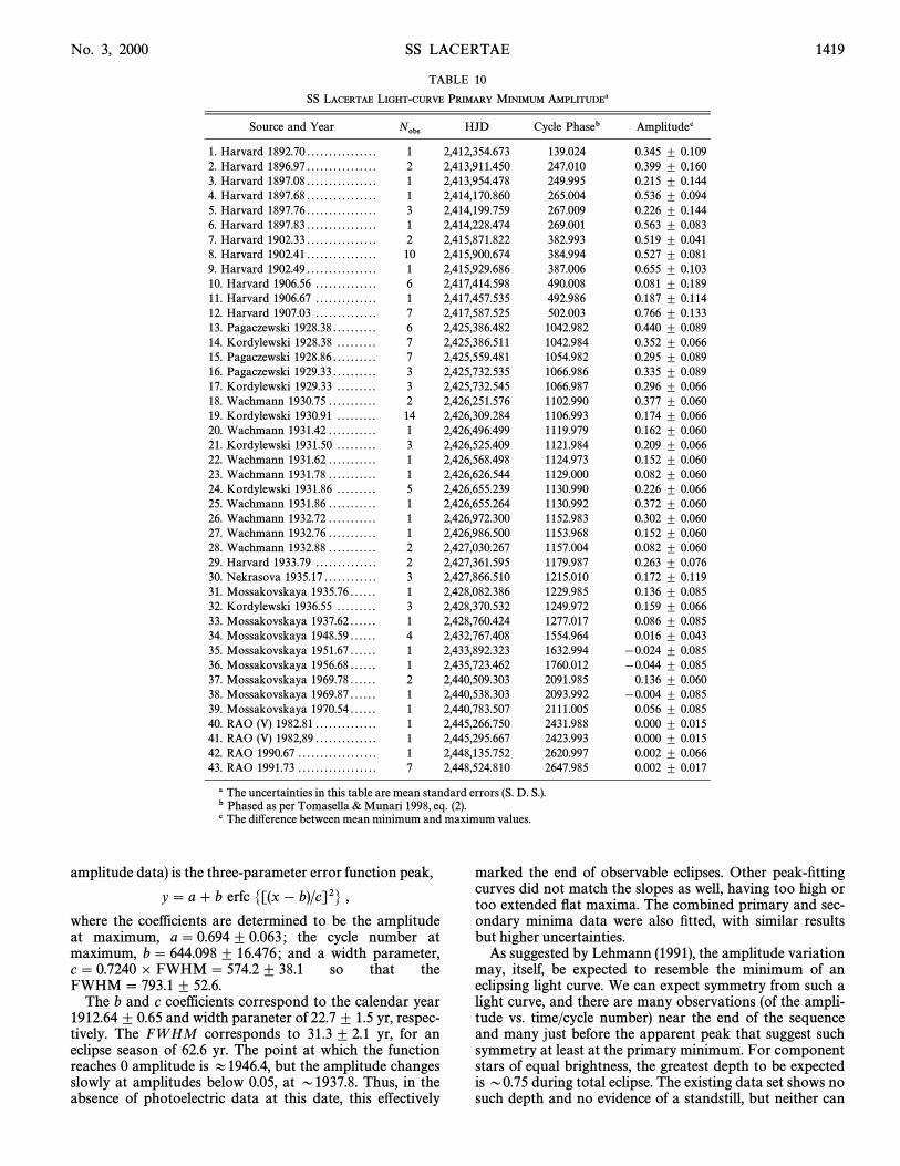
TABLE 10

SS LACERTAE LIGHT-CURVE PRIMARY MINIMUM AMPLITUDEa

Source and Year Nobs HJD Cycle Phaseb Amplitudec

1. Harvard 1892.70 . . . . . . . . . . . . . . . . 1 2,412,354.673 139.024 0.345 ^ 0.1092. Harvard 1896.97 . . . . . . . . . . . . . . . . 2 2,413,911.450 247.010 0.399 ^ 0.1603. Harvard 1897.08 . . . . . . . . . . . . . . . . 1 2,413,954.478 249.995 0.215 ^ 0.1444. Harvard 1897.68 . . . . . . . . . . . . . . . . 1 2,414,170.860 265.004 0.536 ^ 0.0945. Harvard 1897.76 . . . . . . . . . . . . . . . . 3 2,414,199.759 267.009 0.226 ^ 0.1446. Harvard 1897.83 . . . . . . . . . . . . . . . . 1 2,414,228.474 269.001 0.563 ^ 0.0837. Harvard 1902.33 . . . . . . . . . . . . . . . . 2 2,415,871.822 382.993 0.519 ^ 0.0418. Harvard 1902.41 . . . . . . . . . . . . . . . . 10 2,415,900.674 384.994 0.527 ^ 0.0819. Harvard 1902.49 . . . . . . . . . . . . . . . . 1 2,415,929.686 387.006 0.655 ^ 0.10310. Harvard 1906.56 . . . . . . . . . . . . . . 6 2,417,414.598 490.008 0.081 ^ 0.18911. Harvard 1906.67 . . . . . . . . . . . . . . 1 2,417,457.535 492.986 0.187 ^ 0.11412. Harvard 1907.03 . . . . . . . . . . . . . . 7 2,417,587.525 502.003 0.766 ^ 0.13313. Pagaczewski 1928.38 . . . . . . . . . . 6 2,425,386.482 1042.982 0.440 ^ 0.08914. Kordylewski 1928.38 . . . . . . . . . 7 2,425,386.511 1042.984 0.352 ^ 0.06615. Pagaczewski 1928.86 . . . . . . . . . . 7 2,425,559.481 1054.982 0.295 ^ 0.08916. Pagaczewski 1929.33 . . . . . . . . . . 3 2,425,732.535 1066.986 0.335 ^ 0.08917. Kordylewski 1929.33 . . . . . . . . . 3 2,425,732.545 1066.987 0.296 ^ 0.06618. Wachmann 1930.75 . . . . . . . . . . . 2 2,426,251.576 1102.990 0.377 ^ 0.06019. Kordylewski 1930.91 . . . . . . . . . 14 2,426,309.284 1106.993 0.174 ^ 0.06620. Wachmann 1931.42 . . . . . . . . . . . 1 2,426,496.499 1119.979 0.162 ^ 0.06021. Kordylewski 1931.50 . . . . . . . . . 3 2,426,525.409 1121.984 0.209 ^ 0.06622. Wachmann 1931.62 . . . . . . . . . . . 1 2,426,568.498 1124.973 0.152 ^ 0.06023. Wachmann 1931.78 . . . . . . . . . . . 1 2,426,626.544 1129.000 0.082 ^ 0.06024. Kordylewski 1931.86 . . . . . . . . . 5 2,426,655.239 1130.990 0.226 ^ 0.06625. Wachmann 1931.86 . . . . . . . . . . . 1 2,426,655.264 1130.992 0.372 ^ 0.06026. Wachmann 1932.72 . . . . . . . . . . . 1 2,426,972.300 1152.983 0.302 ^ 0.06027. Wachmann 1932.76 . . . . . . . . . . . 1 2,426,986.500 1153.968 0.152 ^ 0.06028. Wachmann 1932.88 . . . . . . . . . . . 2 2,427,030.267 1157.004 0.082 ^ 0.06029. Harvard 1933.79 . . . . . . . . . . . . . . 2 2,427,361.595 1179.987 0.263 ^ 0.07630. Nekrasova 1935.17 . . . . . . . . . . . . 3 2,427,866.510 1215.010 0.172 ^ 0.11931. Mossakovskaya 1935.76 . . . . . . 1 2,428,082.386 1229.985 0.136 ^ 0.08532. Kordylewski 1936.55 . . . . . . . . . 3 2,428,370.532 1249.972 0.159 ^ 0.06633. Mossakovskaya 1937.62 . . . . . . 1 2,428,760.424 1277.017 0.086 ^ 0.08534. Mossakovskaya 1948.59 . . . . . . 4 2,432,767.408 1554.964 0.016 ^ 0.04335. Mossakovskaya 1951.67 . . . . . . 1 2,433,892.323 1632.994 [0.024 ^ 0.08536. Mossakovskaya 1956.68 . . . . . . 1 2,435,723.462 1760.012 [0.044 ^ 0.08537. Mossakovskaya 1969.78 . . . . . . 2 2,440,509.303 2091.985 0.136 ^ 0.06038. Mossakovskaya 1969.87 . . . . . . 1 2,440,538.303 2093.992 [0.004 ^ 0.08539. Mossakovskaya 1970.54 . . . . . . 1 2,440,783.507 2111.005 0.056 ^ 0.08540. RAO (V) 1982.81 . . . . . . . . . . . . . . 1 2,445,266.750 2431.988 0.000 ^ 0.01541. RAO (V) 1982,89 . . . . . . . . . . . . . . 1 2,445,295.667 2423.993 0.000 ^ 0.01542. RAO 1990.67 . . . . . . . . . . . . . . . . . . 1 2,448,135.752 2620.997 0.002 ^ 0.06643. RAO 1991.73 . . . . . . . . . . . . . . . . . . 7 2,448,524.810 2647.985 0.002 ^ 0.017

a The uncertainties in this table are mean standard errors (S. D. S.).b Phased as per Tomasella & Munari 1998, eq. (2).c The di†erence between mean minimum and maximum values.

amplitude data) is the three-parameter error function peak,

y \ a ] b erfc M[(x [ b)/c]2N ,

where the coefficients are determined to be the amplitudeat maximum, a \ 0.694^ 0.063 ; the cycle number atmaximum, b \ 644.098^ 16.476 ; and a width parameter,c\ 0.7240] FWHM\ 574.2^ 38.1 so that theFWHM\ 793.1^ 52.6.

The b and c coefficients correspond to the calendar year1912.64^ 0.65 and width paraneter of 22.7 ^ 1.5 yr, respec-tively. The FW HM corresponds to 31.3 ^ 2.1 yr, for aneclipse season of 62.6 yr. The point at which the functionreaches 0 amplitude is B1946.4, but the amplitude changesslowly at amplitudes below 0.05, at D1937.8. Thus, in theabsence of photoelectric data at this date, this e†ectively

marked the end of observable eclipses. Other peak-Ðttingcurves did not match the slopes as well, having too high ortoo extended Ñat maxima. The combined primary and sec-ondary minima data were also Ðtted, with similar resultsbut higher uncertainties.

As suggested by Lehmann (1991), the amplitude variationmay, itself, be expected to resemble the minimum of aneclipsing light curve. We can expect symmetry from such alight curve, and there are many observations (of the ampli-tude vs. time/cycle number) near the end of the sequenceand many just before the apparent peak that suggest suchsymmetry at least at the primary minimum. For componentstars of equal brightness, the greatest depth to be expectedis D0.75 during total eclipse. The existing data set shows nosuch depth and no evidence of a standstill, but neither can


TABLE 11

SS LACERTAE LIGHT-CURVE SECONDARY MINIMUM AMPLITUDEa

Source Year Nobs HJD Cycle Phase Amplitudeb

1. Harvard 1893.59 . . . . . . . . . . . . . . . . 1 2,412,679.733 161.572 0.618 ^ 0.1272. Harvard 1897.30 . . . . . . . . . . . . . . . . 1 2,414,034.851 255.570 0.407 ^ 0.1073. Harvard 1897.38 . . . . . . . . . . . . . . . . 2 2,414,063.808 257.579 0.402 ^ 0.1224. Harvard 1897.78 . . . . . . . . . . . . . . . . 4 2,414,207.696 267.560 0.415 ^ 0.1755. Harvard 1897.86 . . . . . . . . . . . . . . . . 1 2,414,236.678 269.570 0.592 ^ 0.2206. Harvard 1897.94 . . . . . . . . . . . . . . . . 1 2,414,265.454 271.566 0.312 ^ 0.0907. Harvard 1899.63 . . . . . . . . . . . . . . . . 1 2,414,885.586 314.582 0.622 ^ 0.2428. Harvard 1900.03 . . . . . . . . . . . . . . . . 3 2,415,029.794 324.585 0.388 ^ 0.1349. Harvard 1902.67 . . . . . . . . . . . . . . . . 2 2,415,995.534 391.574 0.411 ^ 0.10810. Mossakovskaya 1902.75 . . . . . . 1 2,416,024.357 393.573 0.596 ^ 0.06511. Harvard 1906.66 . . . . . . . . . . . . . . 1 2,417,451.546 492.571 0.649 ^ 0.10612. Harvard 1908.36 . . . . . . . . . . . . . . 1 2,418,071.711 535.589 0.335 ^ 0.15513. Harvard 1923.55 . . . . . . . . . . . . . . 1 2,423,621.654 920.564 0.351 ^ 0.13414. Nekrasova 1926.27 . . . . . . . . . . . . 1 2,424,616.350 989.562 0.405 ^ 0.12015. Pagaczewski 1928.45 . . . . . . . . . . 1 2,425,409.425 1044.574 0.155 ^ 0.08916. Harvard 1928.76 . . . . . . . . . . . . . . 1 2,425,524.647 1052.566 0.209 ^ 0.11917. Wachmann 1931.48 . . . . . . . . . . . 1 2,426,519.494 1121.574 0.152 ^ 0.05918. Wachmann 1931.84 . . . . . . . . . . . 1 2,426,649.352 1130.582 0.032 ^ 0.05919. Wachmann 1931.96 . . . . . . . . . . . 1 2,426,692.444 1133.571 0.302 ^ 0.05920. Kordylewski 1933.66 . . . . . . . . . 2 2,427,312.399 1176.574 0.192 ^ 0.06521. Kordylewski 1935.67 . . . . . . . . . 1 2,428,047.458 1227.562 0.172 ^ 0.06522. Kordylewski 1936.97 . . . . . . . . . 4 2,428,523.262 1260.567 0.302 ^ 0.06523. Kordylewski 1937.05 . . . . . . . . . 1 2,428,552.232 1262.576 0.132 ^ 0.06524. Harvard 1937.76 . . . . . . . . . . . . . . 1 2,428,811.634 1280.570 0.308 ^ 0.13025. Mossakovskaya 1969.77 . . . . . . 1 2,440,503.418 2091.577 0.136 ^ 0.06526. Mossakovskaya 1971.75 . . . . . . 1 2,441,224.514 2141.596 0.066 ^ 0.06527. Mossakovskaya 1974.70 . . . . . . 1 2,442,305.302 2216.565 [0.014 ^ 0.065

a The uncertainties in this table are mean standard errors (S. D. S.).b The di†erence between mean minimum and maximum values.

be ruled out because of gaps in the data. ConÐrmed obser-vation of any minima outside the dates of extrapolated zerowould be interesting, since they are unexpected, and sowould data in the gap when the amplitude should have beenat maximum.

The Ischenko estimates of the Tashkent plates referred toin ° 2.1 are presented on time and phase axes in Figure 8.They support rather dramatically the evidence for an e†ec-tive absence of eclipses in about D1937 and further ques-tion the credibility of the Tashpulatov (1965) light curve.Since the data set of Nekrasova (1938), though sparse, and

the extensive compilations of Mossakovskaya (1993) pointto the same conclusion, this essentially clinches the matter.The overall results conÐrm the conclusion of Lehmann(1991) of an apparent decrease in amplitude in the 1920sand 1930s, and we conÐrm that the apparent maximum inthe amplitude seems to have been reached in the early yearsof this century, in about 1911.

The light-curve results are sufficiently uncertain thatvariations in certain other parameters, such as the radius ofone of the stars, cannot be ruled out. The formal solutionsindicate a larger di†erence in monochromatic luminosity

FIG. 8.ÈLight curve of SS Lacertae based on more recent estimates from Tashkent plates taken between 1937 and 1940 by I. M. Ischenko and byM. Zakirov (1998, private communication). The magnitude estimates were averaged and the di†erences between the individual values taken to produce theplots. L eft, The time-sequence behavior of the data ; right, the phased data, produced with the elements of Tomasella & Munari (1998). Together with Fig. 7,these plots support the suggestion of Mossakovskaya (1993) that eclipses ceased between 1937 and 1940.


(2]) between the components than does the present spec-tral study, which indicates the more massive star (star 2) tobe slightly more luminous (Tomasella & Munari 1998). It ismore likely, however, that evidence of variation from di†er-ing parameters for di†erent light-curve sets arises fromlight-curve anomalies introduced by the apparent variabledepth of eclipses.

We have noted that the Dugan & Wright (1935) meanlight curve is a composite of variable light curves, especiallyin the area of the secondary minimum. The main e†ect ofthis variation seems to be a larger scatter in the depth of thesecondary minimum than is seen in the primary minimum.The scatter in the Kordylewski data, which are quitenumerous and consistent in the maximum, with p1 \^0.065, is larger in the minima, especially the secondaryminimum, even though the mean depth does not exceedD0.3 mag. However, the explanation may lie in a remark byHo†meister (1921) that he, at least, found it difficult to esti-mate the brightness of SS Lac because of its small lightvariation and the rich numbers of stars of nearly equalbrightness in the star cluster.

The minima from the 1930s show amplitudes D0.4 mag,in agreement with the amplitude in the HCO data fromD1900. The detailed plots of the cycle-to-cycle amplitudesreveal apparent variation in both minima. Figure 5 showsthat the variation of the inclination over the data sets causesa cycle-to-cycle change in the amplitude of the system; theaveraging of data sets over several years results in anaverage minimum depth that is not greatly di†erent in thetwo principal sets we analyze here.

To categorize the behavior of the system, a series ofexperiments was performed with the Binary Maker 2.0 soft-ware of Bradstreet (1993), which, although unsuited to fullyexplore eccentric orbit cases, provides an indication of howthis is possible. The experiments demonstrate that totaleclipses for the DW35 Ðtting model occur for all inclina-tions greater than while the depths of the eclipsesD88¡.1,decrease slowly for decreases in i to about TheD87¡.5.decrease is more rapid thereafter until the cessation ofeclipses altogether at i\ D 82¡. The BM2.0 experimentscoupled with the parabolic Ðt of the individual cycle ampli-tudes suggest that the total range of inclination variationover a 26 yr interval is about 8¡. If the motion were purelysecular and uniform, the period of revolution of the orbitalplane would be D1200 yr, in agreement with that found byTomasella & Munari (1998), 1275^ 90 yr. A slight reÐne-ment is found by making use of the derived values of theinclination for the modeled data sets (see Fig. 9). Since it is

FIG. 9.ÈDerived inclinations from the Ðnal models of all analyzed datasets, and the limit from eclipse cessation simulations. The 90¡ inclinationplacement at the year 1912 is derived from the Harvard plates light curveamplitude study begun by S. J. S. ; that at 1997 is due to the iteratedsolution for the TM98 data set ; that at 82¡ is the epoch of eclipse cessation.

iterated with the DW35 set, the TM98 point is neither inde-pendent nor a mere extrapolation, but lies along a line satis-Ðed, within errors, by the other points.

We noted in ° 3.2 that an optimum value for wasi\ 76¡.5obtained. If this is accurate, we have over the 1998È1912span of years a change of for a variation of13¡.5 B0¡.157yr~1, for a period of D2300 yr or an interval betweeneclipses of length D1150 yr (if the orbital motion of the SSLac system permits eclipses to be seen at both nodes).

Within errors, Tables 6, 7, and 8 suggest no discernibleapsidal motion to be present in the system, in agreementwith statements by Dugan & Wright (1935), Dugan &Wright (1937), and Shapley & Swope (1938).

Regrettably, the data in hand for individual observationsof the minima in the early HCO data are too sparse andnoisy for short-interval light-curve precision modeling atpresent, which could conÐrm the amplitude and parametervariation predictions over short intervals. It would be ofgreat value to have available the full set of Ho†meisterÏs(1921) estimates, which cover only a narrow range of dates,the full set of Harvard estimates, and the full archival set ofSonneberg data. According to T. Lehmann (1993, privatecommunication), e†orts were underway, at one point, tomeasure these plates. S. J. S. plans further work in this areato improve our knowledge of the behavior of this system,especially around the predicted date of maximum eclipse,1912.

In any case, the system has certainly not been disruptedas had sometimes been conjectured. The strongest evidencefor this scenario was a CCF analysis (Schller & Milone1996) in which the hydrogen lines were excluded (see ° 2.2).A reexamination of the intensiÐed Reticon spectral regis-tration shows broad and noisy cores in the Balmer linesand, although sometimes suggestive, no Ðrm evidence ofsplitting. Apparently, the S/N in these spectra was insuffi-ciently high to reveal the SB2 character of the system.

Regarding the third component, it is interesting to notethat the mean radial velocity from 12 exposures found byS. J. S., [ 24.9^ 4.8 km s~1, is in agreement with the thirdcomponent radial velocity seen at quadratures by Toma-sella & Munari 1998 ([22.3^ 3.0) and that these values arenot signiÐcantly di†erent from the Tomasella & Munarimean radial velocity determination ([21.2^ 0.3), fromthat derived here ([19.9^ 0.8), or from the mean velocityof three giants in NGC 7209 measured by J.-P. Mermilliod(1995, private communication to S. J. S. ; [19.1^ 0.2).

We note that the derived distance for the system (Table9), 898 ^ 95 pc, is in approximate(V0[ M

V) \ 9.77^ 0.23,

agreement with that found for SS Lac in the Vilnius photo-metry study of NGC 7209 by et al. (1997),Vansevic— ius1040 ^ 10 pc, computed on the basis of equal luminosity forthe components. This value is also close to their value forthe cluster distance, 1026 ^ 15, corresponding to a cor-rected distance modulus of 10.06^ 0.06. Their derived Vmagnitude of the SS Lac system (their star 1828) is 10.07.Our result is not, however, consistent with that of &Pen8 aPeniche (1994), who Ðnd a distance for SS Lac (their star 16)of only 634 pc and place it in the closer of what they argueare two superposed clusters. Because et al.Vansevic— ius(1997) closely scrutinized the stars they included for mem-bership, we accept their determination for the cluster dis-tance (if not their distance for SS Lac, since our solutionssuggest disparate luminosities) and thus the unitary qualityof the cluster.


Therefore, on the grounds of proximity on the sky,proper motion, radial velocity, photometry, and derivedproperties, the binary is conÐrmed as belonging to NGC7209. Moreover, on the basis of its apparent connection tothe binary, and radial velocity agreement with it, the thirdcomponent seen at quadratures by Tomasella & Munari(1998) in the spectra is a probable cluster member, as well asthe likely source of the binaryÏs nodal motion.

The studies of (1974, 1975) of the behavior ofSo� derhjelmthe triple systems b Per, AY Mus, and j Tau suggest thatnodal variation may be accompanied by apsidal motionand characterized by variable separation and widths of theeclipses. Thus far, at least, no certain evidence is seen forthese e†ects in SS Lac.

An upper limit to the angular separation of the thirdcomponent from the close binary, either through HubbleSpace Telescope or ground-based adaptive optics, would beuseful. It would also be useful to obtain high-resolutionradial velocities, from which the period of the mutual orbitof the close binary and the third component could be found.The results of current modeling suggest that the contribu-tion from a third light source could be hidden in the noise inthe photographic light curves and in almost all of the Kdata set modeling. In the W36 model 3, exceeds its error,l3but only marginally. In the K model 3 of Table 8, isl3signiÐcantly greater than its uncertainty, but in that model,

The noise level sets the limit in thel3B 27%. l3[ 2%DW35 data set modeling. Given the relative dimness of thethird starÏs contribution to B and its weak detection in theBalmer a, b, and c lines, one would suppose it to be both lessluminous and more red than the other components. A studyin the infrared is underway at the RAO to check this possi-bility.

The curious circumstance that the components essen-tially agree in mass and in temperature and yet di†er signiÐ-

cantly in radius is enigmatic, if the solutions presented hereare to be believed. Unfortunately, there seems little chanceto improve on the solutions until more archival data cometo light or the system begins to eclipse again. It is instruc-tive, however, that the initial Russell solution of Dugan &Wright as well as each of the photometric sets we analyzedin the present work yields disparate values for the eclipsingcomponentsÏ luminosities and sizes. The location of the SSLac components on the blue side of the CMD, and justbelow the cluster turn-o†, continues to make this systemimportant as a check on stellar evolution models ; perhapsastronomers of the fourth (or Ðfth !) millenium may also Ðndit so.

We are grateful for several grants that have supportedthis work : Support to E. F. M. has come from the Uni-versity of Calgary Research Grants Committee and fromNSERC of Canada ; research support to S. J. S. has beenprovided by a Northwest Area Foundation Grant of theResearch Corporation, the NASA SDSU JOVE program, aNASA grant administered by the American AstronomicalSociety, NSF grant OSR 94-52894 and by the SouthDakota Future Fund. Steven Griffin, James van Leeuwen,Jason McVean, and Perry Radau helped in the acquisitionof the photoelectric data summarized in Table 1. David Fryand Eric Leblanc provided important copies of critical ref-erences from DAOÏs library. A special word of gratitudeshould be voiced for the careful work of the Cracow obser-vers, and to Rosa Szafraniecz, who enabled these valuabledata to come to light. See Milone et al. (1980) for theircontributions to the study of another interesting variable,RW Com. This research has made use of the SIMBADdatabase, operated at CDS, Strasbourg, France.

REFERENCES

Artiukhina, N. M. 1961, Trudy. Astron. Inst. Sternberg, 30, 196Bradstreet, D. H. 1993, Binary Maker 2.0 User Manual (Norristown, PA:

Contact Software)Dugan, R. S., & Wright, F. W. 1935, AJ, 44, 150ÈÈÈ. 1937, AJ, 46, 148Etzel, P. B., & Vogelnau, N. H. 1996, IAU Circ. 6344Etzel, P. B., Vogelnau, N. H., & Nguyen, Q. T. 1996, IAU Circ. 6429Harries, T. J., Hilditch, R. W., & Hill, G. 1998, MNRAS, 295, 386Hill, G. 1982, Publ. Dom. Astrophys. Obs. Victoria, 16, 59Hill, G., Fisher, W. A., & Poeckert, R. 1982, Publ. Dom. Astrophys. Obs.

Victoria, 16, 43Hoag, A. A., Johnson, H. L., Iriarte, B., Mitchell, R. I., Hallam, K. L., &

Sharpless, S. 1961, Publ. US Naval Obs., 17, 347Ho†meister, C. 1921, Astron. Nachr., 214, 7Kallrath, J. 1993, in Light Curve Modeling of Eclipsing Binary Stars, ed.

E. F. Milone (New York : Springer), 39Kallrath, J., & Milone, E. F. 1999, Eclipsing Binary Stars : Modeling and

Analysis (New York : Springer)Kallrath, J., Milone, E. F., Terrell, D., & Young, A. T. 1998, ApJ, 508, 308Kordylewski, K., Pagaczewski, J., & Szafraniec, R. 1961, Acta Astron.

Suppl., 4, 487Kurucz, R. L. 1993, in Light Curve Modeling of Eclipsing Binary Stars, ed.

E. F. Milone (New York : Springer), 93Lacy, C. 1992, AJ, 104, 801Lavdovska, V. V. 1962, Izv. Pulkovo Obs., 24, 69Lehmann, T. 1991, Inf. Bull. Variable Stars 3610Milone, E. F., Chia, T. T., Castle, K. G., Robb, R. M., & Merrill, J. E. 1980,

ApJS, 43, 339Milone, E. F., & Robb, R. M. 1983, PASP, 95, 666Milone, E. F., Robb, R. M., Babott, F. M., & Hansen, C. H. 1982, Appl.

Opt., 21, 2992Milone, E. F., & Schiller, S. J. 1998, BAAS, 30, 1155Milone, E. F., Stagg, C. R., & Kurucz, R. L. 1992a, ApJS, 79, 123

Milone, E. F., Stagg, C. R., & Schiller, S. J. 1992b, in Evolutionary Pro-cesses in Interacting Binary Stars, ed. Y. Kondo, R. F. Sistero, & R. S.Polidan (Dordrecht : Kluwer), 479

Mossakovskaya, L. V. 1993, Astron. Lett., 19, 35Nekrasova, S. 1938, Perem. Zvezdy, 5, 182

J. H., & Peniche, R. 1994, Rev. Mexicana Astron. AstroÐs., 28, 139Pen8 a,Pickering, E. C. 1907, Harvard Circ. 130Platais, I. 1991, A&AS, 87, 577Popper, D. M. 1980, ARA&A, 18, 115Sandberg Lacy, C. H., Helt, B. E., & Vaz, L. P. R. 1999, AJ, 117, 541Schaefer, B. E. 1981, PASP, 93, 225Schaefer, B. E., & Fried, R. E. 1991, AJ, 101, 208Schiller, S. J., & Milone, E. F. 1987, AJ, 93, 1471Schiller, S. J., Bridges, D., & Clifton, T. 1996, in ASP Conf. Proc. 90, The

Origins, Evolution, and Destinies of Binary Stars in Clusters, ed. E. F.Milone & J.-C. Mermilliod (San Francisco : ASP), 141

ÈÈÈ. 1996, in ASP Conf. Proc. 90, The Origins, Evolution, and Destiniesof Binary Stars in Clusters, ed. E. F. Milone & J.-C. Mermilliod (SanFrancisco : ASP), 120

Schiller, S. J., Milone, E. F., Zakirov, M. M., & Azimov, A. A. 1991, BAAS,23, 879

Shapley, H., & Swope, H. H. 1938, Hvar Obs. Bull., 909, 5S. 1974, Inf. Bull. Variable Stars 855So� derhjelm,S. 1975, A&A, 42, 229So� derhjelm,

Stagg, C. R., & Milone, E. F. 1993, Light Curve Modeling of EclipsingBinary Stars, ed. E. F. Milone (New York : Springer), 75

Stefanik, R. P., Torres, G., Caruso, J. R., & Davis, R. J. 1996, IAU Circ.6433

Svolopoulos, S. 1961, ApJ, 134, 612Tashpulatov, N. 1965, Perem. Zvezdy, 15, 424Tomasella, L., & Munari, U. 1998, A&A, 335, 561Twarog, B. A., Ashman, K. M., & Anthony-Twarog, B. J. 1997, AJ, 114,

2556


van Schewick, H. 1966, Astron. Inst. Univ. Bonn, 70, 1Vero� †.V., Platais, I., Paupers, O., & 1997, MNRAS, 285,Vansevic— ius, A1 bolins— , E1 .

871Wachmann, A. A. 1935, Astron. Nachr., 255, 340Wachmann, A. A. 1936, Astron. Nachr., 258, 361

Wilson, R. E. 1963, General Catalog of Radial Velocties (Carnegie Publ.601) (Washington : Carnegie Inst.)

ÈÈÈ. 1992, Documentation of Eclipsing Binary Star Model (Gainesville :Univ. Florida)

Zakirov, M. M., & Azimov, A. A. 1990, Inf. Bull. Variable Stars 3487

the astronomical journal,119:1405 …kallrath/files/sslac2000.pdf · · 2007-02-25the...

Documents