the arithmetic of elliptic curves - armstrong · the arithmetic of elliptic curves sungkon chang...
TRANSCRIPT
The Arithmetic of Elliptic Curves
Sungkon Chang
The Anne and Sigmund HudsonMathematics and ComputingLuncheon Colloquium Series
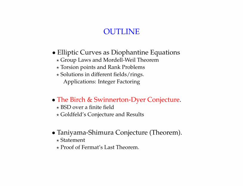
OUTLINE
• Elliptic Curves as Diophantine Equations? Group Laws and Mordell-Weil Theorem? Torsion points and Rank Problems? Solutions in different fields/rings.
Applications: Integer Factoring
• The Birch & Swinnerton-Dyer Conjecture.? BSD over a finite field? Goldfeld’s Conjecture and Results
• Taniyama-Shimura Conjecture (Theorem).? Statement? Proof of Fermat’s Last Theorem.
Elliptic Curves
An elliptic curve is an equation E : y2 = x3 +Ax+B(where x3 +Ax+B = 0 has distinct roots).
Sets of solutions: E(Z), E(Q), E(R), E(C), E(Z/nZ), . . . .
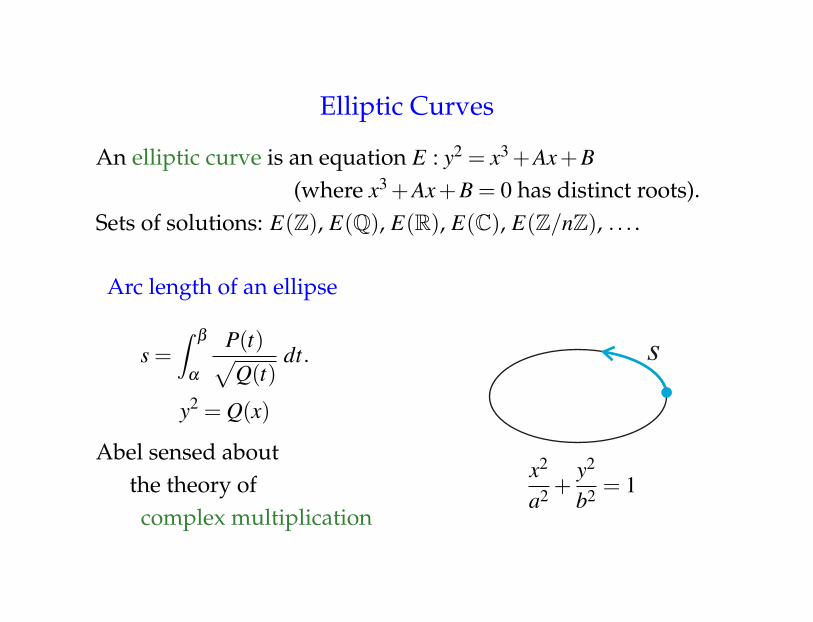
Elliptic Curves
An elliptic curve is an equation E : y2 = x3 +Ax+B(where x3 +Ax+B = 0 has distinct roots).
Sets of solutions: E(Z), E(Q), E(R), E(C), E(Z/nZ), . . . .
Arc length of an ellipse
s =∫
β
α
P(t)√Q(t)
dt.
y2 = Q(x)
Abel sensed aboutthe theory ofcomplex multiplication
x2
a2 +y2
b2 = 1
Elliptic Curves
An elliptic curve is an equation E : y2 = x3 +Ax+B(where x3 +Ax+B = 0 has distinct roots).
Sets of solutions: E(Z), E(Q), E(R), E(C), E(Z/nZ), . . . .
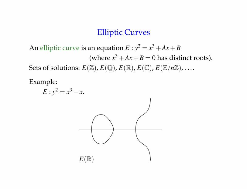
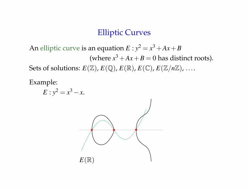
Example:E : y2 = x3− x.
E(R)
Elliptic Curves
An elliptic curve is an equation E : y2 = x3 +Ax+B(where x3 +Ax+B = 0 has distinct roots).
Sets of solutions: E(Z), E(Q), E(R), E(C), E(Z/nZ), . . . .
Example:E : y2 = x3− x.
E(R)
Elliptic Curves
An elliptic curve is an equation E : y2 = x3 +Ax+B(where x3 +Ax+B = 0 has distinct roots).
Sets of solutions: E(Z), E(Q), E(R), E(C), E(Z/nZ), . . . .
E(C) is a Riemann surfaceof genus 1.

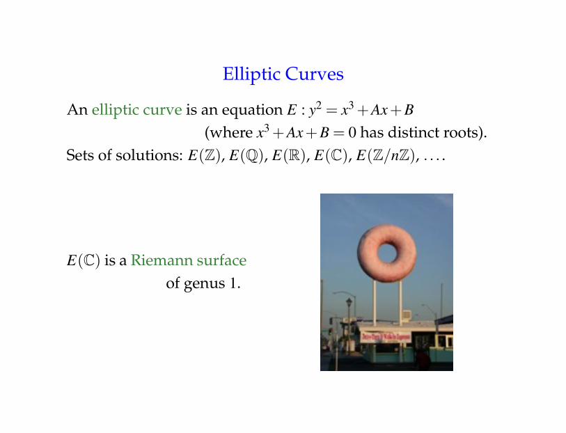
Elliptic Curves
An elliptic curve is an equation E : y2 = x3 +Ax+B(where x3 +Ax+B = 0 has distinct roots).
Sets of solutions: E(Z), E(Q), E(R), E(C), E(Z/nZ), . . . .
E(C)

Elliptic Curves
An elliptic curve is an equation E : y2 = x3 +Ax+B(where x3 +Ax+B = 0 has distinct roots).
Sets of solutions: E(Z), E(Q), E(R), E(C), E(Z/nZ), . . . .
E(R)

Elliptic Curves
An elliptic curve is an equation E : y2 = x3 +Ax+B(where x3 +Ax+B = 0 has distinct roots).
Sets of solutions: E(Z), E(Q), E(R), E(C), E(Z/nZ), . . . .
E(R)
Elliptic Curves
An elliptic curve is an equation E : y2 = x3 +Ax+B
(where x3 +Ax+B = 0 has distinct roots).Sets of solutions: E(Z), E(Q), E(R), E(C), E(Z/nZ), . . . .
Diophantine Equations in two variables: e.g., X : x2 + y2 = 1
Q rat’l // X(Q)
t //
(1− t2
1+ t2 ,2t
1+ t2
)

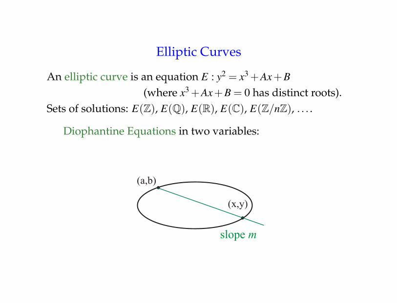
Elliptic Curves
An elliptic curve is an equation E : y2 = x3 +Ax+B(where x3 +Ax+B = 0 has distinct roots).
Sets of solutions: E(Z), E(Q), E(R), E(C), E(Z/nZ), . . . .
Diophantine Equations in two variables: e.g., X : x2 + y2 = 1
Elliptic Curves
An elliptic curve is an equation E : y2 = x3 +Ax+B(where x3 +Ax+B = 0 has distinct roots).
Sets of solutions: E(Z), E(Q), E(R), E(C), E(Z/nZ), . . . .
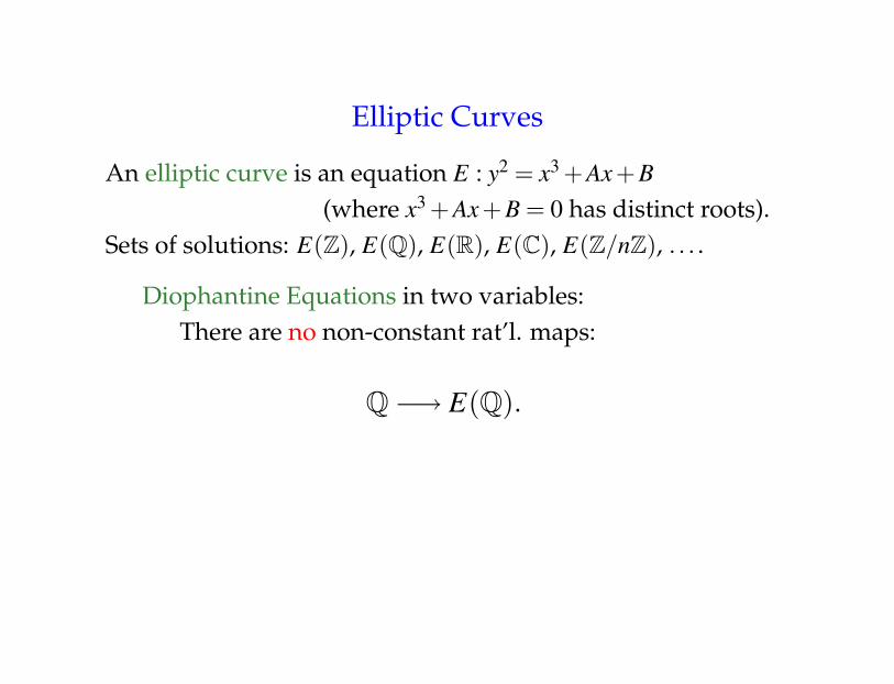
Diophantine Equations in two variables:
Elliptic Curves
An elliptic curve is an equation E : y2 = x3 +Ax+B(where x3 +Ax+B = 0 has distinct roots).
Sets of solutions: E(Z), E(Q), E(R), E(C), E(Z/nZ), . . . .
Diophantine Equations in two variables:There are no non-constant rat’l. maps:
Q−→ E(Q).

Elliptic Curves
An elliptic curve is an equation E : y2 = x3 +Ax+B(where x3 +Ax+B = 0 has distinct roots).
Sets of solutions: E(Z), E(Q), E(R), E(C), E(Z/nZ), . . . .
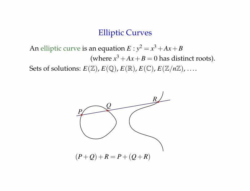
Elliptic Curves
An elliptic curve is an equation E : y2 = x3 +Ax+B(where x3 +Ax+B = 0 has distinct roots).
Sets of solutions: E(Z), E(Q), E(R), E(C), E(Z/nZ), . . . .
(P+Q)+R = P+(Q+R)
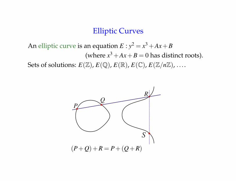
Elliptic Curves
An elliptic curve is an equation E : y2 = x3 +Ax+B(where x3 +Ax+B = 0 has distinct roots).
Sets of solutions: E(Z), E(Q), E(R), E(C), E(Z/nZ), . . . .
(P+Q)+R = P+(Q+R)
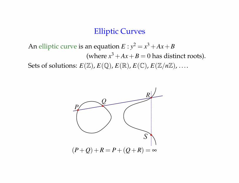
Elliptic Curves
An elliptic curve is an equation E : y2 = x3 +Ax+B(where x3 +Ax+B = 0 has distinct roots).
Sets of solutions: E(Z), E(Q), E(R), E(C), E(Z/nZ), . . . .
(P+Q)+R = P+(Q+R) = ∞

Elliptic Curves
An elliptic curve is an equation E : y2 = x3 +Ax+B(where x3 +Ax+B = 0 has distinct roots).
Sets of solutions: E(Z), E(Q), E(R), E(C), E(Z/nZ), . . . .
E(Q) = E(Q)∪{∞}
(P+Q)+R = P+(Q+R) = ∞

Elliptic Curves
An elliptic curve is an equation E : y2 = x3 +Ax+B(where x3 +Ax+B = 0 has distinct roots).
Sets of solutions: E(Z), E(Q), E(R), E(C), E(Z/nZ), . . . .
Group law:(a,b)+(c,d) :=(
−−b2 +2bd−d2 +a3−a2c−ac2 + c3
(a− c)2 ,
− 1(a− c)3 (−b3 +3b2d−3bd2 +ba3 +2bc3
+d3−2da3 +3da2c−dc3−3bac2)
)
Elliptic Curves
An elliptic curve is an equation E : y2 = x3 +Ax+B(where x3 +Ax+B = 0 has distinct roots).
Sets of solutions: E(Z), E(Q), E(R), E(C), E(Z/nZ), . . . .
Mordell-Weil Thm: There are points P1, . . . ,Pr in E(Q) s.t.
E(Q) = {m1P1 + · · ·+mrPr : mi are integers}.
Elliptic Curves
An elliptic curve is an equation E : y2 = x3 +Ax+B(where x3 +Ax+B = 0 has distinct roots).
Sets of solutions: E(Z), E(Q), E(R), E(C), E(Z/nZ), . . . .
Mordell-Weil Thm: There are points P1, . . . ,Pr in E(Q) s.t.
E(Q) = {m1P1 + · · ·+mrPr : mi are integers}.
example: E : y2 = x3 +17.? E(Q) contains P = (−1,4).

Elliptic Curves
An elliptic curve is an equation E : y2 = x3 +Ax+B(where x3 +Ax+B = 0 has distinct roots).
Sets of solutions: E(Z), E(Q), E(R), E(C), E(Z/nZ), . . . .
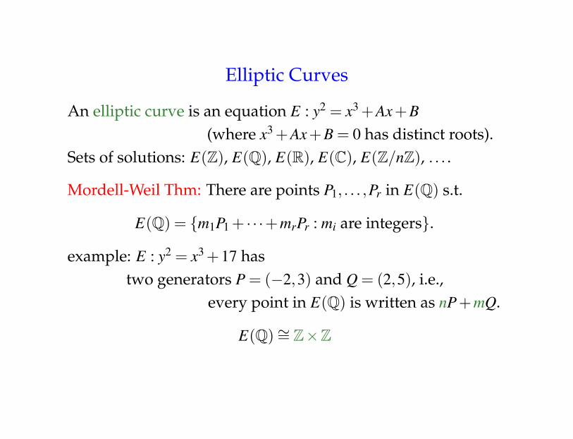
Mordell-Weil Thm: There are points P1, . . . ,Pr in E(Q) s.t.
E(Q) = {m1P1 + · · ·+mrPr : mi are integers}.
example: E : y2 = x3 +17.? E(Q) contains P = (−1,4).? E(Q) contains 6P =(3703710745675909854372790801
699522170992056989781928164 ,
26061553437018470170642497173368633399980118501299163096718454375010188444627517288
).
Elliptic Curves
An elliptic curve is an equation E : y2 = x3 +Ax+B(where x3 +Ax+B = 0 has distinct roots).
Sets of solutions: E(Z), E(Q), E(R), E(C), E(Z/nZ), . . . .
Mordell-Weil Thm: There are points P1, . . . ,Pr in E(Q) s.t.
E(Q) = {m1P1 + · · ·+mrPr : mi are integers}.
example: E : y2 = x3 +17 hastwo generators P = (−2,3) and Q = (2,5), i.e.,
every point in E(Q) is written as nP+mQ.
E(Q)∼= Z×Z

Elliptic Curves
An elliptic curve is an equation E : y2 = x3 +Ax+B(where x3 +Ax+B = 0 has distinct roots).
Sets of solutions: E(Z), E(Q), E(R), E(C), E(Z/nZ), . . . .
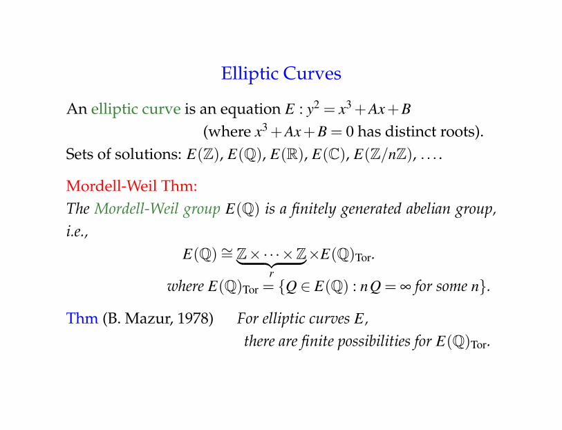
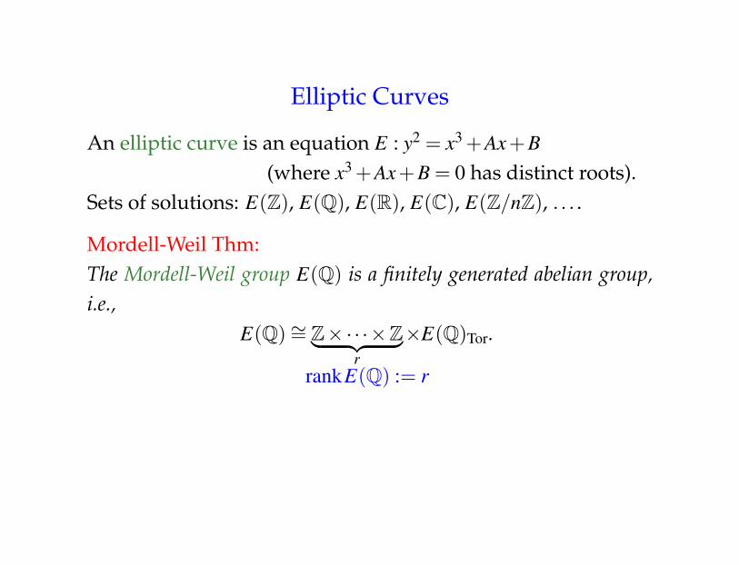
Mordell-Weil Thm:The Mordell-Weil group E(Q) is a finitely generated abelian group,i.e.,
E(Q)∼= Z×·· ·×Z︸ ︷︷ ︸r
×E(Q)Tor.
rankE(Q) := rwhere E(Q)Tor = {Q ∈ E(Q) : nQ = ∞ for some n}.
Elliptic Curves
An elliptic curve is an equation E : y2 = x3 +Ax+B(where x3 +Ax+B = 0 has distinct roots).
Sets of solutions: E(Z), E(Q), E(R), E(C), E(Z/nZ), . . . .
Mordell-Weil Thm:The Mordell-Weil group E(Q) is a finitely generated abelian group,i.e.,
E(Q)∼= Z×·· ·×Z︸ ︷︷ ︸r
×E(Q)Tor.
where E(Q)Tor = {Q ∈ E(Q) : nQ = ∞ for some n}.
Thm (B. Mazur, 1978) For elliptic curves E,there are finite possibilities for E(Q)Tor.
Elliptic Curves
An elliptic curve is an equation E : y2 = x3 +Ax+B(where x3 +Ax+B = 0 has distinct roots).
Sets of solutions: E(Z), E(Q), E(R), E(C), E(Z/nZ), . . . .
Mordell-Weil Thm:The Mordell-Weil group E(Q) is a finitely generated abelian group,i.e.,
E(Q)∼= Z×·· ·×Z︸ ︷︷ ︸r
×E(Q)Tor.
rankE(Q) := r

Elliptic Curves
An elliptic curve is an equation E : y2 = x3 +Ax+B(where x3 +Ax+B = 0 has distinct roots).
Sets of solutions: E(Z), E(Q), E(R), E(C), E(Z/nZ), . . . .Mordell-Weil Thm: E(Q)∼= Z×·· ·×Z×E(Q)Tor.
Open Questions• Find generators of E(Q).• Find an algorithm that computes rankE(Q).• Prove ∃ ∞ly many E’s with arbitrarily large rankE(Q).
Record: In 2006, N. Elkies found E for which rankE(Q)≥ 28.
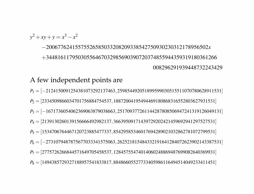
y2 + xy+ y = x3− x2
−20067762415575526585033208209338542750930230312178956502x
+34481611795030556467032985690390720374855944359319180361266
008296291939448732243429
A few independent points areP1 = [−2124150091254381073292137463,259854492051899599030515511070780628911531]
P2 = [2334509866034701756884754537,18872004195494469180868316552803627931531]
P3 = [−1671736054062369063879038663,251709377261144287808506947241319126049131]
P4 = [2139130260139156666492982137,36639509171439729202421459692941297527531]
P5 = [1534706764467120723885477337,85429585346017694289021032862781072799531]
P6 = [−2731079487875677033341575063,262521815484332191641284072623902143387531]
P7 = [2775726266844571649705458537,12845755474014060248869487699082640369931]
P8 = [1494385729327188957541833817,88486605527733405986116494514049233411451]
Modular Arithmetic
An elliptic curve is an equation E : y2 = x3 +Ax+Bwhere A,B are integers.
The set of residue classes Z/nZ := {0,1, . . . ,n−1}.
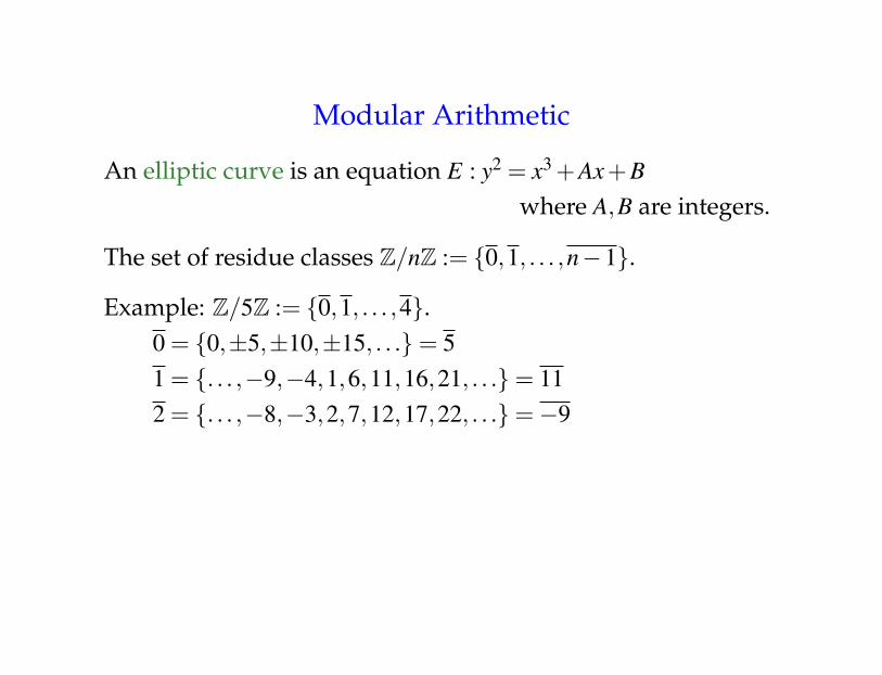
Modular Arithmetic
An elliptic curve is an equation E : y2 = x3 +Ax+Bwhere A,B are integers.
The set of residue classes Z/nZ := {0,1, . . . ,n−1}.
Example: Z/5Z := {0,1, . . . ,4}.0 = {0,±5,±10,±15, . . .}= 51 = {. . . ,−9,−4,1,6,11,16,21, . . .}= 112 = {. . . ,−8,−3,2,7,12,17,22, . . .}=−9

Modular Arithmetic
An elliptic curve is an equation E : y2 = x3 +Ax+Bwhere A,B are integers.
The set of residue classes Z/nZ := {0,1, . . . ,n−1}.
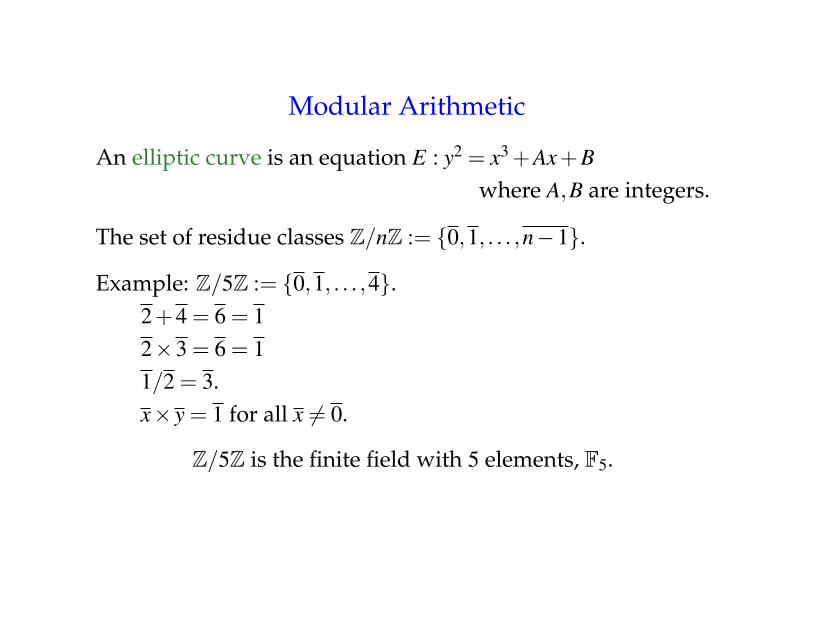
Example: Z/5Z := {0,1, . . . ,4}.2+4 = 6 = 12×3 = 6 = 11/2 = 3.x× y = 1 for all x 6= 0.
Modular Arithmetic
An elliptic curve is an equation E : y2 = x3 +Ax+Bwhere A,B are integers.
The set of residue classes Z/nZ := {0,1, . . . ,n−1}.
Example: Z/5Z := {0,1, . . . ,4}.2+4 = 6 = 12×3 = 6 = 11/2 = 3.x× y = 1 for all x 6= 0.
Z/5Z is the finite field with 5 elements, F5.
Modular Arithmetic
An elliptic curve is an equation E : y2 = x3 +Ax+Bwhere A,B are integers.
The set of residue classes Z/nZ := {0,1, . . . ,n−1}.
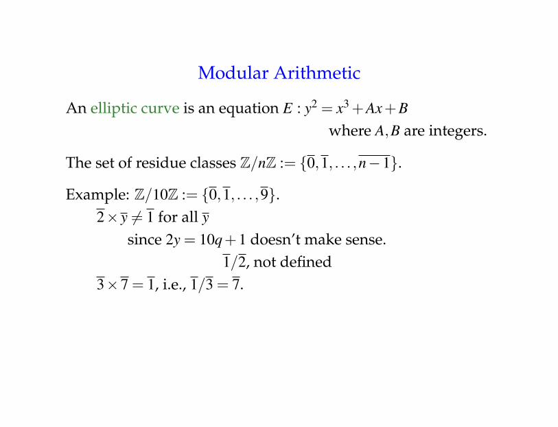
Example: Z/10Z := {0,1, . . . ,9}.2× y 6= 1 for all y
since 2y = 10q+1 doesn’t make sense.1/2, not defined
3×7 = 1, i.e., 1/3 = 7.
Modular Arithmetic
An elliptic curve is an equation E : y2 = x3 +Ax+Bwhere A,B are integers.
The set of residue classes Z/nZ := {0,1, . . . ,n−1}.
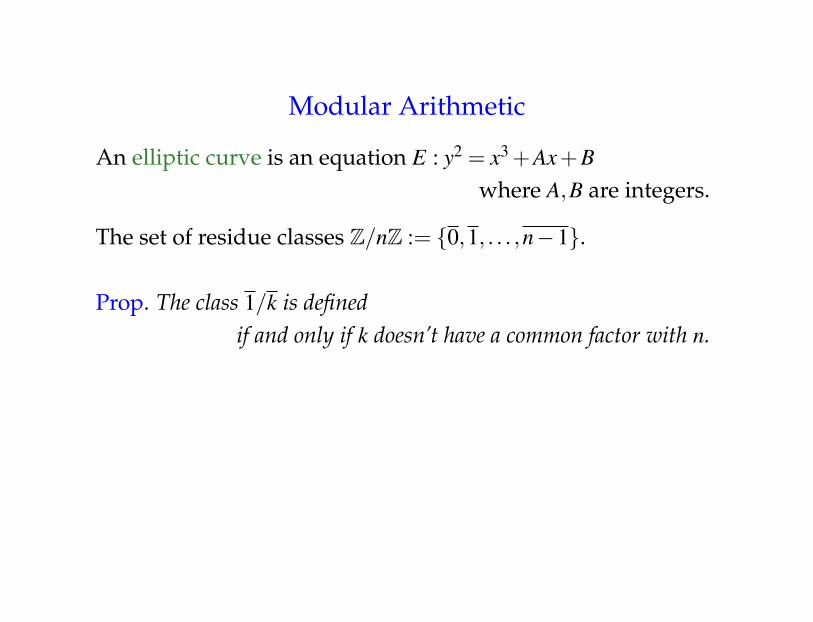
Prop. The class 1/k is definedif and only if k doesn’t have a common factor with n.
Modular Arithmetic
An elliptic curve is an equation E : y2 = x3 +Ax+Bwhere A,B are integers.
The set of residue classes Z/nZ := {0,1, . . . ,n−1}.
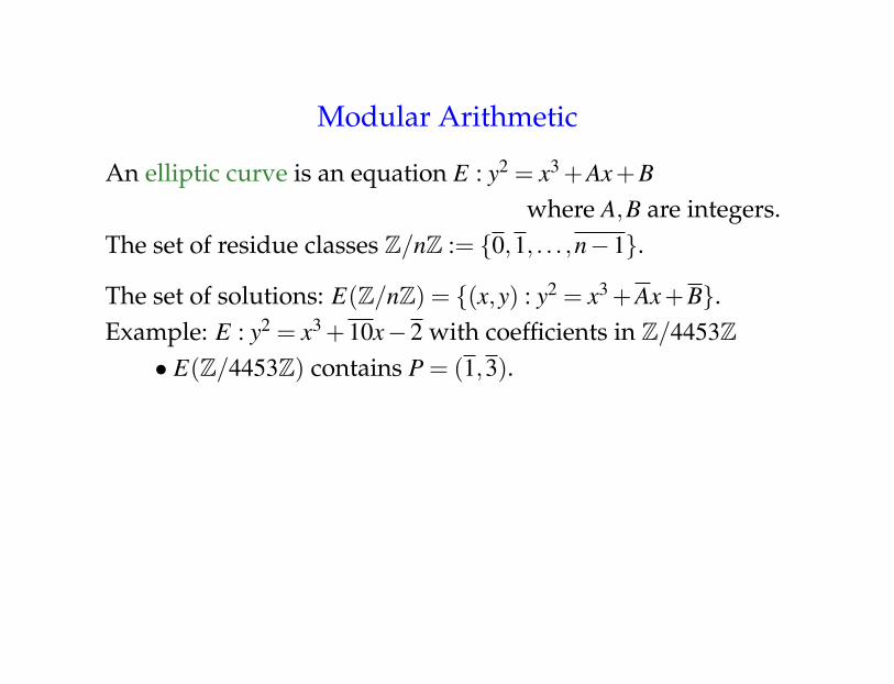
The set of solutions: E(Z/nZ) = {(x,y) : y2 = x3 +Ax+B}.Example: E : y2 = x3 +10x−2 with coefficients in Z/4453Z
• E(Z/4453Z) contains P = (1,3).

Modular Arithmetic
An elliptic curve is an equation E : y2 = x3 +Ax+Bwhere A,B are integers.
The set of residue classes Z/nZ := {0,1, . . . ,n−1}.
The set of solutions: E(Z/nZ) = {(x,y) : y2 = x3 +Ax+B}.Example: E : y2 = x3 +10x−2 with coefficients in Z/4453Z
• E(Z/4453Z) contains P = (1,3).• 2P = (97/62,−1441/63) = (4332,3230).• 3P =(
−8126609828443312 , 262062512821742
43313
), undefined
since 61 is a common factor of 4331 and 4453.
Modular Arithmetic
An elliptic curve is an equation E : y2 = x3 +Ax+Bwhere A,B are integers.
The set of residue classes Z/nZ := {0,1, . . . ,n−1}.
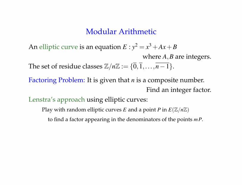
Factoring Problem: It is given that n is a composite number.Find an integer factor.
Lenstra’s approach using elliptic curves:Play with random elliptic curves E and a point P in E(Z/nZ)
to find a factor appearing in the denominators of the points mP.

Modular Arithmetic
An elliptic curve is an equation E : y2 = x3 +Ax+Bwhere A,B are integers.
The set of residue classes Z/nZ := {0,1, . . . ,n−1}.
Factoring Problem: It is given that n is a composite number.Find an integer factor.
Lenstra’s approach using elliptic curves:Play with random elliptic curves E and a point P in E(Z/nZ)
to find a factor appearing in the denominators of the points mP.
Very effective for 60-digit numbersFor larger numbers, effective for finding
prime factors having around 20 to 30 digits

Local-to-Global Principle
An elliptic curve is an equation E : y2 = x3 +Ax+Bwhere A,B are integers.
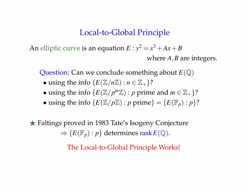
Question: Can we conclude something about E(Q)• using the info {E(Z/nZ) : n ∈ Z+}?• using the info {E(Z/pmZ) : p prime and m ∈ Z+}?• using the info {E(Z/pZ) : p prime}= {E(Fp) : p}?
Local-to-Global Principle
An elliptic curve is an equation E : y2 = x3 +Ax+Bwhere A,B are integers.
Question: Can we conclude something about E(Q)• using the info {E(Z/nZ) : n ∈ Z+}?• using the info {E(Z/pmZ) : p prime and m ∈ Z+}?• using the info {E(Z/pZ) : p prime}= {E(Fp) : p}?
F Faltings proved in 1983 Tate’s Isogeny Conjecture⇒ {E(Fp) : p} determines rankE(Q).
The Local-to-Global Principle Works!
Elliptic Curves
An elliptic curve is an equation E : y2 = x3 +Ax+Bwhere A,B are integers.
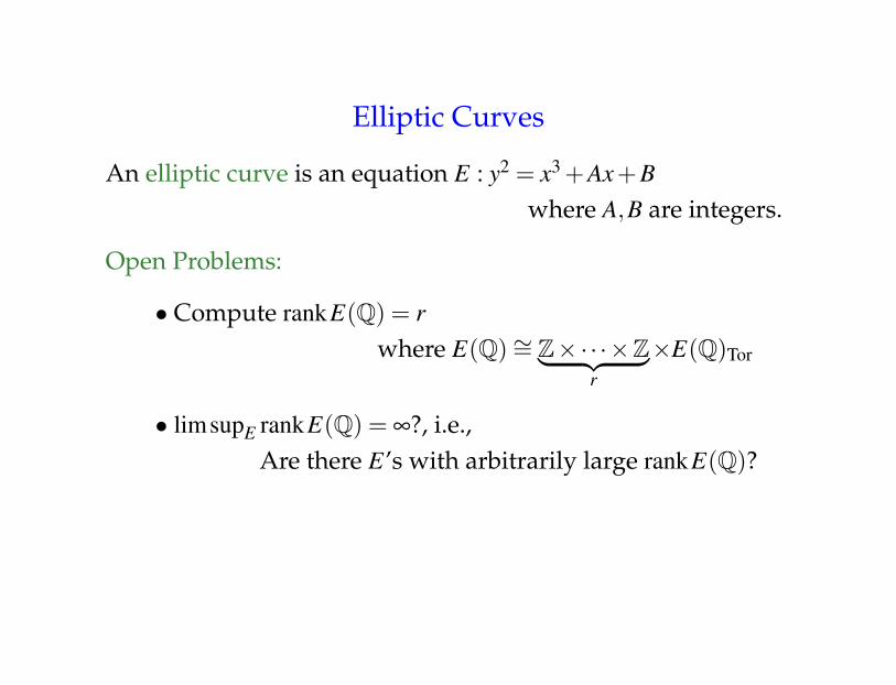
Open Problems:
• Compute rankE(Q) = rwhere E(Q)∼= Z×·· ·×Z︸ ︷︷ ︸
r
×E(Q)Tor
• limsupE rankE(Q) = ∞?, i.e.,Are there E’s with arbitrarily large rankE(Q)?

Elliptic Curves
An elliptic curve is an equation E : y2 = x3 +Ax+Bwhere A,B are integers.
Open Problems:
• Compute rankE(Q) = rwhere E(Q)∼= Z×·· ·×Z︸ ︷︷ ︸
r
×E(Q)Tor
• limsupE rankE(Q) = ∞?, i.e.,Are there E’s with arbitrarily large rankE(Q)?
F (Faltings) {E(Fp) : p} determines rankE(Q).

Birch and Swinnerton-Dyer Conj.
Award: $ 26 ·56

Birch and Swinnerton-Dyer Conj.
Award: $ 26 ·56
Experiment:
∏p<x
′ # E(Fp)p
≈ cE(lnx)rankE(Q)
Birch and Swinnerton-Dyer Conj.
Award: $ 26 ·56
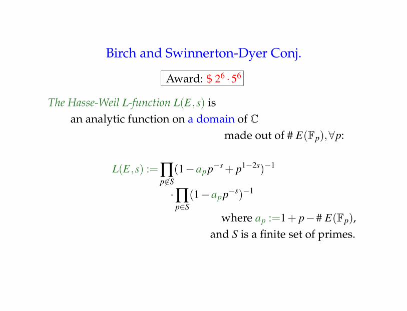
The Hasse-Weil L-function L(E,s) isan analytic function on a domain of C
made out of # E(Fp),∀p:
L(E,s) :=∏p 6∈S
(1−app−s + p1−2s)−1
·∏p∈S
(1−app−s)−1
where ap :=1+ p−# E(Fp),and S is a finite set of primes.
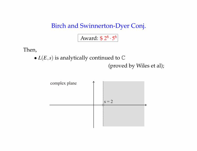
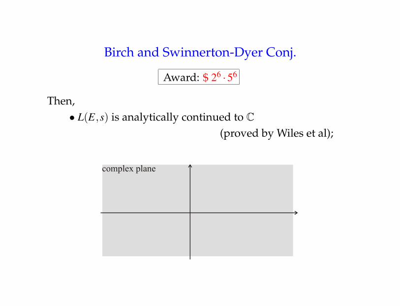
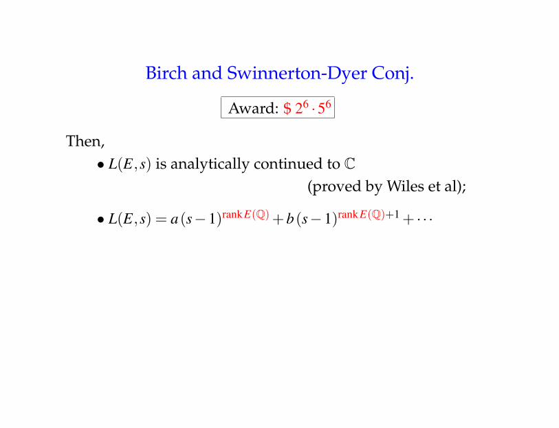
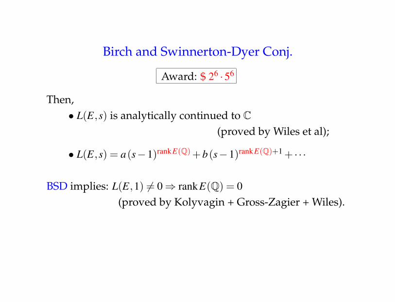
Birch and Swinnerton-Dyer Conj.
Award: $ 26 ·56
Then,• L(E,s) is analytically continued to C
(proved by Wiles et al);
Birch and Swinnerton-Dyer Conj.
Award: $ 26 ·56
Then,• L(E,s) is analytically continued to C
(proved by Wiles et al);
Birch and Swinnerton-Dyer Conj.
Award: $ 26 ·56
Then,• L(E,s) is analytically continued to C
(proved by Wiles et al);
• L(E,s) = a(s−1)rankE(Q) +b(s−1)rankE(Q)+1 + · · ·

Birch and Swinnerton-Dyer Conj.
Award: $ 26 ·56
Then,• L(E,s) is analytically continued to C
(proved by Wiles et al);
• L(E,s) = a(s−1)rankE(Q) +b(s−1)rankE(Q)+1 + · · ·
BSD implies: L(E,1) 6= 0⇒ rankE(Q) = 0
Birch and Swinnerton-Dyer Conj.
Award: $ 26 ·56
Then,• L(E,s) is analytically continued to C
(proved by Wiles et al);
• L(E,s) = a(s−1)rankE(Q) +b(s−1)rankE(Q)+1 + · · ·
BSD implies: L(E,1) 6= 0⇒ rankE(Q) = 0(proved by Kolyvagin + Gross-Zagier + Wiles).

Birch and Swinnerton-Dyer Conj.
Searching for Evidence
Let E be given by y2 = x3 +Ax+B.A quadratic twist of E is an elliptic curve given by
ED : Dy2 = x3 +Ax+Bwhere D is a square-free integer.
rankED(Q) varies as D varies.

Birch and Swinnerton-Dyer Conj.
Searching for Evidence
Let E be given by y2 = x3 +Ax+B.A quadratic twist of E is an elliptic curve given by
ED : Dy2 = x3 +Ax+Bwhere D is a square-free integer.
rankED(Q) varies as D varies.
BSD implies the uniform distribution of the paritiesof rankED(Q).

Birch and Swinnerton-Dyer Conj.
Searching for Evidence
Let E be given by y2 = x3 +Ax+B.A quadratic twist of E is an elliptic curve given by
ED : Dy2 = x3 +Ax+Bwhere D is a square-free integer.
rankED(Q) varies as D varies.
BSD implies the uniform distribution of the paritiesof rankED(Q).
Are the parities of rankED(Q) uniformly distributed?

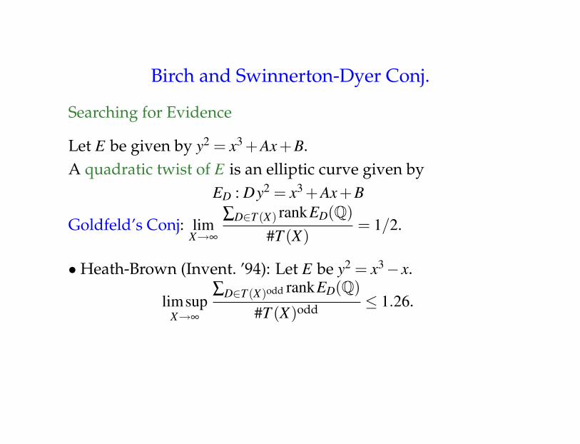
Birch and Swinnerton-Dyer Conj.
Searching for Evidence
Let E be given by y2 = x3 +Ax+B.A quadratic twist of E is an elliptic curve given by
ED : Dy2 = x3 +Ax+B
Goldfeld’s Conj: limX→∞
∑D∈T (X) rankED(Q)#T (X)
= 1/2
T (X) = {0 < |D|< X : D square-free}.
Birch and Swinnerton-Dyer Conj.
Searching for Evidence
Let E be given by y2 = x3 +Ax+B.A quadratic twist of E is an elliptic curve given by
ED : Dy2 = x3 +Ax+B
Goldfeld’s Conj: limX→∞
∑D∈T (X) rankED(Q)#T (X)
= 1/2.
• Heath-Brown (Invent. ’94): Let E be y2 = x3− x.
limsupX→∞
∑D∈T (X)odd rankED(Q)
#T (X)odd ≤ 1.26.
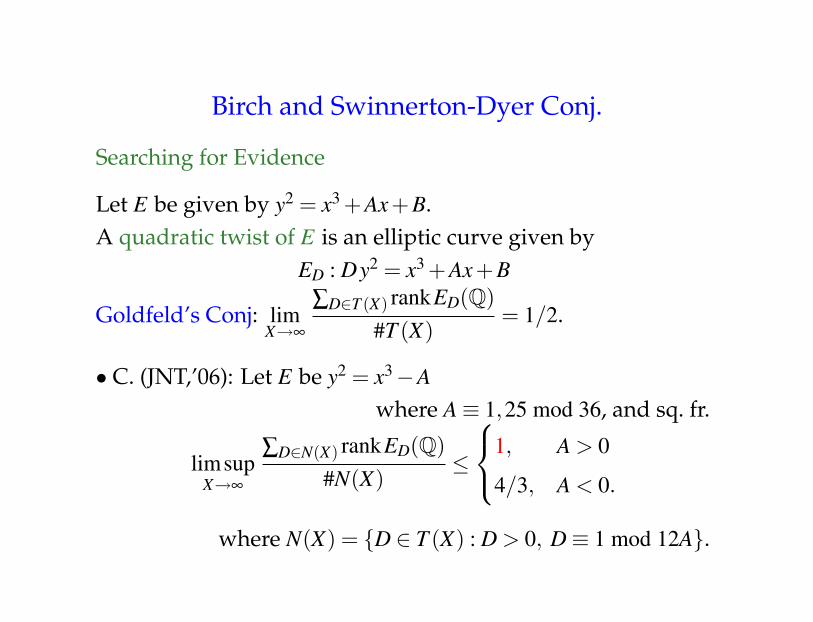
Birch and Swinnerton-Dyer Conj.
Searching for Evidence
Let E be given by y2 = x3 +Ax+B.A quadratic twist of E is an elliptic curve given by
ED : Dy2 = x3 +Ax+B
Goldfeld’s Conj: limX→∞
∑D∈T (X) rankED(Q)#T (X)
= 1/2.
• C. (JNT,’06): Let E be y2 = x3−Awhere A≡ 1,25 mod 36, and sq. fr.
limsupX→∞
∑D∈N(X) rankED(Q)#N(X)
≤
1, A > 0
4/3, A < 0.
where N(X) = {D ∈ T (X) : D > 0, D≡ 1 mod 12A}.

Birch and Swinnerton-Dyer Conj.
Theoretical Results
• J. Coates & A. Wiles (1978):L(E,1) = 0 and E has CM ⇒ rankE(Q)≥ 1.
• A. Wiles at et al: L(E,s), analytically continuedas a corollary of the proof of
the Taniyama-Shimura Conj.
• Kolyvagin + Gross-Zagier: L(E,1) 6= 0⇒ rankE(Q) = 0.
BSD: L(E,s) = a(s−1)rankE(Q) +b(s−1)rankE(Q)+1 + · · ·
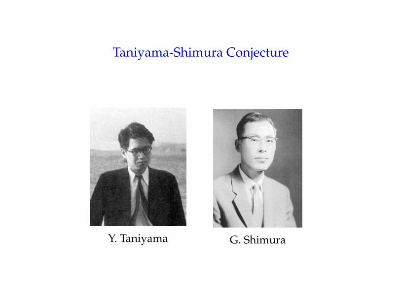
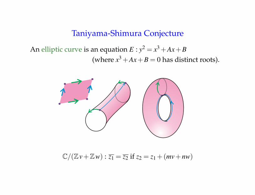
Taniyama-Shimura Conjecture
Y. Taniyama G. Shimura

Taniyama-Shimura Conjecture
An elliptic curve is an equation E : y2 = x3 +Ax+B(where x3 +Ax+B = 0 has distinct roots).
Z/5Z : 1 = 16 since 16 = 1+5×3

Taniyama-Shimura Conjecture
An elliptic curve is an equation E : y2 = x3 +Ax+B(where x3 +Ax+B = 0 has distinct roots).
C/(Zv+Zw) : z1 = z2 if z2 = z1 +(mv+nw)
where m,n ∈ Z.

Taniyama-Shimura Conjecture
An elliptic curve is an equation E : y2 = x3 +Ax+B(where x3 +Ax+B = 0 has distinct roots).
C/(Zv+Zw) : z1 = z2 if z2 = z1 +(mv+nw)
where m,n ∈ Z.
Example: C/(Z i+Z(1+ i)).• 1 = 1+ i = 0 since 1 = (1+ i)+((−1) · i+0 · (1+ i)).• 55+69i = 14i = 0• a+bi = 0 if a,b ∈ Z.

Taniyama-Shimura Conjecture
An elliptic curve is an equation E : y2 = x3 +Ax+B(where x3 +Ax+B = 0 has distinct roots).
C/(Zv+Zw) : z1 = z2 if z2 = z1 +(mv+nw)
Taniyama-Shimura Conjecture
An elliptic curve is an equation E : y2 = x3 +Ax+B(where x3 +Ax+B = 0 has distinct roots).
C/(Zv+Zw) : z1 = z2 if z2 = z1 +(mv+nw)

Taniyama-Shimura Conjecture
An elliptic curve is an equation E : y2 = x3 +Ax+B(where x3 +Ax+B = 0 has distinct roots).

Taniyama-Shimura Conjecture
An elliptic curve is an equation E : y2 = x3 +Ax+B(where x3 +Ax+B = 0 has distinct roots).
What is that E given v and w?
Taniyama-Shimura Conjecture
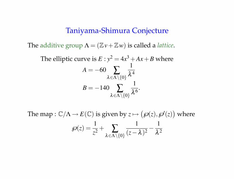
The additive group Λ = (Zv+Zw) is called a lattice.
The elliptic curve is E : y2 = 4x3 +Ax+B where
A =−60 ∑λ∈Λ\{0}
1λ 4
B =−140 ∑λ∈Λ\{0}
1λ 6 .
The map : C/Λ→ E(C) is given by z 7→(℘(z),℘′(z)
)where
℘(z) =1z2 + ∑
λ∈Λ\{0}
1(z−λ )2 −
1λ 2
Taniyama-Shimura Conjecture
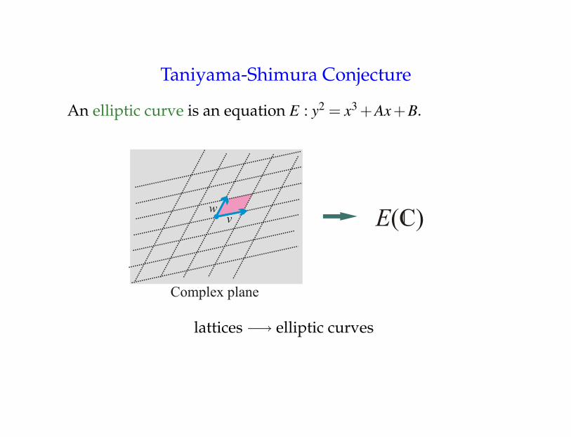
An elliptic curve is an equation E : y2 = x3 +Ax+B.
lattices −→ elliptic curves
Taniyama-Shimura Conjecture
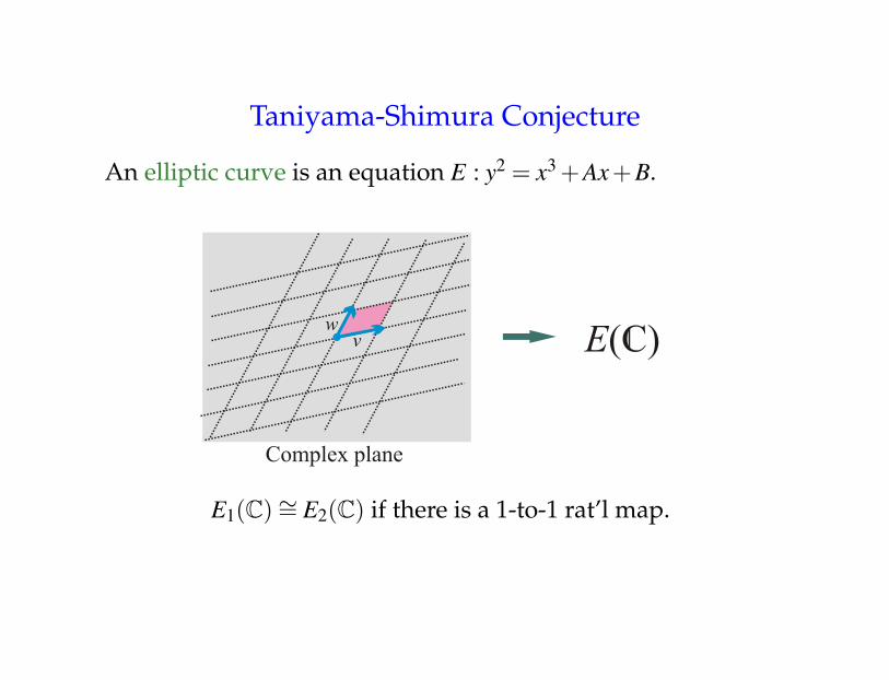
An elliptic curve is an equation E : y2 = x3 +Ax+B.
E1(C)∼= E2(C) if there is a 1-to-1 rat’l map.

Taniyama-Shimura Conjecture
An elliptic curve is an equation E : y2 = x3 +Ax+B.
[E1] = [E2] if there is a 1-to-1 rat’l map.
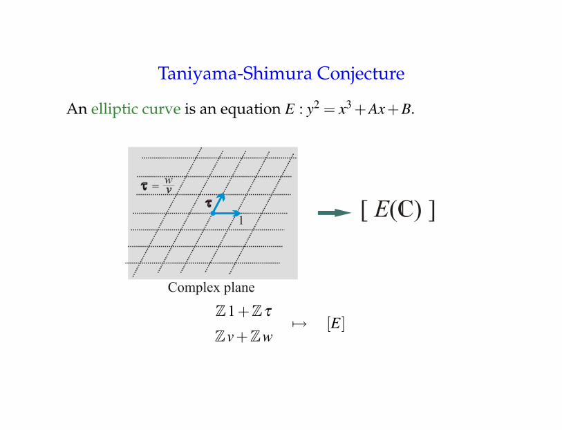
Taniyama-Shimura Conjecture
An elliptic curve is an equation E : y2 = x3 +Ax+B.
Z1+Zτ
Zv+Zw7→ [E]
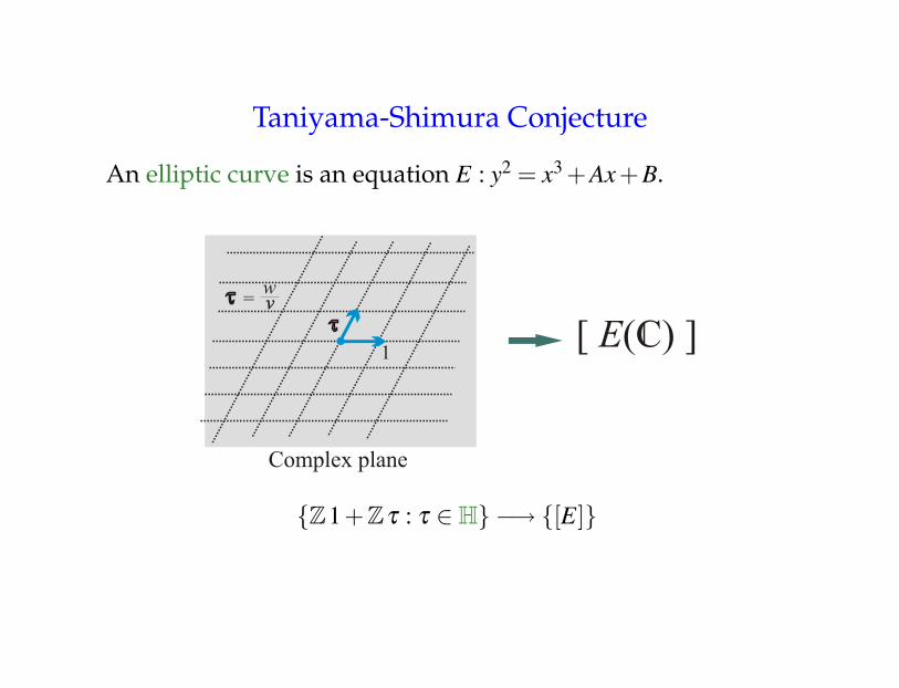
Taniyama-Shimura Conjecture
An elliptic curve is an equation E : y2 = x3 +Ax+B.
{Z1+Zτ : τ ∈H} −→ {[E]}
Taniyama-Shimura Conjecture
An elliptic curve is an equation E : y2 = x3 +Ax+B.
{Z1+Zτ : τ ∈H} −→ {[E]}
Further reductionZ1+Zτ = Zv+Zw for some v and w.
1 = av+bw
τ = cv+dw⇒
(1τ
)=
(a bc d
)(vw
)

Taniyama-Shimura Conjecture
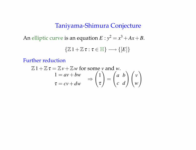
An elliptic curve is an equation E : y2 = x3 +Ax+B.
{Z1+Zτ : τ ∈H} −→ {[E]}
Further reductionZ1+Zτ = Zv+Zw for some v and w.
1 = av+bw
τ = cv+dw⇒
(1τ
)=
(a bc d
)(vw
)(
a bc d
)is invertible!(
a bc d
)is in SL2(Z)
Taniyama-Shimura Conjecture
An elliptic curve is an equation E : y2 = x3 +Ax+B.
{Z1+Zτ : τ ∈H} −→ {[E]}
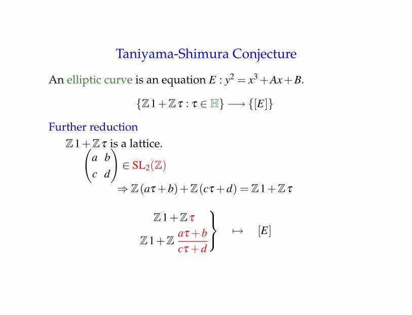
Further reductionZ1+Zτ is a lattice.(
a bc d
)∈ SL2(Z)
⇒ Z(aτ +b)+Z(cτ +d) = Z1+Zτ
If Z(aτ +b)+Z(cτ +d) 7→ E, then
Z1+Zaτ +bcτ +d
7→ [E]
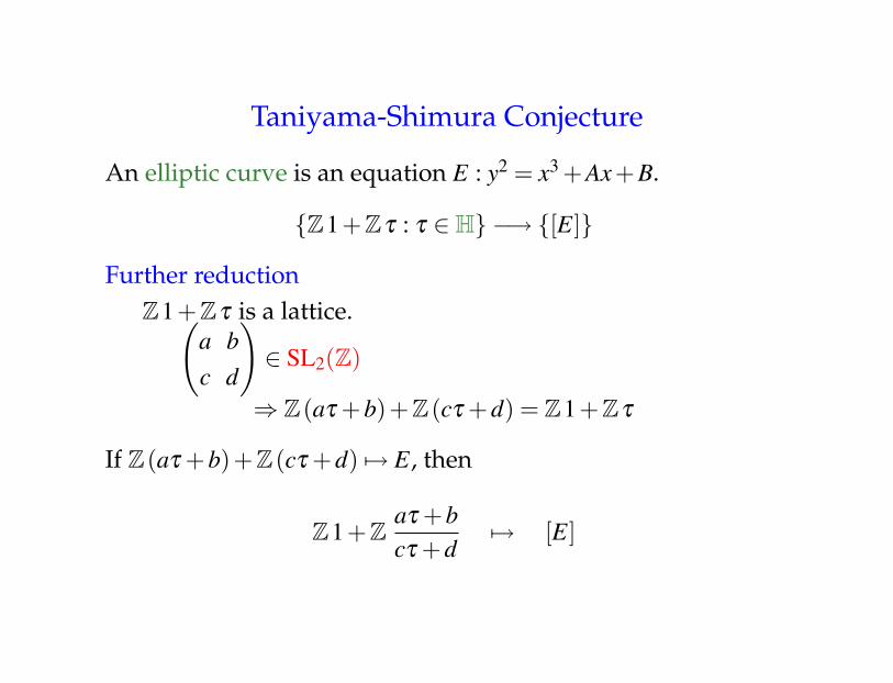
Taniyama-Shimura Conjecture
An elliptic curve is an equation E : y2 = x3 +Ax+B.
{Z1+Zτ : τ ∈H} −→ {[E]}
Further reductionZ1+Zτ is a lattice.(
a bc d
)∈ SL2(Z)
⇒ Z(aτ +b)+Z(cτ +d) = Z1+Zτ
Z1+Zτ
Z1+Zaτ +bcτ +d
7→ [E]

Taniyama-Shimura Conjecture
An elliptic curve is an equation E : y2 = x3 +Ax+B.
{Z1+Zτ : τ ∈H} −→ {[E]}H−→ {[E]}
The quotient group SL2(Z)\H is the equivalence classes [τ] s.t.
[τ] =[
aτ +bcτ +d
]where
(a bc d
)∈ SL2(Z)

Taniyama-Shimura Conjecture
An elliptic curve is an equation E : y2 = x3 +Ax+B.
[τ] =[
aτ +bcτ +d
]

Taniyama-Shimura Conjecture
Modular Forms of weight k
The map: H→{E} is given byτ 7→ E : y2 = 4x3 +A(τ)x+B(τ).
Thus, A(τ) and B(τ) are functions: H→ C.
It turns out that
A(
aτ +bcτ +d
)= (cτ +d)4A(τ)
B(
aτ +bcτ +d
)= (cτ +d)6B(τ)

Taniyama-Shimura Conjecture
Modular Forms of weight k
The map: H→{E} is given byτ 7→ E : y2 = 4x3 +A(τ)x+B(τ).
Thus, A(τ) and B(τ) are functions: H→ C.
It turns out that
A(
aτ +bcτ +d
)= (cτ +d)4A(τ)
B(
aτ +bcτ +d
)= (cτ +d)6B(τ)
The function A(τ) is called a modular form of weight 4,and B(τ), a modular form of weight 6.
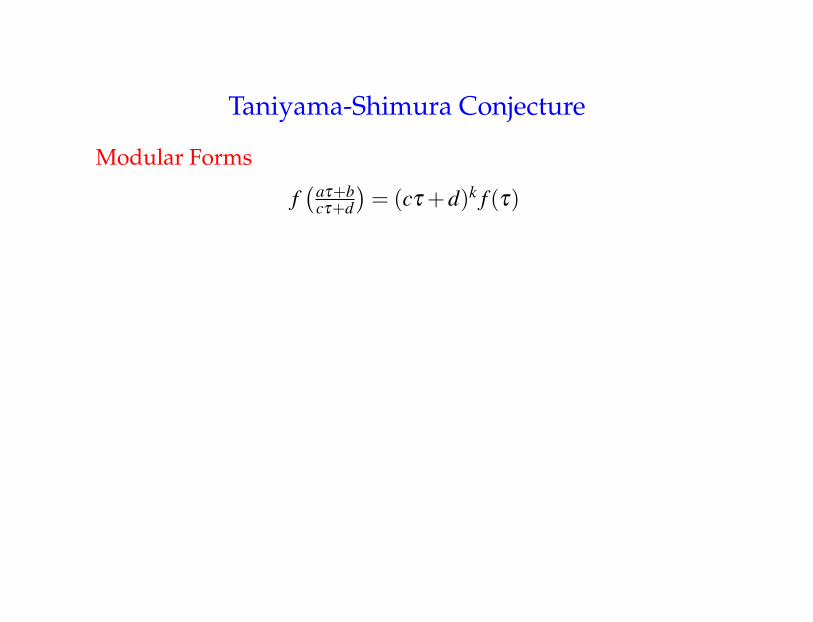
Taniyama-Shimura Conjecture
Modular Forms
f(aτ+b
cτ+d
)= (cτ +d)k f (τ)

Taniyama-Shimura Conjecture
Modular Forms
f(aτ+b
cτ+d
)= (cτ +d)k f (τ)
Modular Functions
f(aτ+b
cτ+d
)= f (τ)

Taniyama-Shimura Conjecture
Modular Forms
f(aτ+b
cτ+d
)= (cτ +d)k f (τ)
Modular Functions
f(aτ+b
cτ+d
)= f (τ)
Example:
j(τ) =−1728A(τ)3
27B(τ)2−A(τ)3 where
A(aτ+b
cτ+d
)= (cτ +d)4A(τ)
B(aτ+b
cτ+d
)= (cτ +d)6B(τ)
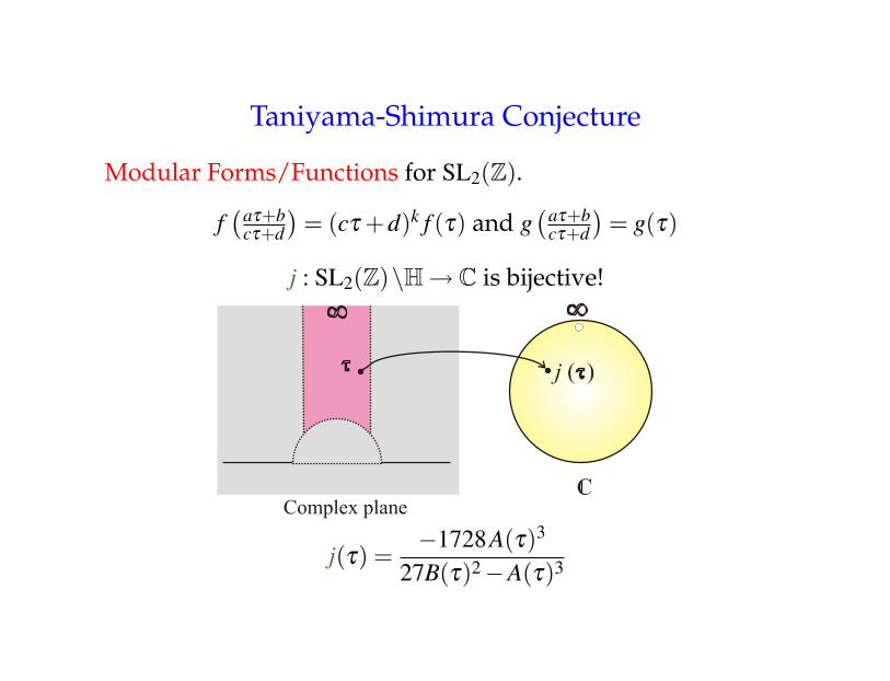
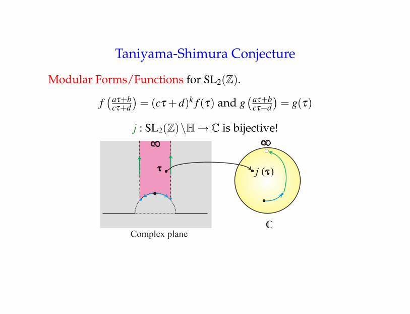
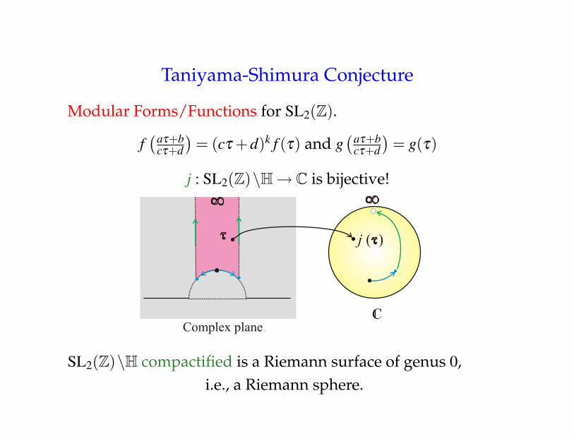
Taniyama-Shimura Conjecture
Modular Forms/Functions for SL2(Z).
f(aτ+b
cτ+d
)= (cτ +d)k f (τ) and g
(aτ+bcτ+d
)= g(τ)
j : SL2(Z)\H→ C is bijective!
j(τ) =−1728A(τ)3
27B(τ)2−A(τ)3
Taniyama-Shimura Conjecture
Modular Forms/Functions for SL2(Z).
f(aτ+b
cτ+d
)= (cτ +d)k f (τ) and g
(aτ+bcτ+d
)= g(τ)
j : SL2(Z)\H→ C is bijective!
j(τ) =−1728A(τ)3
27B(τ)2−A(τ)3
Taniyama-Shimura Conjecture
Modular Forms/Functions for SL2(Z).
f(aτ+b
cτ+d
)= (cτ +d)k f (τ) and g
(aτ+bcτ+d
)= g(τ)
j : SL2(Z)\H→ C is bijective!
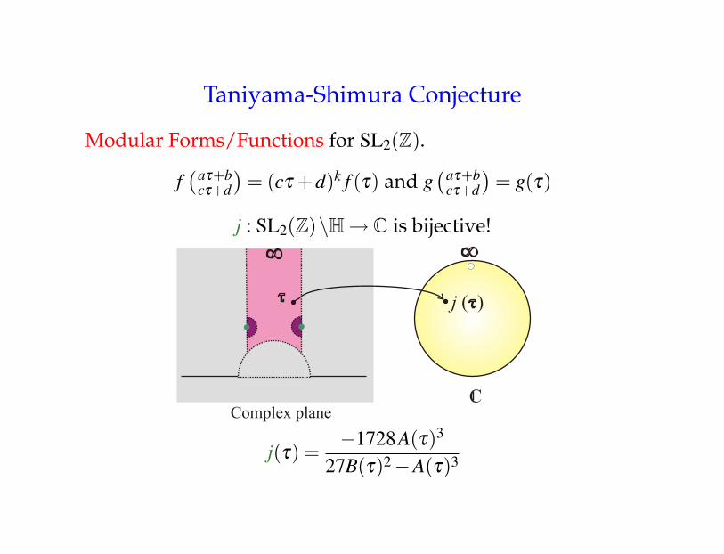
Taniyama-Shimura Conjecture
Modular Forms/Functions for SL2(Z).
f(aτ+b
cτ+d
)= (cτ +d)k f (τ) and g
(aτ+bcτ+d
)= g(τ)
j : SL2(Z)\H→ C is bijective!
SL2(Z)\H compactified is a Riemann surface of genus 0,i.e., a Riemann sphere.

Taniyama-Shimura Conjecture
Modular Forms/Functions for SL2(Z).
f(aτ+b
cτ+d
)= (cτ +d)k f (τ) and g
(aτ+bcτ+d
)= g(τ)
j : SL2(Z)\H→ C is bijective!
The manifold SL2(Z)\H as the solutions of an equation:(SL2(Z)\H)∼= Y (C)
given by [τ] 7→(
j(τ), j(τ))where Y : x− y = 0.
(SL2(Z)\H)∗ ∼= X(C)where X(C) is the compactification of Y (C).
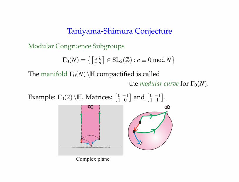
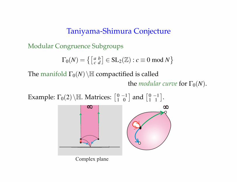
Taniyama-Shimura Conjecture
Modular Congruence Subgroups
Γ0(N) ={[
a bc d
]∈ SL2(Z) : c≡ 0 mod N
}The manifold Γ0(N)\H compactified is called
the modular curve for Γ0(N).
Example: Γ0(2)\H. Matrices:[
0 −11 0
]and
[0 −11 1
].
Taniyama-Shimura Conjecture
Modular Congruence Subgroups
Γ0(N) ={[
a bc d
]∈ SL2(Z) : c≡ 0 mod N
}The manifold Γ0(N)\H compactified is called
the modular curve for Γ0(N).
Example: Γ0(2)\H. Matrices:[
0 −11 0
]and
[0 −11 1
].

Taniyama-Shimura Conjecture
Modular Congruence Subgroups
Γ0(N) ={[
a bc d
]∈ SL2(Z) : c≡ 0 mod N
}The manifold Γ0(N)\H compactified is called
the modular curve for Γ0(N).
Example: Γ0(2)\H. Matrices:[
0 −11 0
]and
[0 −11 1
].
Taniyama-Shimura Conjecture
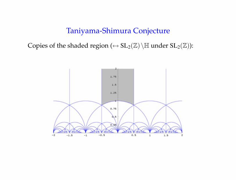
Copies of the shaded region (↔ SL2(Z)\H under SL2(Z)):

Taniyama-Shimura Conjecture
Example: Γ0(16)\H has genus 0.

Taniyama-Shimura Conjecture
Modular Congruence Subgroups
Γ0(N) ={[
a bc d
]∈ SL2(Z) : c≡ 0 mod N
}The manifold Γ0(N)\H compactified is called
the modular curve for Γ0(N).
Example:• Γ0(11)\H has genus 1, i.e., an elliptic curve.• Γ0(22)\H has genus 2.

Taniyama-Shimura Conjecture
Modular Congruence Subgroups
Γ0(N) ={[
a bc d
]∈ SL2(Z) : c≡ 0 mod N
}Modular Forms/Functions for Γ0(N):
f(aτ+b
cτ+d
)= (cτ +d)k f (τ) and g
(aτ+bcτ+d
)= g(τ)
where[
a bc d
]∈ Γ0(N).
Γ0(N)\Hg : Γ0(N)\H−→ C
Taniyama-Shimura Conjecture
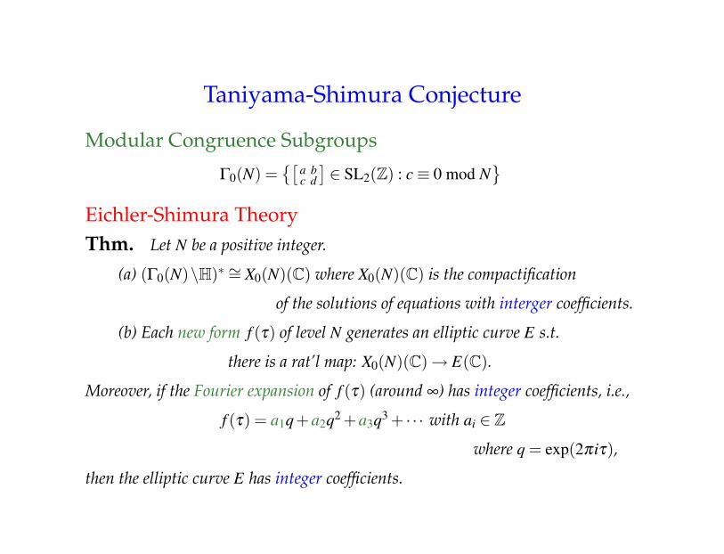
Modular Congruence Subgroups
Γ0(N) ={[
a bc d
]∈ SL2(Z) : c≡ 0 mod N
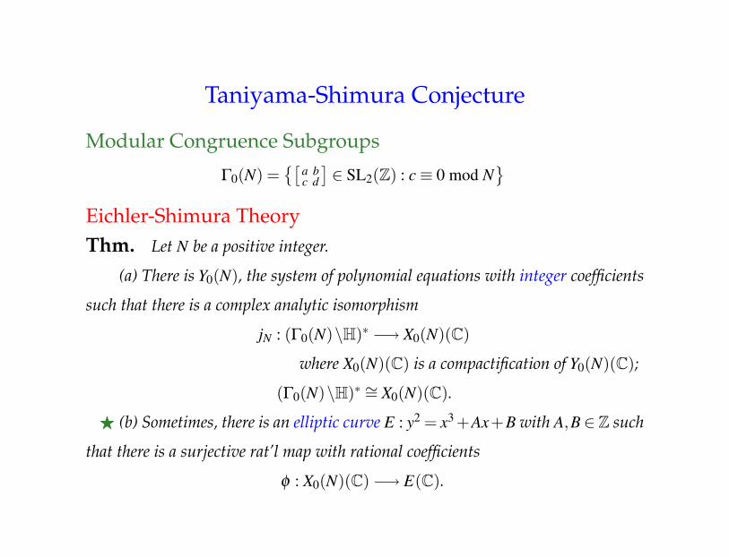
}Eichler-Shimura TheoryThm. Let N be a positive integer.
(a) There is Y0(N), the system of polynomial equations with integer coefficients
such that there is a complex analytic isomorphism
jN : (Γ0(N)\H)∗ −→ X0(N)(C)
where X0(N)(C) is a compactification of Y0(N)(C);
(Γ0(N)\H)∗ ∼= X0(N)(C).
F (b) Sometimes, there is an elliptic curve E : y2 = x3 +Ax+B with A,B∈Z such
that there is a surjective rat’l map with rational coefficients
φ : X0(N)(C)−→ E(C).
Taniyama-Shimura Conjecture
Modular Congruence Subgroups
Γ0(N) ={[
a bc d
]∈ SL2(Z) : c≡ 0 mod N
}Eichler-Shimura Theory Given N, sometimes
∃ a nice way to construct an elliptic curve Eusing X0(N).

Taniyama-Shimura Conjecture
Modular Congruence Subgroups
Γ0(N) ={[
a bc d
]∈ SL2(Z) : c≡ 0 mod N
}Eichler-Shimura Theory Given N, sometimes
∃ a nice way to construct an elliptic curve Eusing X0(N).
Sometimes, ∃ a special modular form f of weight 2 for Γ0(N),called a new form of level N. Consider the map Ψ f : Γ0(N)→Cgiven by [
a bc d
]7→
∫ aτ0+bcτ0+d
τ0
f (z) dz.
Then, Ψ f (Γ0(N)) is ...
Taniyama-Shimura Conjecture
Modular Congruence Subgroups
Γ0(N) ={[
a bc d
]∈ SL2(Z) : c≡ 0 mod N
}Eichler-Shimura Theory Given N, sometimes
∃ a nice way to construct an elliptic curve Eusing X0(N).
Sometimes, ∃ a special modular form f of weight 2 for Γ0(N),called a new form of level N. Consider the map Ψ f : Γ0(N)→Cgiven by [
a bc d
]7→
∫ aτ0+bcτ0+d
τ0
f (z) dz.
Then, Ψ f (Γ0(N)) is ...a lattice Zv+Zw, an elliptic curve.
Taniyama-Shimura Conjecture
Modular Congruence Subgroups
Γ0(N) ={[
a bc d
]∈ SL2(Z) : c≡ 0 mod N
}Eichler-Shimura TheoryThm. Let N be a positive integer.
(a) (Γ0(N)\H)∗ ∼= X0(N)(C) where X0(N)(C) is the compactification
of the solutions of equations with interger coefficients.
(b) Each new form f (τ) of level N generates an elliptic curve E s.t.
there is a rat’l map: X0(N)(C)→ E(C).
Moreover, if the Fourier expansion of f (τ) (around ∞) has integer coefficients, i.e.,
f (τ) = a1q+a2q2 +a3q3 + · · · with ai ∈ Z
where q = exp(2πiτ),
then the elliptic curve E has integer coefficients.

Taniyama-Shimura Conjecture
Modular Congruence Subgroups
Γ0(N) ={[
a bc d
]∈ SL2(Z) : c≡ 0 mod N
}Eichler-Shimura TheoryThm. Let N be a positive integer.
(a) (Γ0(N)\H)∗ ∼= X0(N)(C)where X0(N)(C) is the compactification
of the solutions of equations with interger coefficients.(b) {new forms}→ {E}, and
{new forms with Z-coeff.}→ {E with Z-coeff.}X0(N)−→ E
Taniyama-Shimura Conjecture
Modular Congruence Subgroups
Γ0(N) ={[
a bc d
]∈ SL2(Z) : c≡ 0 mod N
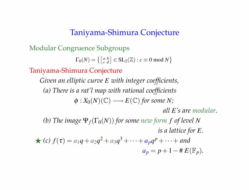
}Taniyama-Shimura Conjecture
Given an elliptic curve E with integer coefficients,(a) There is a rat’l map with rational coefficients
φ : X0(N)(C)−→ E(C) for some N;all E’s are modular.
(b) The image Ψ f (Γ0(N)) for some new form f of level Nis a lattice for E.
F (c) f (τ) = a1q+a2q2 +a3q3 + · · ·+apqp + · · ·+ andap = p+1−# E(Fp).
Taniyama-Shimura Conjecture
Modular Congruence Subgroups
Γ0(N) ={[
a bc d
]∈ SL2(Z) : c≡ 0 mod N
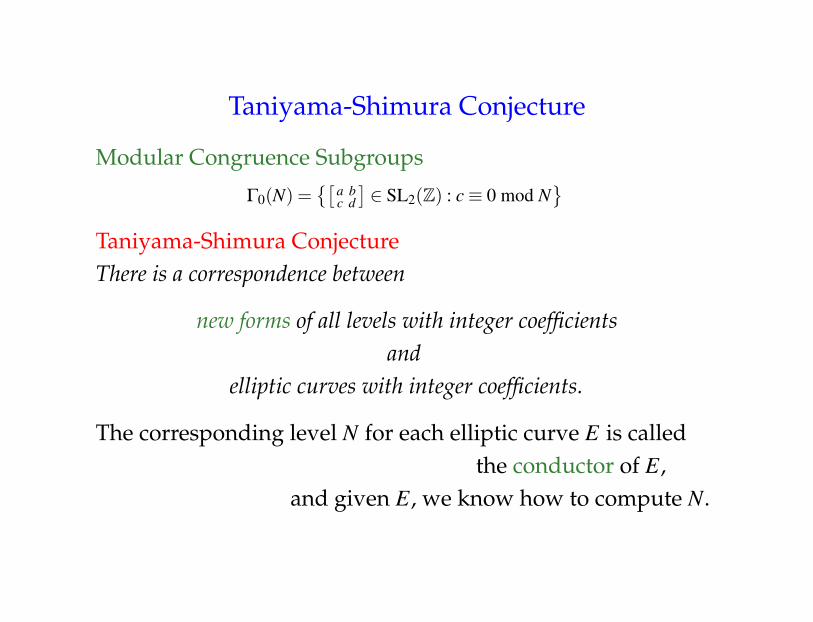
}Taniyama-Shimura ConjectureThere is a correspondence between
new forms of all levels with integer coefficientsand
elliptic curves with integer coefficients.
The corresponding level N for each elliptic curve E is calledthe conductor of E,
and given E, we know how to compute N.
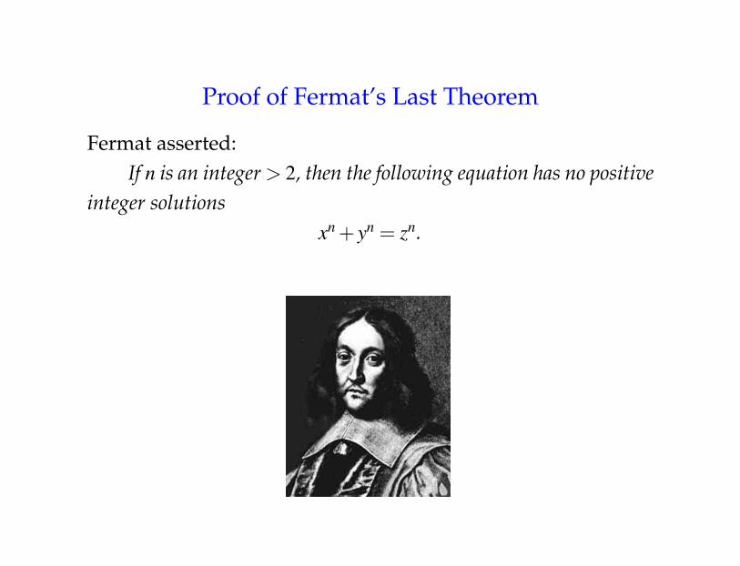
Proof of Fermat’s Last Theorem
Fermat asserted:If n is an integer > 2, then the following equation has no positive
integer solutionsxn + yn = zn.
Proof of Fermat’s Last Theorem
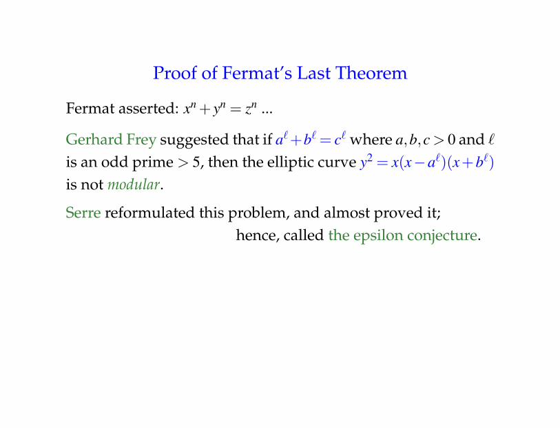
Fermat asserted: xn + yn = zn ...
Gerhard Frey suggested that if a`+b` = c` where a,b,c > 0 and `
is an odd prime > 5, then the elliptic curve y2 = x(x−a`)(x+b`)is not modular.
Serre reformulated this problem, and almost proved it;hence, called the epsilon conjecture.

Proof of Fermat’s Last Theorem
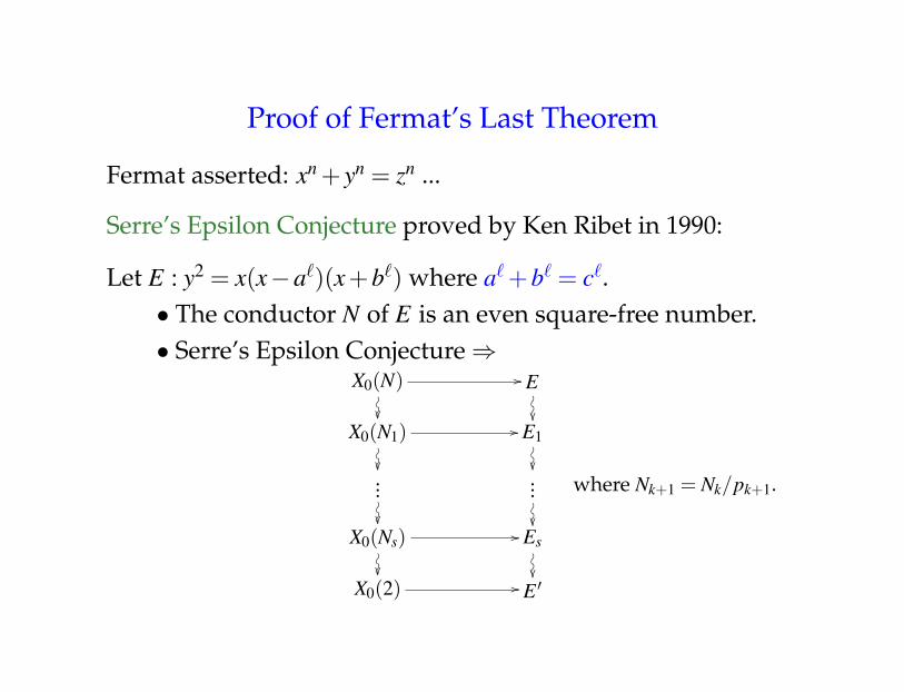
Fermat asserted: xn + yn = zn ...
Serre’s Epsilon Conjecture proved by Ken Ribet in 1990:
Let E : y2 = x(x−a`)(x+b`) where a` +b` = c`.• The conductor N of E is an even square-free number.• Serre’s Epsilon Conjecture ⇒
X0(N) //
�� �O�O�O
E
�� �O�O�O�O
X0(N′) // E ′
where N′ = N/p for any odd prime p.
Proof of Fermat’s Last Theorem
Fermat asserted: xn + yn = zn ...
Serre’s Epsilon Conjecture proved by Ken Ribet in 1990:
Let E : y2 = x(x−a`)(x+b`) where a` +b` = c`.• The conductor N of E is an even square-free number.• Serre’s Epsilon Conjecture ⇒
X0(N) //
���O�O
E
���O�O
X0(N1) //
���O�O
E1
���O�O
...���O�O
...���O�O
X0(Ns) //
���O�O
Es
���O�O
X0(2) // E ′
where Nk+1 = Nk/pk+1.
Proof of Fermat’s Last Theorem
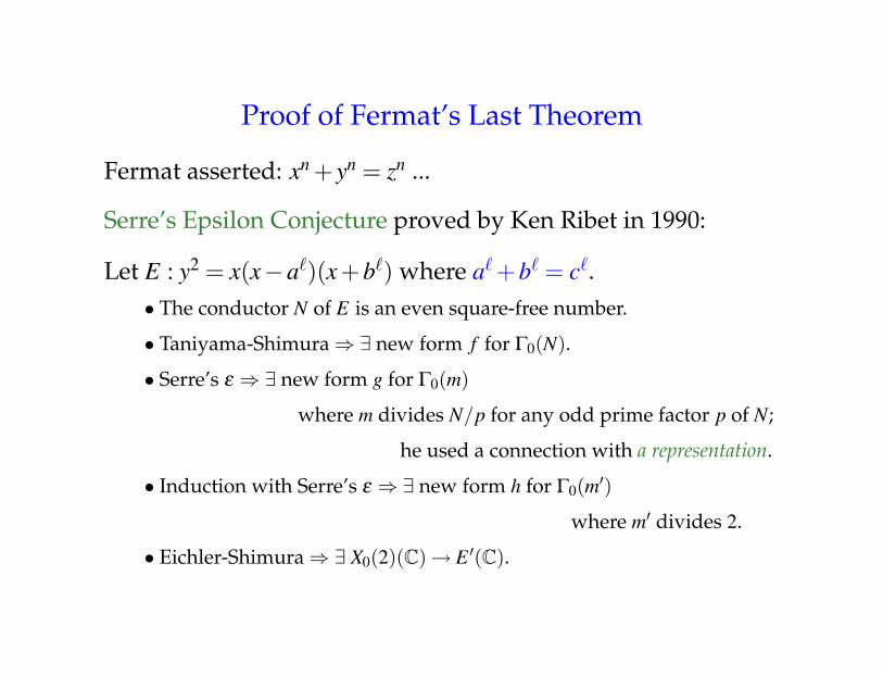
Fermat asserted: xn + yn = zn ...
Serre’s Epsilon Conjecture proved by Ken Ribet in 1990:
Let E : y2 = x(x−a`)(x+b`) where a` +b` = c`.• The conductor N of E is an even square-free number.
• Taniyama-Shimura ⇒ ∃ new form f for Γ0(N).
• Serre’s ε ⇒ ∃ new form g for Γ0(m)
where m divides N/p for any odd prime factor p of N;
he used a connection with a representation.
• Induction with Serre’s ε ⇒ ∃ new form h for Γ0(m′)
where m′ divides 2.
• Eichler-Shimura ⇒ ∃ X0(2)(C)→ E ′(C).

Proof of Fermat’s Last Theorem
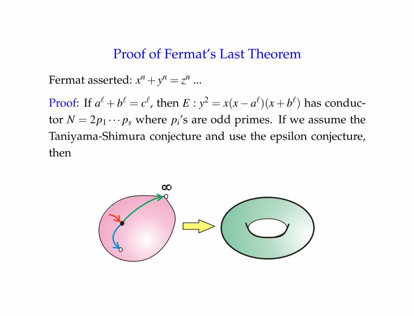
Fermat asserted: xn + yn = zn ...
Proof: If a` + b` = c`, then E : y2 = x(x− a`)(x + b`) has conduc-tor N = 2p1 · · · ps where pi’s are odd primes. If we assume theTaniyama-Shimura conjecture and use the epsilon conjecture,then
X0(2)(C)−→ E ′(C)where is E ′ is an elliptic curve.
X0(2) =?

Proof of Fermat’s Last Theorem
Fermat asserted: xn + yn = zn ...
Proof: If a` + b` = c`, then E : y2 = x(x− a`)(x + b`) has conduc-tor N = 2p1 · · · ps where pi’s are odd primes. If we assume theTaniyama-Shimura conjecture and use the epsilon conjecture,then
X0(2)(C)−→ E ′(C)where is E ′ is an elliptic curve.
X0(2) =?(Γ0(2)\H
)∗ ∼= X0(2)
Proof of Fermat’s Last Theorem
Fermat asserted: xn + yn = zn ...
Proof: If a` + b` = c`, then E : y2 = x(x− a`)(x + b`) has conduc-tor N = 2p1 · · · ps where pi’s are odd primes. If we assume theTaniyama-Shimura conjecture and use the epsilon conjecture,then

Proof of Fermat’s Last Theorem
Fermat asserted: xn + yn = zn ...
Proof: If a` + b` = c`, then E : y2 = x(x− a`)(x + b`) has conduc-tor N = 2p1 · · · ps where pi’s are odd primes. If we assume theTaniyama-Shimura conjecture and use the epsilon conjecture,then
Q.E.D.

Serre’s Conjecture
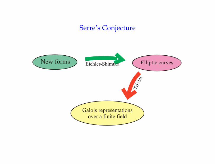
Serre’s Conjecture
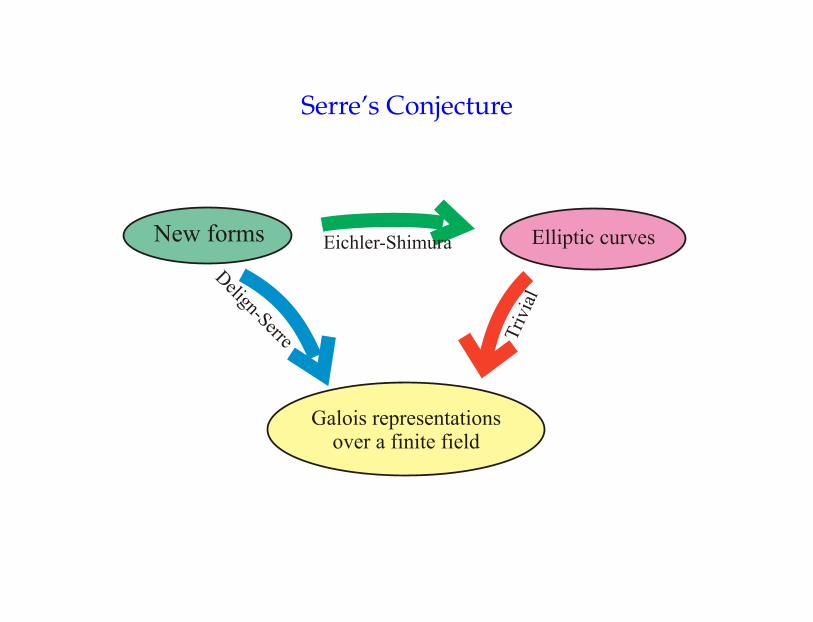
Serre’s Conjecture

Serre’s Conjecture

Serre’s Conjecture
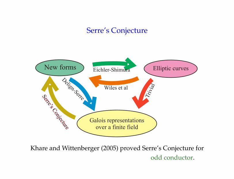
Serre’s Conjecture
Khare and Wittenberger (2005) proved Serre’s Conjecture forodd conductor.
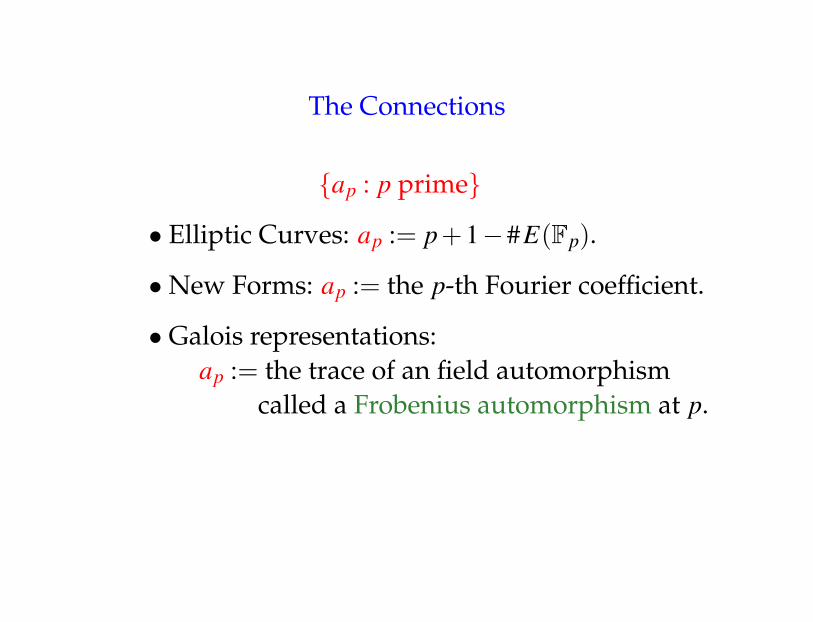
The Connections
{ap : p prime}
• Elliptic Curves: ap := p+1−#E(Fp).
• New Forms: ap := the p-th Fourier coefficient.
• Galois representations:ap := the trace of an field automorphism
called a Frobenius automorphism at p.