1

THE ANSI/ANS STANDARD 58.2-1988: TWO-PHASE JET MODEL Graham Wallis September 15, 2004 Introduction For some time I have been curious about the origins of the two-phase jet model that appears in Appendix C of the ANSI/ANS Standard1. It is given there as a set of formulae, with almost no technical explanation. The key reference is to an EPRI report, NP-4418 (Healzer and Singh, 1986). Ralph Caruso asked EPRI for a copy and was told that they could not locate one. There is no copy in the ANL library and ANL were unable to obtain one through interlibrary loan. Perhaps this report only existed in draft form and was never formally issued. Ralph found another related report2, (Healzer and Elias, EPRI NP-4362, 1986) which is the final report of work performed under EPRI Project Manager Avtar Singh. The equations given in the Standard are not derived in this report, but there is a good presentation of the modeling of an expanding supersonic jet using the method of characteristics. This is combined with a shock wave model to predict the pressure distributions on targets in the Marviken tests. Bill Shack found an earlier report3 (Elias et al, 1984) also describing a jet model based on the method of characteristics. Another useful reference is the Sandia report4, (Weigand et al) NUREG/CR-2913) that was discussed in the ACRS letter of ….. The approximate model presented there for the initial stage of the jet appears to be the same as that adopted in the Standard. Victor Ransom has been conducting a parallel critique9. It provides some nice pictures of the reality of supersonic jets and makes some comments generally in agreement with mine. This memo critiques the methods described in the Standard, compares them with the referenced technical models and the probable reality, and also with independent calculations. The work has been performed quickly in order to

2

provide input to the forthcoming ACRS Thermal/hydraulics Subcommittee meeting and may contain errors or misunderstandings. It is concluded that there are (at least) several problematic areas with the methods in the Standard: 1. The overall description of the jet flow pattern is at odds with the reality of supersonic jet flow. 2. The "jet pressure" is not defined. It seems to mean different things in different "Regions" of the jet. Some of the assumed profiles are inconsistent with reality, giving the inverse of what actually occurs in parts of the jet that are overexpanded. The impact pressures in the far field may be overestimated. 3. The use of one-dimensional assumptions leads to errors in predicting the "asymptotic plane" where supersonic effects are supposed to end. Besides the fact that such a plane does not exist and supersonic effects persist to many more L/Ds, these assumptions lead to a spread by a factor of four in the prediction, depending on how the assumptions are manipulated. 4. The use of stagnation conditions to compute the quality in the flow at the "asymptotic plane" is erroneous. The mixture is actually traveling at high Mach Number when atmospheric pressure is reached on the average for the first time. The Sandia Report Sandia4 performed CFD calculations of a jet issuing into a space between two parallel planes. They assumed the two-phase flow to be homogeneous and in thermodynamic equilibrium. They derived contours of constant pressure, velocity vectors and pressures on the large target, as shown in the attached figures for a discharge of water initially saturated at 150bar. This is a confined jet and not the free jet expected from a break following a LOCA. The analysis is quite complete and impressive but detailed results are only presented for L/D =2. It is therefore not shown how the flow behaves when the plate is far enough away from the nozzle for the flow to behave more like what would be obtained with a free jet.

3

Figure 1 shows a "core" region in which there is no depressurization, rather than the usual situation where choking occurs at the exit plane. This may be a real effect as there is evidence from the Marviken tests of a region near the break where the stagnation pressure is fully recoverable; it doesn't matter for the far field at large distances from the break.

Figure 1 Pressure contours for a jet issuing between two discs4 The jet is able to turn 900 and follow the inner wall, executing the familiar Prandtl-Meyer expansion. The contours of constant pressure near the nozzle resemble those from a point source to some extent. Figure 2 shows the corresponding velocity vectors. The supersonic flow undergoes a shock as it approaches the target plate. The shock is normal near the stagnation point and oblique further out. The calculation is not

4

continued to the "outside world" at large radius, but presumably there would have to be another shock wave to enable the flow to get out of the disc-like slot into an atmosphere at 1bar.

Figure 2 Velocity vectors corresponding to Figure 1 Figure 3 shows the pressure distribution on the large target disc. The pressure is seen to fall off with radius. Since the flow is inviscid in this model, the streamlines from the stagnation point flow along the surface, conserving stagnation pressure. This would be the maximum pressure felt by an object placed anywhere close to the target surface and it would be the same at all radii. For example, at R/D =2, the static pressure on the target plate is about 5bar, but an object near the plate would experience the full stagnation pressure of 18bar.

5

Figure 3 Pressure distribution along the target plate4

Sandia4 also discuss the problem of a free jet issuing for a tube, rather than from a hole in a disc. This is not analyzed using CFD but an approximate solution is presented. It is assumed, without much explanation (p.89) that the jet "has a well-defined boundary described by a 450 expansion angle". This is despite the 900 turning angle obtained with the confined jet. It is assumed that the flow can be treated as one-dimensional in the 450 cone (this is a stretch of one-dimensionality). This enables the velocity and thermodynamic properties to be computed, assuming an isentropic expansion. Then the pressure on the plate is determined by using the normal shock relations at the stagnation point and oblique shock relations further out along the plate (which is at odds with the one-dimensional model used to

6

calculate the velocity. The explanation of this is not particularly clear). The calculated pressures come quite close to experimental measurements for L/D less than about 5. They also seem to be quite close to the pressures computed on the plate in the confined jet situation, though this appears to be a somewhat different problem. As pointed out in our letter, the pressures recorded on a large plate at some radius are not the same as the pressures that would be encountered by a small object placed at the same position, in the absence of a plate. In a region close to the nozzle, the confined jet and the free jet would be expected to behave the same. This is because the flow is supersonic and the free jet core "doesn't know" the conditions on the free boundary or at the target until waves have propagated in from those boundaries to convey the information that they are there. The ANSI/ANS Standard A very brief description of the model is presented in Appendix C. Figure C-1 delineates three regions, shown here in Figure 4. Region 1 is the core region, as in the Sandia report. Its length appears to be described by using a correlation developed in reference 4. The length depends on the upstream subcooling.

7

Figure 4 Jet model in the ANSI/ANS Standard Region 2 follows the 450 cone assumed by Sandia. It ends at an "asymptotic area". For low subcooling this is where the pressure is predicted to be atmospheric. The area, Aa of the jet at this plane is computed from Aa/Ae = Ge

2 /(ρa CT P0) (C-3) (I refuse to include a units factor gc!) The symbols have their usual meaning. The thrust coefficient times the stagnation pressure, CTP0 , is the same as the momentum flux in the jet, or

8

Aaρava2. Since from continuity, Aaρava = Aeρaeve, and Ge = ρeve , (C-3) is the

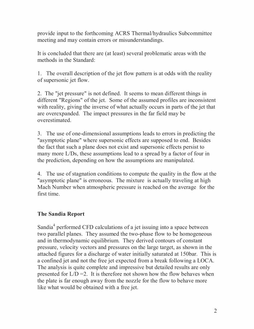
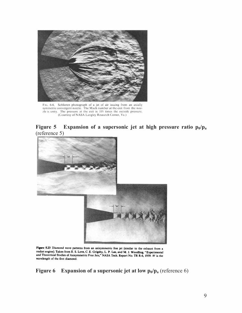
same as the continuity equation Aaρava = Aeρaeve (1) Use of (1) is the same as using the simple one-dimensional equations for isentropic flow to compute the area where the pressure drops to atmospheric. From geometry, for the assumed 450 jet boundary, the distance from the break plane to the asymptotic plane is La/De = 1/2 ((Aa/Ae)0.5 - 1) = 1/2 (Da/De -1) (C-5) In Region 3, "interaction with the surrounding environment is assumed to start" and the jet is then assumed to expand with a 10 degree exterior half-angle after the "asymptotic plane". There is no discussion of shock waves forming in front of obstacles. The assumption seems to be that all supersonic effects are over at the end of Region 2 and the jet behavior is thereafter governed by turbulent mixing with the surrounding fluid. The concept that supersonic expansion stops at an "asymptotic plane" is not consistent with observation. In the Marviken tests, and according to theory, the mean pressure in the jet reaches ambient pressure at dimensionless distances from the nozzle, L/De or z/Dc, between 1 and 2. Figure 5 shows a schlieren photo of a supersonic jet expanding with about the same pressure ratio, p0/pa, as at the start of a LOCA. The jet expands for about 7 L/D then begins to contract and passes through a shock wave at around 10 L/D (it is unclear what the inside diameter of the pipe was). At much lower pressure ratios, as in the later stages of a LOCA, the jet initially expands much less, but it then passes through several shock diamonds, again out to around L/D~10 (Figure 6). Some more complete pictures are given in Vic Ransom's report9.

9

Figure 5 Expansion of a supersonic jet at high pressure ratio p0/pa (reference 5)

Figure 6 Expansion of a supersonic jet at low p0/pa (reference 6)

10

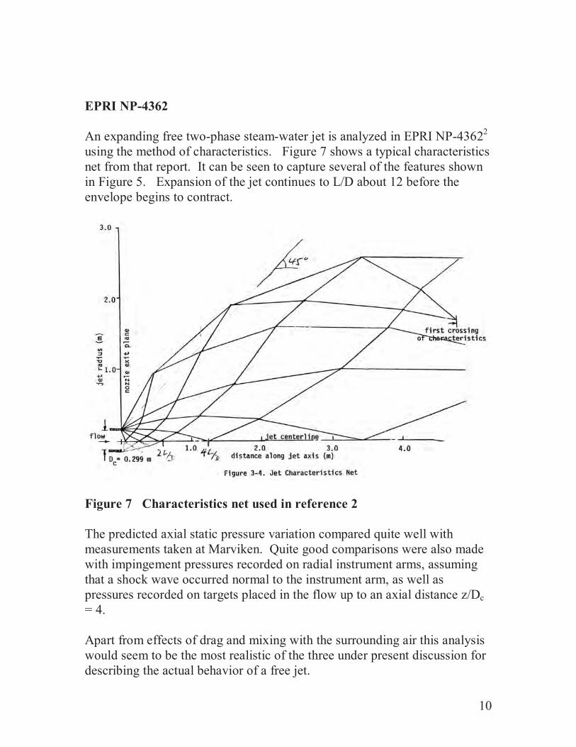
EPRI NP-4362 An expanding free two-phase steam-water jet is analyzed in EPRI NP-43622 using the method of characteristics. Figure 7 shows a typical characteristics net from that report. It can be seen to capture several of the features shown in Figure 5. Expansion of the jet continues to L/D about 12 before the envelope begins to contract.

Figure 7 Characteristics net used in reference 2 The predicted axial static pressure variation compared quite well with measurements taken at Marviken. Quite good comparisons were also made with impingement pressures recorded on radial instrument arms, assuming that a shock wave occurred normal to the instrument arm, as well as pressures recorded on targets placed in the flow up to an axial distance z/Dc = 4. Apart from effects of drag and mixing with the surrounding air this analysis would seem to be the most realistic of the three under present discussion for describing the actual behavior of a free jet.

11

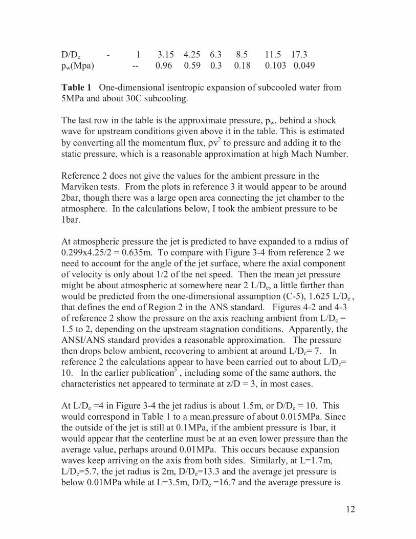
The flow is not one-dimensional. Unless there is mixing with the surrounding fluid, the surface of the jet is always at the ambient pressure and the conditions there are what would be predicted from isentropic expansion to ambient. They do not change along the jet. Therefore a small object placed just inside the jet boundary would experience exactly the same net force no matter where is was located relative to the nozzle. It is useful to compare the flow field with what would be predicted for one-dimensional isentropic expansion. In the Marviken test with p0 =5Mpa and a subcooling of 34C, the stagnation enthalpy is close to what would be obtained by starting with saturated water at 3Mpa, h=1008.4 KJ/kg, and compressing reversibly to 5MPa to add an additional enthalpy 2x103kPa x 0.0012m3/kg = 2.4kJ/kg to obtain h0=1010.8 kJ/kg. The stagnation entropy would still be the value for saturated water at 3Mpa, s0 = 2.6462kJ/kg.K. (These properties should be checked with tables for compressed water if greater accuracy is desired. The overall results below should not change much). The critical pressure ratio from may be estimated from Figure 3.2 in my book7 (this is for the Moody model but I assume it gives about the same critical pressure as the homogeneous model) as about 2/3 for saturated water at 3Mpa, namely 2Mpa. This ignores the overpressure at stagnation. The result is therefore approximate and predicts a lower choking pressure than in reference 4. From the usual isentropic relationships I computed the conditions at the nozzle exit to be a velocity of 106.8m/s and a density of 192.6kg/m3. It is not too important to get the choking pressure right if one is only interested in the calculation of flow areas. What matters is the flow per unit area at the nozzle, which is a maximum at choking and is insensitive to the assumed pressure. The conditions at a series of pressures downstream were then computed. Using the continuity relationship, (1) I could then compute D/De. These predictions are tabulated in Table 1. p(MPa) 5 2 0.2 0.1 0.04 0.02 0.01 0.004 v(m/s) 0 107 367 430 505 558 604 660 ρ kg/m3 - 193 5.65 2.65 1.026 0.51 0.256 0.104

12

D/De - 1 3.15 4.25 6.3 8.5 11.5 17.3 pw(Mpa) -- 0.96 0.59 0.3 0.18 0.103 0.049 Table 1 One-dimensional isentropic expansion of subcooled water from 5MPa and about 30C subcooling. The last row in the table is the approximate pressure, pw, behind a shock wave for upstream conditions given above it in the table. This is estimated by converting all the momentum flux, ρv2 to pressure and adding it to the static pressure, which is a reasonable approximation at high Mach Number. Reference 2 does not give the values for the ambient pressure in the Marviken tests. From the plots in reference 3 it would appear to be around 2bar, though there was a large open area connecting the jet chamber to the atmosphere. In the calculations below, I took the ambient pressure to be 1bar. At atmospheric pressure the jet is predicted to have expanded to a radius of 0.299x4.25/2 = 0.635m. To compare with Figure 3-4 from reference 2 we need to account for the angle of the jet surface, where the axial component of velocity is only about 1/2 of the net speed. Then the mean jet pressure might be about atmospheric at somewhere near 2 L/De, a little farther than would be predicted from the one-dimensional assumption (C-5), 1.625 L/De , that defines the end of Region 2 in the ANS standard. Figures 4-2 and 4-3 of reference 2 show the pressure on the axis reaching ambient from L/Dc = 1.5 to 2, depending on the upstream stagnation conditions. Apparently, the ANSI/ANS standard provides a reasonable approximation. The pressure then drops below ambient, recovering to ambient at around L/Dc= 7. In reference 2 the calculations appear to have been carried out to about L/Dc= 10. In the earlier publication3 , including some of the same authors, the characteristics net appeared to terminate at z/D = 3, in most cases. At L/De =4 in Figure 3-4 the jet radius is about 1.5m, or D/De = 10. This would correspond in Table 1 to a mean.pressure of about 0.015MPa. Since the outside of the jet is still at 0.1MPa, if the ambient pressure is 1bar, it would appear that the centerline must be at an even lower pressure than the average value, perhaps around 0.01MPa. This occurs because expansion waves keep arriving on the axis from both sides. Similarly, at L=1.7m, L/De=5.7, the jet radius is 2m, D/De=13.3 and the average jet pressure is below 0.01MPa while at L=3.5m, D/De =16.7 and the average pressure is

13

down to near 0.004MPa. Apparently, were this center streamline brought to rest, the pressure achieved would be sub-atmospheric on a small object. If the target were large, there would have to be a shock wave standing off far from the target in order to achieve a stagnation pressure greater than atmospheric and allow the impacted mixture to escape. Yet the outer layer of the jet still has the conditions pertinent to 0.1MPa and, if it were to hit a small object, would achieve a pressure of 0.59MPa, perhaps enough to cause damage. If the jet were unstable and wobbling this large pressure would be available over a larger area than just the surface of a stable steady jet. A one-dimensional model cannot represent these large variations in properties across the jet After a distance of 4m the jet begins to contract. Some of the characteristics cross, indicating the formation of shock waves. If these are weak, the jet will collapse to conditions resembling those close to the nozzle, in the absence of other dissipative effects, as compression waves reflected from the free surface recompress the fluid. Then the impact pressures on targets will increase with distance from the nozzle. However, it appears from Figures 5 and 7, that there will be a normal shock at about L/D = 16 which will limit further significant refocusing of the jet energy and momentum. It seems likely that suitable computer program, such as FLUENT, could model these phenomena. FLUENT has already been used to compute a series of shock diamonds in a supersonic jet used in a combustion application. Table 1 shows that, if the ambient pressure is atmospheric, the density of the mixture at the jet boundary is 2.65kg/m3. As this is not all that much more than the density of a normal atmospheric environment, 1.2kg/m3, it is likely that mixing and friction will have significant effects when the jet length of interest is several L/Des. FLUENT can also model this, though an appropriate turbulence model would have to be chosen to get accurate results. Absent any other explanation, it appears that the ANSI/ANS Standard recommends a 10 degree half-angle jet growth as a result of this mixing. This prediction ignores the strong forces tending to collapse the jet inward, as a result of the high level of overexpansion and very low static pressures on the axis. If I use the 45 degree assumption, (C-5), and Table 1, a static pressure of 0.1MPa occurs at L/D = 1.625 and the impact pressure is 0.59MPa.

14

0.04MPa occurs at L/D of 2.65 and the impact pressure is 0.3MPa. 0.02MPa occurs at L/D=5.25 and the impact pressure is 0.18MPa. From Figure 2-6 of reference 2, the impact pressures are higher than these in the subcooled regime, probably because of the persistence of the subcooled core. In the "saturated liquid regime", with an upstream stagnation pressure of 3MPa, the impact pressures are 1.14MPa at L/D =1.2; 0.48MPa at L/D =2 and 0.24MPa at L/D =4. These fit into the sequence calculated from Table 1. So, the approximate model described in reference 4 is not too bad in this particular example and can apparently be extended beyond the "asymptotic plane" to some extent. While the approximate model presented in reference 4 has received some confirmation from experimental data at low L/Ds, up to 4 or 5, I have not seen experimental data at large L/Ds. The emphasis of tests has been mostly on the very large forces and pressures encountered on large targets close to the break. Though supersonic effects probably persist to at least L/D ~10 and the jets may still be quite potent for greater distances (I note that the LANL knowledge base report8 describes damage from steam jets at L/D =25 and from air jets at L/Ds as large as 100!) I have not seen any thorough analysis of jet behavior in this "far field". The ANSI/ANS approach that all is over at an "asymptotic plane" at the end of Region 2, around L/D =1.5 or 2, does not seem to correspond to reality. Continued expansion at a half-angle of 10 degrees in Region 3 also appears to have no clear justification and may predict too low an impact pressure at high L/Ds. It would perhaps be desirable to make suitable CFD predictions, and compare with experimental results, for longer L/Ds than have been used so far. Confined and free jets Figure 1 shows pressure (static: I will use "pressure" with no adjective to describe the static or thermodynamic pressure) contours, or isobars, for a jet confined between two walls. Figure 7 shows the characteristics net for a free jet. Unfortunately, the only isobar shown (I believe that Vic has some for a similar problem) is the jet boundary, which is at atmospheric pressure. These two problems are quite different. This is shown clearly by the velocity vectors in Figure 2. The only region where the two flow fields are the same is in a small region close to the nozzle that is unaffected by waves

15

reflected from the jet boundary. Even the corner flow seems different, with the free jet breaking out at an angle of about 600 while the confined jet is attached to the wall. In both cases the flow is isentropic through out the whole region until the flow passes through a shock wave. Therefore the pressure, density and velocity are related by the usual one-dimensional isentropic relations in these regions. The simple model developed in reference 4 to represent the Marviken results at low L/D appears to draw on the confined jet results. This is the only source that I have found for a model that appears to resemble that used for the Region 2 model in the ANSI/ANS Standard. The model may be reasonable as an approximation for impingement pressures on a large flat plate close to the nozzle, but it appears to be a stretch to use it for a free jet. Jet Pressure The Standard uses a "jet pressure", Pj , without giving a definition. It first appears in (D-4) where the force on a target is given by Fjt = ∫PjdAt (D-4) For a large target that diverts all of the flow sideways perpendicular to the jet axis (an approximation) the net force is the same as the "jet blowdown force" give by (D-1) and (D-2), neglecting the ambient pressure, Fj=Fb=CTP0 Ae= Ge

2Ae/ρe +AePe =Ae(ρeve2 + Pe) (2)

A momentum balance for a free jet in the z-direction of the axis is Fj = Ae(ρeve

2 + Pe) = ∫ (ρvz2 + P – Pa) dAj (3)

This resembles (D-4) but it is not the same. Pj , the pressure on the plate, is a quite different animal from the pressure in a free jet or the maximum pressure which a free jet would exert on a small object in the flow. In Region 3 the jet is assumed to be all at ambient pressure and the velocity is approximately in the z-direction, so (3) reduces to

16

Fj = ∫ ρv2 dAj (4) Examining (D-12 ) and (D-13) we find that the "jet pressure" has been assumed to vary linearly with distance from the axis such that Pj = Pjc(1 – r/rj) (5) with the centerline "pressure" given by Fj = ∫ Pj dAj = (Pjc/3) Aj (6) Comparing with (4) it appears that Pj in this region is the same as the momentum flux, ρv2. Now, this is not the same as the stagnation pressure, or the maximum pressure when the flow is brought to rest against an object. For moderate subsonic velocities, the stagnation pressure exceeds the ambient pressure by 1/2 ρv2 so there appears to be an overestimation by a factor of two. Moreover, (6) shows that the peak "jet pressure" on the centerline is three times the average value. If there is little mixing with the surrounding air, the jet profile would probably be fairly flat, so the potential overestimate is a factor of six. Mixing with surrounding air at the same density as the jet (another limiting case) might produce the sort of velocity profile characteristic of a turbulent jet, shown in Figure 24.9 on page 749 of Schlichting's "Boundary Layer Theory", which might conceivably be shown to be approximated by (D-12). The actual degree of mixing would depend on the density of the containment atmosphere. In Regions 1 and 2 the formula for the "jet pressure" is more complicated but it has a radial dependency that brings it to zero at the outer boundary. For example, (D-9) has Pj varying as (1 – r/rj)2 and (D-10) has it proportional to (1-r/rj)(1-br/rj) where b is a further geometrical factor. These pressure distributions are quite different from those that actually occur in a real jet. As discussed earlier, in the absence of mixing there is a region where both the static pressure and the pressure behind a local shock wave attain maximum values on the outer boundary of the jet, a pattern that is the inverse of what is assumed. Even thought the radial pressure distribution may be wrongly modeled, there is some basis for using a "jet pressure". Comparing (D-4) and (3) the

17

pressure on a target may be equated to properties in the jet flow field if the jet pressure is defined as Pj = (ρvz

2 + P – Pa) (7) This will be the effective pressure difference between the front and back of the target if the pressure on the front is (ρvz

2 + P), which is an approximation to the pressure behind the shock wave shown in Figure 1 if the shock is almost parallel to the wall and is strong enough so that the velocity behind the shock can be neglected. This is what was done earlier in deriving pw in Table 1 and appears to be the basis of the simple model in reference 4. An Example I tried to follow the methods described in the standard for a special case of discharge from saturated conditions at 2000psia. Using the isentropic homogeneous equilibrium model, which tends to be valid for large pipe diameters, because the flow at the same velocity has a longer distance to travel to come to equilibrium, I deduced the values in Table 2. P(psia) 2000 1600 1400 1200 14.96 v(ft/s) 0 357 470 581 2422 ρ(lb/ft3) 23.1 17.7 13.45 0.0978 ρv(lb/ft2.s) 0 8246 8332 7816 241.9 P+ρv2(psi) 2000 2235 2245 Table 2 One-dimensional isentropic discharge from 2000psia, saturated water. The maximum mass flux occurs around 1400psia, close enough. The thrust coefficient is 2245/2000 = 1.125, which is low compared with 1.2 from figures B-3 and B-5 at stagnation pressures up to 1000psia and fL/D=0. Figure B-6 would appear to give a value closer to 1.17 at 2000psia. These values depend on the choked follow model. I am not too concerned with a difference of around 5%.

18

If the flow expanded entirely one-dimensionally, which appears to be the assumption in reference 4, the area at which atmospheric pressure would be achieved is given by the ratio of mass fluxes in Table 2 and is Aa/Ae = 8332/241.9 = 34.45 (8) The question now is how the authors of the standard achieved the value of around 85 for the same problem in the top figure C-4. One idea is that they used the overall momentum balance for the jet. When the pressure is atmospheric, it is simply, from (4) with a uniform velocity profile, Ft = CT P0Ae = Ae(ρeve

2 + Pe) = Aaρv2 (9) Putting in the numbers gives Aa/Ae = 2245 x 32.2 x144/2472/241.9 = 17.4 which is even further from the value in the standard. The reason for the discrepancy between (8) and (9) is that the momentum flux obtained for a jet in a nozzle that encloses the flow and extends from the hole in the pipe to the atmospheric plane exceeds the impulse (or jet force) from the break itself by the amount of impulse given by the force distribution on the nozzle walls. Then the momentum in the jet from a flow confined in the enclosed nozzle is about twice what it would be in the unconfined case. The only way to get twice the momentum from the same density and velocity is to have twice the area. It will then appear that conservation of mass is violated, since twice the area would give twice the flow. The answer lies in the velocity and pressure distribution across the jet, as well as the direction of the velocity vector, since only the z-component contributes to the z-direction momentum and mass transport. An enclosed flow in a nozzle may be made to be close to one-dimensional, so that the simple control volume methods work out quite well. The expansion from a hole is far from one-dimensional, with some of the velocity vectors at perhaps 600, typically, from the z-axis, contributing only one half of the mass flux and one quarter of the momentum flux in the z-direction that they would if they were pointed along the jet axis. The

19

pressure distribution across the jet is also far from uniform (the isobars follow the constant Mach Number contours in the part of the flow shown in Vic's report, before a shock is passed through). We may now try to manipulate (9) using the one-dimensional continuity equation (with all its approximations!), in the form already given in (1). The velocity va may be eliminated between (1) and (9) to get Aa/Ae = ve

2ρe2 /(ρaCTP0) (10)

which is the form used in the Standard as (C-3). Substituting the numbers gives Aa/Ae = (8332)2 / 32.2/0.0978/2245/144 = 68 (11) The factor of two that made (9) one half of (8) has now been inverted to make the predicted area now twice what was predicted by (8). It is the same "correction factor" for non-one-dimensional effects, but because of the manipulations, which involve squaring (1) and multiplying (9), it has been transferred form numerator to denominator. The point is that using overly simple one-dimensional flow concepts in a situation involving very strong two-dimensional effects can lead to substantial errors in either direction, depending on how the errors are made to combine. As far as I can make out, the area predicted by (9) is the one used in reference 4 and it differs form what is shown in Figure C-4 of the standard by a factor of 5. We still have not achieved the area ratio in Figure C-4. In order to do so we need to look carefully at the definition of the atmospheric plane density below (C-3). There, the quality of the steam/water mixture is said to be calculated at the pressure Pa and the stagnation enthalpy, which is the enthalpy that the fluid has in the reactor vessel and would be the value of the enthalpy if the flow were brought to rest at a stagnation point. Working this out for constant enthalpy expansion from 2000psia, saturated, to atmospheric pressure I got x= 0.5068 and a density ρa of 0.0736, compared with the corresponding isentropic values of x=0.381 and ρa = 0.0978. Using this value of density in (10) yielded an area ratio of 90. It appears that the framers of the Standard did indeed follow their own instructions in deriving that figure.

20

This makes no sense. The jet flow at the (supposed) "atmospheric plane" has a high velocity of over 2000ft/s and is anything but "at rest" where stagnation conditions would hold. The model has become confused between that of a free jet and that of an impinging jet. The same problem occurs in Figure 1-4 in the Appendix 1 to the SER where the sketch defies reality. To summarize: there are two difficulties in computing the conditions at the "asymptotic plane". The first is due to the inconsistent assumptions of one-dimensionality that can create an error of a factor of two either way in the effective flow area, depending on how the equations are combined. The extreme cases differ by a factor of 4. The second problem is the use of quite the wrong definition of the average density at this plane. The combined effect appears to be a factor of 5 between what I interpret to be the method in reference 4 and the one used in the Standard. This is all quite independent of the observation that the supersonic effects are not "over" as some "asymptotic plane", as clearly shown in Vic's nice sketches of jets in his report9. So, it is not a good concept, as well as being poorly computed. References 1, ANSI/ANS-58.2-1980 American National Standard: Design Basis for Protection of Light Water Nuclear Power Plants against the Effects of Postulated Pipe Rupture". 2. EPRI NP-4362 "Two-Phase Jet Modeling and Data Comparison" S.Levy Inc. Principal Investigators, J.M.Healzer, E.Elias, Project manager Avtar Singh. Final Report March 1986. 3. "Modeling Two-Phase Jet Flow" E.Elias, J.M Healzer, A.Singh, and F.J.Moody. ASME PVP-Volume 91 pp. 63-72, 1984 4. NUREG-CR-2913 "Two-Phase Jet Loads". G Weigand, S.L.Thompson and D.Tomasko. Sandia National Laboratories January 1983

21

5. Fundamentals of Gas Dynamics. Jerzy A Owczarek. International Textbook Co. 1964 6. Modern Compressible Flow. John D. Anderson. McGraw-Hill 1982 7. One-Dimensional Two-Phase Flow. Graham B. Wallis. McGraw-Hill 1969 8. NUREG /CR-6808 "Knowledge Base for the Effects of Debris on Pressurized Water Reactor Emergency Cooling Sump Performance". Los Alamos National Laboratory D.V. Rao Principal Investigator. February 2003. 9. Comments on GSI-191 Models for Debris Generation. Victor Ransom 9/14/2004 10. "Boundary Layer Theory", Hermann Schlichting. 7th edition. McGraw-Hill, 1979