the analytic hierarchy process –what it is and how it used

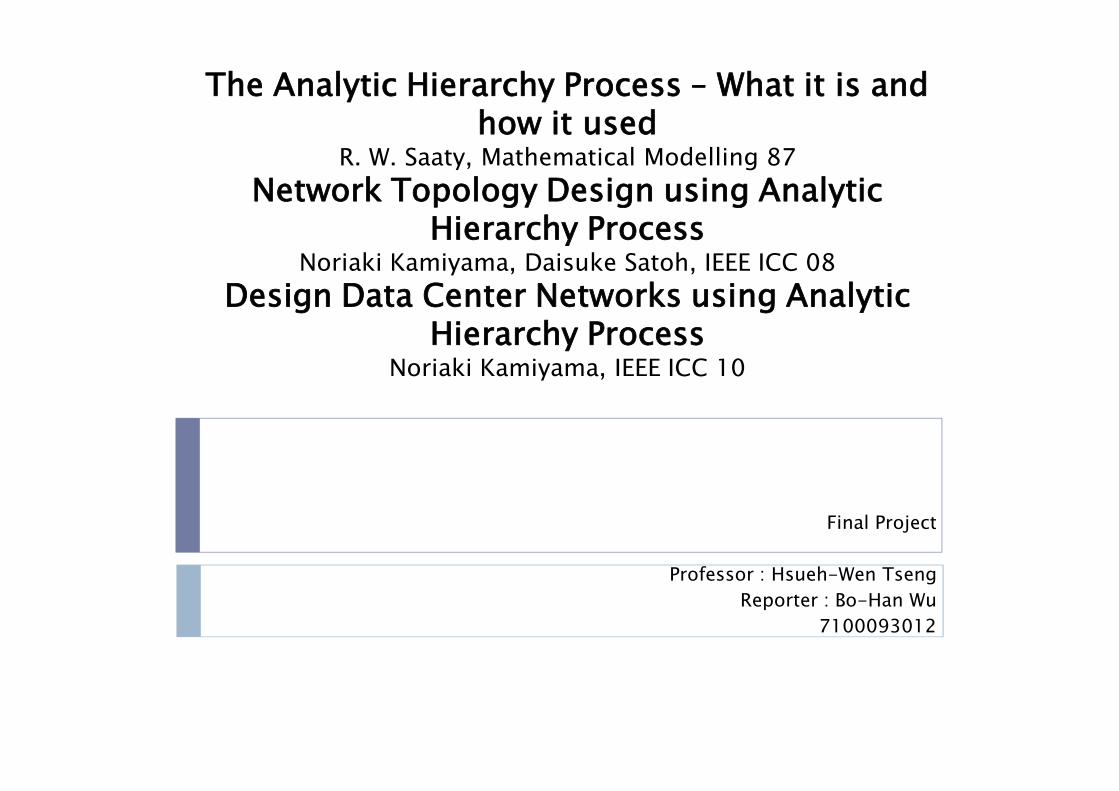
The Analytic Hierarchy Process – What it is and how it used

R. W. Saaty, Mathematical Modelling 87Network Topology Design using Analytic

Hierarchy ProcessNoriaki Kamiyama, Daisuke Satoh, IEEE ICC 08

Design Data Center Networks using Analytic Hierarchy Process

Noriaki Kamiyama, IEEE ICC 10

Final Project

Professor : Hsueh-Wen TsengReporter : Bo-Han Wu

7100093012

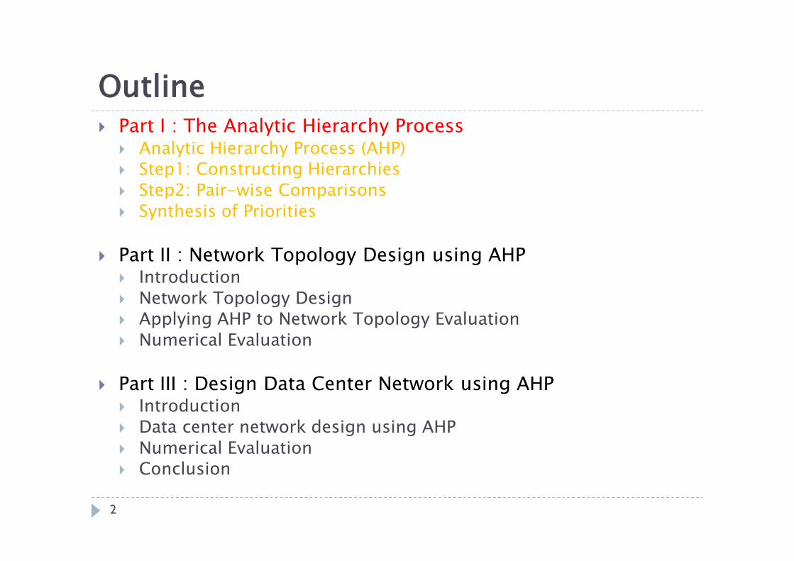
Outline Part I : The Analytic Hierarchy Process

Analytic Hierarchy Process (AHP) Step1: Constructing Hierarchies Step2: Pair-wise Comparisons Synthesis of Priorities

Part II : Network Topology Design using AHP Introduction Network Topology Design Applying AHP to Network Topology Evaluation Numerical Evaluation

Part III : Design Data Center Network using AHP Introduction Data center network design using AHP Numerical Evaluation Conclusion

2

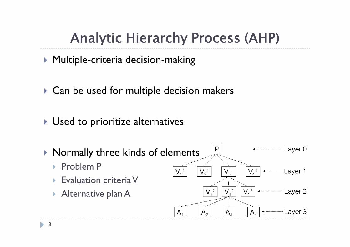
Analytic Hierarchy Process (AHP) Multiple-criteria decision-making

Can be used for multiple decision makers

Used to prioritize alternatives

Normally three kinds of elements Problem P Evaluation criteria V Alternative plan A

3

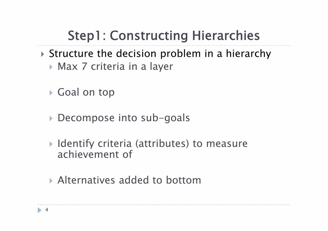
Step1: Constructing Hierarchies Structure the decision problem in a hierarchy Max 7 criteria in a layer

Goal on top

Decompose into sub-goals

Identify criteria (attributes) to measure achievement of

Alternatives added to bottom

4

Step1: Constructing Hierarchies (cont.)• Example :

5

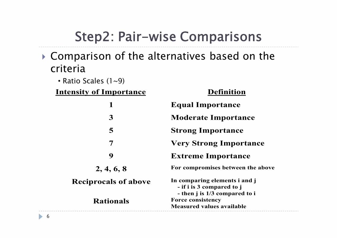
Step2: Pair-wise Comparisons Comparison of the alternatives based on the

criteria• Ratio Scales (1~9)

Intensity of Importance Definition

1 Equal Importance

3 Moderate Importance

5 Strong Importance

7 Very Strong Importance

9 Extreme Importance

2, 4, 6, 8 For compromises between the above

Reciprocals of above In comparing elements i and j - if i is 3 compared to j - then j is 1/3 compared to i

Rationals Force consistency Measured values available

6

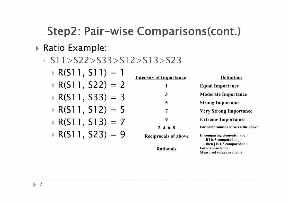
Step2: Pair-wise Comparisons(cont.) Ratio Example:

• S11>S22>S33>S12>S13>S23 R(S11, S11) = 1 R(S11, S22) = 2 R(S11, S33) = 3 R(S11, S12) = 5 R(S11, S13) = 7 R(S11, S23) = 9

Intensity of Importance Definition

1 Equal Importance

3 Moderate Importance

5 Strong Importance

7 Very Strong Importance

9 Extreme Importance

2, 4, 6, 8 For compromises between the above

Reciprocals of above In comparing elements i and j - if i is 3 compared to j - then j is 1/3 compared to i

Rationals Force consistency Measured values available

7

Step2:Pair-wise Comparisons (cont.) Judge Matrix: rij>0 rii=1 rji=1/rij

1/1/1

1/11

1

11

21

212

112

21

221

112

mm

m

m

mm

m

m

ij

rr

rrrr

rr

rrrr

rA

8

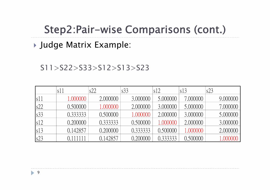
Judge Matrix Example:

S11>S22>S33>S12>S13>S23

s11 s22 s33 s12 s13 s23

s11 1.000000 2.000000 3.000000 5.000000 7.000000 9.000000

s22 0.500000 1.000000 2.000000 3.000000 5.000000 7.000000

s33 0.333333 0.500000 1.000000 2.000000 3.000000 5.000000

s12 0.200000 0.333333 0.500000 1.000000 2.000000 3.000000

s13 0.142857 0.200000 0.333333 0.500000 1.000000 2.000000

s23 0.111111 0.142857 0.200000 0.333333 0.500000 1.000000

Step2:Pair-wise Comparisons (cont.)

9

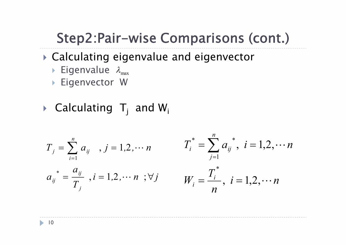
Step2:Pair-wise Comparisons (cont.) Calculating eigenvalue and eigenvector Eigenvalue Eigenvector W

Calculating Tj and Wi

max

jn,,iTa

a

n,,jaT

j

ijij

n

iijj

; 21,

21,

*

1

ninTW

niaT

ii

n

jiji

,2,1 ,

,2,1 ,

*

1

**

10

Example:• Judge Matrix

*ij n

TW ii

*

n

jiji aT

1

**

s11 s22 s33 s12 s13 s23

s11 1.0000 2.0000 3.0000 5.0000 7.0000 9.0000

s22 0.5000 1.0000 2.0000 3.0000 5.0000 7.0000

s33 0.3333 0.5000 1.0000 2.0000 3.0000 5.0000

s12 0.2000 0.3333 0.5000 1.0000 2.0000 3.0000

s13 0.1429 0.2000 0.3333 0.5000 1.0000 2.0000

s23 0.1111 0.1429 0.2000 0.3333 0.5000 1.0000

Tj(行和) 2.2873 4.1762 7.0333 11.8333 18.5000 27.0000

sij/Tj s11 s22 s33 s12 s13 s23 Ti Wi

s11 0.4372 0.4789 0.4265 0.4225 0.3784 0.3333 2.4769 0.4128

s22 0.2186 0.2395 0.2844 0.2535 0.2703 0.2593 1.5255 0.2542

s33 0.1457 0.1197 0.1422 0.1690 0.1622 0.1852 0.9240 0.1540

s12 0.0874 0.0798 0.0711 0.0845 0.1081 0.1111 0.5421 0.0903

s13 0.0625 0.0479 0.0474 0.0423 0.0541 0.0741 0.3281 0.0547

s23 0.0486 0.0342 0.0284 0.0282 0.0270 0.0370 0.2035 0.0339


11

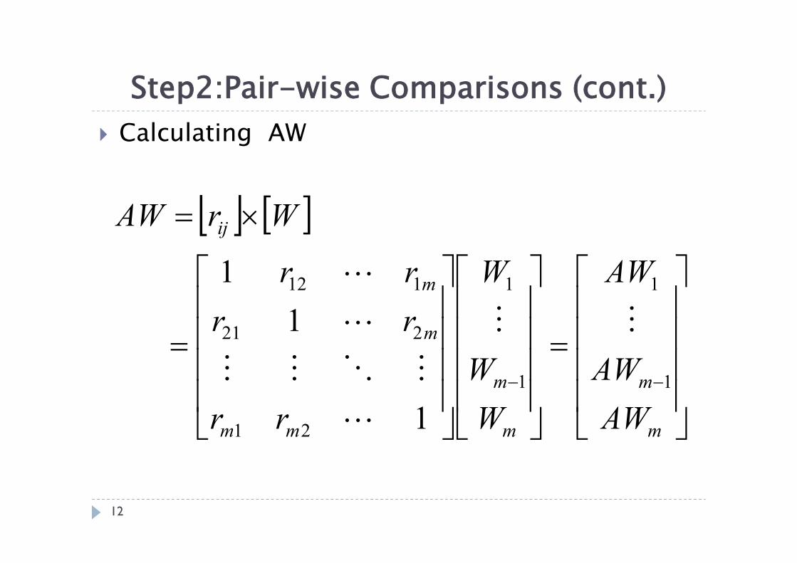
Calculating AW

m

m

m

m

mm

m

m

ij

AWAW

AW

WW

W

rr

rrrr

WrAW

1

1

1

1

21

221

112

1

11


12

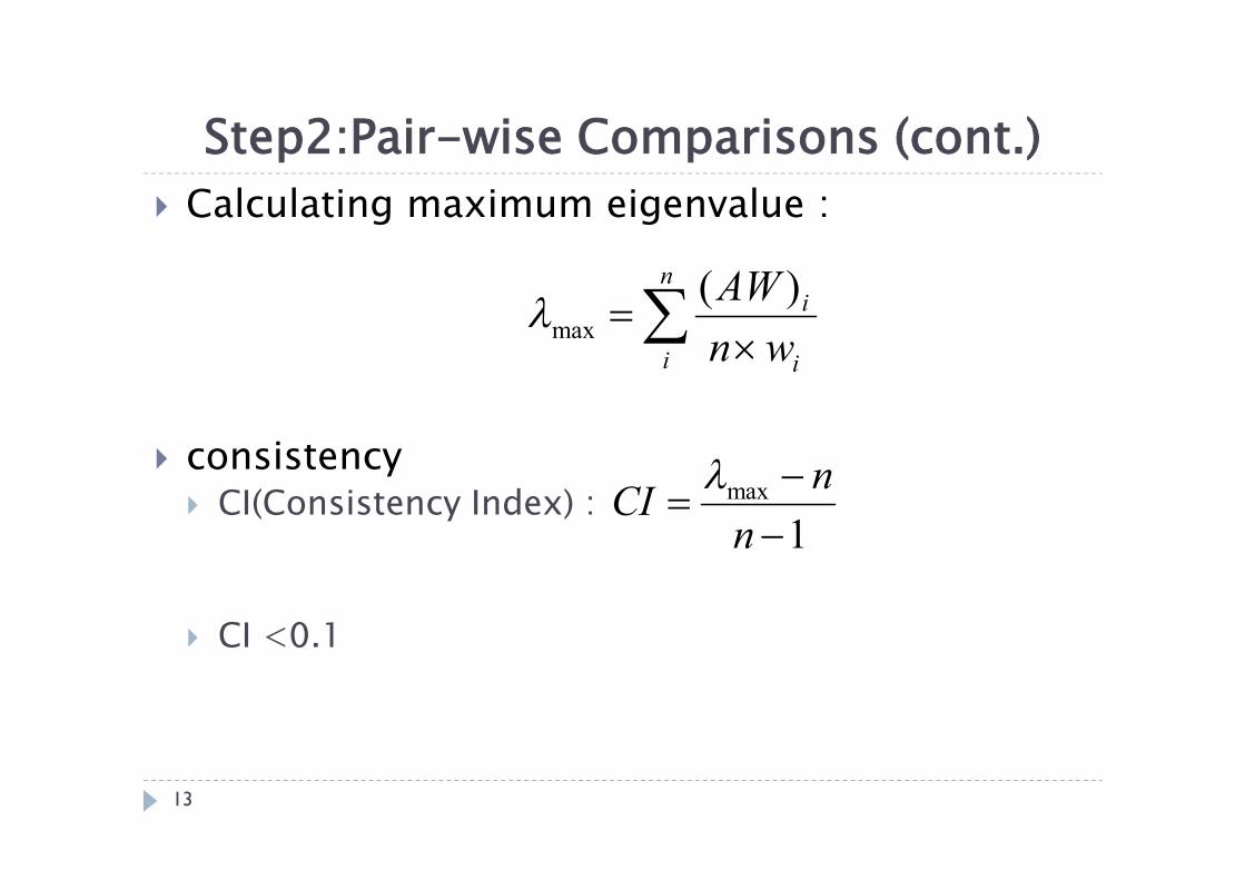
Calculating maximum eigenvalue :

consistency CI(Consistency Index) :

CI <0.1

n

i i

i

wnAW )(

max

1max

n

nCI


13

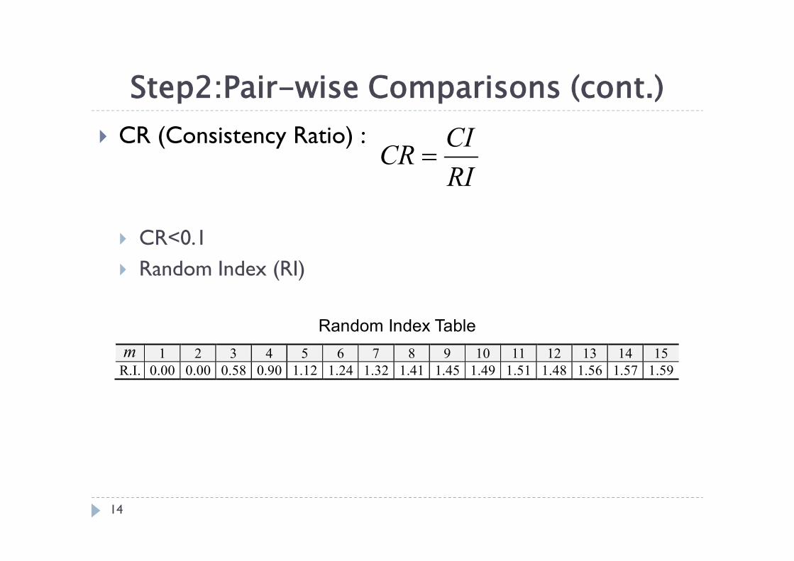
CR (Consistency Ratio) :

CR<0.1 Random Index (RI)

RICICR

Random Index Table m 1 2 3 4 5 6 7 8 9 10 11 12 13 14 15

R.I. 0.00 0.00 0.58 0.90 1.12 1.24 1.32 1.41 1.45 1.49 1.51 1.48 1.56 1.57 1.59


14

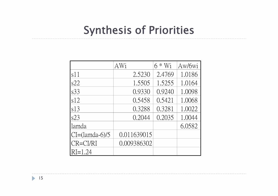
AWi 6 * Wi Aw/6wi

s11 2.5230 2.4769 1.0186

s22 1.5505 1.5255 1.0164

s33 0.9330 0.9240 1.0098

s12 0.5458 0.5421 1.0068

s13 0.3288 0.3281 1.0022

s23 0.2044 0.2035 1.0044

lamda 6.0582

CI=(lamda-6)/5 0.011639015

CR=CI/RI 0.009386302

RI=1.24

Synthesis of Priorities

15

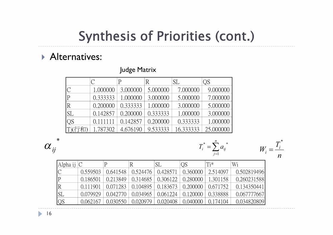
Alternatives:Judge Matrix

C P R SL QS

C 1.000000 3.000000 5.000000 7.000000 9.000000

P 0.333333 1.000000 3.000000 5.000000 7.000000

R 0.200000 0.333333 1.000000 3.000000 5.000000

SL 0.142857 0.200000 0.333333 1.000000 3.000000

QS 0.111111 0.142857 0.200000 0.333333 1.000000

Tj(行和) 1.787302 4.676190 9.533333 16.333333 25.000000

*ij

nTW i

i

*

n

jiji aT

1

**

Alpha ij C P R SL QS Ti* Wi

C 0.559503 0.641548 0.524476 0.428571 0.360000 2.514097 0.502819496

P 0.186501 0.213849 0.314685 0.306122 0.280000 1.301158 0.260231588

R 0.111901 0.071283 0.104895 0.183673 0.200000 0.671752 0.134350441

SL 0.079929 0.042770 0.034965 0.061224 0.120000 0.338888 0.067777667

QS 0.062167 0.030550 0.020979 0.020408 0.040000 0.174104 0.034820809

Synthesis of Priorities (cont.)

16

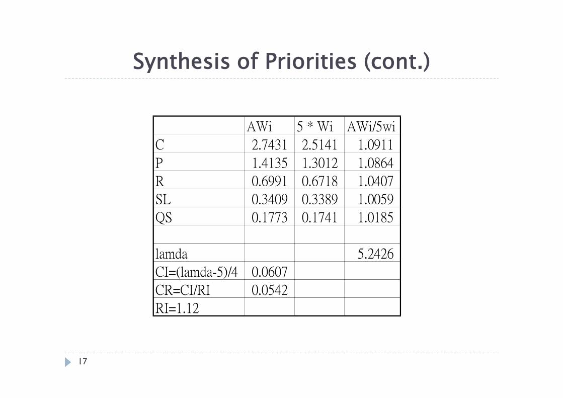
AWi 5 * Wi AWi/5wi

C 2.7431 2.5141 1.0911

P 1.4135 1.3012 1.0864

R 0.6991 0.6718 1.0407

SL 0.3409 0.3389 1.0059

QS 0.1773 0.1741 1.0185

lamda 5.2426

CI=(lamda-5)/4 0.0607

CR=CI/RI 0.0542

RI=1.12


17

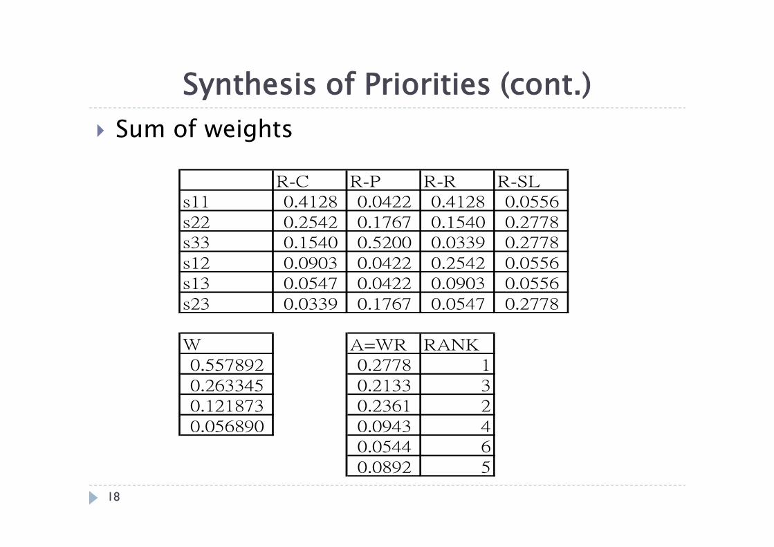
Sum of weights

R-C R-P R-R R-SL

s11 0.4128 0.0422 0.4128 0.0556

s22 0.2542 0.1767 0.1540 0.2778

s33 0.1540 0.5200 0.0339 0.2778

s12 0.0903 0.0422 0.2542 0.0556

s13 0.0547 0.0422 0.0903 0.0556

s23 0.0339 0.1767 0.0547 0.2778

W A=WR RANK

0.557892 0.2778 1

0.263345 0.2133 3

0.121873 0.2361 2

0.056890 0.0943 4

0.0544 6

0.0892 5


18





19

Introduction Network topology need to simultaneously

consider multiple criteria Cost Reliability Throughput …etc

Need to reflect the relative importance of each criterion when evaluating the network topology

This paper propose to use a linear-transformed value of each criterion when constructing weights in AHP

20

Network Topology Design Evaluation Criteria Total node count :

Total link length :

Sum of path lengths weighted by path traffic :

Amount of traffic on maximally loaded link :

21

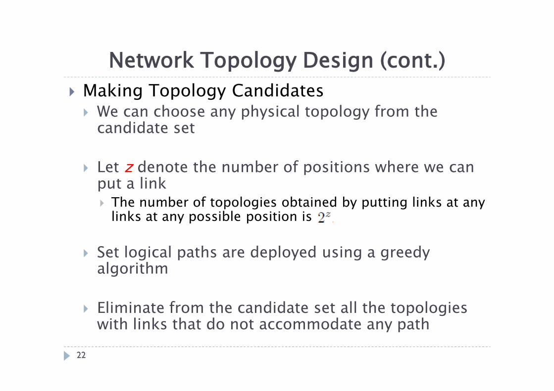
Making Topology Candidates We can choose any physical topology from the

candidate set

Let z denote the number of positions where we can put a link The number of topologies obtained by putting links at any

links at any possible position is

Set logical paths are deployed using a greedy algorithm

Eliminate from the candidate set all the topologies with links that do not accommodate any path

Network Topology Design (cont.)

22

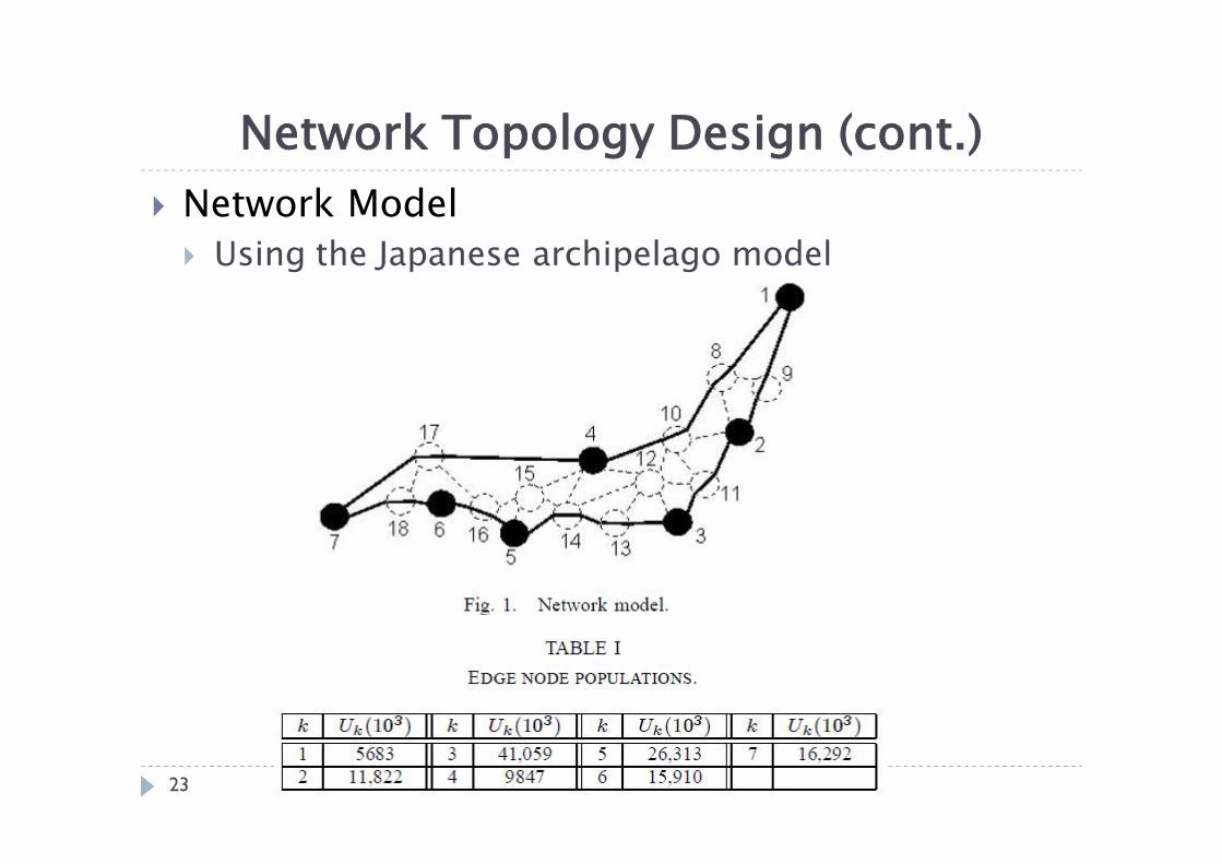
Network Model Using the Japanese archipelago model

Network Topology Design (cont.)

23

Applying AHP to Network Topology Evaluation

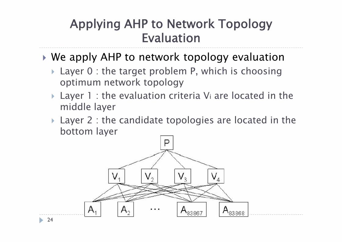
We apply AHP to network topology evaluation Layer 0 : the target problem P, which is choosing

optimum network topology Layer 1 : the evaluation criteria Vi are located in the

middle layer Layer 2 : the candidate topologies are located in the

bottom layer

24

Use the normalized value of , a linear-transformed value of

Define as a and b are arbitrary real numbers

Weights :

Applying AHP to Network Topology Evaluation (cont.)

25

Applying AHP to Network Topology Evaluation (cont.)

• Weights in descending order for each criterion

26

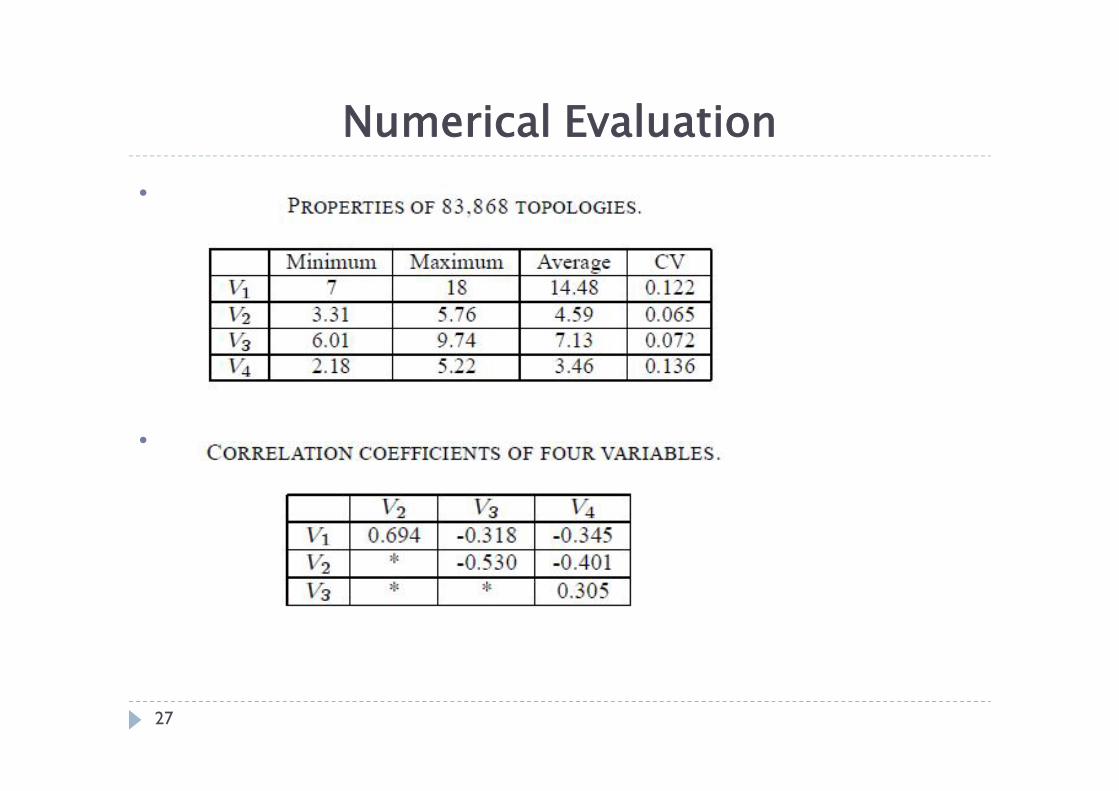
Numerical Evaluation•

•

27

• Example of scenarios for criteria comparisonNumerical Evaluation (cont.)

28

•

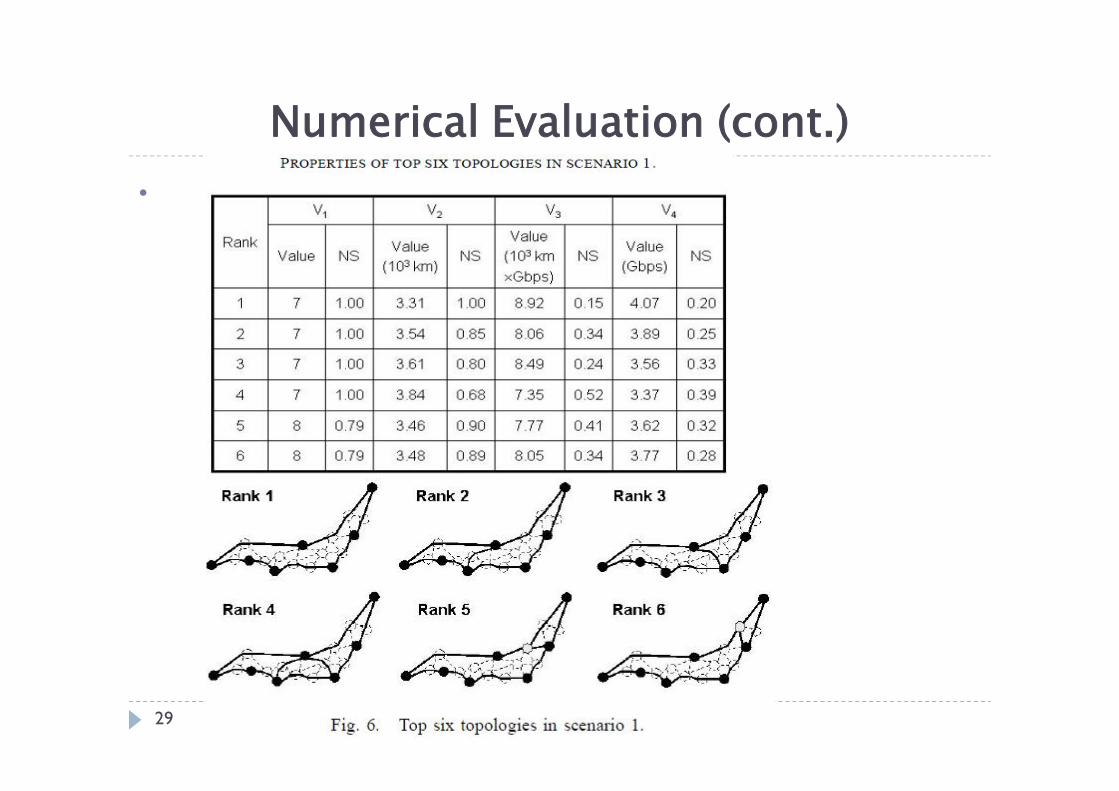
Numerical Evaluation (cont.)

29





30

Network topology and data center location strongly affect various evaluation criteria, such as cost, path length, and reliability

Design data center networks by evaluating both network topology and data locations simultaneously using AHP

Investigate the results of applying the proposed design method to three areas: Japan, USA, and Europe

Introduction

31

Data center network design using AHP Constructing candidate set of data center

network The constrains that all candidates need to satisfy are

To maintain the connectivity between all pairs of N nodes at any single link failure(SLF)

Have no links unused by traffic during normal operation as well as any SLF

Generate candidate data center network satisfying constraints The total number of candidates : N : nodes ; S : data center

32

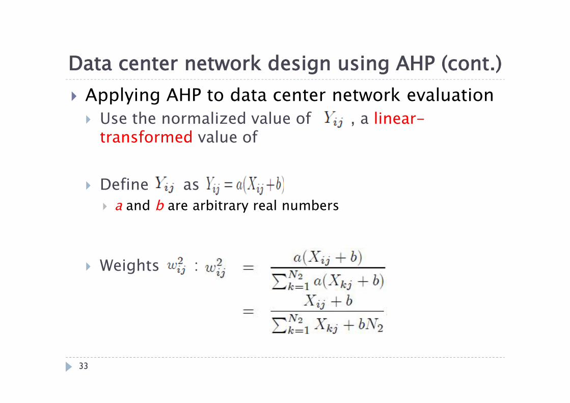
Applying AHP to data center network evaluation Use the normalized value of , a linear-

transformed value of

Define as a and b are arbitrary real numbers

Weights :

Data center network design using AHP (cont.)

33

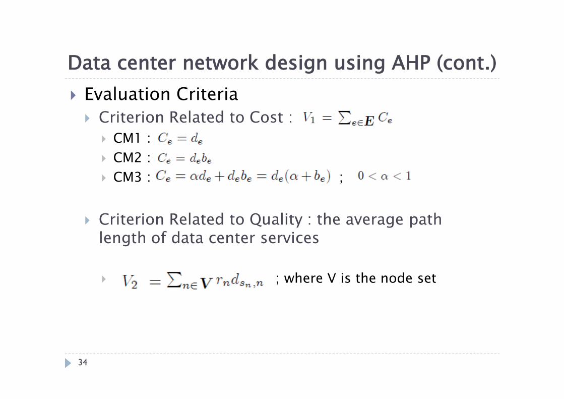
Evaluation Criteria Criterion Related to Cost :

CM1 : CM2 : CM3 : ;

Criterion Related to Quality : the average path length of data center services

; where V is the node set

Data center network design using AHP (cont.)

34

Numerical Evaluation • Node location and population

35

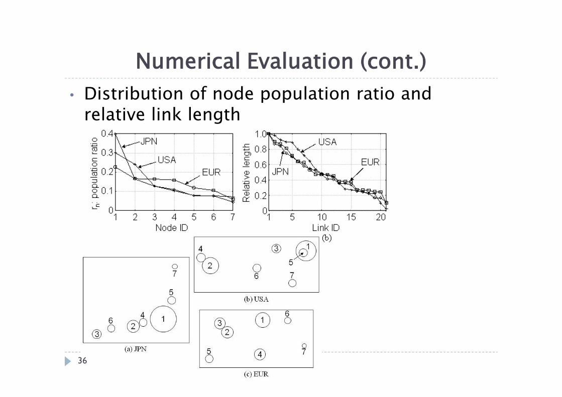
• Distribution of node population ratio and relative link length

Numerical Evaluation (cont.)

36

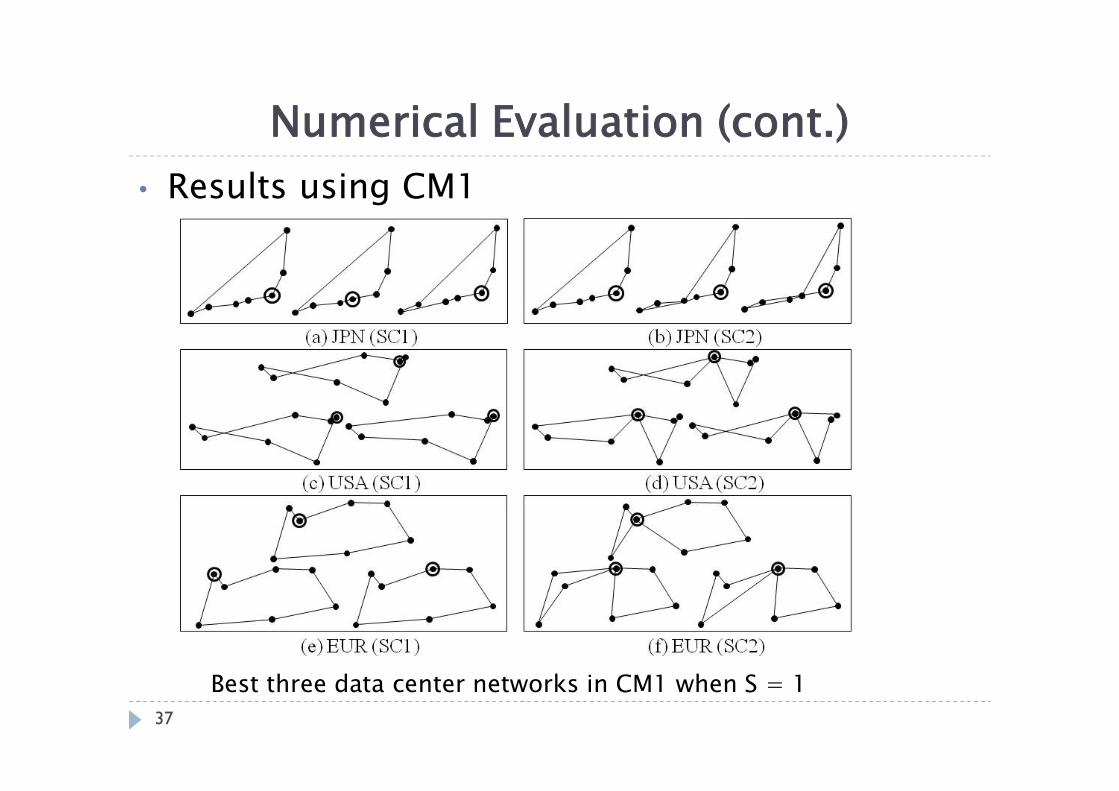
• Results using CM1Numerical Evaluation (cont.)

Best three data center networks in CM1 when S = 137

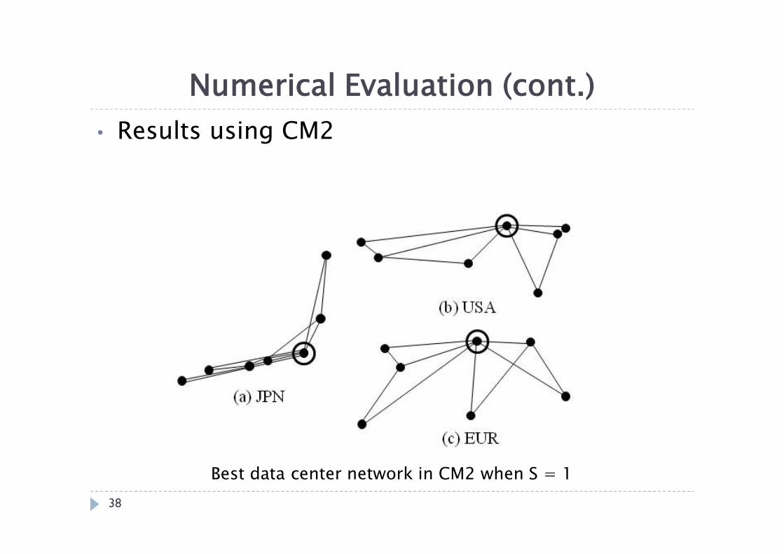
• Results using CM2Numerical Evaluation (cont.)

Best data center network in CM2 when S = 138

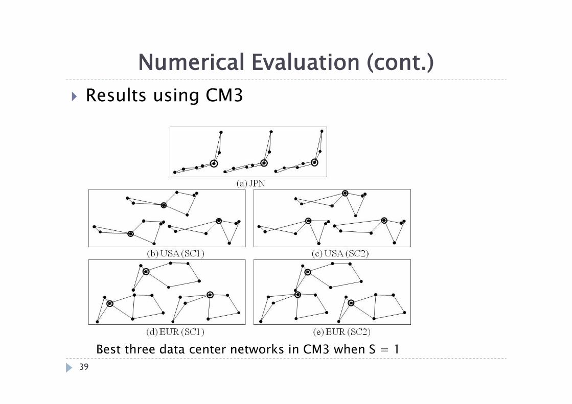
Results using CM3Numerical Evaluation (cont.)

Best three data center networks in CM3 when S = 139

Conclusion This paper presented a design method of data

center networks using AHP Generate candidates for data center networks

satisfying the requirements that connectivity between all pairs of nodes be maintained at single link failures (SLFs) and that no links are unused by traffic during normal operation and at any SLFs.

Evaluate the generated candidates by AHP using two criteria, i.e., the total link cost and the average path length

40

Question

41

Why use the AHP to design data center network ?• Ans :

Network topology and data center location strongly affect various evaluation criteria, such as cost, path length, and reliability; therefore, these criteria with different respective units need to be considered simultaneously when designing a data center network. The analytic hierarchy process (AHP) is a way to make a

rational decision considering multiple criteria.

the analytic hierarchy process –what it is and how it used

Documents