the analysis of change in differential psychology · differential psychology and indicators of...
TRANSCRIPT

The Analysis of Change in Differential Psychology Methodological Considerations, Skill-Acquisition and University Drop-Out
INAUGURALDISSERTATION
ZUR ERLANGUNG DES AKADEMISCHEN GRADES EINES DOKTORS DER
SOZIALWISSENSCHAFTEN
DER UNIVERSITÄT MANNHEIM
vorgelegt von
Dipl.-Psych. Manuel C. Völkle
Universität Mannheim
Fakultät für Sozialwissenschaften
Dezember 2007

Dekan der Fakultät für Sozialwissenschaften:
Prof. Dr. Josef Brüderl
Gutachter:
Prof. Dr. Werner W. Wittmann (University of Mannheim, Germany)
Prof. Dr. John R. Nesselroade (University of Virginia, USA)
Eingereicht am: 28.12.2007
Tag der mündlichen Prüfung am: 22.02.2008


I
PREFACE
In the present thesis the analysis of change is approached from the perspective of differential
psychology. Its goal is to strengthen, refine and extend the liaison between the methods of
differential psychology and indicators of change by comparing and integrating “conventional”
and “new” methods for the analysis of change, critically reviewing existing procedures, and
applying innovative new techniques to the analysis of practical problems.
Although the thesis is more comprehensive, and unique in its integration of various aspects of
change, different parts of it have already been published and/or presented before:
• Voelkle, M. C., & Sander, N. (in press). University drop-out: A structural equation
approach to discrete-time survival analysis. Journal of Individual Differences.
• Voelkle, M. C. (2007). Latent growth curve modeling as an integrative approach to the
analysis of change. Psychology Science, 49(4), 375-414
• Voelkle, M. C. (2007, April). Autoregressive latent trajectory models: A
reconsideration. Paper presented at the Annual Meeting of the American Educational
Research Association, Chicago.
Many people were involved in the completion of this thesis and I greatly appreciate their
many valuable suggestions, comments, and help with revising the manuscript. Above all,
however, I want to thank Prof. John R. Nesselroade for his willingness to serve as a reviewer.
My gratitude also goes to Dr. Nicolas Sander. Without him the fourth part of the thesis would
not have been possible. It was him who prepared the data and who provided me with
indispensable background information on the project. In a similar vein, I thank Prof. Phillip L.
Ackerman for allowing me – once again – to use his data on skill acquisition in TRACON to
illustrate my arguments in Section 3.
Special thanks go to ETS (Educational Testing Service) and my mentors at ETS for providing
me with such generous financial and academic support within the scope of the Harold
Gulliksen Psychometric Research Fellowship. The fourth part of the thesis was also
financially supported by the Karin-Islinger Stiftung. Academic training and some monetary
support was granted as part of the Quantitative Methods in the Social Sciences program of the
European Science Foundation.

II
Finally, the thesis in its present form is not least the result of the good cooperation, many
discussions, and great support of my dear colleagues and friends at the University of
Mannheim and around the world, who made writing this thesis an enjoyable undertaking. On
a more personal note, I want to thank Steffi Klingbeil for her appreciation of my work and her
patience with me during the less enjoyable days.
My primary acknowledgement, however, goes to my advisor and academic mentor Prof.
Werner W. Wittmann! Without him the present thesis would not have been possible. It is a
great honor to work with and learn from him and I am very obliged for his guidance and
unique support throughout all stages of my studies. Students of Prof. Werner W. Wittmann
will quickly recognize the “Dr. meth.” metaphor as the guiding principle underlying this
dissertation.
Mannheim, December 28th, 2007 Manuel C. Völkle

III
CONTENTS
1 INTRODUCTION ...............................................................................................................1
1.1 The analysis of change in differential psychology.......................................................2
1.1.1 A differential perspective ....................................................................................5 1.1.2 A structural equation modeling perspective .......................................................6
1.2 Statement of purpose ....................................................................................................9
1.3 Overview ....................................................................................................................10
2 LATENT GROWTH CURVE MODELING AS A GENERAL DATA-ANALYTIC SYSTEM FOR REPEATED MEASURES DESIGNS.............................12
2.1 Outline ........................................................................................................................15
2.2 Two-wave data ...........................................................................................................16
2.2.1 A latent growth curve approach to the analysis of two-wave data...................18 2.2.2 Change scores, residualized gain scores and latent difference scores.............20
2.3 Multi-wave data..........................................................................................................25
2.3.1 A latent growth curve approach to repeated measures ANOVA ......................25 2.3.2 Trend analysis...................................................................................................29 2.3.3 Overall significance tests and underlying assumptions....................................32 2.3.4 A latent growth curve approach to multivariate analysis of variance..............35 2.3.5 The latent growth curve modeling perspective .................................................37
2.4 Predicting change .......................................................................................................44
2.4.1 Predicting change in two-wave data.................................................................44 2.4.2 Predicting change in multi-wave data ..............................................................49 2.4.3 Extensions .........................................................................................................56
2.5 Discussion ..................................................................................................................58
3 A RECONSIDERATION OF AUTOREGRESSIVE LATENT TRAJECTORY (ALT) MODELS FOR THE ANALYSIS OF SKILL-ACQUISITION........................61
3.1 Outline ........................................................................................................................64
3.2 Nonlinear autoregressive latent trajectory models .....................................................65
3.3 An empirical example from the analysis of skill-acquisition.....................................68

IV
3.3.1 Linear LGCM....................................................................................................70 3.3.2 ALT-model.........................................................................................................71 3.3.3 Nonlinear LGCM ..............................................................................................74
3.4 A simulation study......................................................................................................75
3.4.1 Procedure..........................................................................................................75 3.4.2 Results .... ..........................................................................................................76
3.5 Discussion ..................................................................................................................81
4 A STRUCTURAL EQUATION APPROACH TO THE ANALYSIS OF UNIVERSITY DROP-OUT OVER TIME......................................................................83
4.1 Outline ........................................................................................................................86
4.2 Method........................................................................................................................86
4.2.1 A structural equation approach to discrete-time survival analysis ..................87 4.2.2 University drop-out over time...........................................................................96
4.3 Analysis and Results ..................................................................................................97
4.3.1 A discrete-time survival analysis of university drop-out ..................................97 4.3.2 Testing mediator effects in discrete-time survival analysis: The
relationship between high school GPA, university grade and university drop-out . .........................................................................................................101
4.3.3 The final model: Accounting for unobserved heterogeneity ...........................103 4.3.4 Limitations ......................................................................................................109
4.4 Discussion ................................................................................................................109
5 SUMMARY AND CONCLUSIONS ..............................................................................112
6 REFERENCES.................................................................................................................115
7 APPENDIX.......................................................................................................................130

V
LIST OF FIGURES
Figure 1 Framework for the analysis of change using SEM. The letters (a) to (e)
correspond to the five rationales for longitudinal research as proposed by
Baltes and Nesselroade (1979). ..........................................................................8
Figure 2 Path diagram of a paired samples t-test (A) and a base-free measure of
change model (B). The triangle represents the constant 1. Accordingly,
the two regression weights α0 and α1 are the means of the two latent
factors η0 and η1. φ represents their covariance and β10 the regression
weight of the regression of η1 on η0. The dotted error terms (ε1 and ε2)
indicate that the model does not account for measurement error
(mean(ε1) = mean(ε2) = sd(ε1) = sd(ε2) = 0). ....................................................19
Figure 3 Path diagram of a true change score model with two indicators (A) and a
base-free measure of change model with two indicators (B). The triangle
represents the constant 1. Accordingly, the two regression weights α0
and α1 are the means of the two latent factors η0 and η1. φ represents
their covariance and β10 the regression weight of the regression of η1 on
η0. ηt=1 is the true status at time point 1 and ηt=2 the true status at time
point 2. Other than in Figure 2, the variances of the error terms (ε1 and
ε2) are no longer constrained to zero. ...............................................................25
Figure 4 Path diagram and parameter estimates of a repeated measures
ANOVA/MANOVA.........................................................................................27
Figure 5 The same ANOVA/MANOVA model as shown in Figure 4 with all
means of the latent variables constrained to zero versus (//) freely
estimated. Intercepts (τ) of all manifest variables are fixed to zero. ................29
Figure 6 Saturated latent growth curve model with a factor loading matrix as
described in the text..........................................................................................38
Figure 7 Performance on a hypothetical learning task as introduced in Table 1.
The points along the dotted line indicate mean performance, as well as
the corresponding standard error, at each time point. The two solid lines
represent the trajectories of the best and worst individual at the last point

VI
of measurement. (A) Saturated (descriptive) model (B) estimated linear
model. ...............................................................................................................39
Figure 8 Linear latent growth curve model.....................................................................40
Figure 9 Quadratic latent growth curve model. ..............................................................42
Figure 10 Path diagram of a paired samples t-test (A) and a base-free measure of
change model (B) using either “sex” or “g” as predictor for individual
difference in pre- to posttest (x1 to x4) changes (sex // g). The predictor g
is z-standardized. Men are coded as 1 and women as 0. ..................................45
Figure 11 Multiple group analysis using gender as grouping variable. All freely
estimated parameters are allowed to differ across groups (saturated
model)...............................................................................................................48
Figure 12 Repeated measures (M)ANOVA with one between (sex) and one within
(time) subject factor, where only between-subject variance is predicted
by sex (no interaction between time and sex). Parameter estimates on the
right side of the graph are obtained when fixing the regression coefficient
of η0 on sex to zero (γ0sex = 0)...........................................................................50
Figure 13 Repeated measures (M)ANOVA with one between (sex) and one within
(time) subject factor. Interindividual differences in change over time are
predicted by sex (interaction between time and sex). Parameter estimates
on the right side of the graph are obtained when setting the regression
coefficients γ1sex = γ2sex = γ3sex = 0....................................................................52
Figure 14 Multiple group analysis using gender as grouping variable. All freely
estimated parameters shown in the path diagram are allowed to differ
between groups (saturated model). Parameter estimates on the left side of
the graph are obtained when all variances and covariances of the four
factors are constrained to equality, but the means are allowed to differ
across groups. Comparing the two models tests the assumption of
variance homogeneity.......................................................................................54
Figure 15 Quadratic LGC-model for the analysis of skill acquisition in TRACON
(solid lines). For the linear model β2 must be dropped. For the linear
ALT model the dotted lines are added, while the double lines have to be
removed (together with the quadratic growth factor in our example). For
VII
the sake of clarity, parameters have been omitted from the diagram. The
triangle at the top represents the constant 1. Its regression weights are the
means of the three latent factors and y1............................................................66
Figure 16 TRACON performance across six sessions. The points along the dotted
line indicate mean performance, as well as the corresponding standard
errors, at each session. Solid lines represent individual trajectories of the
5% best and 5% worst participants of the entire sample (at the sixth
session) and are intended to serve as an example of intraindividual
variation, as well as interindividual differences in intraindividual change
over time. Reprinted with permission from Voelkle, Wittmann &
Ackerman (2006)..............................................................................................70
Figure 17 Discrete-time survival analysis as a structural equation model with four
binary indicators and one predictor for k = 1 (solid lines). The number of
classes c can be easily increased (k > 1), taking unobserved
heterogeneity into account. The dotted lines illustrate further modeling
options such as the inclusion of additional predictors with time-varying
or time-invariant direct or indirect effects. More complex models can be
easily fit into this general SEM framework......................................................93
Figure 18 Estimated survival (solid line, left axis) and hazard (dashed line, right
axis) probabilities of university drop-out. ........................................................98
Figure 19 Three discrete-time survival models of university drop-out. A) Direct
effect of high school GPA or (symbolized by //) university grade on
drop-out. B) Direct and indirect effect (via university grade) of GPA on
drop-out (i.e. partial mediation). C) Completely mediated effect of high
school GPA (via university grade), on drop-out. All parameters are
significant unless otherwise noted. For a description of the model set-up
and discussion of parameter estimates the reader is referred to the text
and Footnote 29. .............................................................................................100

VIII
LIST OF TABLES
Table 1 Example data set of a hypothetical learning task with four repeated
points of measurement (x1 - x4) and two predictors (g and sex).......................17
Table 2 Repeated measures ANOVA. ...........................................................................27
Table 3 Independent samples t-test, repeated measures ANOVA and LGCM
approach to testing the difference in pre- to post-test improvement
between men and women. Note that (asymptotically) all three
approaches will yield identical results..............................................................46
Table 4 Model fit and parameter estimates of a linear LGC, linear ALT, and
quadratic LGC-model. ......................................................................................71
Table 5 Quadratic Latent Growth Curve (LGC) model. ...............................................77
Table 6 Linear Latent Growth Curve (LGC) model......................................................78
Table 7 Autoregressive Latent Trajectory (ALT) model...............................................79
Table 8 Person-Level and Person-Period data...............................................................88
Table 9 Life table...........................................................................................................90
Table 10 Descriptive statistics on the number of students in each cohort and at
each faculty, average university grade across all semesters, high school
GPA, and the number of students dropping out across the observation
period. ...............................................................................................................97
Table 11 Parameter estimates and model fit for a mediated DTSA, with and
without a direct effect of high school GPA on university drop-out as
described in the text........................................................................................101
Table 12 Parameter estimates and model fit of a three class discrete-time survival
mixture analysis..............................................................................................105

IX
ABBREVIATIONS
AIC = Akaike Information Criterion
ALT = Autoregressive Latent Trajectory
ANCOVA = Analysis of Covariance
ANOVA = Analysis of Variance
AR = Autoregressive
ARMA = Autoregressive Moving Average
ATC = Air Traffic Controller
BIC = Bayes Information Criterion
CFA = Confirmatory Factor Analysis
CFI = Comparative Fit Index
COR = Correlation
COV = Covariance
C.R. = Critical Ratio
DF = Degrees of Freedom
DTSA = Discrete-Time Survival Analysis
E( ) = Expected Value
G = General Intelligence
G-G = Greenhouse-Geisser
GPA = Grade Point Average
H-F = Huynh-Feldt
HLM = Hierarchical Linear Modeling
L = Likelihood
LGCM = Latent Growth Curve Modeling
LISREL = Linear Structural Relationships
LL = Log-Likelihood
LR = Likelihood Ratio
MA = Moving Average
MANOVA = Multivariate Analysis of Variance
MAR = Missing at Random
ML = Maximum Likelihood

X
MR = Multiple Regression
MS = Mean Squares
RMSEA = Root Mean Square Error of Approximation
SD = Standard Deviation
S.E. = Standard Error
SEM = Structural Equation Modeling
SRMR = Standardized Root Mean Square Residual
SS = Sum of Squares
TR( ) = Trace (of a matrix)
TRACON = Terminal Radar Approach Control
VAR = Variance

INTRODUCTION - 1 -
1 INTRODUCTION
“I want to take the risk and argue as forcefully as I can for some selective optimizing [of
research activities] by refocusing the targets to which the methods of differential psychology
are applied. The targets I wish to promote are selected indicators of change. This implies
paying less attention to applying the methods to single occasion scores” (Nesselroade, 2002,
p. 548).
The remarkably strong statement of John R. Nesselroade quoted above was taken from his
presidential address Elaborating the Differential in Differential Psychology given to the
Society of Multivariate Experimental Psychology, Saratoga Springs, NY, October 2000. In
his address he promotes a “liaison” (Nesselroade, 2002, p. 548) between the methods of
differential psychology and indicators of change and calls for a refinement, strengthening and
extension of this liaison. The guiding idea of the present thesis is to take up the call and
contribute to this goal by (a) comparing and integrating “conventional” and “new” methods
for the analysis of change, (b) critically reviewing existing procedures and (c) applying
innovative new techniques to the analysis of practical problems.
In line with Nesselroade (2002), the analysis of change will be approached from a differential
perspective, focusing on interindividual differences in intraindividual change over time. Per
definition this requires the analysis of intraindividual changes but also the analysis of
interindividual differences, which are independent of time but may be related to time-varying
characteristics.
Throughout the thesis a generalized latent variable perspective is adopted (Muthén, 2002).
Originally, structural equation modeling (SEM) was not developed for the analysis of
longitudinal data (e.g., Bollen, 1989), but it was soon discovered that it can easily be applied
to the analysis of change (Meredith & Tisak, 1984, 1990). Although various other techniques
exist for the analysis of longitudinal data, SEM is characterized by great flexibility, which
oftentimes permits the integration of other approaches as special cases, making it particularly
suited for the analysis of change.

INTRODUCTION - 2 -
Two studies serve as examples of the more general methodological considerations put
forward throughout the thesis. The first study (Section 3.3) is a reanalysis of data on skill-
acquisition in the complex problem solving scenario TRACON (Ackerman, Kanfer, & Goff,
1995). A latent growth curve analysis of skill-acquisition and its determinants (Voelkle,
Wittmann, & Ackerman, 2006) is used as a stepping stone towards a critical reconsideration
of the integration of autoregressive and latent growth curve models1. The second study
(Section 4) is a new study on university drop-out, thus methodological aspects and substantive
findings are considered to be of equal importance.
1.1 The analysis of change in differential psychology
As pointed out by Gottman (1995), “the study of change became the business of science” (p.
vii) ever since Galileo’s law of inertia overthrew Aristotle’s conception of a stable and
harmonic universe. Abandoning the idea that all objects have a natural place in universe, but
are in constant change, the analysis of things turns into the analysis of change of things. As a
consequence, methods for the analysis of change are as manifold as science itself. Although
they are unified in declaring change as their main object of investigation, there are great
differences of what constitutes change, or how to best analyze it. Accordingly, existing
methods are often closely bound to a particular discipline or sub-discipline, rendering any
comprehensive overview impossible. The spectrum ranges from the study of a single subject
assessed at comparatively few time points to the study of large samples repeatedly measured
on multiple variables over a long period of time. Typical examples are – but are not limited to
– the analysis of panel data (e.g., Wooldridge, 2007; Hsiao, 2005) and time series analysis
(e.g., Lütkepohl, 2005; Lütkepohl & Krätzig, 2004) in sociology and econometrics, latent
growth curve modeling (e.g., Bollen & Curran, 2006; Duncan, Duncan, & Strycker, 2006) and
hierarchical linear modeling (e.g., Raudenbush & Bryk, 2002) in the behavioral sciences and
closely related techniques in the health and medical sciences (e.g., Fitzmaurice, Laird, &
Ware, 2004), including the analysis of small sample or single subject designs (e.g., 1 The original latent growth curve study is already published and is explicitly not part of the present thesis. To
avoid any redundancies, the description of the theoretical background and the original analysis is kept to an
absolute minimum. For more detailed information the reader is referred to the Voelkle, Wittmann and Ackerman
(2006).

INTRODUCTION - 3 -
Kratochwill & Levin, 1992; Hoyle, 1999; Barlow & Hersen, 1984; Kazdin, 1982), models for
intensive longitudinal data (e.g., Walls & Schafer, 2006) and high-frequency data (e.g.,
Dacorogna et al., 2001) in such diverse areas as ambulatory assessment or the analysis of tick-
by-tick data in financial markets. Although there is an overlap in content and method among
the disciplines, different focuses and different terminologies make it difficult to see
commonalities or to transfer a procedure from one field of research to another. The same is
true for a universally valid definition of longitudinal research or a systematization of the
rationales and methods for the analysis of change. However, as pointed out by Baltes and
Nesselroade (1979), there is at least one common definitional criterion namely that “the entity
under investigation is observed repeatedly as it exists and evolves over time” (p. 4). While
Baltes and Nesselroade (1979) refer to longitudinal research, I prefer the more neutral term
analysis of change, but adopt the same conditio sine qua non for the analysis of change in the
present thesis2.
Five primary rationales for longitudinal research can be distinguished in the behavioral
sciences (Baltes & Nesselroade, 1979, p. 22ff.): a) the direct identification of intraindividual
change, b) the direct identification of interindividual differences in intraindividual change, c)
the analysis of interrelationships in (behavioral) change, d) the analysis of causes
(determinants) of intraindividual change and e) the analysis of causes (determinants) of
interindividual differences in intraindividual change. Practical examples and statistical
methods for all five rationales can be found in the present thesis, albeit some aspects are
emphasized more than others. Obviously, the first rational is a prerequisite for all subsequent
analyses and is inextricably tied to the assumption that the same entity is observed at least
2 The reason why I prefer the term “analysis of change” to “longitudinal analysis” is that the former explicitly
includes the analysis of two-wave data (i.e., change scores), which will be discussed in more detail in Section
1.2.2. As pointed out by Rogosa (1988; 1995), it is a “myth” that “two observations a longitudinal study make”
(1995, p. 8) so I think it would be better to reserve the term longitudinal for studies with at least three or more
time points. Although – technically speaking – two observations do a longitudinal study make, this notion
resulted in a number of misconceptions. However, because similar arguments can be raised against the use of
“analysis of change”, the two terms are used somewhat inconsistently. It is important, though, to note that two
time points are not sufficient to analyze the shape (i.e., curve) of change over time. In the words of Rogosa,
Brandt and Zimowski (1982): “two waves of data are better than one, but maybe not much better” (p. 744).

INTRODUCTION - 4 -
twice3. All methods treated in the following somehow deal with the identification of
individual change, although they differ in how this information is used. As will be discussed
at length in Section 2, traditional methods place great emphasis on mean changes, ignoring
much of the valuable information provided by individuals, while this information is of
primary interest for many of the more recently developed methods. The same is true for the
identification of interindividual differences in intraindividual change (b). If change over time
has been observed on an individual level, it becomes possible to describe differences between
entities. In growth curve modeling, a common way to capture these differences is to estimate
the variance of the individual growth rates (i.e., the linear and/or nonlinear slopes).
Subsequently, it becomes possible to analyze interrelationships in change (c). This can be
done with respect to different aspects of change in the same attribute, or with respect to
interrelationships in constancy and change between different attributes over time4. An
example of the former would be the correlation between a positive linear growth factor and a
negative quadratic growth factor, as described in more detail in Section 3. An example of the
latter would be parallel (multivariate) growth processes, which will not be discussed within
the context of this thesis (but see McArdle, 1989; MacCallum et al., 1997; Bollen & Curran,
2006). Once change over time can be described (a-c), it becomes possible to turn to the
prediction of change, either within the individual (d) or across individuals (e). The last two
aspects are often closely related. To illustrate this point, consider the analysis of university
drop-out, which will be discussed in Section 4. A student who fails all of his courses is
required to leave the university at some point in time. In other words, he changes his status
from being enrolled during a couple of semesters to the status of being no longer enrolled.
The determinant of this intraindividual change was the university grade. Similarly, one could
analyze the likelihood of dropping out (i.e., the hazard rate, see Section 4.2.1) over time and
relate this variable to university grade. The strength of the relationship indicates to which
3 As Baltes and Nesselroade (1979, p. 23f.) point out, if perfectly identical entities would have been exposed to
identical conditions across time, the cross-sectional methodology would be a true alternative to repeatedly
measuring the same entity. However, in the behavioral sciences this is a completely unrealistic assumption, so
that usually the “cross-sectional methodology is not a direct approach to the study of intraindividual change”
(Baltes & Nesselroade, 1979, p. 24). 4 This distinction is not made by Baltes and Nesselroade (1979).

INTRODUCTION - 5 -
degree interindividual differences in intraindividual change (i.e., in drop-out) are “caused” by
university grade (e).
1.1.1 A differential perspective
As already suggested by the title, the analysis of change is approached from the perspective of
differential psychology, thus it is the last aspect – the analysis of determinants of
interindividual differences in intraindividual change – which is of central interest in the
present thesis.
More than a century ago, Stern (1900; 1921, p. 15-19) laid the methodological foundations of
individual differences psychology by distinguishing between the analysis of the variation of a
single attribute across many individuals (Variationsforschung), the analysis of the correlation
between different attributes across many individuals (Korrelationsforschung), the analysis of
the variation across different attributes within a single person (Psychographie), and the
analysis of differences between two or more individuals across many attributes
(Komparationsforschung). His classification clearly dominated the first 50 years of research
in differential psychology and is still used today, with the vast majority of studies falling into
the second category of correlational research (Amelang & Bartussek, 1997, p. 31). However,
it is an implicit assumption of this classification that individuals do not change over time. This
was made explicit by Cattell (1957; 1966), who proposed a more general classification: the
ten dimensional basic data relation matrix (BDRM), better known in its simplified version,
the covariation chart (e.g., Cattell, 1980, p. 97ff.). The covariation chart explicitly contains
time (situations) as a third dimension, making it possible to account for potential changes. At
about the same time Cattell introduced his covariation chart and proposed different factor
analytic techniques to summarize the information contained in the three dimensions, first
statistical attempts were made to employ factor analysis to the organization of individual
growth curves (Tucker, 1958; Rao, 1958). From the perspective of differential psychology,
this was a major step forward, away from the analysis of mean changes towards the
estimation and prediction of individual trajectories. Since that time, two trends can be
observed. On the one hand, there is a steady improvement of statistical procedures to describe
and predict individual differences in change over time. Although the advancement was slow

INTRODUCTION - 6 -
at the beginning, there has been a great increase in research activities throughout the last
decade or two (see the next Section 1.1.2). However, at the same time this field of research
gains momentum, it appears to lose touch with traditional methods to analyze change over
time. As will be discussed in Section 2, this is unfortunate, because it creates a gap between
two research traditions which is not only counterproductive but also unnecessary (Cronbach,
1957, 1975). On the other hand, it appears to me that applied research does not keep pace with
many of the methodological advancements. Although there are more and more studies using
new methods for the analysis of change, even traditional strongholds in differential
psychology, such as research on learning or cognitive development, are lagging behind
methodological innovations.
1.1.2 A structural equation modeling perspective
The individual differences perspective is complemented by a methodological focus on
structural equation models (SEM)5. An overview of structural equation modeling is beyond
the scope of this thesis but is provided for example by Bollen (1989). The underlying
principles relevant for this thesis, however, will be recapitulated whenever necessary. I will
mainly adopt the traditional LISREL notation (Bollen, 1989, p. 10ff.), but will partially
deviate from this procedure across the three main parts of the thesis in order to improve
readability by being closer to the original literature. All changes in notation, however, are
clearly indicated.
Structural equation modeling is probably one of the prime examples of the possibilities that
can open up when targets to which the methods of differential psychology are applied are
refocused to indicators of change (see Nesselroade, 2002). As pointed out at the beginning,
originally SE-models were not developed for the analysis of change but were always closely
associated with differential psychology (Bollen, 1989; Bentler, 1980, 1986; see also
Hershberger, 2003; Wolfle, 2003). Tucker (1958) and Rao (1958) were the first who 5 Technically speaking, structural equation models are a special case of the more general latent variable models,
with standard latent growth curve models being a special case of structural equation models (e.g., Muthén,
2002). However, because the terms are treated fairly interchangeably in the literature, they are also used more or
less synonymously in the present thesis.

INTRODUCTION - 7 -
simultaneously – but independently of each other – proposed the application of factor analytic
techniques to the organization of individual growth curves. Early applications of their method
can be found in Scher, Young and Meredith (1960). Attempts to model individual growth
curves were made even earlier (Wishart, 1938; Robertson, 1908, 1909), a major breakthrough,
however, was the work of Meredith and Tisak (1990; 1984), who demonstrated how SEM can
be used to analyze change over time. This was the birth of latent growth curve modeling. A
more comprehensive review of the history of LGCM is provided for example by Bollen and
Curran (2006, p. 9ff.) or McArdle and Nesselroade (2002). Among others, it was primarily
McArdle (1986; 1988; 1989; 1991; McArdle & Epstein, 1987; McArdle & Hamagami, 1991,
1992) who advanced the original LGCM approach and applied it to a variety of
methodological and substantive problems. Especially during the last couple of years, the
original structural equation modeling approach – involving LGCM as a special case – has
been extended in many different directions, so that a complete overview is hardly possible and
certainly not reasonable for the purposes of the present thesis. A useful systematization,
however, was proposed by Muthén in his seminal article Beyond SEM: General Latent
Variable Modeling (2002; see also Muthén & Muthén, 1998-2007b; Muthén, 2001a; Muthén,
2001b; Muthén & Muthén, 2000). Based on his work, Figure 1 provides an overview of the
different modeling options made possible by second generation structural equation models
(Muthén, 2001b). Other than Muthén’s more general model (e.g., see Figure 1 in Muthén,
2002), Figure 1 has been particularly adopted to methods for the analysis of change, which are
of relevance to this thesis. For a description of the more general latent variable framework, the
reader is referred to the original literature.
Figure 1 is a pictorial representation of a system of simultaneous equations using standard
path diagram symbols (e.g., Bollen, 1989, p. 32ff.). Other than the path diagrams, which will
be employed later on, Figure 1 serves only the purpose of illustrating the various modeling
options and is not meant to represent a model, which could be estimated6. Squares represent
manifest variables and circles latent variables. Both can be continuous or categorical, as
indicated by the normal distribution, respectively the horizontal line, within some squares or
6 As a matter of fact, it is quite obvious that the model would not be identified (unless very specific constraints
are imposed).

INTRODUCTION - 8 -
circles. The four manifest variables represent the repeated measures at four time points, with
the two continuous latent variables representing different aspects of growth over time (e.g.,
linear or nonlinear change, or true interindividual differences at a given point in time, see
Section 2). The growth factors, as well as the repeated measures can be regressed on other
categorical or continuous observed variables as illustrated by the upper right square. In
addition, different classes of trajectories may be identified as illustrated by the categorical
latent variable (circle) in the upper left corner of Figure 1. Finally, the triangle represents the
constant 1 (actually a unit vector), so that the regression of any of the variables on 1
corresponds to the intercept of the regression equation. A more detailed description will be
provided in the course of the thesis.
Figure 1 Framework for the analysis of change using SEM. The letters (a) to (e) correspond
to the five rationales for longitudinal research as proposed by Baltes and Nesselroade (1979).
All five rationales for longitudinal research put forward by Baltes and Nesselroade (1979) are
contained in Figure 1. The individual (factor) scores of the two continuous latent variables
capture intraindividual change over time (a). Accordingly, their variance maps interindividual
differences in change (b). As indicated by the double-headed arrow between the two
continuous growth factors, different aspects of change can be interrelated (c). Determinants of
intraindividual changes (d) and interindividual differences in intraindividual change (e) may
be categorical or continuous and may either affect the growth factors or have a direct impact
e c
ab
ab
de
d e
1

INTRODUCTION - 9 -
on the manifest indicators. Without specific constraints, however, any direct impact would
only predict interindividual differences at a given point in time, but no changes. Finally, the
single-headed arrows connecting the observed variables represent an alternative way to model
change, which will be discussed in more detail in Section 3. Still other ways of modeling
change (e.g., full ARMA models, see Section 3) are possible, but only techniques, which will
be treated in this thesis, are contained in the Figure. It is obvious, that the present thesis is
somewhat selective with respect to the methods used for the analysis of change and the
emphasis that is put on certain aspects within these methods. However, as will be discussed
throughout the next four sections, these methods are often particularly suited for the analysis
of change from an individual differences perspective. But far be it from me to claim any
completeness of coverage of methods for the analysis of change in differential psychology.
1.2 Statement of purpose
The general purpose of the present thesis is to strengthen, refine and extend the liaison
between the methods of differential psychology and indicators of change as promoted by
Nesselroade (2002). As noted above (page 1), three attempts are made to contribute to achieve
this goal. Accordingly, the thesis is structured in three major parts. The purpose of the first
part is to bridge the gap between “traditional” and “new” methods for the analysis of change
by discussing latent growth curve models as a general data-analytic approach for repeated
measures designs. The purpose of the second part is to critically review a newly proposed
procedure (ALT-models) by pointing to problems in interpretation, which were not
considered before. Finally, the purpose of the last part is to highlight the advantages offered
by some recent developments in the analysis of change using categorical variables. A new
study of university drop-out serves as an example. With the present thesis it is hoped to
appeal to the methodologically interested reader and applied researcher alike. As a matter of
fact, the most general objective may be to strengthen the liaison between the development of
new methods and their use in applied research.
INTRODUCTION - 10 -
1.3 Overview
In the first part (Section 2) latent growth curve models are discussed as a general data-analytic
approach to the analysis of change. Conventional, but popular, methods of analyzing change
over time, such as the paired t-test, repeated measures ANOVA, or MANOVA, have a
tradition, which is quite different from the more recently developed latent growth curve
models. While the former originated from the idea of variance decomposition, the latter have
a factor analytic background. Accordingly, “traditional methods”, which focus on mean
changes, and “new methods”, with their emphasis on individual trajectories, are often treated
as two entirely different ways of analyzing change. In this section, an integrative perspective
is presented by demonstrating that the two approaches are essentially identical. More
precisely, it will be shown that the paired t-test, repeated measures ANOVA, and MANOVA
are all special cases of the more general latent growth curve approach. Model differences
reflect the underlying assumptions, and differences in results are a function of the degree to
which the assumptions are appropriate for a given set of data. Theoretical and practical
implications are set forth, and advantages of recognizing latent growth curve models as a
general data-analytic system for repeated measures designs are discussed.
After highlighting the versatility, generality and flexibility of the LGCM approach, the second
part (Section 3) takes a more critical stance on these alleged advantages and stresses the
importance of a good theory. In this section, a critical reconsideration of the recently proposed
simultaneous estimation of autoregressive (simplex) structures and latent trajectories (so
called Autoregressive Latent Trajectory (ALT) models, Bollen & Curran, 2004) is provided.
ALT models are becoming an increasingly popular approach to the analysis of change.
However, while historically autoregressive (AR) and latent growth curve models have been
developed independently from each other, the underlying pattern of change is often highly
similar. In this part it is argued that in practice, autoregressive (simplex) processes can be
inextricably confounded with nonlinear growth curve patterns. It is shown that an integration
of linear LGC- and AR-models can lead to severely biased parameter estimates. Accordingly,
researchers are cautioned that the combination of autoregressive and latent growth curve
models will often fail if the existence of nonlinear change cannot be ruled out. All arguments
are illustrated by empirical data on skill acquisition, and a simulation study is provided to

INTRODUCTION - 11 -
investigate the conditions and consequences of mistaking nonlinear growth curve patterns as
autoregressive processes.
While the first and second part are primarily of a theoretical nature, the third part (Section 4)
is concerned with the application of an innovative technique to the analysis of an important
practical problem: university drop-out. Accordingly, this part has a twofold purpose: Firstly, a
new approach to the analysis of change using categorical variables will be reviewed and,
secondly, a new study on university drop-out will be introduced. With increasing competition
among institutes of higher education regarding student selection, drop-out becomes a
politically and economically important factor for universities. While a number of studies
address this issue cross-sectionally by analyzing drop-out across different cohorts, or
retrospectively via questionnaires, few of them are truly longitudinal and focus on the
individual as the unit of interest (e.g., Gold & Kloft, 1991). In contrast to these studies, an
individual differences perspective is adopted in the present thesis. For this purpose, a hands-
on introduction to a recently proposed structural equation approach to discrete-time survival
analysis is provided (Muthén & Masyn, 2005). Particularly for the study of individual
differences, this technique is superior to traditional procedures. It not only permits an accurate
analysis of drop-out over time and its determinants, but also accounts for potential
heterogeneity among subjects. In a prospective study, N = 1096 students were observed across
four semesters. As expected, average university grade proved to be an important predictor of
future drop-out, while high school GPA yielded no incremental predictive validity but was
completely mediated by university grade. Accounting for unobserved heterogeneity, three
latent classes could be identified with differential predictor-criterion relations suggesting the
need to pay closer attention to the composition of the student population. An exploratory
analysis of a self-report measure as an additional predictor is provided and the findings are
discussed in the light of recent statistical advances and the current controversy about student
selection.

LGCM AS A GENERAL DATA-ANALYTIC SYSTEM - 12 -
2 LATENT GROWTH CURVE MODELING AS A GENERAL DATA-ANALYTIC
SYSTEM FOR REPEATED MEASURES DESIGNS
Almost forty years ago, Cohen (1968) showed that the analysis of variance (ANOVA) and
multiple regression analysis are essentially identical data analytic systems. His publication
received so much attention among social scientists like few other articles since that time. This
was even more surprising, given that the actual message was not new, and the underlying
mathematical principles were well known among statisticians. As a matter of fact, it was less
the ”discovery” itself, but more the theoretical and practical implications that came along with
it, which caught the attention of many researchers. A few years earlier, Cronbach (1957), in
his presidential address at the Sixty-Fifth Annual Convention of the American Psychological
Association, called for an integration of the “two disciplines of scientific psychology” (p.
671): Experimental and Correlational Psychology. Even though the distinction between the
two disciplines alludes to more than the use of different statistical procedures, the focus on
individual differences made regression techniques particularly interesting to correlational
psychologists. Experimental researchers, on the other hand, were typically more interested in
group differences, thus preferring the analysis of variance. By demonstrating that ANOVA
and multiple regression (MR) yield the same results if group membership is coded as a set of
dummy variables in MR, Cohen (1968) provided the methodological basis for an integration
of the two disciplines. Today, this is common knowledge among social researchers, even
though some introductory statistics texts still treat multiple regression and ANOVA as if these
were two completely unrelated techniques. Although not new in statistical content, Cohen’s
work (Cohen et al., 2003; Cohen & Cohen, 1983; Cohen, 1968) had a tremendous impact on
the statistical thinking of many researchers. On the one hand, it showed experimental
researchers the limits of the analysis of variance and exemplified the strict assumptions which
are associated with these models. To cite just one example, it is quite difficult to examine the
joint impact of a continuous and a categorical variable on a (continuous) dependent variable
within the framework of the analysis of variance. While the analysis of covariance
(ANCOVA) allows to adjust for a continuous covariate, it assumes that the regression slopes
are identical across all levels of the independent variable(s). This assumption corresponds to
an interaction of a categorical and continuous predictor, which could be easily tested within

LGCM AS A GENERAL DATA-ANALYTIC SYSTEM - 13 -
the multiple regression framework (Cohen, 1968, p. 439). On the other hand, it demonstrated
the flexibility of multiple regression, while at the same time pointing correlational researchers
to the dangers of this flexibility by comparing it to traditional ANOVA techniques. Referring
to the example above, probing the interaction between a single four category variable and a
continuous predictor would require the inclusion of three additional regression terms (e.g.,
Aiken & West, 1991). Although statistically possible and sometimes meaningful, one must
take great care to safeguard against alpha inflation, loss of power, or the interpretation of
practically irrelevant effects. Finally, however, Cohen’s work helped to integrate two different
ways of statistical thinking. The analysis of group differences and individual differences were
no longer viewed as fundamentally different research approaches in need of different
statistical procedures, but were shown to be closely related. As a result, researchers not only
gained a better understanding of the strengths and weaknesses of their preferred statistical
approach, but psychological research in general moved towards a fusion of its two disciplines
(Cronbach, 1975; Cook & Campbell, 1979).
Today, we find a similar situation in the analysis of change. On the one hand, there are the
“traditional approaches” dealing with the analysis of mean changes, on the other hand there
are the “new methods for the analysis of change” (Collins & Sayer, 2001) focusing on
individual changes over time. Both classes comprise an entire family of different models, with
the repeated measures ANOVA and Latent Growth Curve Models (LGCM) being the two
most prominent representatives of either class.
The ANOVA for repeated measures was developed as a direct extension of the fixed-effects
techniques of the analysis of variance pioneered by Fisher in the 1920s and ‘30s (e.g., Fisher,
1925). As shown in Equation (1), the basic idea is to partition the total sum of squares (SSTotal)
into one part which is caused by interindividual differences (SSBetween) and one part that is due
to intraindividual changes over time (SSWithin). Below I will come back to Equation (1), for
now it suffices to recall that this allows us to control for systematic but often unwanted
between-subject variance.
(1)BetweenWithinTotal SSSSSS +=

LGCM AS A GENERAL DATA-ANALYTIC SYSTEM - 14 -
What is not apparent from Equation (1) is the fact that this approach depends on a number of
strict assumptions. As a matter of fact, the underlying assumptions are often so unrealistic that
they are hardly ever met in practice. As a consequence, alternative procedures, such as the
multivariate analysis of variance (MANOVA), have been proposed for analyzing repeated
measures. Although less restrictive, MANOVA is a direct extension of the analysis of
variance and rests upon the same underlying idea of variance decomposition. Central to both
approaches is their focus on group changes instead of individual changes. The separation of
between- and within-subject variance is merely a means to the end of controlling for
differences between subjects in order to partition the remaining within-subject variance into
variation due to potential covariates (SSA) and variance not accounted for (SSError). As shown
in Equation (2), only group mean differences )( •− xxt for time point t = 1…T are of interest,
while all person (i = 1…N) specific deviations are treated as error variance.
(2)
As will be discussed below, this approach is often not only overly restrictive, but also ignores
valuable information contained in the data.
While interindividual differences in intraindividual change are treated as error variance in
traditional methods, they are of primary interest in latent growth curve modeling. As
discussed in Section 1.1.2 it was Meredith and Tisak (1990; 1984), who demonstrated that
SEM can be used to analyze longitudinal data. Using a slightly different notation, they
showed that individual change over time can be expressed as a structural equation
measurement model (Equation (3)), while interindividual differences in intraindividual change
correspond to the latent variable structural model (Equation (4)). The T repeated points of
measurement are represented by the T × 1 vector x. Accordingly, τ is a T × 1 vector of
intercepts and ε a T × 1 vector of person and time point specific error terms. η is an m × 1
vector of (growth) factors with the T × m factor loadings matrix Λ. As illustrated in Equation
(4), the latent factor(s) can be regressed on other exogenous or endogenous variables
(represented by the n × 1 vector ξ, respectively η) weighted by the m × n matrix Γ,
respectively the m × m matrix Β. Analogous to Equation (3), α is an m × 1 vector of intercepts
ErrorAWithin SSSSSS +=
∑=
•−=T
ttA xxNSS
1
2)(
and ∑∑= =
•+−−=N
i
T
ttitiError xxxxSS
1 1
2)(

LGCM AS A GENERAL DATA-ANALYTIC SYSTEM - 15 -
and ζ an m × 1 vector containing the error terms. Equations (3) and (4) will be discussed in
more detail further below. The resulting approach to the analysis of change is very general,
and as noted by Meredith and Tisak (1990) “with imagination and careful attention to detail,
given suitable identification, every form of repeated measures ANOVA or MANOVA can be
built up as a special case” (p. 114).
(3)
(4)
By demonstrating how to use common methods of covariance structure analysis to analyze
individual growth curves, they prepared the ground for present-day latent growth curve
models. Even though the technique has been extended during the last decade, the
mathematical basis is still the same. With some exaggeration, one could even say that there
are little advancements that were not envisioned in the original Meredith and Tisak (1990)
paper. This also applies to this first part of the thesis, where no large claim of originality is
being made. As a matter of fact, most of the material presented herein has already been
published in some scattered articles or chapters. However, I am not aware of any systematic
discussion of the conditions and consequences of integrating traditional analysis of variance
techniques into a general LGC-modeling framework. Typically, “traditional” methods to
analyze change and latent growth curve models are discussed separately, thereby emphasizing
their differences instead of their commonalities. In my view, however, much can be learned
about either approach by taking a closer look at their interrelationship. Latent growth curve
modeling must not be viewed as just another “tool in the toolbox of methods” but should be
understood as a very general data analytic system for repeated measures designs, which
incorporates paired t-tests, repeated measures ANOVA, and MANOVA as special cases. It is
hoped that the present thesis will help to evoke a similar “new look” (Cohen & Cohen, 1983,
preface) on the analysis of change as Cohen’s (1968) seminal article on multiple
regression/correlation analysis forty years ago.
2.1 Outline
This first major part of the thesis (i.e., Section 2) has three subsections and a concluding
discussion. In the first section (Section 2.2) I begin with the analysis of two-wave data and
εΛητx ++=
ζΒηΓξαη +++=
LGCM AS A GENERAL DATA-ANALYTIC SYSTEM - 16 -
demonstrate how the paired samples t-test can be viewed as a special case of a latent growth
curve model. Emphasis will be put on conceptual differences between change scores,
residualized (true) gain scores and latent difference scores. In Section 2.3, the discussion is
extended to multi-wave data by contrasting repeated measures ANOVA, MANOVA and
LGCM. The underlying assumptions of each approach will be highlighted and advantages of
LGCM to analyze change will be discussed. Section 2.4 deals with different ways to predict
change and provides a comparison across methods. I conclude with a discussion of the
theoretical and practical implications of latent growth curve modeling as a general data
analytic system.
2.2 Two-wave data
Two repeated points of measurement are the minimum requirement for the analysis of change.
Although two time points do not constitute a real longitudinal study (Rogosa et al., 1982;
Singer & Willett, 2003), the simple pre-post-test is probably one of the most often used
research designs in experimental research (but see Footnote 2). For example, one might be
interested in the effectiveness of an intervention, or improvement on a learning task, where
the performance of each individual has been assessed at the beginning and at the end.
Table 1 shows the scores of N = 17 female and N = 18 male participants on a hypothetical
learning task, where performance has been assessed on four consecutive time points (x1 to x4).
The data will be used to illustrate the main arguments throughout the remainder of this
section. Each score might correspond to the average number of points obtained and points lost
in a computer based complex problem solving scenario. Typical examples of such tasks are
TRACON or ATC (e.g., Ackerman, 1992; Ackerman & Kanfer, 1993). However, because the
data were chosen only for illustrative purposes, the reader is welcome to think of any other
(learning) task.

LGCM AS A GENERAL DATA-ANALYTIC SYSTEM - 17 -
Table 1 Example data set of a hypothetical learning task with four repeated points of
measurement (x1 - x4) and two predictors (g and sex).
Subject x1 x2 x3 x4 g sex 1 2.28 2.28 2.81 4.49 97.32 M 2 0.12 2.26 2.94 5.42 99.95 M 3 0.46 1.47 1.63 2.95 88.71 F 4 0.52 2.03 2.76 3.69 94.31 F 5 0.01 1.72 3.08 3.56 93.76 F 6 0.11 1.98 3.71 6.94 119.01 M 7 1.10 2.19 2.21 5.00 95.31 F 8 0.77 2.03 2.91 4.33 99.51 F 9 1.06 1.64 1.94 1.97 84.48 F 10 2.85 2.57 3.13 4.85 94.19 M 11 1.28 2.54 2.59 3.18 96.29 F 12 2.36 3.58 6.28 8.15 95.76 M 13 2.15 3.84 4.26 6.34 111.21 M 14 1.04 2.57 3.15 3.00 104.6 F 15 1.70 3.52 5.24 5.85 99.82 M 16 1.14 1.53 2.55 2.45 109.44 F 17 0.45 2.12 1.71 4.41 99.83 F 18 0.75 2.28 3.83 4.20 94.98 M 19 0.44 2.79 5.35 5.77 105.06 M 20 1.68 3.12 4.21 5.51 87.19 M 21 1.93 3.22 4.08 5.40 110.82 M 22 1.15 1.75 1.83 1.36 87.71 F 23 1.85 2.82 3.97 5.09 101.72 M 24 0.38 0.85 2.86 3.14 98.57 F 25 1.90 2.56 3.28 3.75 108.68 M 26 0.91 1.91 3.00 5.67 87.62 M 27 1.72 2.75 3.70 5.24 100.65 F 28 0.82 2.88 4.20 5.09 102.93 M 29 0.37 2.00 3.38 5.00 103.51 F 30 0.82 2.44 2.18 5.22 97.84 F 31 0.73 1.84 2.45 4.38 102.03 F 32 1.54 2.91 4.38 5.07 105.19 M 33 1.03 2.97 4.83 6.07 110.35 M 34 0.60 2.69 3.54 4.84 119.71 M 35 0.89 2.51 3.81 5.73 100.3 F Mean 1.11 2.41 3.37 4.66 100.24 SD 0.71 0.65 1.08 1.40 8.40
Total: covariances (correlations) x1 x2 x3 x4
x1 0.500 (1.00)
x2 0.274 (.601)
0.418 (1.00)
x3 0.259 (.339)
0.525 (.754)
1.162 (1.00)
x4 0.222 (.224)
0.604 (.666)
1.111 (.734)
1.971 (1.00)
Women: covariances (correlations) x1 x2 x3 x4
x1 0.178 (1.00)
x2 0.106 (.517)
0.238 (1.00)
x3 0.027 (.096)
0.122 (.377)
0.444 (1.00)
x4 -0.024 (-.046)
0.331 (.543)
0.410 (.492)
1.566 (1.00)
Mean 0.817 1.999 2.632 3.801
Men: covariances (correlations)
x1 x2 x3 x4
x1 0.664 (1.00)
x2 0.216 (.492)
0.291 (1.00)
x3 0.072 (.095)
0.357 (.713)
0.861 (1.00)
x4 -0.025 (-.030)
0.218 (.398)
0.610 (.648)
1.030 (1.00)
Mean 1.390 2.788 4.058 5.472
Note: SD = Standard Deviation; F = Female (F = 0), M = Male (M = 1).

LGCM AS A GENERAL DATA-ANALYTIC SYSTEM - 18 -
Before taking a closer look at this example, one of the most basic questions is whether
peoples’ performance is significantly better at the end of the task than at the beginning. This
question can be easily addressed by a paired samples t-test. For this purpose, one would
compute the mean ∑ −= )(/1 14 xxNd of the difference d between x1 and x4. Under the
assumption that d is roughly normally distributed, the ratio of d to its standard error
constitutes the well known t-test for repeated measures as shown in Equation (5).
(5)
For d = 4.660 - 1.112 = 3.549 and standard deviation σd = 1.423, the test statistic t = 14.750
is highly significant in this example (df = 34, p < .01)7. Computing the difference between
pre- and post-test corresponds to a separation of between- and within-person variance as
shown in Equation (1). By subtracting initial performance from final performance,
interindividual differences (SSBetween) are kept constant and the analysis concentrates on the
within-subject variation (SSWithin). In this regard, the paired t-test is identical to a one factor
repeated measures ANOVA which will be discussed later on.
2.2.1 A latent growth curve approach to the analysis of two-wave data
The t-test can also be specified as a structural equation model (SEM) as graphically illustrated
by Figure 2A. By fixing all factor loadings, we essentially realize the assumption of classical
test theory (CTT) that an observed score is the sum of a true score and an error component
(Gulliksen, 1950; Lord & Novick, 1968).
7To minimize the problem of rounding errors, most results will be reported with a precision of up to three
decimal places in this section. Computations, however, will be made with a higher precision. This may result in
some minor inconsistencies in the text, but will prevent us from carrying along rounding errors and will improve
overall precision.
NSDdt
d
0−=

LGCM AS A GENERAL DATA-ANALYTIC SYSTEM - 19 -
A) B)
Figure 2 Path diagram of a paired samples t-test (A) and a base-free measure of change
model (B). The triangle represents the constant 1. Accordingly, the two regression weights α0
and α1 are the means of the two latent factors η0 and η1. φ represents their covariance and β10
the regression weight of the regression of η1 on η0. The dotted error terms (ε1 and ε2) indicate
that the model does not account for measurement error (mean(ε1) = mean(ε2) = sd(ε1) =
sd(ε2) = 0).
In Equation (6) this assumption is illustrated for the first point of measurement (x1), where η0
refers to the true score and ε1 to the error at time point one. tp
(6)
Applying the same assumption to x4 (i.e., x4 = η4 + ε4 with η4 = η0 + η1) and solving for η1,
Equation (7) is obtained by simple algebraic transformations.
(7)
Obviously, η1, as specified in this model, maps true intraindividual change from pre- to post-
test (Steyer, Eid, & Schwenkmezger, 1997). Looking at the t-test from this perspective points
to another crucial assumption of the conventional t-test, that is the absence of any
unsystematic (measurement) error. As a matter of fact, setting the variances, covariances and
means of all error terms to zero – as indicated by the dotted lines in Figure 2A – is necessary
for the SE-model to be identified. Using the general matrix notation introduced in Equation
101 εη +=x
)()( 11441 εεη −−−= xx
1 1 1 0
φ
α0
α1
η0
x1
x4
ε1 ε4
η1
1
1 1 1 0
β10
α0
α1
η0
x1
x4
ε1 ε4
η1
1ζ1

LGCM AS A GENERAL DATA-ANALYTIC SYSTEM - 20 -
(3) and (4), the t-test can be expressed as a special case of a latent growth curve (SEM) model
with
Since no predictors of change are considered in this section, ξ, Γ, Β and ζ simply drop out of
Equation (4). Allowing the covariance (φ) between η0, and η1 to be freely estimated, the
resulting model is just identified (df = 0) and the critical ratio of α1 = 3.549 to its standard
error (S.E. = 0.237) is asymptotically identical to the t-value of the paired samples t-test
reported above8. Appendix 1 provides the input specifications for the structural equation
modeling program Mplus (Muthén & Muthén, 1998-2007a).
2.2.2 Change scores, residualized gain scores and latent difference scores
In case the reliability (rtt) of the measurement instrument(s) would be known, adopting the
SEM approach allows us to take this knowledge into account by fixing the variance of the t =
1…T error terms to var(εt) = (1 - rtt(xt))*var(xt). As long as E(εt) = 0, a comparison of means
via the paired t-test or LGCM, would still yield identical results, while all higher moments,
such as the variances and covariances of the two latent variables, will differ. Especially when
analyzing predictors and correlates of change, this has some profound implications and as
pointed out by Raykov (1999), modeling change on a latent dimension is often a better
approach than modeling observed change scores. To elaborate on this point, consider
Equation (8), which defines the reliability of change scores as a function of the reliability of
the pretest x and the reliability of the post-test y.
(8)
rxy denotes the correlation between pre- and post-test and σ the standard deviation. Based on
this formula, the simple difference score has been vehemently criticized and researchers have
even been advised to avoid the gain score altogether and “frame their questions in other ways”
8 Maximum likelihood (ML) estimation was used, thus the critical ratios follow approximately a z-distribution
and results will be asymptotically equivalent, given the usual assumption of multivariate normality is met.
⎟⎟⎠
⎞⎜⎜⎝
⎛=
4
1
xx
x ⎟⎟⎠
⎞⎜⎜⎝
⎛==
00
δτ⎟⎟⎠
⎞⎜⎜⎝
⎛=
1
0
ηη
η ⎟⎟⎠
⎞⎜⎜⎝
⎛=
1101
Λ ⎟⎟⎠
⎞⎜⎜⎝
⎛=
1
0
αα
α.
xyyxyx
xyyxttyttxtt r
ryrxrdr
σσσσσσσσ
22)()(
)( 22
22
−+
−+=

LGCM AS A GENERAL DATA-ANALYTIC SYSTEM - 21 -
(Cronbach & Furby, 1970, p. 80). The reason for this lies in the fact that in order to obtain
reliable difference scores, the reliability of the pretest and the reliability of the posttest must
be high, while at the same time their correlation should be low. If one of these conditions is
not met, the reliability rtt(d) will be low, so that “the difference score between two fallible
measures is frequently much more fallible than either” (Lord, 1963, p. 32). Especially the last
condition of a low pre-post-test correlation has caused some confusion about the meaning of
gain scores, known as the “reliability-validity paradox”. As Bereiter (1963) pointed out, a low
correlation between pre- and post-test indicates that different constructs are being measured
and as soon as we cannot be sure that we are measuring the same thing, there is no point in
analyzing change over time. As a consequence, a number of different strategies have been
proposed to somehow correct or improve the gain scores prior to investigating any correlates
or predictors of change (see Cronbach & Furby, 1970). The most popular approaches are
probably the residualized observed difference score (DuBois, 1957) and the base-free
measurement of change (Tucker, Damarin, & Messick, 1966), which I will come back to
below (see also Raykov, 1992, 1993a, 1993b).
Eventually, however, it was a series of papers by Rogosa et al. which heralded a reorientation
in the analysis of change (Rogosa et al., 1982; Rogosa & Willett, 1983, 1985b; Rogosa,
1988). By demonstrating that “many of the deficiencies that have been attributed to
differences scores in the behavioral sciences literature are a result of misunderstandings” (p.
730), Rogosa et al. (1982) took on the defense of the difference score. Their arguments are
well documented and shall not be repeated at this point (but see Rogosa et al., 1982, p. 730ff.;
Rogosa, 1995). Based on their arguments, it is now clear that the general criticism on the
difference score was completely unwarranted (Willett, 1997, p. 215). Rogosa et al. (1982, p.
728) carefully distinguished between true change and observed change and refocused the
analysis of change on the individual by employing a linear growth model as shown in
Equation (9), which is essentially a simple case of Equation (3).
(9)
ωi(t) is the true score of person i at time point t. For just two measurements (x1 and x4), η1 is
identical to the difference between the two true scores ω4 and ω1 as demonstrated in Equation
(7). As a matter of fact, if the reliability of both measures is known and accounted for, the
tt iii 10)( ηηω +=

LGCM AS A GENERAL DATA-ANALYTIC SYSTEM - 22 -
variance of the latent slope factor η1 is identical to the variance of gain scores corrected for
attenuation. Based on Lord (1956, Formula 8), McNemar (1958, Formula 3) demonstrated
that the variance of the true difference scores can be defined as shown in Equation (10).
(10)
2Diffωσ denotes the variance of the true difference (ωDiff) between x1 and x4, r14 is their
correlation and 2tεσ the error variance at time point t. In the example introduced above, d was
the difference between x4 and x1 with d = 3.549 and σd = 1.423. Given the observed
correlation r14 = 0.224 (see Table 1) and assuming a reliability of rtt(x1) = .80 and rtt(x4) = .85,
we obtain 2Diffωσ = (0.500 + 1.971 - 2*0.224*0.707*1.404) - (((1 - .80)*0.500) + ((1 -
.85)*1.971)) = 1.630. This is equivalent to the variance of η1 in the general latent growth
curve model with error terms fixed to (1 - rtt(xt))*var(xt) as discussed above9. The according
Mplus syntax can be easily obtained by replacing the two lines “x1@0” and “x4@0” in
Appendix 1 by “[email protected]” and “[email protected]”.
As pointed out by Tucker et al. (1966), the variance of the true difference scores can be
further partitioned into variance of true independent (base-free) change scores and true
dependent change score variance. The latter depend entirely on the pre-test, while the former
are entirely independent of it. Even though Rogosa et al. (1982) have warned researchers to
exercise “extreme caution” (p. 741) when using and interpreting residual change measures, it
may sometimes be important to distinguish between change which would have occurred if
9 As before, the equivalence holds only asymptotically because maximum likelihood estimation was used for the
LGCM estimation. In the present case, σ(η1) = 1.254 (LGCM-ML) and Diffωσ = 1.277 (Equation (10)). In this
example the covariance matrix provided in Table 1– instead of the raw data – could be used as input for Mplus.
This allows the user to specify any number of observations, without changing the actual information contained in
the data. Using a sufficiently large sample size (e.g., 3500) the results differ by less than three digits after the
decimal point.
)()2( 224114
24
21
241 εεω
σσσσσσσ +−−+= rDiff

LGCM AS A GENERAL DATA-ANALYTIC SYSTEM - 23 -
everyone started out equal, and change which is a direct function of the pre-test10. The
variance of true independent gain scores 2γσ can be computed in two steps. First, the observed
post-test scores are regressed on the pre-test scores, divided by the reliability of the pre-test, to
obtain the unstandardized regression coefficient a (see Tucker et al., 1966, p. 462 & technical
appendix).
(11)
Second, given a, 2γσ can be computed as shown in Equation (12).
21
214
24
21414 )(2)( xttxxxtt xraarxr σσσσσ γ +−= (12)
In our example, a = (0.224*1.404)/(0.80*0.707) = 0.556, so that 2γσ = 0.85*1.971 -
2*0.556*0.224*0.707*1.404 + 0.5562*0.80*0.500 = 1.552. Asymptotically, the same base-
free measure of change can be obtained by regressing the latent (true) difference factor η1 on
η0. This can be easily done by extending the structural equation model specified above by
setting
The variance of the disturbance term (var(ζ1)) is equal to the variance of the base-free
measure of change ( 2γσ ) as proposed by Tucker et al. (1966). Figure 2B shows a path diagram
of the model and Appendix 2 contains the according Mplus syntax.
To summarize, it has been shown that the paired samples t-test is a special case of the general
latent growth curve model. If the reliabilities of the pre- and post-test are known, LGCM
allows the computation of latent difference scores, equivalent to gain scores corrected for
attenuation as proposed by Lord (1956) and McNemar (1958). In addition, it is possible to
10 As will be discussed in the next section, the residualized gain scores (or more generally speaking the
covariance between intercept and slope) are a direct function of the position of the intercept in time (Rovine &
Molenaar, 1998; Stoel & van den Wittenboer, 2003; Biesanz et al., 2004). Especially when the time point of the
pre-test is arbitrary (as it is often the case in multi-wave studies), this must be taken into consideration when
interpreting residualized gain scores.
11
414
)( σσ
xrra
tt
=
⎟⎟⎠
⎞⎜⎜⎝
⎛=
000
10βΒ ⎟⎟
⎠
⎞⎜⎜⎝
⎛=
1
0ζ
ζ.
and

LGCM AS A GENERAL DATA-ANALYTIC SYSTEM - 24 -
distinguish between true dependent and true independent (base-free) gain scores as originally
suggested by Tucker et al. (1966). Usually, however, reliabilities are not simply known but
must be estimated and a good theory is imperative for doing so. Traditionally, reliability
estimates were obtained based on the principles of classical test theory (Gulliksen, 1950; Lord
& Novick, 1968) by using retests, parallel tests, or various estimates of internal consistency.
The often inadequate adoption of CTT to the analysis of change was probably one of the main
reasons for difference scores to fell into disgrace in the early seventies (Cronbach & Furby,
1970). Clearly, a measurement instrument which exhibits high retest reliability cannot be
suitable for assessing change over time, and it is problematic to define reliability of change
indirectly via a lack of stability as done in the traditional Formula (8) (see also Wittmann,
1997, 1988). Naturally, this also applies to the analysis of change via latent growth curve
modeling. However, other than the use of observed difference scores, LGCM provides the
flexibility to specify a model of change, which best fits the underlying theory of change.
Basically, there are two ways to incorporate theory into our model in order to obtain true
change scores (Raykov, 1999). Either multiple indicators must be employed at each time point
and theory dictates the specification of the construct in question, or more than two time points
must be observed and theory dictates the nature of change over time. In the first case, at least
two indicators are required for model identification, in the second case at least three time
points must be available. Figure 3A gives an example of a true change score model with two
indicators, while Figure 3B shows a base-free measure of change model with two indicators.
For a more detailed discussion of this approach see Raykov (1992). Although the
specification appears to differ, the two models are mathematically identical to the models
presented by Raykov (1992), but do not require the use of nonlinear parameter constraints.
Especially the latter case, however, opens up a variety of different models of change, which
will be discussed in the next section.

LGCM AS A GENERAL DATA-ANALYTIC SYSTEM - 25 -
A) B)
Figure 3 Path diagram of a true change score model with two indicators (A) and a base-free
measure of change model with two indicators (B). The triangle represents the constant 1.
Accordingly, the two regression weights α0 and α1 are the means of the two latent factors η0
and η1. φ represents their covariance and β10 the regression weight of the regression of η1 on
η0. ηt=1 is the true status at time point 1 and ηt=2 the true status at time point 2. Other than in
Figure 2, the variances of the error terms (ε1 and ε2) are no longer constrained to zero.
2.3 Multi-wave data
2.3.1 A latent growth curve approach to repeated measures ANOVA
Having at least three time points, the repeated measures ANOVA is probably one of the most
often employed statistical procedures for the analysis of change. It is implemented in all major
statistical packages and its basic idea is comparatively easy to understand. Especially applied
researchers, however, are often unaware of the strict (and oftentimes unrealistic) assumptions
the repeated measures ANOVA rests on. Conceiving repeated measures ANOVA as a special
case of a more general latent growth curve model not only helps to gain a better
understanding of the assumptions underlying ANOVA, but also points to (new) ways how to
test and cope with violations of standard assumptions.
φ
1 1 1 0
α0
α1
η0
x1
ε1
η1
1
ηt=1
x2
ε2
x3
ε3
ηt=2
x4
ε4
1 1
1 1 1 0
β10
α0
α1
η0
x1
ε1
η1
1
ηt=1
x2
ε2
x3
ε3
ηt=2
x4
ε4
1 1
ζ1

LGCM AS A GENERAL DATA-ANALYTIC SYSTEM - 26 -
As introduced in Formula (1), the repeated measures ANOVA decomposes the total variance
additively into variation due to interindividual differences between subjects (SSBetween) and
individual differences within the same subject (SSWithin). On a conceptual level it is important
to realize that repeated measures ANOVA assumes a single variable with a single total
variance (i.e., SSTotal) which is decomposed, instead of multiple variables, which is the idea
underlying MANOVA. The univariate conceptualization of change implies that a potential
covariance between average interindividual differences and interindividual differences in
intraindividual change is not part of the model. Analogous to the paired t-test (see the
comparison of simple gain scores versus residualized gain scores), this is not to say that such
a covariance may not exist, it is just not part of the analysis because of the assumption of a
single variable. However, as discussed in the previous section on two-wave data, it is
precisely this covariance which often not only exists, but is the cause for several logical,
statistical and conceptual confusions (Lohman, 1999).
As shown in Equation (2), the SSWithin can be further partitioned into variation due to
systematic change over time (SSA = SSwithin(time)) and remaining error variance (SSError)11.
Returning to our example data set of Table 1 with four time points (x1 to x4), a repeated
measures ANOVA yields SSTotal = SSWithin + SSBetween = 288.858 + 85.356 = 374.214. Table 2
shows the results of the full analysis.
11 Other, and maybe more useful, decompositions are possible but shall not be discussed in this thesis (but see
Cattell, 1966; Wittmann, 1988).

LGCM AS A GENERAL DATA-ANALYTIC SYSTEM - 27 -
Table 2 Repeated measures ANOVA.
Source SS df MS F p G-G H-F
Within(Time) 236.514 3 78.838 153.625 .000 .000 .000Within(Error) 52.345 102 0.513 Within Subjects 288.858 105 2.751 Between Subjects 85.356 34 2.510 Total 374.214 139 2.692
Polynomial Contrasts (Within) Linear 235.735 1 235.735 215.300 .000 Error(linear) 37.227 34 1.095 Quadratic 0.000 1 0.000 0.000 .990 Error(quadratic) 8.916 34 0.262 Cubic 0.778 1 0.778 4.267 .047 Error(cubic) 6.201 34 0.182
Note: SS = Sum of Squares; MS = Mean Squares; df = degrees of freedom; G-G =
Greenhouse-Geisser; H-F = Huynh-Feldt.
The same analysis can be carried out as a special version of a latent growth curve model. For
this purpose, the (measurement) error variance-covariance matrix Θε is again assumed to be
zero, and the original variables are transformed by a contrast matrix Λ. The intercepts of the
original variables are freely estimated, while the means of the transformed (latent) variables
are all constrained to zero );( 0α0Θε == . For the present example with four repeated
measures, the model is defined as shown below and as graphically depicted in Figure 4.
Figure 4 Path diagram and parameter estimates of a repeated measures ANOVA/MANOVA.
x1 (τ1 = 1.112)
x2 (τ2 = 2.405)
x3 (τ3 = 3.365)
x4 (τ4 = 4.660)
ε1 (σ2 = 0)
ε2 (σ2 = 0)
ε3 (σ2 = 0)
ε4 (σ2 = 0)
η0 σ2 = 2.439
α0 = 0
η1 σ2 = 1.063
α1 = 0
η2 σ2 = 0.255
α2 = 0
η3 σ2 = 0.177
α3 = 0
0.998 0.066 0.114
0.069 0.015
-0.114

LGCM AS A GENERAL DATA-ANALYTIC SYSTEM - 28 -
Appendix 3 contains the according Mplus Syntax.
For the moment, let us ignore the unconstrained matrix Φ with variance 2ησ and covariance φ
between the latent variables, but I will come back to this important point further below. The
transformation (factor-loading) matrix Λ is chosen in a way that places the first factor η0 at
the “center” of the observed time period (Wainer, 2000). The variance of η0 corresponds to
the interindividual differences at the time point where the factor loadings of all other factors
are zero. In standard latent growth curve modeling this is usually the first point of
measurement, but it can be easily changed as illustrated by the present example (see also
Rovine & Molenaar, 1998; Stoel & van den Wittenboer, 2003; Biesanz et al., 2004). After
centering the first factor, it maps interindividual differences in average performance, thus it is
equivalent to the between-subject variance of the repeated measures ANOVA. As a matter of
fact, multiplying the variance of η0 = 2.439 by 35 (the number of participants) we obtain the
SSBetween = 85.36 reported in Table 2. Because the intercepts of the manifest variables match
their observed means, the group mean differences due to time (SSwithin(time)) can be computed
as shown in Equation (2). Unfortunately, standard SEM software does not automatically
provide this computation, but it can be easily done by hand. The unbiased12 variance of the
four means is 2.253, so that SSwithin(time) = N*(T - 1)*2.253 = 35*3*2.253 = 236.514, which
corresponds to the SSwithin(time) contained in Table 2. Analogous to 35 times the variance of the
first factor, which corresponds to the SSBetween, the sum of (35 times) the variance of the
remaining three latent variables corresponds asymptotically to the SSError (35*1.063 +
35*0.255 + 35*0.177 = 52.325) as shown in Table 2 and Figure 4. The sum of squares within
subjects is now readily computed by adding SSwithin(time) and SSError (SSWithin = 236.514 +
52.325 = 288.84). Another way to compute the sum of squares within is to constrain the
intercepts of the observed variables to zero (τ = 0, see Figure 5).
12 This is the variance provided by most statistic programs (i.e., the SS are divided by (N-1) instead of N)
⎟⎟⎟⎟⎟
⎠
⎞
⎜⎜⎜⎜⎜
⎝
⎛
=
4
3
2
1
xxxx
x
⎟⎟⎟⎟⎟
⎠
⎞
⎜⎜⎜⎜⎜
⎝
⎛
=
3
2
1
0
ηηηη
η
⎟⎟⎟⎟⎟
⎠
⎞
⎜⎜⎜⎜⎜
⎝
⎛
−−−−
−−
=
224.05.0671.05.0671.05.0224.05.0
671.05.0224.05.0224.05.0671.05.0
Λ
⎟⎟⎟⎟⎟
⎠
⎞
⎜⎜⎜⎜⎜
⎝
⎛
=
4
3
2
1
ττττ
τ .
⎟⎟⎟⎟⎟
⎠
⎞
⎜⎜⎜⎜⎜
⎝
⎛
=
2323130
22120
210
2
3
2
1
0
η
η
η
η
σφφφσφφ
σφσ
Φsymmetric

LGCM AS A GENERAL DATA-ANALYTIC SYSTEM - 29 -
Figure 5 The same ANOVA/MANOVA model as shown in Figure 4 with all means of the
latent variables constrained to zero versus (//) freely estimated. Intercepts (τ) of all manifest
variables are fixed to zero.
Now, the sum of (35 times) the variance of the three last latent variables corresponds no
longer to the SSError, but the SSWithin (35*7.792 + 35*0.255 + 35*0.200 = 288.65). Finally, the
total variance is obtained by adding SSBetween and SSWithin (85.36 + 288.84 = 374.20).
2.3.2 Trend analysis
Knowing that there are significant changes in means across time is often just a first step
towards a more detailed analysis of this change. Thus, the analysis of variance is usually
complemented by a trend analysis using single degree of freedom polynomial contrasts (e.g.,
Cohen et al., 2003, p. 219 & 575f.). The goal is thereby to examine which function (i.e.,
linear, quadratic, cubic, etc.) provides the best description of the changes in means. For this
purpose, the person (i) and time point (t) specific scores (xit) are regressed on the predictor
time (t = 1…T). To obtain orthogonal contrasts, t is transformed into t* so that the condition
)**(1∑ =
−T
t t tt = 0 is met, with *t being the mean of t*. The transformation is done via the
matrix Λ as introduced above. A more detailed introduction to trend analysis is provided by
Maxwell and Delaney (2000, p. 207ff.). The lower part of Table 2 contains the T-1
polynomial contrasts for the repeated measures analysis using any conventional statistical
x1 (τ1 = 0)
x2 (τ2 = 0)
x3 (τ3 = 0)
x4 (τ4 = 0)
ε1 (σ2 = 0)
ε2 (σ2 = 0)
ε3 (σ2 = 0)
ε4 (σ2 = 0)
η0 α0 = 0 // 2.885σ2 = 8.935 //
0.610
η1 α1 = 0 // 2.594 σ2 = 7.792 //
1.063
η2 α2 = 0 // 0.001σ2 = 0.255 //
0.255
η3 α3 = 0 // 0.150σ2 = 0.200 //
0.177
7.984//0.499
0.069//0.066
0.114//0.114
0.038//0.035
0.405//0.015
0.376//-0.057
1 1 1 1

LGCM AS A GENERAL DATA-ANALYTIC SYSTEM - 30 -
software package. Figure 5 shows the according LGCM path diagram and Appendix 4
provides the Mplus Syntax. The factor loadings of each of the three last latent variables (η1-
η3) correspond to the three orthogonally transformed predictors “time” (λt), with λ0 = 1 as
shown in Equation (13). Setting λ0 = 1 does not change the interpretation of the polynomial
contrasts, but only the variance and covariances of η0 as apparent when comparing Figure 4
and Figure 5. This choice was made in order to stay consistent with the output of most
statistics programs, where α0 is treated as a normal intercept (weighted by one). Note,
however, that now the variance of η0 no longer corresponds directly to the between-subject
variance.
(13)
As for all LGC-models, this requires a reconsideration of researchers familiar with traditional
confirmatory factor analysis, since factor loadings are not regression weights but correspond
to the predictors, weighted by the means (i.e., fixed regression coefficients) of the latent
variables. Readers only familiar with hierarchical linear modeling (HLM, e.g., Bryk &
Raudenbush, 1992) may find this notion far less confusing. In the same way the means of the
latent factors in Figure 5 correspond to the regression weights of a polynomial function, the
according sum of squares can be computed by comparing the variance of the latent factors in
a model where all means have been constrained to zero to a model where all means have been
freely estimated (see Appendix 4). As discussed above and illustrated by Figure 5, the sum of
squares within (SSWithin) which can be explained by a linear mean trajectory (SSLinear) is
35* 21ησ (constrained) - 35* 2
1ησ (unconstrained) = 35*7.792 - 35*1.063 = 235.515 = SSLinear,
where constrained refers to the model with α = 0 and unconstrained to the model where all
means are freely estimated. The same is true for the quadratic (SSQuadratic = 35*0.255 -
35*0.255 = 0.000) and cubic (SSCubic = 35*0.200 - 35*0.177 = 0.805) polynomial contrasts.
Naturally, the sum of squares of the three orthogonal polynomial factors add up to the total
sum of squares within subjects explained by time (SSWithin(time) = 235.515 + 0.000 + 0.805 =
236.32, which corresponds to the SSWithin(time) = 236.514 reported in Table 2. As before, minor
differences between the LGCM results and the repeated measures ANOVA are in part due to
the different estimation procedures and in part due to rounding errors. Knowing all sum of
squares and the according degrees of freedom, F-tests can be computed as shown in Table 2.
ititx ελαλαλαα ++++= 3322110 ****1

LGCM AS A GENERAL DATA-ANALYTIC SYSTEM - 31 -
Given the usual assumptions (primarily normal distribution of the observed variables), this
test is asymptotically equivalent to the squared critical ratio (c.r.) of the means provided by
standard SEM software. The critical ratio is computed by dividing the parameter estimate (in
this case the mean) by its standard error. In our example c.r.(α1) = 2.594 / 0.174 = 14.887,
c.r.(α2) = 0.013, and c.r.(α3) = 2.112. Asymptotically, the critical ratios follow a z-
distribution, so we find that p(α1) < .01, p(α2) > .05 and p(α3) < .05. Apparently, a straight
line describes the changes in means very well, but there also appears to be a slightly cubic
trend. Squaring the critical ratios, we get close to the F-ratios obtained by computing standard
polynomial contrasts as shown in Table 2.
An alternative (new) approach to significance testing of the polynomial contrasts would be to
compare the unconstrained model as shown in Figure 5 to a restricted model where the mean
of a single latent variable has been constrained to zero (e.g., α1 = 0). If the observed data
follow a multivariate normal distribution, (N-1) times the maximum likelihood fitting function
(e.g., Bollen, 1989, p. 107ff.) approximates a χ2 distribution with degrees of freedom equal to
the degrees of freedom of the model in question. The difference of two χ2-values follows
again a χ2 distribution with degrees of freedom equal to the difference of the degrees of
freedom of the two models. Because the unconstrained model shown in Figure 4 and Figure 5
is just identified, it fits the data perfectly, thus χ2(unconstrained) = 0 and df(unconstrained) =
0. In order to test for a linear mean trajectory, α1 would have to be constrained to zero,
resulting in a χ2(constrained) of 69.729 with df(constrained) = 1. The difference
χ2(constrained) - χ2(unconstrained) = 69.729 - 0 = 69.729, with df = 1 - 0 = 1, is highly
significant (p < .01). The same significance tests can be conducted for a quadratic and cubic
trajectory (χ2(quadratic) = 0.000, p > .05, and χ2(cubic) = 4.199, p < .05). Despite the fact that
the results are very similar in this example, it must be emphasized – once again – that the
likelihood-ratio (i.e., χ2-difference) approach is a large-sample method as compared to the
finite-sample method of comparing the sum of squares (Raykov, 2001). Although the
likelihood-ratio approach may offer some advantages over traditional tests, it is unclear
whether (and under which conditions) it is appropriate for small samples. Future research is
needed to address this issue.

LGCM AS A GENERAL DATA-ANALYTIC SYSTEM - 32 -
2.3.3 Overall significance tests and underlying assumptions
In the same way significance tests are conducted for the T-1 polynomial contrasts, the changes
in means over time can be tested for significance. In standard repeated measures ANOVA this
is readily done by computing F = (SSWithin(time) / (T - 1)) / (SSWithin(Error) / (T - 1)*(N - 1)) as
shown in Table 2. This (univariate) test is identical to a comparison between the abridged
(i.e., (T - 1) × (T - 1)) covariance matrix Φ, with all means being constrained to zero and the
unconstrained matrix. Equation (14), shows the computation of the univariate F-test, with ΦR
denoting the mean-constrained covariance matrix and ΦF denoting the unconstrained (free)
matrix as shown in Figure 5 (separated by // in Figure 5). The trace (tr()) of a matrix is the
sum of all elements in the main diagonal (i.e., the sum of squares within).
(14)
In our example, tr(ΦR) = 8.246 and tr(ΦF) = 1.494, so that F = 153.63. This corresponds to the
univariate F-ratio provided in Table 2, which can be obtained using any major statistical
software package.
A more detailed discussion of Equation (14) will be provided below. At this point, however, it
is important to have a closer look at the within-subject variance-covariance matrix Φ, which
has been deliberately ignored so far. In order to be a meaningful statistic (i.e., to follow an F-
distribution), the computation of F depends on the assumption of homogeneity of treatment
difference variances, which is identical to the assumption of sphericity. Sphericity implies the
equality of the variances of the differences between all possible pairs of repeated measures. If
this assumption is not met, the mean differences over time (i.e., SSWithin(time)) would have to be
qualified based on the changes in variance and thus would not be a reasonable estimate of the
overall time effect. As a result, the p-values would be biased, leading to an inflated type I
error. In practice, the assumption of sphericity is often equated with the assumption of
compound symmetry. Compound symmetry exists if the variance-covariance matrix of the
repeated measures contains the same elements on its main diagonal (equal variances) and the
same elements off the main diagonal (equal covariances). If all variances are equal and all
covariances are equal (possibly different from the variances), the variances of the differences
between all possible pairs of repeated measures must be equal too. As a matter of fact,
)1(*)1/()()1/())()((
−−−−
=TNtrTtrtrF
F
FR
ΦΦΦ

LGCM AS A GENERAL DATA-ANALYTIC SYSTEM - 33 -
compound symmetry is a special case of sphericity, that is if the assumption of compound
symmetry is met, the assumption of sphericity is also met and the F-ratio follows an exact F-
distribution. However, there are cases where the observed measures do not exhibit compound
symmetry, but the sphericity assumption is still met, so that the repeated measures ANOVA
F-test remains correct13.
As demonstrated by Raykov (2001), both assumptions can be tested via structural equation
modeling and as will be shown below, even the – usually more complicated – test of
sphericity is quite easily conducted within the general LGCM framework. Let Σ be the T × T
covariance matrix of the repeated measures and let ρ denote a correlation coefficient, then Σ
should equal
if the assumption (H0) of compound symmetry is met. The alternative hypothesis (H1) is
readily formulated by removing the restriction of equal variances and covariances. In order to
test whether the assumption of compound symmetry holds in the present example (Table 1),
we would maintain the model as shown in Figure 4, but set
against Φ (i.e., Σ) as defined above. This results in a χ2(-difference) of 66.014 with 8 degrees
of freedom, which is highly significant (p < .01), suggesting that the assumption of compound
symmetry is not met. As a consequence, the F-test of a standard repeated measures ANOVA
would not be correct. Appendix 5 provides the Mplus input. However, because compound
symmetry is only a sufficient but not necessary assumption of the repeated measures ANOVA
F-test, researchers are better advised to test directly for violations of sphericity, even though
some authors argue that this distinction is hardly ever relevant in applied research (Maxwell 13 Huynh and Feldt (1970) speak of Type S and Type H matrices and provide an example of a matrix meeting the
assumption of sphericity but not the assumption of compound symmetry.
⎟⎟⎟
⎠
⎞
⎜⎜⎜
⎝
⎛
T1
12
ρρρσ O
⎟⎟⎟⎟⎟
⎠
⎞
⎜⎜⎜⎜⎜
⎝
⎛
=
1000010000100001
Λ and compare
⎟⎟⎟⎟⎟
⎠
⎞
⎜⎜⎜⎜⎜
⎝
⎛
=
2
2
2
2
σφφφσφφ
σφσ
Φ
LGCM AS A GENERAL DATA-ANALYTIC SYSTEM - 34 -
& Delaney, 2000, p. 473). The same way we can test for deviations from compound
symmetry, we can test for deviations from sphericity (see Raykov, 2001). The only difference
is that this test refers to the orthogonally transformed variables, instead of the untransformed
variables. As introduced above, the orthogonal transformation (actually orthonormal
transformation with respect to η1 - η3) is implemented by the choice of Λ. Sphericity exists if
the variance-covariance matrix of the T-1 transformed variables contains no off-diagonal
elements and only equal variances on the main diagonal (i.e., H0: Φ = σ2*I, with I being a (T-
1) × (T-1) identity matrix). In the present case, we would maintain Λ as shown below,
against Φ with all elements being freely estimated (see Figure 5). Note that the (T-1)
orthonormally transformed variables must meet the assumption of sphericity, while a different
variance (σ2BS) and covariance (φBS) is permitted for the between-subject factor. In the present
example, this results in a χ2(-difference) of 45.664 with 5 degrees of freedom, which is again
highly significant (p < .01), suggesting that the assumption of sphericity is not met. Having
worked out the transformation matrix (Λ), which is provided by most statistic programs or can
be looked up in any standard statistics textbook, the above test is as easily implemented as the
test of compound symmetry. Therefore I see no reason why one should settle for second best
(i.e., testing the assumption of compound symmetry), but recommend testing directly for
sphericity. Appendix 6 provides the Mplus syntax for the test of sphericity. As mentioned
above, this test is a large sample test, and its performance is not very well known in finite
samples such as the present one. Especially for large samples, however, the test may
constitute an interesting alternative to Mauchly’s criterion W (Mauchly, 1940; see also
Mendoza, 1980), which tests the assumption of independence and homoscedasticity of the
transformed repeated measures. Mauchly’s criterion W is defined as shown in Equation (15),
with Σ being the sample covariance matrix of the untransformed variables with df = N - 1 and
T - 1 being again the number of orthogonal contrasts.
, and compare
⎟⎟⎟⎟⎟
⎠
⎞
⎜⎜⎜⎜⎜
⎝
⎛
=
23
22
21
2
000
σφσφ
σφσ
BS
BS
BS
BS
Φ
⎟⎟⎟⎟⎟
⎠
⎞
⎜⎜⎜⎜⎜
⎝
⎛
−−−−
−−
=
224.05.0671.05.0671.05.0224.05.0
671.05.0224.05.0224.05.0671.05.0
Λ
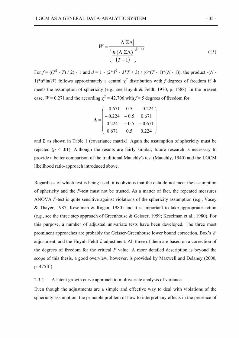
LGCM AS A GENERAL DATA-ANALYTIC SYSTEM - 35 -
(15)
For f = ((T2 - T) / 2) - 1 and d = 1 - (2*T2 - 3*T + 3) / (6*(T - 1)*(N - 1)), the product -(N -
1)*d*ln(W) follows approximately a central χ2 distribution with f degrees of freedom if Φ
meets the assumption of sphericity (e.g., see Huynh & Feldt, 1970, p. 1588). In the present
case, W = 0.271 and the according χ2 = 42.706 with f = 5 degrees of freedom for
and Σ as shown in Table 1 (covariance matrix). Again the assumption of sphericity must be
rejected (p < .01). Although the results are fairly similar, future research is necessary to
provide a better comparison of the traditional Mauchly's test (Mauchly, 1940) and the LGCM
likelihood ratio-approach introduced above.
Regardless of which test is being used, it is obvious that the data do not meet the assumption
of sphericity and the F-test must not be trusted. As a matter of fact, the repeated measures
ANOVA F-test is quite sensitive against violations of the sphericity assumption (e.g., Vasey
& Thayer, 1987; Keselman & Rogan, 1980) and it is important to take appropriate action
(e.g., see the three step approach of Greenhouse & Geisser, 1959; Keselman et al., 1980). For
this purpose, a number of adjusted univariate tests have been developed. The three most
prominent approaches are probably the Geisser-Greenhouse lower bound correction, Box’s ε̂
adjustment, and the Huynh-Feldt ε~ adjustment. All three of them are based on a correction of
the degrees of freedom for the critical F value. A more detailed description is beyond the
scope of this thesis, a good overview, however, is provided by Maxwell and Delaney (2000,
p. 475ff.).
2.3.4 A latent growth curve approach to multivariate analysis of variance
Even though the adjustments are a simple and effective way to deal with violations of the
sphericity assumption, the principle problem of how to interpret any effects in the presence of
( )
( )1
1)'(
'−
⎟⎟⎠
⎞⎜⎜⎝
⎛−ΣΛΛ
ΣΛΛ= T
Ttr
W
⎟⎟⎟⎟⎟
⎠
⎞
⎜⎜⎜⎜⎜
⎝
⎛
−−−−
−−
=
224.05.0671.0671.05.0224.0
671.05.0224.0224.05.0671.0
Λ

LGCM AS A GENERAL DATA-ANALYTIC SYSTEM - 36 -
variance and covariance changes over time remains. The multivariate approach to the analysis
of variance (MANOVA) offers a solution to this problem. As mentioned above, MANOVA
assumes several different variables (instead of a single variable whose variance is
decomposed in within- and between-subject variance), which may very well exhibit different
correlations among each other. As a matter of fact, all models introduced so far (see Figure 4
and Figure 5) are actually MANOVA models because all elements in Φ were freely estimated.
Other than the test statistics computed in repeated measures ANOVA, the multivariate
approach explicitly accounts for these variances. Returning to Equation (14), which shows the
computation of the univariate F-test, we find that by taking the trace of Φ, all off-diagonal
elements have been ignored in the ANOVA approach (i.e., all covariances were assumed to be
irrelevant). The multivariate analog of Equation (14) simply replaces the trace by the
determinant, thus taking into account all elements of Φ. Equation (16) shows the multivariate
test statistic based on the same constrained and unconstrained matrices as described above
(e.g., Maxwell & Delaney, 2000, p. 589).
(16)
In the present example (see Table 1), |ΦR| = 0.259 and |ΦF| = 0.034, so that F = 71.560
(dfnumerator = 3, dfdenominator = 32), indicating that there are indeed significant mean changes
over time (p < .01). By considering all variances and covariances among the (transformed)
measures, the F-ratio no longer depends on the assumption of sphericity14. This is a major
advantage, because the assumption of sphericity is not only very restrictive, but often
unrealistic and hardly ever met in the behavioral sciences. Other than the corrections, which
are only approximate, the multivariate approach offers an exact test of differences in means
over time. Accordingly, the type I error rates are correct even if the assumption of sphericity
is violated. On the downside, the traditional repeated measures approach has greater power to
detect any potential effects if the assumption of sphericity is met. A more comprehensive
14 While the multivariate approach does not depend on sphericity, it assumes multivariate normality which is –
strictly speaking – more restrictive than the assumption of univariate normality underlying the standard repeated
measures ANOVA. However, for practical purposes – and other than the assumption of sphericity – this
difference is typically negligible.
)1/()1/()(
+−−−
=TN
TF
F
FR
ΦΦΦ

LGCM AS A GENERAL DATA-ANALYTIC SYSTEM - 37 -
comparison of the two approaches to the analysis of change is provided by Maxwell and
Delaney (2000, chapter 13).
The LGCM likelihood-ratio test for polynomial contrasts proposed above can be easily
generalized to a test of any changes in means over time and constitutes a (new) alternative to
the multivariate F-test of Equation (16). The according test statistic corresponds to the χ2-fit
of a LGC-model as shown in Figure 5, where the means of all three growth factors (η1 - η3)
have been constrained to zero (α1 = α2 = α3 = 0). In our example χ2 = 71.483 with df = 3,
which is again highly significant (p < .01), indicating that there are significant mean changes
over time. As before, the likelihood-ratio test may be an interesting alternative in large
samples, given its ease of implementation, and its independence of the sphericity assumption.
The according Mplus syntax is identical to the syntax shown in Appendix 4, with the only
difference that the mean of the latent intercept remains unconstrained ([int*]) in both models.
While the relative advantages and disadvantages regarding type I and type II error rates of the
repeated measures ANOVA and MANOVA are comparatively well known, future research is
necessary to evaluate the performance of the likelihood-ratio test. Especially for many time
points the new approach appears to be promising, since it allows the specification of any
within-subject covariance structure. For example, it would be possible to implement the
assumption of what we might term “partial sphericity”, that is the assumption of sphericity for
a part of Φ but not the entire matrix as required by the multivariate approach. In other words,
the LGCM approach offers all advantages of MANOVA regarding potential violations of
sphericity, while being more flexible by offering the option to impose specific constraints on
the within-subject matrix. This should result in a decrease of type II errors, while type I error
rates and the correctness of parameter estimates should remain unchanged.
2.3.5 The latent growth curve modeling perspective
Putting the within-subject covariance matrix into the center of interest is probably the biggest
difference – and at the same time the greatest advancement – of LGCM over traditional
techniques. In repeated measures ANOVA the focus lies only on mean changes, while the
remaining within-subject variance is viewed as error variance and is assumed to have a very

LGCM AS A GENERAL DATA-ANALYTIC SYSTEM - 38 -
restrictive form. The MANOVA approach is more flexible with respect to the nature of the
within-subject covariance matrix (Φ), but the matrix is still treated as pure error (co)variance.
In LGCM, however, this matrix is of central interest, because it maps individual changes over
time as well as interindividual differences in individual changes. In other words, the focus is
shifted away from mean changes towards changes of individual entities (i.e., persons). To
illustrate this point, consider the model as shown in Figure 6.
Figure 6 Saturated latent growth curve model with a factor loading matrix as described in the
text.
The factor loading matrix Λ is defined as shown below and corresponds to the conventional
LGCM setup, where η0 maps true interindividual differences at the first point of measurement
(i.e., the latent intercept is positioned at the first point of measurement).
The mean of the second latent variable (η1) corresponds to the average linear increase from
one time point to the next, the mean of η2 maps the average quadratic increase and η3 the
average cubic increase. The changes in means can be described as shown in Equation (13),
with α0 = 1.112, α1 = 1.681, α2 = -0.500, and α3 = 0.111. For instance, the mean of the last
⎟⎟⎟⎟⎟
⎠
⎞
⎜⎜⎜⎜⎜
⎝
⎛
=
27931842111110001
Λ
x1 (τ1 = 0)
x2 (τ2 = 0)
x3 (τ3 = 0)
x4 (τ4 = 0)
ε1 (σ2 = 0)
ε2 (σ2 = 0)
ε3 (σ2 = 0)
ε4 (σ2 = 0)
η0 α0 = 1.112 σ2 = 0.485
η1 α1 = 1.681 σ2 = 1.721
η2 α2 = -0.500 σ2 = 1.675
η3 α3 = 0.111 σ2 = 0.098
-0.395 -1.508 -0.400
0.213 0.340
-0.037

LGCM AS A GENERAL DATA-ANALYTIC SYSTEM - 39 -
point of measurement t = 4, would be predicted to be 4τ̂ = 1.112 + 3*1.681 + 9*-0.500 +
27*0.111 = 4.66. Because the model is saturated, the predicted mean is identical to the sample
mean as shown in Table 1. In contrast to Equation (13) where any interindividual differences
are contained in the error term (εit), the interindividual differences in intraindividual change
over time are now mapped by the variance of the three growth factors. Figure 7A illustrates
this variation and Appendix 7A contains the Mplus input for the according LGC-model.
A) B)
T1 T2 T3 T40
3
6
9
T1 T2 T3 T4time
0
3
6
9
performance
T1 T2 T3 T40
3
6
9
T1 T2 T3 T40
3
6
9
T1 T2 T3 T4
0
3
6
9
T1 T2 T3 T4time
0
3
6
9
performance
T1 T2 T3 T40
3
6
9
T1 T2 T3 T40
3
6
9
Figure 7 Performance on a hypothetical learning task as introduced in Table 1. The points
along the dotted line indicate mean performance, as well as the corresponding standard
error, at each time point. The two solid lines represent the trajectories of the best and worst
individual at the last point of measurement. (A) Saturated (descriptive) model; (B) estimated
linear model.
While we see a significant increase in mean performance over time, the increase is also
characterized by large interindividual differences. As demonstrated above, this within-subject
variance is simply treated as error variance in traditional approaches. However, from Figure
7A it should also be apparent that the within-subject variance is unlikely to be unsystematic as
assumed by the repeated measures ANOVA. As a matter of fact, the fan-spread pattern of
increasing variance observed in Figure 7A is quite typical for learning data in the behavioral
sciences (Kenny, 1974; Campbell & Erlebacher, 1970). Even though the fan-spread effect
does not present a problem for the multivariate approach to the analysis of change, MANOVA
perfo
rman
ce
perfo
rman
ce

LGCM AS A GENERAL DATA-ANALYTIC SYSTEM - 40 -
still focuses on changes in means instead of providing a closer investigation of the within-
subject covariance matrix. This, however, is readily accomplished by latent growth curve
modeling. As described above, the LGC approach can be used to test the assumption of
compound symmetry or sphericity (for additional tests see Raykov, 2001), but it is also
possible to test much more refined hypotheses. For example, one might be interested in
testing the degree to which the data follow a specific trajectory over time and to what extent
individuals deviate from the average trajectory. In other words, LGCM offers great flexibility
in testing very specific hypotheses regarding change. While this can result in quite complex
models, the most basic latent growth curve models are actually very parsimonious, requiring
much fewer parameters to be estimated than standard MANOVA models. Especially applied
researchers are often not aware of this fact. Other than traditional techniques, however,
LGCM buys its advantages from the existence of a good theory. If no prior theory of mean
changes and/or individual changes can be formulated, LGCM might indeed have little value
over traditional methods. If, however, some prior theory exists, rival hypotheses can be
formulated and explicitly tested against each other. As an example, we might suspect that the
learning “curves” of the 35 individuals contained in Table 1 and depicted in Figure 7A can be
sufficiently well described by a straight line. A standard latent growth curve model as shown
in Figure 8 and as defined below, constitutes such a test. The according Mplus syntax can be
found in Appendix 7B.
Figure 8 Linear latent growth curve model.
x1 (τ1 = 0)
x2 (τ2 = 0)
x3 (τ3 = 0)
x4 (τ4 = 0)
ε1 (σ2 = .202
ε2 (σ2 = .049)
ε3 (σ2 = .325)
ε4 (σ2 = .474)
η0 α0 = 1.207 σ2 = 0.284
η1 α1 = 1.153 σ2 = 0.149
-0.031
1 1 1 1
0 1 2 3

LGCM AS A GENERAL DATA-ANALYTIC SYSTEM - 41 -
The most obvious difference to all previous models is that the variances of the error terms are
freely estimated and are no longer constrained to zero. By imposing a theory of change on the
data, the within-subject variance-covariance matrix Φ could be further partitioned into mean
changes over time, systematic individual deviations from the average (linear) trajectory, and
time point specific residual variances represented by Θε. It is important to note that the
partitioning of the within-subject variance into “systematic” variance contained in Φ and
“error” variance (Θε) is contingent on the underlying theory of change. In that sense it is
difficult to distinguish between systematic time point specific variance and pure measurement
error, or more generally to distinguish between reliability and validity of change (Voelkle,
2005). Figure 7B shows the estimated individual trajectories using a linear LGC-model. If the
usual assumptions of structural equation models are met (primarily multivariate normality)
and sample size is large enough, the resulting model fit provides a test of the goodness of
approximation of the estimated trajectories to the observed trajectories shown in Figure 7A.
The evaluation and interpretation of fit indices works as usual and will not be reviewed in this
thesis (but see Bollen & Long, 1993; Schermelleh-Engel, Moosbrugger, & Müller, 2003).
Note, however, that it is also possible to compare competing models of change (nested and
non-nested, see Levy & Hancock, 2007). For example, by adding a quadratic growth
component, it could be easily tested whether a quadratic growth curve model fits the data
significantly better than a linear one. In the present example, the linear model as shown in
Figure 8 results in χ2 = 6.180 with 5 degrees of freedom (p > .05), indicating a good model fit.
After introducing an additional quadratic growth factor as shown in Figure 9, the fit improves
slightly (χ2quadratic =4.138) but the improvement is not significant (χ2
Diff = χ2linear - χ2
quadratic =
6.180 - 4.138 = 2.042 with dflinear - dfquadratic = 5 - 1 = 4, p > .05) so that the more
parsimonious linear model would be retained. The Mplus input for the quadratic LGC-model
is provided in Appendix 7C.
⎟⎟⎟⎟⎟
⎠
⎞
⎜⎜⎜⎜⎜
⎝
⎛
=
4
3
2
1
xxxx
x ⎟⎟⎠
⎞⎜⎜⎝
⎛=
1
0
ηη
η
⎟⎟⎟⎟⎟
⎠
⎞
⎜⎜⎜⎜⎜
⎝
⎛
=
31211101
Λ
⎟⎟⎟⎟⎟
⎠
⎞
⎜⎜⎜⎜⎜
⎝
⎛
=
0000
τ ⎟⎟⎠
⎞⎜⎜⎝
⎛= 2
10
2
1
0
η
η
σφσ
Φ⎟⎟⎠
⎞⎜⎜⎝
⎛=
1
0
αα
Α
⎟⎟⎟⎟⎟
⎠
⎞
⎜⎜⎜⎜⎜
⎝
⎛
=
4
3
2
1
εεεε
ε ⎟⎟⎠
⎞⎜⎜⎝
⎛= 2
2
2
1
0 ε
ε
σσ
εΘ

LGCM AS A GENERAL DATA-ANALYTIC SYSTEM - 42 -
Figure 9 Quadratic latent growth curve model.
In the linear model, the means of the latent intercept and the latent slope are both significant
(α0 = 1.207, p < .01, α1 = 1.153, p < .01) indicating that average performance in the learning
task is significantly different from zero at the first point of measurement and that people
exhibit a significant mean improvement of about 1.153 units from one time point to the next.
In this regard, LGCM is similar to repeated measures ANOVA, in that it shows that the means
differ over time. By imposing a linear trajectory, however, we also test the shape of the
overall curve, which can be well described by a straight line as suggested by the good model
fit. In addition to mean changes, there are significant interindividual differences in true initial
performance indicated by the significant variance of the latent intercept (σ2(η0 ) = 0.284, p <
.01). Finally, people show significant interindividual differences in their improvement over
time. This was already suggested by the strong fan-spread pattern in Figure 7A and is mapped
by the significant variance of the linear latent growth curve factor (σ2(η1) = 0.149, p < .01).
As illustrated by Figure 7A and B, the mean changes, as well as the interindividual
differences in initial performance and change over time, are well described by a linear latent
growth curve model. As an alternative, it is also possible to permit (some of) the factor
loadings to be freely estimated. This gets close to traditional confirmatory factor analysis
(CFA), where no predefined growth curves are imposed on the data. In the present example
we could modify the linear LGCM by allowing the last two factor loadings of η1 to be freely
estimated and let the data “tell us” the best shape of the trajectory. This would fit a “linear
spline” to the data (see Meredith & Tisak, 1990), resulting in the two loadings λ31 = 1.772 and
0.049
x1 (τ1 = 0)
x2 (τ2 = 0)
x3 (τ3 = 0)
x4 (τ4 = 0)
ε1 (σ2 = .251
ε2 (σ2 = .002)
ε3 (σ2 = .385)
ε4 (σ2 = .248)
η0 α0 = 1.154 σ2 = 0.236
1 1 1 1 0
1 2 3
η2 α2 = -0.047 σ2 = 0.011
-0.007
-0.019
0 1 4 9
η1 α1 = 1.297 σ2 = 0.109

LGCM AS A GENERAL DATA-ANALYTIC SYSTEM - 43 -
λ41 = 2.767 and a model fit of χ2 = 1.558 with 3 degrees of freedom. However, because the
improvement in model fit over the more restrictive linear model is not significant (χ2Diff =
6.180 - 1.558 = 4.622 dfDiff = 2, p > .05), the more parsimonious linear LGCM should be
retained. Regardless of whether the factor loadings are freely estimated or fixed based on an
existing theory, the present example illustrated that LGCM combines the analysis of mean
changes, as provided by traditional analysis of variance techniques, with a more detailed
analysis of the within-subject covariance matrix. It is this shift in focus – away from group
changes towards individual changes – which makes LGCM such a versatile and promising
technique.
To summarize, it has been shown that repeated measures ANOVA and MANOVA are
essentially special cases of the more general latent growth curve modeling approach. That
being said, differences exist with respect to the underlying estimation procedure. LGC-models
are typically based on (large-sample) ML estimation, while least square estimation is
employed for (finite-sample) ANOVA and MANOVA type models. Different estimation
techniques are based on different assumptions (e.g., multivariate normality and/or a
sufficiently large sample) and will produce different results based on the degree to which the
assumptions are met in a given sample. A more detailed comparison of different estimation
techniques is beyond the scope of this section (but see Bollen, 1989), and I settle for a
comparison on the model level in the present thesis. Regarding model specification, however,
it has been shown that the standard repeated measures ANOVA is identical to a LGC-model
with the assumption of a spherical covariance matrix among the latent growth factors. Based
on research by Raykov (2001) it was demonstrated that the assumption of compound
symmetry and sphericity can be easily tested within the LGCM framework and a likelihood-
ratio based alternative to Mauchly’s criterion W has been proposed. Likewise, alternative
likelihood-ratio tests were proposed for polynomial contrasts, which have been demonstrated
to be easily incorporated into the general latent growth curve approach. Other than repeated
measures ANOVA, neither the multivariate analysis of variance, nor LGCM rests on the
assumption of sphericity. As a matter of fact, the saturated LGC-model is equivalent to
MANOVA, but other than MANOVA, latent growth curve modeling allows the researcher to
impose specific constraints on the covariance matrix of the latent variables. Again, a

LGCM AS A GENERAL DATA-ANALYTIC SYSTEM - 44 -
likelihood-ratio test has been proposed as an alternative to the multivariate F-test employed in
MANOVA, but future research is necessary to evaluate the validity of such a test. Finally, it
has been argued that LGCM is characterized by a shift in focus, away from the analysis of
mean changes, towards the analysis of individual trajectories. This change in perspective is
characterized by (a) the possibility to formulate and test much more sophisticated hypotheses
regarding the within-subject covariance matrix than possible with traditional methods. The
need to have a good theory underlying one’s model specification (b), and great flexibility of
incorporating predictors of change (c), which will be the topic of the next section.
2.4 Predicting change
The biggest advantage of being able to better describe (individual) changes over time is the
possibility to better predict these changes. In this section it will be demonstrated how to use
categorical and continuous variables to explain interindividual differences in change.
Traditional methods will be compared to the more general LGCM approach. As before, I will
proceed in three steps by first considering two-wave data before moving to more complex
multi-wave designs. Finally, some more recent developments will be outlined.
2.4.1 Predicting change in two-wave data
The prediction of pre- to post-test change is very straightforward. As demonstrated in the first
section, a paired samples t-test corresponds to a latent growth curve model as shown in Figure
2A. This model can be easily extended by regressing η0 and/or η1 on potential predictors as
illustrated by Figure 10A. As also discussed above, the paired samples t-test is identical to an
independent t-test on the difference scores (i.e., x4 - x1). Thus, a regression of η1 on group
membership is identical to the regression of the difference scores on group membership, as
long as the error variances of x4 and x1 are constrained to zero. Likewise, a regression of the
observed difference scores on one or more categorical and/or continuous variables is identical
to the prediction of η1 by the same predictors.

LGCM AS A GENERAL DATA-ANALYTIC SYSTEM - 45 -
A) B)
Figure 10 Path diagram of a paired samples t-test (A) and a base-free measure of change
model (B) using either “sex” or “g” as predictor for individual difference in pre- to posttest
(x1 to x4) changes (sex // g). The predictor g is z-standardized. Men are coded as 1 and women
as 0.
Figure 10A illustrates this fact for either sex or g as predictor of initial performance (η0) and
change over time (η1). Appendix 8 contains the according Mplus syntax. If the independent
variable is in deviation form (i.e., its mean is zero), the intercept of the dependent variable
corresponds to its mean (e.g., Aiken & West, 1991). For this purpose, g was z-standardized
prior to including it as a predictor. Now, the mean of the latent growth factor (α1 = 3.549) is
equal to the mean difference between pre- and post-test. As demonstrated in the first section
(see Equation (5)), this difference is highly significant (p < .01). By regressing η1 on g, a
regression coefficient (γ1g = 0.539) is obtained, which maps the difference in improvement
from pre- to post-test between people with an average intelligence (i.e., g(standardized) = 0)
and people one standard deviation above average (g(standardized) = 1). Dividing the
coefficient by its standard error (S.E. = 0.223), we find that the difference in mean
performance is significant (p < .05). The same is true for the prediction of η0, where the
regression coefficient (γ0g = -0.031) indicates that people one standard deviation above
average on g, start off somewhat worse at the beginning of the learning task as compared to
1 1 1 0
x1
x4
ε1 ε4
η0 α0 = 0.817 //
1.112
η1 α1 = 2.984 //
3.549
sex // g
1.099// 0.539
0.573//-0.031
ζ1
-0.427 // -0.254
1.666 // 1.685ζ0
0.403 // 0.485
1 1 1 0
x1
x4
ε1 ε4
η0 α0 = 0.817 //
1.112
η1 α1 = 3.863 //
3.992
sex // g
1.716// 0.527
0.573//-0.031
ζ1
0.919 // 1.228ζ0
0.304 // 0.385
-1.077 // -0.399

LGCM AS A GENERAL DATA-ANALYTIC SYSTEM - 46 -
people with an average intelligence. The difference, however, is small and not significant
(S.E. = 0.119, p > .05). The same interpretation holds for using the categorical variable gender
instead of g as a predictor (see again Figure 10A). In the example women are coded as zero,
so the mean of η0 corresponds to the average performance of women at the first point of
measurement. The regression coefficient (γ0sex = 0.573) indicates that men are slightly better
than women in their initial performance and dividing γ0sex by its standard error reveals that
this difference is indeed significant (S.E. = 0.215, p < .05). Likewise, men show a larger
improvement from pre- to post-test than women. On average, women improve about α1 =
2.984 units as compared to an increase of α1 + γ1sex = 2.984 + 1.099 = 4.083 units of men. The
difference is again significant (γ1sex = 1.099, S.E. = 0.437, p < .05). The test is asymptotically
equivalent to the independent samples t-test (using the pre-post difference scores (x4 - x1) as
dependent variable) and the repeated measures ANOVA for two time points and one
(categorical) between-subject factor. Table 3 compares the LGCM estimate (γ1sex) with the
results of a t-test and repeated measures ANOVA obtained by using any major statistical
software package.
Table 3 Independent samples t-test, repeated measures ANOVA and LGCM approach to
testing the difference in pre- to post-test improvement between men and women. Note that
(asymptotically) all three approaches will yield identical results.
Independent samples t-test Mean difference (x4 - x1) t df p
1.099 -2.444 33 .020 Repeated measures ANOVA
F df p Source Time 246.979 1 .000 Time*sex 5.972 1 .020
LGCM Estimate (γ1sex) Standard error (SE) p 1.099 0.437 .020
Note: t2 = F for dfnumerator = 1.
Finally, the covariance between ζ0 and ζ1 maps the relationship between pre- and post-test
after controlling for any predictors. Using gender as a predictor, there is a slight, but

LGCM AS A GENERAL DATA-ANALYTIC SYSTEM - 47 -
significant correlation between pre- and posttest (φ01 = -0.427, corr = -0.437, S.E. = 0.156, p
< .05), while the correlation gets smaller and is no longer significant after controlling for g
instead of gender (φ01 = -0.254, corr = -0.259, S.E. = 0.159, p > .05). This suggests that part
of the covariation between pre- and post-test is “caused” by intelligence. However, because
the sample size is small (and of course the fact that the data were chosen for illustrative rather
than substantive purposes) one must be careful in interpreting this finding.
As demonstrated in Section 2.2.2, the LGCM approach allows us to take the reliabilities of x1
and x4 into account, should they be known. Likewise, predictors can be included in the base-
free measure of change model as shown in Figure 10B. Appendix 9 contains the according
Mplus input for the base-free measure of change model and reliability corrected indicators.
Now, the effect of gender on improvement (η1) is independent of any prior performance. That
is, if men and women had started out equal on the learning task, they would still differ in their
change from pre- to post-test by about 1.716 units. This difference is larger than in the
previous (difference score) model and is highly significant (γ1sex = 1.716, S.E. = 0.435, p <
.05). The effect of gender on η0 remains unaffected by analyzing residualized (true) gain
scores instead of direct difference scores. However, it is now possible to obtain and test the
indirect effect of gender via η0 on η1. The estimate is simply computed by multiplying β10
with γ0sex. The standard error is readily provided by Mplus (command IND in Appendix 9).
The indirect effect (γ0sex*β10 = 0.573*-1.077= -0.617), however, is not significant (S.E. =
0.322, p > .05). The same procedure can be adopted in testing the direct and indirect effects
of g instead of sex (see Figure 10B and Appendix 9). Note, that the LGCM approach makes
no difference between categorical and continuous predictors. This stands in contrast to the
repeated measures ANOVA, where the between-subject factor must be categorical. If this is
the case, the results are identical as shown in Table 3. ANOVA, however, cannot be employed
if g would be used as a predictor instead of gender. In the case of two-wave data, taking the
difference between x4 and x1 and regressing it on any continuous predictor easily circumvents
this problem. This cannot be done in multi-wave data as will be discussed in the next section.
In addition, the predictor is assumed to be measured without error in standard regression or
ANOVA type procedures. This is also no longer true for the LGCM approach, where we can
easily adjust for unreliability of the predictor in the same way the dependent variable(s) were

LGCM AS A GENERAL DATA-ANALYTIC SYSTEM - 48 -
adjusted for unreliability. Moreover, the independent variables need not be directly observed,
but may be latent. This is only possible using the LGCM approach.
Of course more than one predictor can be considered at a time and it is possible to include
interactions among predictors. All this is not different from any standard regression analysis
and shall not be reviewed in this section (but see Cohen et al., 2003; Aiken & West, 1991). In
structural equation modeling, multiple group analysis is another option to test hypotheses
involving categorical (grouping) variables. An introduction to multiple group analysis can be
found in any SEM textbook (e.g., Bollen, 1989, p. 355ff.). One advantage of multiple group
analysis is the possibility to test for differences in variances across groups instead of being
limited to mean differences as it is the case in linear regression. From the previous analyses
we know that men are significantly better in true initial performance, as well as improvement
from pre- to post-test. Accordingly, we might set up a model, which accounts for this fact by
allowing the means of the two latent variables to differ across groups. In a next step, however,
it might be interesting to see whether men are not only better, but exhibit larger
interindividual differences as compared to women. This test is readily implemented by
comparing a model where the variances of η0 and η1 are constrained to equality across groups
to a model where the variances are allowed to be freely estimated. Figure 11 shows the
parameter estimates of the unconstrained model and Appendix 10 contains the according
Mplus syntax.
Men: Women:
Figure 11 Multiple group analysis using gender as grouping variable. All freely estimated
parameters are allowed to differ across groups (saturated model).
1 1 1 0
x1
x4
ε1 ε4
η0 α0 = 1.390 σ2 = 0.627
η1 α1 = 4.082 σ2 = 1.646
-0.650
1 1 1 0
x1
x4
ε1 ε4
η0 α0 = 0.817 σ2 = 0.167
η1 α1 = 2.984 σ2 = 1.687
-0.190

LGCM AS A GENERAL DATA-ANALYTIC SYSTEM - 49 -
Constraining both variances to equality (σ2(η0men) = σ2(η0women) = 0.408, S.E. = 0.097, p < .01
and σ2(η1men) = σ2(η1women) = 1.602, S.E. = 0.382, p < .01), we obtain a model fit of χ2 = 7.546
with 2 degrees of freedom. Allowing the variances to differ, the model is just identified with
zero degrees of freedom, so the χ2 reported above indicates that the two variances (taken
together) differ significantly across groups (p < .05). As apparent from Figure 11, men exhibit
an over three times larger variance at the pre-test, while the post-test variance is almost
identical for men and women (σ2(η0men) = 0.627, S.E. = 0.209, p < .05; σ2(η1men) = 1.646, S.E.
= 0.549, p < .05 and σ2(η0women) = 0.167, S.E. = 0.057, p < .05; σ2(η1women) = 1.687, S.E. =
0.579, p < .05). As a matter of fact, when constraining the post-test variance to equality, the
drop in fit is negligible suggesting that men and women do not differ in their variability of
pre- to post-test change (χ2Diff = 7.546 - 7.056 = 0.49, dfDiff = 2 - 1 = 1, p > .05). Reintroducing
g as a predictor of η0 and η1 allows us to test (possibly quite sophisticated) interaction
hypotheses. For example, by comparing a model where γ1g is constrained to equality across
the two groups to a model where γ1g is allowed to differ is equivalent to testing an interaction
between g and sex. A significant χ2Diff would suggest that the effect of g on pre- to post-test
change differs between men and women. One can think of numerous other hypotheses, which
are readily formulated and tested within this general framework. As discussed in Section
2.2.2, the LGCM approach gets particularly interesting if more than one (parallel) measure
was obtained at each time point, so that the error terms can be estimated rather than being
constrained a priori (see Figure 3).
2.4.2 Predicting change in multi-wave data
The option to use difference scores as dependent variable in a pre- to post-test analysis makes
it easy to analyze and predict change in two-wave data. This is no longer true for the
prediction of change over multiple waves. As discussed in the previous section, traditional
methods are often based on very restrictive assumptions, such as compound symmetry or
sphericity, which still apply when it comes to the prediction of change. Furthermore, there are
additional assumptions that must be met when including predictors. Finally, the exclusive
focus on mean changes – instead of individual trajectories – restricts MANOVA and ANOVA
to the use of categorical predictors. The more general LGCM approach is not only more
flexible with respect to those assumptions, but offers a convenient way to test them.

LGCM AS A GENERAL DATA-ANALYTIC SYSTEM - 50 -
Moreover, it is not limited to categorical predictors but allows for any combination of
categorical and/or continuous variables.
Using the same factor loading matrix as before,
η0 is again “centered”, mapping average interindividual differences across all four time points.
Thus, a regression of η0 on a categorical predictor corresponds to the between-subject analysis
in a repeated measures ANOVA. Figure 12 shows the according path diagram for our
example data set. Appendix 11 contains the Mplus input.
Figure 12 Repeated measures (M)ANOVA with one between (sex) and one within (time)
subject factor, where only between-subject variance is predicted by sex (no interaction
between time and sex). Parameter estimates on the right side of the graph are obtained when
fixing the regression coefficient of η0 on sex to zero (γ0sex = 0).
⎟⎟⎟⎟⎟
⎠
⎞
⎜⎜⎜⎜⎜
⎝
⎛
−−−−
−−
=
224.05.0671.05.0671.05.0224.05.0
671.05.0224.05.0224.05.0671.05.0
Λ
x1 (τ1 = 0)
x2 (τ2 = 0)
x3 (τ3 = 0)
x4 (τ4 = 0)
ε1 (σ2 = 0)
ε2 (σ2 = 0)
ε3 (σ2 = 0)
ε4 (σ2 = 0)
η0 α0 = 4.624
η1 α1 = 2.594 σ2 = 1.063
η2 α2 = 0.001 σ2 = 0.255
η3 α3 = 0.150 σ2 = 0.177
0.114
0.061 0.015
sex
ζ0 σ2 = 1.197
0.066
-0.013
0.509 1
2.230
0.220
0.004
-0.045
αsex = 0.514
σ2sex = 0.250
α0 = 5.771
α1 = 2.594
α2 = 0.001
α3 = 0.150
σ2(ζ0) = 2.439
σ2(η1) = 1.095
φ01 = 1.036
φ02 = 0.124
φ03 = -0.027
φ12 = 0.092
φ13 = 0.052
φ23 = 0.118
φsex1 = -0.017

LGCM AS A GENERAL DATA-ANALYTIC SYSTEM - 51 -
Constraining the regression coefficient γ0sex to zero, the variance of η0 (σ2(η0) = σ2(ζ0) =
2.439) corresponds to the between-subjects sum of squares divided by N (35*2.439 = 85.36 =
SSBetween; see Table 2). When regressing η0 on gender (γ0sex = 2.230), the remaining variance
corresponds to the variance not accounted for by sex (σ2(ζ0) = 1.197), so that the sum of
squares explained by sex are SSBetween(sex) = 85.36 - 35*1.197 = 43.47, corresponding exactly
to the SSBetween(sex) obtained by any standard software package. Likewise, F =
(SSBetween(sex)/dfBetween) / (SSBetween(error)/dfBetween(error)) = (43.47/1) / (41.89/33) = 34.25,
suggesting that there are significant differences in mean performance between men and
women (p < .01). Since the variance of the other factors is not affected by the introduction of
a predictor, the change over time can be evaluated as discussed above (compare Figure 12 and
Figure 5). However, while the prediction of interindividual differences in average
performance does not depend on the within-subject covariance matrix (Φ), the analysis of
interindividual differences in change over time does. In addition, the introduction of a
categorical predictor requires that the variance-covariance matrix (Φ) is identical across all
levels of the predictor (in our example for men and women). It is important to note that the
two assumptions of sphericity and homogeneity of variance are independent, so it can easily
happen that one assumption is met, while the other is not (Maxwell & Delaney, 2000, p. 534).
This makes the estimation of an interaction between a within-subject factor and a between-
subject factor much more demanding. The prediction of within-subject variance is easily
implemented by regressing all growth factors (η1 – η3) on the independent variable(s) in
question. Figure 13 shows the according path diagram (with Λ as shown above) and Appendix
12 contains the Mplus syntax. As a reminder, the within-subject main effect due to time can
be computed by constraining the means of η1 – η3 to zero (in addition to setting γ1sex = γ2sex =
γ3sex = 0), and comparing the sum of the residual variances to the sum of residual variances
after allowing the means to be freely estimated.

LGCM AS A GENERAL DATA-ANALYTIC SYSTEM - 52 -
Figure 13 Repeated measures (M)ANOVA with one between (sex) and one within (time)
subject factor. Interindividual differences in change over time are predicted by sex
(interaction between time and sex). Parameter estimates on the right side of the graph are
obtained when setting the regression coefficients γ1sex = γ2sex = γ3sex = 0.
The prediction of change by gender corresponds to an interaction effect of the between-
subject factor sex and the within-subject factor time. This is readily apparent from Figure 13
where the effect of sex on x is mediated by η. This is not true for the prediction of the
between-subject variance, because all factor loadings of η0 are identical, thus the effect is
simply multiplied by a constant. For example – and as shown above – if all factor loadings of
η0 are constrained to 0.5, the variance of η0 corresponds to the average between-subject
variance, while the mean (α0 = 4.624) must be divided by two in order to obtain the average
performance of women on the learning task ( womenx = 2.312). When setting γ1sex = γ2sex = γ3sex
= 0, the sum of the variances of η1 to η3 is 1.063 + 0.255 + 0.177 = 1.495. Multiplying 1.495
by the number of subjects, the sum of squares between persons is SSBetween = 35*1.495 =
52.325, which is the sum of squares after controlling for the within-subject factor time (note
that α1 to α3 are freely estimated). The resulting sum of squares can be further partitioned into
one part which is due to gender differences and one part which is independent of gender and
x1 (τ1 = 0)
x2 (τ2 = 0)
x3 (τ3 = 0)
x4 (τ4 = 0)
ε1 (σ2 = 0)
ε2 (σ2 = 0)
ε3 (σ2 = 0)
ε4 (σ2 = 0)
η0 α0 = 4.624
η1 α1 = 2.142
η2 α2 = -0.006
η3 α3 = 0.243
sex
ζ0 σ2 = 1.197
0.0152.230
0.061
αsex = 0.514
σ2sex = 0.250
ζ1 σ2 = 0.870
ζ2 σ2 = 0.255
ζ3 σ2 = 0.169
0.055
0.509 0.063 0.115
-0.013
-0.1810.879α0 = 4.939
α1 = 2.594
α2 = 0.001
α3 = 0.150
σ2(ζ0) = 1.290
σ2(ζ1) = 1.063
σ2(ζ2) = 0.255
σ2(ζ3) = 0.177
φ01 = 0.643
φ02 = 0.063
φ03 = -0.041
φ12 = 0.066
φ13 = 0.015
φ23 = 0.114
γ0sex = 1.617
γ1sex = 0
γ2sex = 0
γ3sex = 0

LGCM AS A GENERAL DATA-ANALYTIC SYSTEM - 53 -
independent of mean changes over time. This is readily computed by reintroducing the direct
effects of sex on η1, η2 and η3. The estimates are shown in Figure 13. The sum of the
variances of η1 to η3 is 0.870 + 0.255 + 0.169 = 1.294. After multiplication with N, this
corresponds to the SSWithin(error) after accounting for changes over time (main effect time)
and gender differences in change over time (time*sex), and is identical to the SSWithin(error)
obtained by any conventional software package (SSWithin(error) = 45.29). As a consequence,
the interaction between time and sex can be easily computed by subtracting 45.29 from
52.325, resulting in an effect of SSWithin(time*sex) = 7.035. The F-test can be computed
accordingly, with F = (SSWithin(time*sex)/dfWithin(time*sex)) / (SSWithin(error)/dfWithin(error)) =
(7.035/3) / (45.29/((35-2)*(4-1))) = 5.13 suggesting that men and women differ significantly
in their change over time (p < .05).
In order for the F-value to be a reasonable test statistic, not only the assumption of sphericity
must be met, but also the assumption of equal variances and covariances across groups (i.e.,
the homogeneity of variance assumption). The latter is true for the traditional repeated
measures approach as well as the LGCM approach. If the assumption is not met, it would not
make sense to compare mean changes across groups, since the within-subject error terms (i.e.,
the residual within-subject (co)variance matrix) would differ, making it a futile comparison.
Other than ANOVA or MANOVA, however, LGCM provides not only a direct test of this
assumption, but offers an alternative to the F-ratio, which neither depends on the assumption
of sphericity nor on the assumption of variance homogeneity. For this purpose, gender is not
treated as an exogenous variable, but as a grouping variable in a multiple-group analysis, as
described above. Figure 14 shows the according model and Appendix 13 the Mplus input.

LGCM AS A GENERAL DATA-ANALYTIC SYSTEM - 54 -
Men: Women:
Figure 14 Multiple group analysis using gender as grouping variable. All freely estimated
parameters shown in the path diagram are allowed to differ between groups (saturated
model). Parameter estimates on the left side of the graph are obtained when all variances and
covariances of the four factors are constrained to equality, but the means are allowed to
differ across groups. Comparing the two models tests the assumption of variance
homogeneity.
The assumption of variance homogeneity can be simply tested by comparing a model where
all elements in Φ are constrained to equality across groups15 to a model where all elements in
Φ are allowed to differ (see Raykov, 2001). Since the two models are nested, a likelihood-
ratio test can be carried out to test the significance of any differences between the models.
15 Constraining all elements (i.e., means, variances and covariances) to equality across groups results in the same
parameter estimates as shown in Figure 5. However, because the factor loadings of η0 are now constrained to 0.5
(instead of 1.0 as in Figure 5), all estimates associated with η0 in Figure 5 must be multiplied by two in order to
obtain the same estimates.
x1 (τ1 = 0)
x2 (τ2 = 0)
x3 (τ3 = 0)
x4 (τ4 = 0)
ε1 (σ2 = 0)
ε2 (σ2 = 0)
ε3 (σ2 = 0)
ε4 (σ2 = 0)
η0 α0 = 4.624 σ2 = 1.028
η1 α1 = 2.142 σ2 = 0.824
η2 α2 = -0.006 σ2 = 0.205
η3 α3 = 0.243 σ2 = 0.225
0.652 0.224 0.147
0.181 0.132
0.145
x1 (τ1 = 0)
x2 (τ2 = 0)
x3 (τ3 = 0)
x4 (τ4 = 0)
ε1 (σ2 = 0)
ε2 (σ2 = 0)
ε3 (σ2 = 0)
ε4 (σ2 = 0)
η0 α0 = 6.854 σ2 = 1.356
η1 α1 = 3.021 σ2 = 0.913
η2 α2 = 0.008 σ2 = 0.301
η3 α3 = 0.062 σ2 = 0.116
0.373 -0.089 0.084
-0.053 -0.017
-0.163
σ2(η0) = 1.197
σ2(η1) = 0.870
σ2(η2) = 0.255
σ2(η3) = 0.169
φ01 = 0.509
φ02 = 0.061
φ03 = -0.013
φ12 = 0.063
φ13 = 0.055
φ23 = 0.115

LGCM AS A GENERAL DATA-ANALYTIC SYSTEM - 55 -
Technically speaking, the null-hypothesis (H0) states that Φ(men) = Φ(women), while the
alternative hypothesis assumes that there are significant differences between the covariance
matrices of the two groups (H1: Φ (men) ≠ Φ(women)). For T repeated measures, the within-
subject matrix contains T*(T + 1)/2 non-redundant elements, resulting in a χ2-difference test
with 4*5/2 = 10 degrees of freedom in the present example. The test of variance homogeneity
is readily implemented by constraining all ten elements in Φ to equality across groups as
shown in Appendix 13. The means of the latent variables are allowed to differ across groups
and may be freely estimated. The constrained model results in a χ2 of 18.262 with 10 degrees
of freedom. Since this value must be compared to a saturated model with χ2 = 0, the model fit
indicates that the homogeneity assumption may be met (p > .05). As before, the reader is
reminded that the test is actually a large sample test and its performance is not very well
known in small samples. In large samples, however, it might be an interesting alternative to
the popular Box M test (Box, 1949) as pointed out by Raykov (2001).
(17)
As shown in Equation (17), Box’s M statistic is also based on the likelihood-ratio test. G is
the number of groups (g = 1…G; e.g., males and females), Ng is the sample size in each
group, and Sg the within group covariance matrix. S is the covariance matrix pooled across all
groups (i.e., )/()1(1
gNN gG
g g −−= ∑ =SS ). In the present example, M = 17.183. For small
samples an F approximation is used to compute its significance, indicating that the covariance
matrices are not significantly different across groups (F = 1.491, df1 = 10, df2 = 5163.441, p >
.05; see Box (1949) for details). This stands in contrast to the assumption of sphericity, which
was clearly violated. Notice that sphericity was not tested by either of the two tests, although
a combined test of sphericity and variance homogeneity would be possible using the LGCM
approach. With respect to variance homogeneity, the LGCM based test and Box’s test yield
very similar results in our example. However, since the LGCM approach requires large
samples, Box’s M statistic may be better suited for small sample sizes. Having said that,
Box’s test appears to be overly sensitive to non-normality (Tabachnick & Fidell, 2001;
Stevens, 2002), a problem that might be less severe for the LGCM based test with large
gSS log)1(log)(1
−−−= ∑=
G
ggNGNM

LGCM AS A GENERAL DATA-ANALYTIC SYSTEM - 56 -
sample sizes. Future research might address this apparent trade-off by means of a Monte
Carlo Simulation.
The LGCM approach offers not only a direct test of the assumptions of sphericity and/or
homogeneity of variance, but can account for these violations. The multiple group analysis
allows researchers to formulate and implement very specific hypothesis regarding possible
group differences in Φ. Given the usual assumptions of structural equation models are met
(primarily multivariate normality and/or a sufficiently large sample size), the resulting
parameter estimates and significance tests (i.e., likelihood-ratio tests) are correct. Note that
this is not true for the F-ratio as described above, which always depends on the assumption of
variance homogeneity across groups. Another important advantage of LGCM is the option to
use continuous predictors instead of categorical predictors. This is not possible in standard
ANOVA or MANOVA and opens up a wide field of new applications. In the example this
would simply mean replacing sex by g in Figure 12 and Figure 13 as well as Appendix 11 and
Appendix 12. Finally, it is straightforward to combine the use of continuous and/or
categorical exogenous predictors and multiple group analysis (i.e., categorical predictor). This
is a great improvement over traditional techniques, because it allows a detailed analysis of
interindividual differences in individual change over time making use of all available
information (e.g., no need for categorization of continuous predictors). At the same time, the
assumptions of variance homogeneity and sphericity are no longer indispensable, but may be
relaxed if necessary. However, future research is necessary to explore the differences of the
approaches with respect to accuracy, power and robustness under various conditions. The
great flexibility of LGCM is certainly an advantage, but also calls for a thorough matching of
theory and statistical modeling. Eventually, it is up to the researcher to define the most
appropriate model for his or her purposes.
2.4.3 Extensions
As mentioned in the introduction (Section 1.1.2), the basic latent growth curve model has
been extended in numerous ways during the last couple of years. An overview of these
extensions is provided for example by Bollen and Curran (2006), Duncan, Duncan and
Strycker (2006), or in the excellent book edited by Moskowitz and Hershberger (2002). With

LGCM AS A GENERAL DATA-ANALYTIC SYSTEM - 57 -
respect to the prediction of change, however, there are at least three extensions worth
mentioning. First, the effect of any time-invariant predictor on x must not necessarily be
mediated by the growth factors but may be direct and time-varying (Stoel, van den
Wittenboer, & Hox, 2004; Muthén, 1991). This is easily accomplished by regressing x
directly on the predictor(s) with all regression weights allowed to be freely estimated. Second,
the predictors themselves can change over time, what is not possible in traditional repeated
measures ANOVA or MANOVA designs (e.g., Bollen & Curran, 2006, p. 192ff.). The impact
of time-varying predictors may again change over time or be time-invariant (i.e., the
regression weights are constrained to equality). Third, it is possible to estimate parallel
growth processes with average performance and/or rate of change of one process affecting
average performance and/or rate of change on another variable. An introduction is given for
example by Bollen and Curran (2006, p. 198ff.), or Curran and Willoughby (2003). Finally,
the LGCM approach has been combined with other techniques to analyze change over time
such as the autoregressive model (Bollen & Curran, 2004), which will be discussed in more
detail in Section 3. All of these extensions are not possible with traditional techniques like the
paired samples t-test, ANOVA or MANOVA, making a comparison impossible. For more
detailed information on these extensions, the interested reader is referred to the above-
mentioned literature.
To summarize, it has been shown that LGCM is a very general approach to the prediction of
change. The conventional t-test, repeated measures ANOVA and MANOVA are all special
cases of the more general latent growth curve approach. For the simplest case of only two
time points, the use of difference scores constitutes an easy way to analyze interindividual
differences in change. In this case, and for only two groups, the independent samples t-test,
repeated measures ANOVA with one between-subject factor, MANOVA and LGCM as
shown in Figure 10A yield identical results. In addition, the LGCM approach offers a
convenient way to analyze and predict residualized (true) gain scores. Finally, LGCM can
account for imperfect reliability of the criterion and/or predictor. Especially for more complex
models with multiple measurements taken at each time point and complex (latent) predictors
this is a great improvement over traditional techniques. For multi-wave data it has been
shown that the repeated measures design with one between- and one within-subject factor
(also known as split-plot or mixed design, see Maxwell & Delaney, 2000, p. 517ff.) can be

LGCM AS A GENERAL DATA-ANALYTIC SYSTEM - 58 -
easily incorporated into the more general LGCM approach. Other than the traditional
methods, however, LGCM is not limited to the use of categorical predictors. As a matter of
fact, quite complex interaction hypotheses including categorical and/or continuous predictors
can be tested. The assumption of variance homogeneity across groups, which is crucial for
repeated measures ANOVA and MANOVA, can be tested within the LGCM framework, but
other than ANOVA or MANOVA, LGCM can also account for violations of this assumption
by offering an alternative to the conventional F-test. The most striking difference between
LGCM and ANOVA/MANOVA is the greater flexibility of the former as compared to the
latter. While this is certainly an advantage, it demands great diligence from the researcher
when setting up the model and interpreting results.
2.5 Discussion
By demonstrating that the analysis of variance and multiple regression are essentially
identical data analytic systems, Cohen (1968) prepared the ground for a new way of statistical
thinking among social scientists. Instead of treating ANOVA and multiple regression as
different techniques, he pointed to the generality of MR, which comprises the analysis of
variance as a special case. This prepared the ground for more refined analyses regarding
group differences and interindividual differences, helping ultimately to bridge the gap
between experimental and differential psychology. In this section it has been argued that it is
time for a similar reconceptualization in the analysis of change. During the last decade there
has been an almost exponential increase in methodological and applied articles using “new
methods for the analysis of change” (Collins & Sayer, 2001). The new procedures focus on
intraindividual variability instead of mean changes, which have been of central interest in
traditional methods such as the paired samples t-test, repeated measures ANOVA or
MANOVA. The notion that the latter are just a special case of the former has always been
present (Meredith & Tisak, 1990), but most of the current literature treats techniques rooted in
the analysis of variance (i.e., t-test ANOVA, MANOVA) and factor analytic techniques (i.e.,
latent growth curve modeling) as largely unrelated. This is unfortunate, because much can be
learned about either approach by examining their commonalities as well as their differences.
Of course there exist some noteworthy exceptions, for example chapter three in Duncan,
Duncan and Strycker (2006) to name just one, but I am not aware of any comprehensive

LGCM AS A GENERAL DATA-ANALYTIC SYSTEM - 59 -
treatment of this topic. The present thesis attempts to fill this gap in a didactic manner by
demonstrating the equivalence of traditional techniques (t-test, base-free measures of change,
repeated measures ANOVA, polynomial contrasts, MANOVA) and the more general latent
growth curve models, if certain assumptions are met and certain constraints are imposed. All
arguments have been illustrated by a hypothetical data set on skill-acquisition.
There are a number of problems associated with such a didactic approach. First and foremost,
it falls short to set out the mathematical relationship between the models introduced, even in
cases where it would be possible to do so. In addition, the relationship between models can
only be demonstrated on a conceptual (model-) level, since the actual estimates are affected
by the estimation procedure, rounding errors and even differences in the software packages
employed – although the last two issues are largely negligible. Especially the estimation
procedure, however, depends greatly on sample size. Thus finite-sample differences in
parameter estimates can be quite substantial. This is especially true if the sample is as small as
the one used in this section. On the other hand, the use of a small set of raw data enables the
reader to reproduce all analyses and results using different software packages or even hand
calculation where possible. In addition, it is much easier to follow a simple, albeit artificial,
example as compared to the typically much more complex real-world studies. Because of the
partially didactic nature of this section I opted for the small sample example.
Considering the fact that the sample size in the present example is clearly too small for the
more complex (e.g., multiple group) LGCM analyses, it is surprising that most parameter
estimates turned out to be quite similar to the ones obtained by traditional methods in our
example. Nevertheless, it must be emphasized – once again – that LGCM is a large sample
method and cannot be recommended if the sample size is small and the assumptions of
traditional methods are met. Having said that, it is difficult to tell when the sample size is
“large enough” for LGCM. As long as the analysis is restricted to simple (saturated) models
focusing on mean changes, LGCM and traditional techniques yield identical results even for
very small samples. For more complex models, however, differences can be quite substantial.
On the other hand, obvious violations of central assumptions underlying traditional techniques
(such as sphericity and homogeneity of variance) may justify the use of LGCM despite an
“insufficient” sample size. Clearly, there is a need for future research to shed light on the

LGCM AS A GENERAL DATA-ANALYTIC SYSTEM - 60 -
complex interaction between these factors (sample size, underlying assumptions, model
complexity) in order to determine the optimal procedure for the analysis of change for a given
set of data. Similar arguments can be made for most fit indices employed in LGCM, which
are also greatly affected by sample size. This topic has been deliberately ignored because it is
no different from standard structural equation modeling and a more detailed discussion would
go far beyond the scope of this thesis.
If sample size is sufficiently large, LGCM can be conceived as a general data analytic
approach to the analysis of change. As discussed throughout this section, it comprises many
traditional methods as special cases. It offers direct tests of important assumptions and allows
researchers to account for potential violations of these assumptions. In addition, it can easily
handle categorical as well as continuous variables. Its biggest advantage over conventional
techniques such as the t- test, ANOVA or MANOVA, however, is its flexibility with respect
to the specification of the within-subject variance-covariance matrix Φ. Almost any
hypothesis regarding interindividual differences in intraindividual change can be tested by
imposing specific constraints on Φ. This argument generalizes to the prediction of change as
discussed in Section 2.4. It is this shift in focus – and no substantial differences – that makes
“new methods for the analysis of change” different from “traditional” techniques. At the same
time, however, it shows how the approaches relate to each other and how they can be
integrated.

ALT-MODELS: A RECONSIDERATION - 61 -
3 A RECONSIDERATION OF AUTOREGRESSIVE LATENT TRAJECTORY
(ALT) MODELS FOR THE ANALYSIS OF SKILL-ACQUISITION
As discussed in the first part, the number of studies employing longitudinal panel data has
increased exponentially during the last couple of years. Although there are numerous ways to
analyze change over time, two broad classes of models can be distinguished: models of group
change and models of individual change, with the autoregressive model (AR) and the latent
growth curve model (LGCM) being the most prototypical representatives of either class (e.g.,
Raykov, 1998). In particular, AR models have a long history and have been employed across
a wide range of different disciplines (Anderson, 1960; Guttman, 1954; Humphreys, 1960;
Kessler & Greenberg, 1981). Standard AR models, however, are only a special case of the
more general class of stationary time series models, so-called Autoregressive Moving
Average (ARMA(p, q)) models, which combine an autoregressive part of order p with a
moving average part of order q (Box & Jenkins, 1976). Although it is advisable to consider
these more complex models as alternatives when modeling change over time (Sivo &
Willson, 2000; Sivo, Fan, & Witta, 2005), the present section is confined to the most common
case of an autoregressive model of order one, also known as simplex model (see Guttman,
1954). The simplex (AR) model can be written as
(18)
with yit being the observed value on the dependent variable y for person i at time point t for t =
1, 2, 3…T, αt being the intercept at time point t, and ρt(t-1) being the autoregressive parameter.
The person and time point specific disturbances (εit) are commonly assumed to be mutually
uncorrelated, with E(εit) = COV(yi(t-1), εit) = 0 although the assumptions can be relaxed if
necessary. In line with Bollen and Curran (2004), yit at the first time point (t = 1) is treated as
predetermined throughout the thesis, but I will come back to this issue later on.
As described in Section 2, the analysis of individual trajectories has an equally long history,
reaching back to the beginning of the 20th century (e.g., Robertson, 1908; Wishart, 1938),
however, it was not until Meredith and Tisak (1984; 1990) demonstrated how individual
growth curves can be estimated by structural equation models, that latent growth curve
modeling became so popular. As described in Section 2, the basic idea of LGC-models is to
ittitttit yy ερα ++= −− )1()1(

ALT-MODELS: A RECONSIDERATION - 62 -
specify a trajectory of common shape (e.g., linear or quadratic) for all persons, but with
individually varying growth parameters. As shown in Equation (19), yit is now expressed as a
direct function of time λt (e.g., λt = 0,1,…T), and in contrast to the AR model defined in
Equation (18), the intercept αi and regression weight βi (slope) are not fixed for the entire
group, but are “random coefficients”, that is they can take on different values for each person.
(19)
This approach can be regarded as a multilevel model where Equation (19) refers to the first
level, while Equation (20) and (21) correspond to the second level. As shown in Equation (20)
and (21), the random coefficients can be regressed on other time-invariant covariates (xi) with
the regression coefficients γα, respectively γβ (but see Stoel et al., 2004). In case all level two
predictors are in deviation form, µα and µβ correspond to the mean intercept, mean slope
respectively, of the entire group. Accordingly, ζαi and ζβi represent the person specific
deviations from the average trajectory, which cannot be explained by the time-invariant
covariates.
(20)
(21)
As illustrated for example by Bollen and Curran (2006), the standard LGC-model can be
easily extended to the multivariate case with parallel growth processes, latent indicators, or
the inclusion of time-varying covariates (see also MacCallum et al., 1997; McArdle, 1988).
However, throughout this section, I constrain myself to the unconditional univariate case,
even though the general findings are expected to hold for more complex models (compare
Equation (3) and (4)) for the general matrix notation of standard LGC-models)16.
After the advent of LGC-models, the AR model often got criticized as being inappropriate in
most cases, and some researchers even claimed the inherent superiority of LGC-models over
traditional methods of analyzing change (Rogosa et al., 1982). Despite these claims, the two
approaches continued to coexist as two alternative ways to parameterize change until very
recently Bollen and Curran demonstrated that “the autoregressive and trajectory [LGC]
models are special cases of a more encompassing model that we call the autoregressive latent
16 As noted in Section 1.1.2 a slightly different notation is used to improve readability.
ittiiity ελβα ++=
iii x ααα ζγµα ++=
iii x βββ ζγµβ ++=

ALT-MODELS: A RECONSIDERATION - 63 -
trajectory (ALT) model” (2004, p. 336; see also Curran & Bollen, 1998; 2001). Even though a
full integration of general ARMA(p, q) and LGC-models has yet to be provided, Bollen and
Curran (2004) showed how the ALT model can be expressed as a structural equation model as
defined in Equation (22) with a selection matrix P to select the observed variables oi as shown
in Equation (23).
(22)
(23)
ηi is a vector containing all observed variables in the model (i.e., the repeatedly measured
variables, time-varying and time-invariant covariates, if applicable, and the latent intercept
and slope), µ is a vector of means or intercepts, and ζi a vector of residuals. Finally, Β is a
coefficient matrix relating the variables defined in ηi to each other. A discussion of the
general equation is provided by Bollen and Curran (2004) along with some examples of
linear17 ALT models.
By integrating two of the most widely used techniques for analyzing change over time, the
ALT model is a very flexible and powerful new technique. In fact, Bollen and Curran (2004)
concluded that “…within nearly any situation in which either the autoregressive or the latent
trajectory [LGC] model might be applied, the ALT model provides the potential to synthesize
aspects of these two approaches as opposed to selecting just one or the other” (p. 378). As an
example they reanalyzed a covariance matrix published by Rogosa and Willett (1985a), which
was generated by a linear growth curve model18 and was originally used to show that a
simplex model fits the data “better than it should”. When estimating a linear ALT model,
none of the autoregressive parameters were significantly different from zero. Because the first
point of measurement must be treated as predetermined in order to avoid the problem of
infinite regress (e.g., Bollen & Curran, 2006, p. 211), the AR and latent growth curve model
are not nested and cannot be directly compared. However, using a special form of the latent
growth curve model where the first point of measurement is treated as an exogenous variable
(i.e., predetermined), a direct comparison between the two models via the joint likelihood
17 Strictly speaking, by linear I refer to the first order polynomial equation, which could still correspond to a
nonlinear growth curve, given a different parameterization of time or a transformation of the repeated measures. 18 Rogosa and Willett (1985) speak of a “constant rate of change model”.
iii ζΒηµη ++=
ii Pηo =
ALT-MODELS: A RECONSIDERATION - 64 -
ratio test becomes possible, which also supported the “true” latent growth curve model. Based
on these findings, the authors concluded that “this illustrates how the new ALT model can
sometimes distinguish between the autoregressive and the latent trajectory models, a
possibility not considered in prior research” (Bollen & Curran, 2004, p. 369).
In this section, I will demonstrate that while this may sometimes be the case, such a procedure
rests on the strong assumption that any nonlinear change processes can be ruled out a priori.
In the presence of nonlinear change over time, however, such a procedure can be very
misleading. As a matter of fact, even if the ALT model fits the data considerably better than a
standard linear LGC-model, parameter estimates can be much more biased in the ALT as
compared to the (worse fitting) growth curve model. Given that many, if not most,
longitudinal processes are nonlinear (e.g., learning curves), routinely considering ALT models
as an alternative to LGC-models without testing for nonlinear change may be more
misleading than the interpretation of “inappropriate” linear LGC-models. Interestingly,
already Rogosa and Willett (1985) suggested that a covariance matrix similar to the one used
by Bollen and Curran (2004) could be constructed using a nonlinear growth curve model.
Unfortunately, they do not provide such a matrix in their original article, but as it will be
demonstrated below, in such a case the ALT model would likely not be very helpful in
distinguishing between autoregressive and latent growth curve models.
3.1 Outline
The autoregressive latent trajectory model can be a valuable tool for the analysis of change.
However, while it is well known that different parameterizations of change can yield highly
similar, if not even identical results (e.g., Hamaker, 2005; Sivo & Willson, 2000), omitting
relevant change processes can also severely bias parameter estimates (e.g., Sivo et al., 2005).
It is the purpose of this section to show that autoregression as part of an ALT model may in
fact be due to nonlinear change over time. This is demonstrated for the most common case of
a linear LGC-model, where the addition of autoregressive parameters results in a substantial
improvement of fit. If not explicitly tested for nonlinear change, however, the resulting ALT
model will yield highly biased parameter estimates. Since few multi-wave studies are truly
linear, nonlinearity should always be considered as an alternative explanation for AR

ALT-MODELS: A RECONSIDERATION - 65 -
processes in ALT models. It is concluded that the ultimate decision how to model change can
only be made on theoretical grounds, and researchers are cautioned to use ALT models to
integrate, or distinguish between, autoregressive (simplex) and latent growth curve models,
unless the existence of nonlinear change can be ruled out.
In the following section, I will first review the ALT model as introduced by Bollen and
Curran (2004) and discuss problems that arise in the presence of nonlinear change. The
specification of a quadratic ALT model is provided in Appendix 14. Second, an empirical
example of a nonlinear growth curve model is provided, which illustrates several of the
problems researchers are faced with when deciding between different methods of analyzing
change. Third, the results of a Monte Carlo Simulation are reported which examines the
conditions and consequences of mistaking nonlinear growth curve patterns as autoregressive
processes. Finally, all findings will be discussed and I conclude with some general
recommendations regarding the choice of the optimal model.
3.2 Nonlinear autoregressive latent trajectory models
Figure 15 provides a graphical representation of a quadratic growth curve model (solid lines)
and an unconditional ALT model for six points of measurement. The general specification of
a quadratic ALT model as a synthesis of both models (not shown in Figure 15) is provided in
Appendix 14. As discussed above, please note that yi1 is again treated as predetermined in
order to circumvent the problem of an infinite regress (see Bollen & Curran, 2004).

ALT-MODELS: A RECONSIDERATION - 66 -
Figure 15 Quadratic LGC-model for the analysis of skill acquisition in TRACON (solid lines).
For the linear model β2 must be dropped. For the linear ALT model the dotted lines are
added, while the double lines have to be removed (together with the quadratic growth factor
in our example). For the sake of clarity, parameters have been omitted from the diagram. The
triangle at the top represents the constant 1. Its regression weights are the means of the three
latent factors and y1.
Using simple path tracing rules or covariance algebra, it is easy to express the observed
variances and covariances among the repeated measures as a function of the model parameters
(θ). For example, for a second order polynomial (quadratic) ALT model the covariance
between the second and third repeated measure can be expressed as
COV(y2, y3) = E(y2 y3) = E((ρ21 y1 + λ2α α + λ2β1 β1 + λ2β2 β2 + ε2) (ρ32 ρ21 y1 + ρ32 λ2α
α + ρ32 λ2β1 β1 + ρ32 λ2β2 β2 + ρ32 ε2 + λ3α α + λ3β1 β1 + λ3β2 β2 + ε3)),
(24)
where α is again the latent intercept, β1 the linear slope, and β2 the quadratic growth factor.
As demonstrated by Rovine and Molenaar (1998; Stoel & van den Wittenboer, 2003; Biesanz
et al., 2004), the covariances between the growth factors are a direct function of Λ. For
reasons of clarity, it can therefore be assumed that COV(α, β1) = COV(α, β2) = COV(β1, β2) =
y1
α
ε1
y2
y3
y4
y5
ε2 ε3 ε4 ε5
β1
y6
ε6
β2
1
Removed for ALT model
Added for ALT model

ALT-MODELS: A RECONSIDERATION - 67 -
0. After computing the expected values according to standard assumptions (e.g., Bollen,
1989) and rearranging the terms, Equation (24) can also be written as
E(y2 y3) = ρ21 ρ21 ρ32 VAR(y1) + ρ32 VAR(ε2) + λ2α λ2α ρ32 VAR(α) + λ2β1 λ2β1 ρ32 VAR(β1)
+ λ2α λ3α VAR(α) + λ2β1 λ3β1 VAR(β1)
+ [ λ2β2 λ3β2 VAR(β2) + λ2β2 λ2β2 ρ32 VAR(β2) ]. (25)
A more detailed derivation of Equation (25) can be found in Appendix 15.
The first line of Equation (25) is affected by the autoregressive parameters, the second part
corresponds to a standard linear LGC-model, and the last part in squared brackets contains the
nonlinear part (also affected by the autoregressive parameter ρ32). Let us ignore the nonlinear
part for a second and consider a standard ALT model. If in fact a true (positive)
autoregressive process underlies the data, looking at it this way, it becomes easily apparent
that omitting the first AR part must necessarily increase the variance estimates of the latent
growth curve factors since the factor loadings as well as the observed COV(y2, y3) are all fixed
values. This could also be demonstrated in a recent study by Sivo, Fan and Witta (2005). As
part of a more extensive Monte Carlo Simulation, they investigated the biasing effect of an
unmodeled autoregressive process on a linear growth curve model and found that the variance
of the latent intercept and slope was increased by more than 300%. Other than in the present
study, however, they used a more restrictive model where the autoregressive parameters were
not permitted to vary between waves, but were constrained to the value of the first
autoregressive coefficient.
Reintroducing the nonlinear part complicates matters. If the true individual growth curves
follow a quadratic function, omitting the first and last part (i.e., fitting a standard LGC-
model), must again result in an overestimation of the variance of the growth parameters.
Hence, the biasing effect of omitting the nonlinear growth part is the same as omitting the AR
part. Not considering nonlinear change as an alternative explanation, the AR parameter
account for part of this variance, which can result in substantial parameter bias as will be
demonstrated below. As also apparent from Equation (25), if the underlying change process is
truly nonlinear (e.g., quadratic) and is modeled as such, the omission of true autoregressive

ALT-MODELS: A RECONSIDERATION - 68 -
effects would also result in a bias of the (linear and nonlinear) growth parameters. I would
thus expect the findings of Sivo, Fan and Witta (2005) to generalize to the nonlinear case.
However, other than the more restricted model they used in their simulation study, the ALT
model as introduced by Bollen and Curran (2004) is much more flexible. This is especially
true as the number of measurement points increase, making the ALT a much more flexible,
but less parsimonious model as compared to the more restrictive quadratic growth curve
model. If nonlinearity is present, introducing AR parameters will almost always result in a
clear improvement of model fit, associated with a systematic pattern of significant
autoregressive parameters. Accordingly, as long as nonlinearity cannot be ruled out as the true
reason for this improvement, such a model cannot be trusted. Depending on the true
trajectories, parameter bias can be quite severe. The conditions under which nonlinear growth
curve patterns are most likely mistaken as autoregressive processes and the resulting
parameter bias will be examined in more detail in the Monte Carlo Simulation presented in
Section 3.4.
3.3 An empirical example from the analysis of skill-acquisition
Before taking a closer look at parameter estimation, let us consider an empirical example with
data on skill acquisition in a computer based complex air traffic control simulation. The
scenario, called TRACON, which stands for Terminal Radar Approach CONtrol, is licensed
software and has been developed by Wesson International. In the simulation, the subjects take
over the position of an air traffic controller and are responsible for securely guiding planes
through a designated air sector. Points are given for each successful accomplishment of an
airplane’s flight plan, while penalty points are deducted for commission and omission errors
regarding a number of different rules and regulations which must be followed. A detailed
description of the task is beyond the scope of the thesis, but see Ackerman (1992) or
Ackerman & Kanfer (1993). In the original study, which was conducted by Ackerman, Kanfer
& Goff (1995) and is published in the Journal of Experimental Psychology: Applied, the
authors were interested in various cognitive and noncognitive determinants of skill
acquisition. In a reanalysis of these data, a latent growth curve approach was adopted to gain a
better understanding of the nature of interindividual differences in intraindividual change over
time by focusing on individual skill acquisition curves. The study is published in Learning

ALT-MODELS: A RECONSIDERATION - 69 -
and Individual Differences (Voelkle et al., 2006) and serves as starting point for all
subsequent considerations (see Footnote 1).
Throughout six different sessions, a total of 93 participants worked on TRACON for 2.5
hours per session. Each session consisted of five independent 30 min trials, which were
aggregated to session scores. Apart from a short videotape that explains the rules and general
handling of TRACON and was shown prior to actual practice, the task was new to all
subjects. Because the simulation is relatively complex, even after 2.5 hours time on task,
average performance was quite low as illustrated in Figure 16. Throughout the next sessions,
however, performance improved continuously, although at a lower rate during the last two to
three sessions, suggesting the beginning of asymptotic performance of some participants.
Despite the clear general trend, there are substantial individual differences in initial
performance as well as the rate of skill acquisition. The combination of a comparatively steep
increase of performance at the beginning with a leveling off towards the end, along with a
slightly increasing variance is typical for many learning tasks19.
Because of the large individual differences in skill acquisition as shown in Figure 16, a latent
growth curve approach was adopted to capture the individual trajectories and ultimately
predict differences in learning, in line with the purpose of the original study (see Voelkle et
al., 2006).
19 The same pattern was already observed in Figure 7A (Section 2.3.5). It was Kenny (1974; see also Campbell
& Erlebacher, 1970) who coined the term “fan-spread effect“ for this pattern of increasing variance.

ALT-MODELS: A RECONSIDERATION - 70 -
0
10
20
30
0
10
20
30
0
10
20
30
0
10
20
30
0
10
20
30
0
10
20
30
0
10
20
30
0
10
20
30
0
10
20
30
0
10
20
30
plan
e s h
and l
ed
Figure 16 TRACON performance across six sessions. The points along the dotted line
indicate mean performance, as well as the corresponding standard errors, at each session.
Solid lines represent individual trajectories of the 5% best and 5% worst participants of the
entire sample (at the sixth session) and are intended to serve as an example of intraindividual
variation, as well as interindividual differences in intraindividual change over time.
Reprinted with permission from Voelkle, Wittmann & Ackerman (2006).
3.3.1 Linear LGCM
Although the trajectories appear to be slightly nonlinear, due to reasons of parsimony (e.g.,
Popper, 1989) it makes sense to start out with a linear LGC-model. As mentioned above,
Figure 15 provides a graphical representation of the model. The data contain no missing
values and show no significant deviation from multivariate normality (Mardia's coefficient =
2.66, n.s., Mardia, 1970, 1974), thus Maximum Likelihood (ML) estimation was used. The
results of the linear LGC-model are shown in the third column of Table 4. The model
converged without any problems and all parameter estimates are in the expected direction and
of expected size. On average, participants were able to handle 9.51 planes correctly after the
first 2.5 hours and improved at a rate of about two planes per session. The mean trajectory as
well as the large and significant interindividual differences in individual learning rates
(VAR(α) = 28.89 and VAR(β1) = 0.50, both p < 0.001) correspond to the descriptive results
1 2 3 4 5 6
sessions of practice

ALT-MODELS: A RECONSIDERATION - 71 -
shown in Figure 16. Obviously, however, the model fit is bad, so the parameter estimates
should not be trusted (see Table 4).
Table 4 Model fit and parameter estimates of a linear LGC, linear ALT, and quadratic LGC-
model.
Estimates Linear LGC model
Linear ALT model
Quadratic LGC model
χ2, df (p-value) 152.82, 16 (0.00) 3.66, 8 (0.89) 30.55, 12 (0.00)AIC 174.82 41.66 60.55BIC 176.63 44.79 63.02CFI 0.86 1.00 0.98SRMR 0.02 0.00 0.01
Model-Fit
RMSEA 0.31 0.00 0.13Mean(α) 9.51** 6.44 n.s. 8.23**Mean(β1) 1.99** -0.48 n.s. 3.29**Mean(β2) -- -- -0.24**Mean(y1) -- 8.13** --VAR(α) 28.89** 7.15 n.s. 19.99**VAR(β1) 0.50** 0.199 n.s. 4.22**VAR(β2) -- -- 0.13**VAR(y1) -- 22.16** --COV(α,β1) 0.275 n.s. -1.14 n.s. 3.26*COV(α,β2) -- -- -0.54*COV(β1,β2) -- -- -0.69**COV(y1,α) -- 9.95 n.s. --
Growth Curve Parameters
COV(y1,β1) -- -1.46 n.s. --ρ21 -- 0.66 n.s. --ρ32 -- 0.76 n.s. --ρ43 -- 0.78 n.s. --ρ54 -- 0.81 n.s. --
Autoregressive Parameters
ρ65 -- 0.84 n.s. --Note: * p < 0.05; ** p < 0.01; n.s. p ≥ 0.05; α = intercept; β1 = linear slope; β2 = quadratic
slope; y1 = performance at first point in time; ρ = unstandardized AR parameter.
3.3.2 ALT-model
A nonlinear learning curve was already suspected to be the cause of the bad model fit, a
possibility that will be explored further below. However, from other complex problem solving
scenarios (e.g., TAILORSHOP in the version of Süß et al. (1991; see also Süß, 1996), for an

ALT-MODELS: A RECONSIDERATION - 72 -
overview and a taxonomy of other scenarios see Wagener (2001)), it is known that some
actions that are taken in one trial have an effect that carries through all subsequent trials,
unless the actions are explicitly reversed in a subsequent trial. To give an example, in the
scenario TAILORSHOP, participants have to manage a shirt factory and earn as much money
as possible within a period of 12 simulated months20. For this purpose they have to buy
machines, hire workers or lay people off, spend money on advertising and so on. A more
detailed description of the task can be found in Funke (1986, p. 53ff.) and Süß (1996, p.
100ff. & p. 144f.). By default, the same amount of money spend on advertising during the
first period will be spend in any subsequent period, unless the amount is explicitly changed by
the user. However, because this is often not done, the initial action (indirectly) affects
performance in all subsequent sessions. Such an effect is best described by an autoregressive
model of order one (AR(1)). Irrespective of any autoregressive process (due to carry over
effects of unintentional actions), it is expected that people improve over time and that there
are substantial interindividual differences in the acquisition of skill. Thus, the ALT model
appears to be an appropriate model to account for both processes. Other than in
TAILORSHOP, the points gained in TRACON are not cumulative (see Voelkle et al., 2006),
so the presence of an (additional) autoregressive process seems less intuitive. Nevertheless,
one might suspect other factors that may cause an autoregressive effect. For example
motivation or self-efficacy has been discussed to be an important covariate, which may result
in an autoregressive effect if not accounted for (for an analysis using self-efficacy as a time-
varying covariate, see Voelkle, 2004, p. 81ff.). Taking Bollen and Curran’s (2004) claim that
ALT models can help to distinguish between AR and LGC processes seriously, it seems
reasonable to estimate an ALT model before proceeding with the interpretation of results or
any other analyses. In order to avoid the complications associated with the first point of
measurement, yi1 is again assumed to be predetermined as it is throughout the entire section
(Bollen & Curran, 2004; Curran & Bollen, 2001; see also Du Toit & Browne, 2001). As
shown in Figure 15, this requires to treat yi1 as exogenous, what results in non-nested models,
thus prevents a direct comparison of the two models by means of the likelihood ratio test. In
20 TAILORSHOP was originally developed by Dörner and Funke (see Funke, 1986) and used by Putz-Osterloh
(1981; Putz-Osterloh & Lüer, 1981). The version I refer to is an adaptation of Süß et al. (Süß et al., 1991; Süß,
1996).
ALT-MODELS: A RECONSIDERATION - 73 -
absolute terms, however, the model fit of the ALT model is clearly better than the model fit of
the linear LGC-model (see Table 4). As shown in Table 4, with a nonsignificant χ2 of 3.66 (df
= 8, p > 0.05) the model fit is excellent. Constraining all autoregressive parameters to zero,
the restricted model can be compared to the ALT model, what also results in a significant
likelihood ratio of χ2Diff = 78.04 (dfDiff = 5, p < 0.001). Despite the good model fit, all
autoregressive parameters are nonsignificant. Furthermore, almost the entire variance of the
growth factors got “absorbed” by yi1, resulting in a nonsignificant variance of α and β1. As a
consequence, correlations between the factors and yi1 are extremely high but not significant
(COR(y1, α) = 0.79; COR(y1, β1) = -0.70; COR(α, β1) = -0.96, all n.s.). In addition, after
controlling for the (significant) mean of yi1, the mean of the latent intercept is no longer
significant, while the mean slope even becomes negative. This is a puzzling situation, since
the almost perfectly fitting ALT model suggests that there are neither autoregressive effects
over time, nor that people acquire skill at all – not to speak of significant interindividual
differences in skill acquisition. Referring to Figure 16 and knowing the underlying task, this is
indeed hard to believe. Taking the analysis one step further and dropping the growth curve
part altogether, we gain 2 degrees of freedom and obtain again an almost perfectly fitting
AR(1) model (χ2 = 8.6, df = 10, p > 0.05; CFI = 1.00; RMSEA = 0.00; SRMR = 0.00) with
significant AR parameters (standardized ρ21 = 0.85, ρ32 = 0.92, ρ43 = 0.96, ρ54 = 0.96, ρ65 =
0.95, all significant with p < 0.001). If model fit would be the only criterion in deciding how
to model change, it would have to be concluded that earlier performance is the best predictor
of later performance and that participants show no significant differences in their acquisition
of skill. By doing so, we would have removed far from our original intention of examining
and predicting interindividual differences in learning by employing a technique that is simply
not capable of addressing this question (Rogosa et al., 1982; Rogosa & Willett, 1985a;
Rogosa, 1995). In addition, the question of how to interpret the autoregressive parameters
would have to be raised, since the points gained across the TRACON practice sessions are not
cumulative and performance in session 1 cannot “cause” performance in later sessions. This
argument is similar to the arguments raised by Stoolmiller and Bank (1995; see also Marsh,
1993).

ALT-MODELS: A RECONSIDERATION - 74 -
3.3.3 Nonlinear LGCM
Paying attention to Rogosa’s (1995) assertion that “the basis for analyzing change is the
individual history” (p. 5), let us consider a different approach. As shown in the last column of
Table 4, introducing an additional quadratic growth factor improves model fit considerably as
compared to the linear LGC-model (χ2Diff = 122.27, dfDiff = 4, p < 0.001). With exception of
the RMSEA all model fit indices are also acceptable. The parameters are similar to the linear
LGC-model and are all of expected size. On average, people can handle about 8.23 planes
correctly after the first 2.5 hours and improve at a linear rate of about 3 planes per session.
The negative quadratic slope of β2 = -0.24 (p < 0.001) captures the beginning asymptotic
performance during the last few sessions. As in the linear model, there is significant variation
in all three growth factors (p < 0.001). In an empirical study, researchers would probably stop
at this point and move on to the introduction of level two predictors, irrespective of the
inadequate RMSEA21. For the purpose of the present thesis, however, it should be mentioned
that the fit can still be improved by extending the model by a higher order polynomial growth
factor. As a matter of fact, introducing a cubic growth factor would improve model fit again
significantly. Although the model quickly converges, it results in an improper solution by
estimating two negative error variances (ε1 and ε6), sometimes also referred to as Heywood
cases. Since neither of the variances is significant, following the procedure proposed by Chen
et al. (2001) and constraining the two error variances to a small positive value (VAR(ε1) =
VAR(ε6) = 0.01) results in an excellent model fit (χ2 = 5.9, df = 9, p > 0.05; CFI = 1.00;
RMSEA = 0.00; SRMR = 0.00) and appropriate parameter estimates (Mean(α) = 8.13**;
Mean(β1) = 3.85**; Mean(β2) = -0.52**; Mean(β3) = 0.04 n.s.; VAR(α) = 22.15**; VAR(β1) =
13.69**; VAR(β2) = 2.14**; VAR(β3) = 0.03**; COR(α,β1) = 0.06 n.s.; COR(α,β2) = 0.01
n.s.; COR(α,β3) = -0.06 n.s.; COR(β1,β2) = -0.92**; COR(β1,β3) = 0.805**; COR(β2,β3) = -
0.97**). Again, all parameter estimates are in the expected direction and of expected size and
correspond to the underlying theory of skill acquisition. Finally, with df = 9, the third order
21 Introducing a single error covariance between ε2 and ε3 would result in an acceptable model fit with χ2 = 15.6,
df = 11, p > 0.05; CFI = 1.00; RMSEA = 0.07; SRMR = 0.01. Given there exists a plausible post hoc explanation
for this covariance, this would probably be an appropriate strategy in the context of discovery, but not in the
(stricter) context of justification.

ALT-MODELS: A RECONSIDERATION - 75 -
polynomial growth curve model is more parsimonious than the AR model (df = 8), and the
model fit of the two models is almost identical. For a more detailed discussion of the
nonlinear (quadratic) LGCM analysis see Voelkle et al. (2006).
3.4 A simulation study
In order to illustrate how easily a true nonlinear growth curve model can be mistaken as an
ALT model and to investigate the extent of parameter bias, a Monte Carlo Simulation was
carried out. As with most simulation studies the number of possible conditions which could
be simulated approaches infinity. Even for a standard quadratic growth curve model, at least
six parameters (three means and three variances of the latent intercept, and the two growth
factors) must be defined, left alone more complicated models with non-zero covariances
between the growth factors and/or among the error terms. With just three different values for
each parameter (three different conditions), this would result in a total of 36 = 729 different
models, which would go far beyond the scope of this thesis. Hence, only a few selected
conditions can be reported. Eight different conditions were chosen, which, from experience
with data on learning and skill-acquisition, can be considered as theoretically most interesting
and typical for many practical applications.
3.4.1 Procedure
A quadratic growth curve model for T = 6 time points was generated for N = 500 cases. The
mean of the latent intercept and latent linear slope, together with the variance of the intercept
and slope was kept constant at a value of 1.0 for all conditions. Equation (26) gives the
according matrix Byβ as defined in Equation (A3) and the variance/covariance matrix of the
factors (Ψ) as used in the simulation.
(26)
⎥⎥⎥⎥⎥⎥⎥⎥
⎦
⎤
⎢⎢⎢⎢⎢⎢⎢⎢
⎣
⎡
=
25516493421100
yβΒ with ⎥⎥⎥
⎦
⎤
⎢⎢⎢
⎣
⎡=
10010
1Ψ

ALT-MODELS: A RECONSIDERATION - 76 -
For the parameterization of change as shown in Equation (26), all covariances between the
factors were set to zero. This was done for reasons of simplicity, however, as discussed above,
the covariance between intercept and slope is a direct function of the choice of λ. The mean of
the quadratic growth factor was set to either 0, -0.2 or 0.2, while the standard deviation was
chosen as 0.2, 0.4, or 0.6 to mimic small, medium and comparatively large individual
differences in the quadratic growth curves. All data were generated by the statistical software
package “R” version 2.3.0 (R Development Core Team, 2006), and Mplus 3.13 (Muthén &
Muthén, 1998-2007a) was used to carry out the SEM analyses. Appendix 16 contains an
example of the according R-syntax. For each of the 3*3 = 9 conditions, 1000 datasets were
generated, and either a linear LGC-model, a quadratic LGC-model, or an ALT model was
fitted to each dataset. This results in a total of 3*3*3*1000 = 27000 structural equation
models to be estimated22.
3.4.2 Results
Table 5 shows the average parameter estimates and fit indices of 1000 sample datasets (N =
500) and eight different conditions for the true quadratic LGC-model as generated by “R”.
Appendix 17 contains the according Mplus syntax. With as many as 1000 models to be
estimated in each condition, some solutions do not converge. The number of models that did
not converge within the Mplus default maximum number of iterations is listed below the
Table (labeled A to H from left to right)23. The second column (“Mean”) in Table 5
corresponds to the average parameter estimate across all conditions24.
22 To enhance the clarity of presentation, the results of only eight instead of nine conditions are reported. This
results in a total of 24000 structural equation models to be estimated. 23 Maximum number of iterations for the Quasi-Newton algorithm. The default maximum number of steepest
descent iterations for the Quasi-Newton algorithm is 20 (see Muthén & Muthén, 1998-2004, p. 381). 24 For the quadratic growth factor it is not reasonable to compute the average estimate across conditions since it
was varied from a positive to a negative value. Thus, the mean is not reported in Table 5.

ALT-MODELS: A RECONSIDERATION - 77 -
Table 5 Quadratic Latent Growth Curve (LGC) model.
True Mean(β2) / True SD(β2) Mean -0.2/0.2 -0.2/0.4 -0.2/0.6 0.2/0.2 0.2/0.4 0.2/0.6 0.0/0.4 0.0/0.6Mean(α) 1.000 1.001 0.999 0.998 1.000 1.002 1.001 1.002 1.001Mean(β1) 0.998 0.998 0.999 1.004 0.998 0.994 1.003 1.001 0.999Mean(β2) -0.200 -0.199 -0.201 0.199 0.201 0.198 -0.000 -0.000VAR(α) 1.003 1.001 1.004 1.012 1.013 0.989 1.001 1.010 1.005VAR(β1) 1.005 1.001 1.008 1.016 1.014 0.999 1.015 1.005 1.029VAR(β2) 0.039 0.160 0.361 0.040 0.159 0.358 0.159 0.359COV(α,β1) -0.006 -0.006 -0.008 -0.020 -0.013 0.009 -0.016 -0.012 -0.016COV(α,β2) 0.000 0.000 0.001 0.002 0.002 -0.002 0.002 0.002 0.003COV(β1,β2) -0.001 -0.000 -0.003 -0.002 -0.002 -0.001 -0.002 0.000 -0.007ρ21 ρ32 ρ43 ρ54 ρ65 χ2 (df) 12.030 12.00 11.82 12.12 12.07 12.15 11.91 12.11 12.050AIC 15253.54 14445.44 15793.18 16935.53 14454.90 15782.96 16926.30 15791.24 16922.69BIC 15316.76 14508.66 15856.40 16998.75 14518.12 15846.18 16989.52 15854.46 16985.91CFI 0.998 0.998 0.998 0.998 0.998 0.998 0.998 0.998 0.998SRMR 0.020 0.021 0.020 0.021 0.021 0.021 0.021 0.021 0.021RMSEA 0.010 0.010 0.010 0.011 0.011 0.011 0.010 0.011 0.011
Note: The first column “Mean” corresponds to the mean parameter estimate across all
conditions. Number of models that did not converge within the Mplus default maximum of
1000 iterations for each condition (from left to right): A) 52, B) 51, C) 86, D) 49, E) 34, F)
59, G) 42, H) 68.
As apparent from the lower part of Table 5, the model fit for all eight conditions is excellent
according to all standard fit indices (Bollen & Long, 1993; Beauducel & Wittmann, 2005),
and estimates lie close to the population parameters. Since the data were generated by a
quadratic LGC-model, this finding is not surprising and Table 5 serves merely as a standard
of comparison for all subsequent analyses.
Omitting the quadratic growth component results in a significant drop in fit for all conditions
as shown in Table 6 (e.g., χ2Diff = 199.94, dfDiff = 4, p < 0.001 for the first condition A) and all
fit indices point to insufficient model fit. Appendix 18 contains the according Mplus syntax.

ALT-MODELS: A RECONSIDERATION - 78 -
Table 6 Linear Latent Growth Curve (LGC) model.
True Mean(β2) / True SD(β2) -0.2/0.2 -0.2/0.4 -0.2/0.6 0.2/0.2 0.2/0.4 0.2/0.6 0.0/0.4 0.0/0.6Mean(α) 1.139 1.071 1.042 0.858 0.928 0.958 0.998 1.000Mean(β1) 0.358 0.464 0.524 1.640 1.536 1.474 1.003 1.000Mean(β2) VAR(α) 0.952 1.049 1.103 0.953 1.047 1.107 1.104 1.134VAR(β1) 1.368 2.121 2.993 1.370 2.117 3.010 2.126 3.004VAR(β2) COV(α,β1) -0.061 -0.166 -0.235 -0.061 -0.170 -0.234 -0.188 -0.248COV(α,β2) COV(β1,β2) ρ21 ρ32 ρ43 ρ54 ρ65 χ2 (df = 16) 211.94 198.53 379.46 211.61 282.21 379.42 198.53 327.54AIC 14635.45 15968.35 17287.13 14640.34 16047.91 17297.08 15968.35 17241.98BIC 14681.81 16014.71 17333.49 14686.71 16094.27 17343.44 16014.71 17288.34CFI 0.862 0.866 0.733 0.862 0.805 0.734 0.866 0.772SRMR 0.093 0.137 0.197 0.093 0.146 0.198 0.137 0.191RMSEA 0.156 0.150 0.212 0.156 0.182 0.212 0.150 0.197
Note: Number of models that did not converge within the Mplus default maximum of 1000
iterations for each condition (from left to right): A) 4, B) 0, C) 4, D) 5, E) 2, F) 1, G) 1, H) 3.
The parameters, however, are not as severely biased as the lack of model fit seems to suggest.
In fact, the mean of the estimated latent intercept shows only minor deviations from the
population value, with a slightly positive bias when the population mean is set to µ(β2) = -0.2
and a slightly negative bias for µ(β2) = 0.2. In addition, the bias gets smaller as the true
standard deviation (σ) of the quadratic slope increases. The same is true for the variance of the
latent intercept, which is slightly negatively biased for a small standard deviation of β2 in the
population, and slightly positively biased for large σ(β2). The linear growth factor, however,
is less accurate. Given the small bias of α, the variance of the latent slope must be
increasingly positively biased with increasing standard deviation of β2, as illustrated in
Equation (25) and A8. Likewise, the mean of β1 must be negatively biased when a negative
quadratic growth factor is omitted and positively biased when the omitted quadratic

ALT-MODELS: A RECONSIDERATION - 79 -
component is positive. For µ(β2) = 0, the linear slope remains unbiased as apparent from the
last two columns in Table 6 (condition G and H).
Having obtained such a bad model fit of the linear LGC-model, and knowing that the LGC-
model is just a special case of a more encompassing (ALT) model (Bollen & Curran, 2004), it
seems reasonable to extend the analysis and estimate an ALT model. As a matter of fact, this
will improve model fit substantially as shown in Table 7. Appendix 19 contains the according
Mplus syntax.
Table 7 Autoregressive Latent Trajectory (ALT) model.
True Mean(β2) / True SD(β2) -0.2/0.2 -0.2/0.4 -0.2/0.6 0.2/0.2 0.2/0.4 0.2/0.6 0.0/0.4 0.0/0.6Mean(α) 2.202 2.306 2.459 0.476 0.821 1.045 1.594 1.769Mean(β1) -0.181 -0.204 -0.218 1.826 1.671 1.549 0.716 0.660Mean(y1) 1.003 1.000 1.001 1.001 1.002 0.995 0.999 1.000VAR(α) 1.983 3.599 6.043 2.712 5.079 7.193 4.616 6.818VAR(β1) 1.305 2.848 5.580 1.768 3.746 6.572 3.444 6.200VAR(y1) 1.500 1.497 1.495 1.501 1.496 1.507 1.502 1.494COV(α,β1) -0.505 -1.827 -4.010 -0.863 -2.640 -4.865 -2.386 -4.557COV(α,y1) 1.387 1.643 1.990 1.231 1.621 1.879 1.679 1.946COV(β1,y1) -0.177 -0.276 -0.398 -0.067 -0.203 0.301 -0.252 -0.354ρ21 -0.175 -0.269 -0.416 -0.106 -0.286 -0.388 -0.296 -0.412ρ32 0.133 0.091 0.005 -0.137 -0.181 -0.190 -0.063 -0.106ρ43 0.162 0.152 0.110 -0.028 -0.009 0.009 0.052 0.049ρ54 0.164 0.235 0.268 0.062 0.125 0.191 0.159 0.217ρ65 0.214 0.351 0.391 0.159 0.249 0.322 0.271 0.345χ2 (df = 8) 34.57 33.66 33.59 10.43 12.41 18.43 20.27 24.79AIC 14481.21 15812.44 16967.66 164.20 15793.08 16952.38 15807.65 16964.60BIC 14561.29 15892.52 17047.73 164.20 15873.16 17032.46 15887.73 17044.67CFI 0.981 0.981 0.981 0.003 0.996 0.992 0.991 0.987SRMR 0.036 0.035 0.035 0.006 0.022 0.029 0.030 0.032RMSEA 0.079 0.078 0.078 0.019 0.028 0.046 0.051 0.062
Note: Number of models that did not converge within the Mplus default maximum of 1000
iterations for each condition (from left to right): A) 283, B) 142, C) 142, D) 4, E) 142, F) 287,
G) 38, H) 121.
Because yi1 is treated as an exogenous variable in the ALT model, the two models are not
nested and the log likelihood ratio test cannot be applied. However, the Akaike (AIC) and
Bayesian (BIC) information criteria, along with all other fit indices suggest an excellent

ALT-MODELS: A RECONSIDERATION - 80 -
model fit of the ALT model and a clear improvement over the linear LGC-model. In addition,
the autoregressive parameters (ρ21 to ρ65 in Table 7) suggest a true autoregressive process by
showing a perfect monotonic increase across all simulation conditions. As discussed above,
the AR coefficients account for part of the quadratic growth process, so the particular pattern
of change in the AR parameters depends on the shape of the underlying growth curves. Most
parameter estimates, however, are severely biased. As before, the mean of the latent intercept
is positively biased for µ(β2) = 0 or -0.2, and negatively biased for µ(β2) = 0.2, what is
compensated by the higher variance of the quadratic growth factor in condition F (third
column from right). While the mean and variance of the exogenous variable yi1 are estimated
correctly, controlling for yi1 results in a greatly inflated variance of the latent intercept
throughout all conditions. As in the previous example on skill acquisition, due to the extreme
parameter bias, the latent linear slope (β1) can hardly be interpreted at all. Mean(β1) gets
overestimated for µ(β2) = 0.2, and underestimated for µ(β2) = 0. In the presence of a slightly
negative quadratic growth factor (µ(β2) = -0.2), the mean linear slope gets negative,
suggesting no change, or even a change for the worse, as seen in the TRACON example. As
discussed above, ignoring nonlinearity leads to a severe inflation of the variance of the linear
slope factor (VAR(β1)) throughout all conditions. Although not the topic of this section, this
will also affect the impact of potential level two predictors, and should be taken into
consideration when analyzing and predicting individual differences in change.
To summarize the findings of the Monte Carlo Simulation: First, if nonlinearity is not
considered and explicitly tested, a true nonlinear LGC is likely to be mistaken as an
autoregressive latent trajectory model (ALT) as it was the case for all simulated conditions.
Second, in the presence of nonlinear change over time, model fit of an ALT model provides
no information about parameter bias. As demonstrated above, all ALT models showed a good
model fit, however, most parameter estimates were severely biased. Finally, model fit of a
linear LGC-model is sensitive against moderate violations of linearity as simulated in the
Monte Carlo Study. However, while model fit is likely to be improved by incorporating
autoregressive effects, parameter estimates of the standard linear LGC are considerably less
biased than parameter estimates of the ALT model.

ALT-MODELS: A RECONSIDERATION - 81 -
3.5 Discussion
Autoregressive (AR) and latent growth curve models (LGC) are probably the two most
common ways to analyze multi-wave panel data. The possibility of synthesizing these two
techniques into a single (ALT) model extends the existing arsenal of methods to analyze
change over time by another powerful statistical instrument (Bollen & Curran, 2004).
However, extreme caution must be exercised when using ALT models to integrate, or
distinguish between, autoregressive (simplex) and latent growth curve models. It has been
demonstrated that autoregressive (simplex) processes and nonlinear growth curve patterns can
be inextricably confounded if the true growth curve process is unknown. Accordingly,
researchers are cautioned to integrate linear growth curve and autoregressive models unless
the presence of nonlinear change can be ruled out. If the true shape of the underlying
trajectories is known, or in case the existence of nonlinearity can be ruled out on theoretical
grounds, the ALT model is nevertheless an important extension of standard growth curve
models. Of course, the same is true if the true autoregressive process would be known. In such
a case, the ALT model can be used to test for additional growth curve processes, making it a
powerful extension of standard AR models. Usually, however, neither the true AR nor the
true shape of the trajectory is known. As demonstrated in this section, a good theory is
therefore of paramount importance. An incorrectly specified ALT model can easily result in
an excellent model fit associated with a deceptively systematic pattern of AR parameters but
entirely wrong estimates. As a matter of fact, the substantial amount of bias will often render
any theoretical conclusions impossible. Interestingly, in the empirical example, as well as the
Monte Carlo Simulation, an also misspecified linear LGC-model yielded much better
parameter estimates despite its significantly worse model fit, speaking for the “robust beauty”
(Dawes, 1979, p. 571) of improper linear models.
Although related, the focus of this section is different from the arguments made by Rogosa
and Willett (1985a) who showed that the autoregressive simplex model fits a linear growth
curve covariance structure (but see Mandys, Dolan, & Molenaar, 1994, for a counterexample).
Nevertheless, our results support Rogosa and Willett’s (1985a) more general conclusion that
different types of change processes may yield highly similar covariance structures. Thus,

ALT-MODELS: A RECONSIDERATION - 82 -
deciding which method to use, or how to integrate both approaches, requires a deep
theoretical understanding of the underlying data. As demonstrated in the present section, such
a decision cannot be data driven but must ultimately be made on theoretical grounds.
UNIVERSITY DROP-OUT: A SEM APPROACH - 83 -
4 A STRUCTURAL EQUATION APPROACH TO THE ANALYSIS OF
UNIVERSITY DROP-OUT OVER TIME
In the preceding parts of this thesis it has been argued that a major advantage of structural
equation models is their increased flexibility as compared to other methods for the analysis of
change. In the present section, this topic is picked up again and illustrated by introducing a
new study on university drop-out. Thereby the previous discussion will be extended to the use
of categorical indicators and categorical latent variables as shown in Figure 1.
In a time of limited resources and fierce competition among universities, the problem of
university drop-out becomes an increasingly important issue. However, there are different
perspectives that must be distinguished when approaching this topic, each associated with
different stakeholder groups and emphasizing different aspects of university drop-out. For
instance, a drop-out after one year of university education is likely to be considered a waste of
resources from the perspective of the university, because it has no benefit from the student.
The tuitions and fees of most (public) institutions do not offset the actual costs caused by their
students, so there is little value in an early drop-out. In addition, the drop-out could be
interpreted as a result of deficient teaching or insufficient support, casting negative light on
the quality of the institution. From the perspective of the individual student, however, the
drop-out could as well be a positive event. There are famous examples of people dropping
out, because they focus on their career in a non-academic setting or find a good job before
earning their degree. Others may simply change to another – maybe better – university or
continue education in a different field. Still others might even return to the same institution
after taking a couple of years off. All of these examples have in common that university drop-
out must neither be a negative event for a specific person, nor that the reasons for it are
always the same. Finally, from the perspective of society, a drop-out might either be a
positive or negative event. On the one hand tax money was wasted by blocking a university
place, on the other hand the student might have profited from the education – albeit his/her
early drop-out – and can employ this knowledge in his/her new position.

UNIVERSITY DROP-OUT: A SEM APPROACH - 84 -
Accordingly, a number of different definitions of “university drop-out” exist in the literature,
depending on the perspective from which the problem is approached (e.g., Gold, 1988;
Heublein, Schmelzer, & Sommer, 2005). For the purpose of the present study, the perspective
of the university is adopted and drop-out is defined as any premature leave of the university
without having gained a degree, irrespective of the reasons. This definition reflects the fact
that any drop-out is a negative event for the university, but may nevertheless be worthwhile
for the individual student or society. Similar to the different perspectives, which can be
adopted when approaching this topic, there are probably as many reasons for dropping out of
university as there are students. As a matter of fact, it is expected that students are a much less
homogeneous group than suggested by most traditional studies. This heterogeneity, however,
must be taken into account when examining potential determinants of university drop-out.
While I am confident that the most prominent predictors can be identified and quantified, I do
not expect these predictors to work equally well for all students. For example, high school
grade point average (GPA) has been shown to be an important predictor of university drop-
out (e.g., Robbins et al., 2004). However, for students leaving university because they start
their own business or continue education somewhere else, this predictor may not prove very
useful. Ideally the true reasons for dropping out would be known and different subgroups
could be identified. In most cases, however, this information cannot be obtained directly and
the resulting unobserved heterogeneity must be inferred from the underlying data and must be
taken into account accordingly. Failure to do so can result in severely biased parameter
estimates and possibly wrong conclusions.
Despite the general interest, there are comparatively few studies focusing on this topic in
Germany. The most comprehensive documentation and analysis of university drop-out is
probably the “Studienabbruchstudie 2005” by HIS (Heublein et al., 2005). Unfortunately, like
most other studies it is a cross-sectional survey, comparing the number of graduates to the
number of freshmen in this cohort. The most precise, thus methodologically best approach,
however, is the analysis of individual histories. Regrettably, this avenue is hardly ever taken,
what is mainly due to two reasons. First, a lack of suitable data sets, and second a lack of
appropriate statistical procedures which are powerful, yet readily available and easy to
communicate to stakeholders (Sedlacek, 2003; Heublein et al., 2005). Despite some efforts to
remove this deficit (e.g., Cabrera, Nora, & Castaneda, 1993), prospective longitudinal studies

UNIVERSITY DROP-OUT: A SEM APPROACH - 85 -
which allow researchers to track the individual history are still rare, presumably because they
are expensive, take long and require a lot of data maintenance. In addition, the data are often
more difficult to analyze if one wants to exploit the full potential of their longitudinal nature.
Meanwhile, excellent introductions to the analysis of these data-structures are readily
available and targeted to reach a wide audience, but the techniques remain underutilized in
practice (Willett & Singer, 2004, 1991, 1993; Singer & Willett, 2003; Allison, 1982). Of
course there exist notable exceptions (see Sedlacek, 2003 for an example in the German
language area), but most of the work is either of a purely methodological nature or is based on
suboptimal analysis procedures. In addition, few studies address the topic of unobserved
heterogeneity. Especially the study of individual differences, however, should pay closer
attention to this factor. In the past, much effort has been spent on identifying better predictors
and establishing new constructs, but little research was concerned with the differential validity
of existing predictors. I am convinced that a lot can be learned by taking into account the
natural heterogeneity among subjects and paying closer attention to the performance of
predictors in different subgroups.
The present study takes up these issues and investigates the drop-out process at the University
of Mannheim among a sample of N = 1096 students first time enrolled in Winter 2003 or
Spring 2004. For this purpose, a structural equation (SEM) approach to discrete-time survival
analysis (DTSA) is employed as recently proposed by Muthén and Masyn (2005). This
approach provides an accurate analysis of the drop-out process over time, permits directed
relationships among predictors (e.g., mediation effects) and accounts for unobserved
heterogeneity among students. Finally, the implementation of DTSA into the general
structural equation modeling framework – most researchers are familiar with – makes it easy
to set up and communicate the analyses and results.
Accordingly, the purpose of this part of the thesis is twofold. First, to examine university
drop-out using a prospective longitudinal study conducted at the University of Mannheim
with predictors obtained prior to university entrance. Although these types of studies yield the
most precise estimates and are superior to cross-sectional studies, they are rare in Germany
(but see Sedlacek, 2003; Brandstätter, Grillich, & Farthofer, 2002). Second, a new technique

UNIVERSITY DROP-OUT: A SEM APPROACH - 86 -
will be employed for the analysis of these data, which has been recently proposed by Muthén
and Masyn (2005). Because of the novelty, a short and hands-on introduction to the method
will be provided and some comparisons to traditional procedures will be drawn. The new
approach incorporates traditional discrete-time survival analysis into a latent variable
framework, making full use of the information provided by time. In addition, even complex
predictor-criterion relations can be modeled and tested while accounting for unobserved
heterogeneity within the sample. As such, it is particularly suited for the analysis of individual
differences, because it allows us to address questions, which could not be answered based on
traditional techniques. In line with the general purpose of the thesis (see Section 1.2), it is
hoped that the combination of a new study on university drop-out and the adoption of a new
data-analytic technique will appeal to the applied and methodologically interested reader
alike.
4.1 Outline
In the following section, the basic idea of a structural equation approach to discrete-time
survival analysis will be introduced and advantages over alternative procedures will be
highlighted. Subsequently, university drop-out will be investigated using this technique with a
special emphasis on high school GPA and average university grade as the two most common
predictors of dropping out. Results will then be reconsidered in the presence of unobserved
heterogeneity and an additional non-academic predictor will be explored. Finally, findings
will be discussed in the light of recent statistical advances and the current controversy about
student selection.
4.2 Method
Section 4.2.1 provides a step-by-step introduction to discrete-time survival analysis using
SEM. Readers familiar with this technique may choose to skip this part and go directly to
Section 4.2.2, which contains some background information on the study and describes the
sample used in the subsequent analyses.

UNIVERSITY DROP-OUT: A SEM APPROACH - 87 -
4.2.1 A structural equation approach to discrete-time survival analysis
4.2.1.1 Analyzing drop-out via logistic regression
For some researchers the most intuitive way to analyze university drop-out is to record the
number of drop-outs that occurred throughout a specific time period and relate this number to
the number of people who did not drop out. As mentioned above, the data set that will be used
in this section contains N = 1096 students first time enrolled in Winter 2003 or Spring 2004.
The study ends with the beginning of the winter term 2005, so that the students have been
observed across 4, respectively 3, semesters. A total of 186 students, that is 186/(1096/100) =
17%, dropped out during this period. Computing an “event” variable which indicates whether
someone has dropped out (event = 1) or not (event = 0), one could proceed to predict
university drop-out by regressing this dichotomous variable on one or more covariates using
standard logistic regression. For example university drop-out could be regressed on high
school GPA as shown in Equation (27).
(27)
In this example βe = 1.68 (p < 0.01), indicating that the probability of dropping out is 1.68
times higher for students with a GPA one standard deviation below average as compared to
students with an average GPA (z-standardized and reverse scaled, i.e. the higher the worse the
grade). For readers not familiar with logistic regression a good introduction can be found in
Cohen et al. (2003).
Although intuitively appealing, this approach would not only ignore valuable information
regarding the timing of an event, but would be plain wrong. Since some students started their
studies later than others, they had a lower chance of dropping out. Thus, the computed 17%
drop-out rate must be an underestimation of the true drop-out rate and the resulting parameter
estimates of the logistic regression will be biased accordingly. To illustrate this point,
consider Table 8A, which shows four selected cases in the so-called “person-level” format.
)(11)|1( cGPAe
GPAeventP +⋅−+== β

UNIVERSITY DROP-OUT: A SEM APPROACH - 88 -
Table 8 Person-Level and Person-Period data.
A. Person-Level data set for four selected students.
subject 1. semester (u1)
2. semester (u2)
3. semester (u3)
4. semester (u4)
GPA (z-stand.)
A 0 0 0 0 0.51 B 0 0 0 . -0.25 C 0 0 1 . 0.10 D 1 . . . -0.21
B. Person-Period data set for the same four students as in Table 8A.
subject event D1 D2 D3 D4 GPA (z-stand.) A 0 1 0 0 0 0.51 A 0 0 1 0 0 0.51 A 0 0 0 1 0 0.51 A 0 0 0 0 1 0.51 B 0 1 0 0 0 -0.25 B 0 0 1 0 0 -0.25 B 0 0 0 1 0 -0.25 C 0 1 0 0 0 0.10 C 0 0 1 0 0 0.10 C 1 0 0 1 0 0.10 D 1 1 0 0 0 -0.21
Note: Drop-out: event = 1, no drop-out: event = 0; GPA z-standardized & reverse scaled.
In this format, each row corresponds to a single person, while drop-out over time is coded in
four separate dummy variables, according to the four semesters. In this example, two students
(C & D) dropped out and two students “survived” (A & B). However, while we can be sure
that student A did not drop out during the observation period, the study ended before student
B entered his/her fourth semester, so it is unknown whether he/she might have dropped out in
this semester. Missing information (because of prior drop-out or later enrollment) is
represented by dots in Table 8A. One could think of three ad-hoc solutions to this problem, all
three being inadequate. First, to delete all incomplete cases, that is exclude all students
enrolled in Spring 2004, what would reduce the sample size considerably. Second, to treat all
missing information as drop-outs, what would likely result in an overestimation of the drop-
out rate, or (third) treat all students with missing information as “survivors”, what would
likely result in an underestimation of the drop-out rate. The fact that the event time (i.e., the

UNIVERSITY DROP-OUT: A SEM APPROACH - 89 -
period in which a drop-out occurs) is unknown for some individuals is termed “censoring” by
statisticians (e.g., Singer & Willett, 2003, p. 315ff.). Censoring occurs because a person is no
longer under observation before the study ends (e.g., for a student entering the study in Spring
2004 it is unknown whether he/she will drop out during his/her fourth semester), or because a
person does not experience the event before the end of the study (e.g., the majority of students
will not drop out of university before the end of the study after four semesters). Because
censored observations are not adequately treated in a logistic regression analysis on
aggregated data, this approach should not be used for analyzing university drop-out, despite
its intuitive appeal. Even more important, the timing of an event is completely ignored, that is
valuable information contained in the data remains unused. With such an analysis, potential
changes in the risk of dropping out over time would remain undetected. As a consequence,
results would be identical, regardless of whether the majority of students drop out after their
first semester or after their fourth semester. Practical implications, however, would be quite
different depending on the time students are most likely to drop out. Accordingly, I can only
second Willett and Singer (1991) and “encourage educational researchers considering asking
“Whether?” [an event occurs] to think about whether they would really like to know “When?”
[an event occurs]” (p. 439).
4.2.1.2 Taking time into account
Life tables are probably the earliest attempts to deal with this problem (e.g., Cox, 1972;
Kaplan & Meier, 1958). A life table shows the probability of a student in a specific semester
dropping out in this semester. Table 9 gives an example of a life table for the present data set.
For each semester (first column), the number of students at risk of dropping out (the risk set)
is computed as the number of students who have not dropped out before minus the number of
censored observations (i.e., the number of students who did not reach the semester before the
end of the study). The risk of dropping out in a given semester (the hazard rate) is computed
by dividing the number of events (the number of drop-outs) by the number of students at risk

UNIVERSITY DROP-OUT: A SEM APPROACH - 90 -
in this semester25. Accordingly, the proportion surviving a given semester is simply one
minus the hazard rate, and the cumulative proportion surviving (last column) is obtained by
multiplying the proportion surviving of all preceding time periods.
Table 9 Life table.
time
number entering the
semester / number
exposed to risk*
“number
withdrawing”
number
of
events
proportion
terminating /
hazard rate*
cumulative
proportion
surviving
1. semester 1096 0 30 .03 .97
2. semester 1066 0 63 .06 .91
3. semester 1003 117 49 .05 .87
4. semester 837 44 .05 .82
Note: “Number withdrawing” refers to students with no information on their enrollment
status who did not drop out before (i.e., students first time enrolled in Summer 2004 who did
not drop out). *Computation differs for continuous time survival data.
Stated somewhat more technically, let T be a variable that indicates the discrete time period in
which a drop-out occurs, then the hazard hj of experiencing the event in period j given that it
was not experienced before, is defined as
(28)
Thus the survival probability Sj (i.e., the probability of not dropping out in or before period j)
can be expressed as
(29)
where k indexes the time period (see last column in Table 9). The likelihood (li) of an
observed “drop-out pattern” for a given person (e.g., “0”, “0”, “1”, “.” for student C in Table
8A) is simply the hazard of dropping out in this semester multiplied by the (person specific)
25 If an underlying continuous survival process is assumed, the proportion terminating and the hazard rate are
usually not identical (e.g., Singer & Willett, 2003, p. 330ff).
)|( jTjTPhj ≥==
∏=
−=>=j
kkj hjTPS
1
)1()(

UNIVERSITY DROP-OUT: A SEM APPROACH - 91 -
survival probability (see Equation (30)). The superscript δi indicates whether this person has
dropped out during the observation period (δi = 1) or not (δi = 0, i.e., the person is censored).
In case the student does not drop out, li is equal to the cumulative survival probability of this
person. Accordingly, the likelihood L of observing a particular drop-out pattern in an entire
(homogeneous) sample is simply the product of all individual likelihoods for i = 1…N
individuals.
(30)
Until now, only the unconditional likelihood was considered, that is no predictors were
included in the model. Based on this likelihood, however, Singer and Willett (1993)
demonstrated that parameter estimates using direct maximum likelihood estimation, as shown
in Formula (30), are identical to maximum likelihood estimates using standard logistic
regression26. Analogous to Formula (27), hij can be reparameterized as a logistic function of a
number of covariates as shown in Equation (31).
(31)
For this purpose, it becomes necessary to transform the person-level data structure (Table 8A)
into a person-period data set (Table 8B). As illustrated in Table 8B, D1ij to DJij represent a
sequence of dummy variables indexing the time period (e.g., D1ij = 1 when j = 1, else D1ij =
0), with J being the last time period for anyone in the sample. P refers to the number of
covariates, which can be time-varying or time-invariant. The procedure is described in more
detail by Singer and Willett (1993). More general introductions to survival analysis can be
found in Hutchinson (1988), Allison (1982), or the excellent book by Singer and Willett
(2003).
The probably biggest advantage of the approach presented above, is that it is straightforward
and estimation can be carried out by most standard software packages. Censoring is
adequately taken into account and as pointed out by Singer and Willett (1993), “the methods
of discrete-time survival analysis [DTSA] provide educational statisticians with an ideal
26 This is no longer true if link-functions other than the logistic-hazard function are used.
∏=
=N
iilL
1∏
−
=
−=1
1
)1()(i
i
j
jijiiji hhl δwith
)]...21()...21[( 212111
ijpijijijJijij ZPZZDJDDij eh βββααα +++++++−+
=

UNIVERSITY DROP-OUT: A SEM APPROACH - 92 -
framework for studying event occurrence” (p. 155) such as university drop-out.
Unfortunately, the use of less optimal techniques often prevails among applied researchers.
The SEM approach to DTSA (Muthén & Masyn, 2005), which will be introduced in the
following section, may help to overcome this deficit. First, because many psychologists are
trained in structural equation modeling, offering a different perspective on DTSA might help
to get a better grasp on the technique. Second, the SEM approach is more flexible. It allows
the analysis of direct and indirect relationships among predictors (e.g., mediation effects), and
even permits the inclusion of latent variables. Finally, it becomes possible to account for
unobserved heterogeneity, an important topic to which future research on individual
differences in university drop-out should pay closer attention to.
4.2.1.3 A structural equation approach
Instead of coding time as dummy variables (see person-period data set in Table 8B), one
could also define a set of J binary event history indicators uij where uij = 1 if person i drops
out in time period j, uij = 0 if the person is at risk but does not experience the event in that
period, and uij = Missing if the person has already experienced the event or is censored (i.e., is
no longer at risk of dropping out). Thus, the event history indicators correspond to the
“semester” variables in the person-level data set as shown in Table 8A. Reframing the
problem in such a way, Muthén and Masyn (2005) demonstrated that discrete-time survival
analysis corresponds to a conventional single-class latent class analysis with binary event
history indicators. Figure 17 shows a path diagram for illustration.

UNIVERSITY DROP-OUT: A SEM APPROACH - 93 -
Figure 17 Discrete-time survival analysis as a structural equation model with four binary
indicators and one predictor for k = 1 (solid lines). The number of classes c can be easily
increased (k > 1), taking unobserved heterogeneity into account. The dotted lines illustrate
further modeling options such as the inclusion of additional predictors with time-varying or
time-invariant direct or indirect effects. More complex models can be easily fit into this
general SEM framework.
Under the condition of missing at random (MAR, Little & Rubin, 2002), the maximum
likelihood event indicator probabilities are identical to the hazard probabilities in Equation
(30). Accordingly, DTSA can be seen as a special case of the more general structural equation
modeling framework (e.g., Muthén, 2002). Ignoring the possibility that a person can be a
member of multiple latent classes (ci) and setting the number of classes k = 1 for the moment,
the hazard of dropping out can be expressed as a logistic function
(32)
where
(33)
The natural logarithm of the odds of dropping out versus not dropping out (i.e., logitijk) can be
expressed as a function of a time-varying intercept vector βj, and a range of time-varying (zij)
and time-invariant (xi) predictors. The factor loading matrix Λ can be used to specify various
)(11),|1(
ijklogitiijijk ekcuPh −+
==== iji z,x
uiujkixjkijzjkjk ηλxκzκβ ′+′+′+=ijklogit iukukui xγαη ′+= with
c
u1
η
u2
u3
u4
x1
x2

UNIVERSITY DROP-OUT: A SEM APPROACH - 94 -
functional forms of the logit hazard probabilities so that the resulting latent variable η can in
turn be regressed on a set of time-invariant covariates (xi) weighted by γ and an intercept
vector α. For a more detailed description of the model, the interested reader is referred to
Muthén & Masyn (2005).
Although the formulas may look daunting to less mathematically inclined readers, the basic
idea is actually quite simple. As illustrated in Figure 17, information on drop-out across the
four semesters is contained in the four indicators of the latent factor η. Analogous to latent
growth curve modeling, the factor loadings can be chosen to represent a predefined “drop-out
curve”. In the simplest case, they are all fixed to 1.0, suggesting that the effect of any
covariate x on u is equal across time. As depicted by the dotted part in Figure 17, the effect of
x on u may also be time-varying, a possibility which will not be considered in the present
thesis. Finally, the SEM approach makes it feasible to estimate more complicated relations
among predictors (e.g., indirect effects of x2 over x1 on η, and ultimately u, as shown in
Figure 17). The most obvious difference to standard structural equation modeling is probably
the use of binary indicators and a logistic link function instead of continuous indicators and a
linear relationship (see Formula (32)).
4.2.1.4 Accounting for unobserved heterogeneity
As mentioned above, the approach can be extended to account for unobserved heterogeneity
among subjects. Most statistical procedures are based on the assumption of a homogeneous
sample, conditional on any covariates. In other words, it is assumed that drop-out among
students and the prediction of drop-out is equal for all students, once we control for (known)
covariates. As mentioned above, and as will be discussed in the next section, such an
assumption appears to be particularly unlikely for the case of university drop-out. Going back
to Equation (32) and (33), we find that the model can be easily extended to multiple classes
by allowing k to be greater than 1. By increasing the number of classes, we attempt to account
for unobserved heterogeneity among the students. It often seems reasonable that different
groups of students have different baseline hazard rates of dropping out (i.e., a different
intercept βjk in Equation (33)), with some groups exhibiting a high probability of dropping
out, while for others the probability can be quite low. The same is true for the predictive

UNIVERSITY DROP-OUT: A SEM APPROACH - 95 -
validity of any explanatory variable used in the model. For some groups we might expect
quite substantial effects (e.g., for most students an effect of average university grade on future
drop-out ought to be expected) while for others there might be no association at all (e.g., for
students changing university or starting their own business, grades may not be very
important). If information on the true reasons for dropping out cannot be observed and
included in the model as additional predictors, allowing parameters (κzjk, κxjk, λujk, αuk, γuk) to
vary across classes will – at least partially – account for the resulting heterogeneity and adjust
results accordingly. Failure to account for heterogeneity in the sample, however, might
severely bias parameter estimates, possibly leading to entirely false conclusions.
Conceptually, the extension to multiple classes is easy, although computation can sometimes
be difficult in order to make sure that the estimation process arrives at a globally optimal
solution (Muthén & Shedden, 1999; Muthén, 2001a; Muthén & Masyn, 2005). Equation (30)
can be easily extended to the case of multiple classes by summing the product of the
individual likelihood and the probability of being a member of a class (πik) over all classes.
Thus, the likelihood of an individual “drop-out pattern” is
The probability of belonging to a specific group can in turn be regressed on potential
predictors x via multinomial logistic regression (πik = P(ci = k | xi)).
The integration of traditional discrete-time survival analysis into a generalized structural
equation modeling framework offers many advantages. Most importantly, the focus of the
analysis lies on the individual and on individual differences, making full use of the
information provided by time (Willett & Singer, 1991). This is a great advantage over
alternative methods such as logistic regression at a single point in time, or the comparison of
survival curves across different (discrete) groups. In addition, the SEM approach offers great
flexibility regarding the comparison of alternative models by constraining or freeing specific
parameters. As will be demonstrated below, it is quite easy to examine differences in the
hazard rate across time or define specific hazard functions. Furthermore, quite complex
predictor-criterion relations such as time-varying, time-invariant, or mediation effects can be
modeled and tested. Finally, it is possible to account for unobserved heterogeneity by using
multiple latent classes.
(34)∑ ∏=
−
=⎥⎦
⎤⎢⎣
⎡−=
K
kijk
j
jijkiki hhl
ii
1
1
1
)1()( δπ
UNIVERSITY DROP-OUT: A SEM APPROACH - 96 -
4.2.2 University drop-out over time
4.2.2.1 Background
The analysis of university drop-out was part of a larger project, whose mission was to
accompany and evaluate the endeavors of the faculties of the University of Mannheim with
respect to the recruitment and the selection of students. Prior to university entrance, all
applicants submitted their application documents and other relevant information through an
internet-based fill-out form. In addition, they underwent a number of non-cognitive
assessments. All objective information (e.g., grades) had to be supported by official
documents and were verified by staff members of the university. More detailed information
on the background of the study can be found in Sander (in press).
4.2.2.2 Sample
Data of 560 male and 525 female students (gender information is missing for 11 students)
enrolled in six different faculties at the University of Mannheim were collected prospectively
across four semesters for students first time enrolled in Winter 2003, and across three
semesters for students first time enrolled in Spring 200427. The time period of four semesters
corresponds to the German undergraduate studies ending with a “pre-diploma” (Vordiplom),
which is comparable to the American Bachelor but is not considered a qualifying degree.
Table 10 shows the number of students in each cohort and at each faculty, the average
university grade across all semesters, high school GPA, and the number of students dropping
out during the observation period. As discussed above, this number must not be confused with
the total drop-out rate, because only the first four semesters were considered for the present
study, and students entering in Summer 2004 naturally cannot drop out in their fourth
semester.
27 At the time of the study, students at the University of Mannheim typically began their studies in the winter
term, so that the number of students first time enrolled in Summer 2004 is much lower (see Table 10).

UNIVERSITY DROP-OUT: A SEM APPROACH - 97 -
Table 10 Descriptive statistics on the number of students in each cohort and at each faculty,
average university grade across all semesters, high school GPA, and the number of students
dropping out across the observation period.
Frequency Percent
Humanities 155 14.2 %
Business 426 38.9 %
Social Sciences 180 16.5 %
Mathematics & Computer Sciences 95 8.7 %
Law 112 10.2 %
Faculty
Economics 126 11.5 %
Enrolled in Winter 03 920 83.9 %
Drop-out 186 17.0 %
Mean Median SD
High school GPA 2.26 2.20 0.64
Avg. university grade 3.26 3.21 1.01
Note: SD = Standard Deviation.
4.3 Analysis and Results
4.3.1 A discrete-time survival analysis of university drop-out
Figure 18 shows the estimated hazard and survival probabilities as defined in Formula (28)
and (29).

UNIVERSITY DROP-OUT: A SEM APPROACH - 98 -
Figure 18 Estimated survival (solid line, left axis) and hazard (dashed line, right axis)
probabilities of university drop-out.
As in the preceding sections, the computer program Mplus (Version 4.1, Muthén & Muthén,
1998-2006) was used to carry out all subsequent analyses. For the simple case of an
unconditional model with no restrictions on the baseline hazard function, the results are
identical to the results of the life table described above and reported in Table 9. Appendix 20
contains the according Mplus syntax28. Other than in the standard life table approach, as
implemented in most statistic programs, it becomes possible to impose constraints on the
hazard rate using SEM. This seems reasonable since the hazard rate is almost identical across
the four semesters. Constraining it to equality results in a good fitting model (χ2 = 5.722, df =
14, p = 0.97, AIC = 1506.81, BIC = 1511.812) with βj = -3.02 for all j. As apparent from
Equation (32) and (33), this means that the average probability of dropping out is
approximately 1/(1+e3.02) = 5 % in each semester.
Having estimated the baseline hazard rate using an unconditional model, we can turn to the
prediction of interindividual differences in university drop-out over time. As illustrated in
Figure 17, this can be easily done by regressing η on one or more covariates x. The most
28 For all discrete-time survival analyses, maximum likelihood estimation – as described in the text – with robust
standard errors is used (see Muthén & Muthén, 1998-2004, p. 368; see also Yuan & Bentler, 2000).
0 1 2 3 4 5Semester
0.5
0.6
0.7
0.8
0.9
1.0
Sur
viva
l pro
b abi
lity
0.000
0.025
0.050
0.075
0.100
Hazard probabilitySurvival Prob.
Hazard Prob.

UNIVERSITY DROP-OUT: A SEM APPROACH - 99 -
widely used predictor of academic success is certainly high school GPA (e.g., Gold &
Souvignier, 2005) and in fact, introducing average GPA (z-standardized, reversed scaled) as a
time-invariant covariate under the proportional hazard odds assumption (Cox, 1972) results in
a highly significant effect on university drop-out (β = -3.14, p < .01, γ = 0.47, p < .01, eγ =
odds ratio = 1.60). The according Mplus syntax is provided in Appendix 21. The
proportionality assumption is implemented by regressing η on high school GPA, while fixing
all factor loadings to one, and constraining the variance of η to zero29. The proportionality
assumption is made in most standard discrete-time survival analyses, stating that the effect of
a predictor is identical across all time points. Using the SEM approach, the assumption can be
easily relaxed (dotted lines in Figure 17). However, allowing time-varying effects of high
school GPA on drop-out neither improves model fit nor changes any substantial findings so
that the more parsimonious proportional hazard odds model was retained. The results of the
model are shown in Figure 19A.
As described above and illustrated by Equation (27), an odds ratio of 1.60 means that the
probability of dropping out versus not dropping out is 1.60 times higher for students having a
high school GPA one standard deviation below average. Hence, the present study supports the
often-replicated finding that GPA is a significant and important predictor of future university
drop-out. In the present case, the odds ratio is similar to the odds ratio of 1.67 obtained via
logistic regression on aggregated data (see Equation (27)). However, the reader is to be
reminded that this must not necessarily be the case. As a matter of fact, differences between
the (incorrect) analysis of aggregated data and survival analysis can be quite substantial.
29 This is identical to a regression of uij on xi with all regression coefficients (κxj) constrained to equality. The
introduction of a latent variable η with zero variance and λuj = 1 for all j, is a convenient “trick” to impose the
same constraints.

UNIVERSITY DROP-OUT: A SEM APPROACH - 100 -
Figure 19 Three discrete-time survival models of university drop-out. A) Direct effect of high
school GPA or (symbolized by //) university grade on drop-out. B) Direct and indirect effect
(via university grade) of GPA on drop-out (i.e. partial mediation). C) Completely mediated
effect of high school GPA (via university grade), on drop-out. All parameters are significant
unless otherwise noted. For a description of the model set-up and discussion of parameter
estimates the reader is referred to the text and Footnote 29.
-3.14 //-3.78
-3.14 //-3.78
-3.14 //-3.78
γ = 0.47 // 1.35
β = -3.14 //-3.78
u1
η
u2
u3
u4
GRADE
GPA
β = -3.78 -3.78 -3.78 -3.78
γ = -0.14 n.s.
1
0.50
ζvar(ζ) = 0.74
1.42
u1
η
u2
u3
u4
GRADE
GPA
β = -3.78 -3.78 -3.78 -3.78
1
0.50
ζvar(ζ) = 0.74
1.35
u1
η
u2
u3
u4
1
GPA // GRADE
1 1 1
1 1 1 1
1 1 1 1
1
1
A)
B)
C)

UNIVERSITY DROP-OUT: A SEM APPROACH - 101 -
4.3.2 Testing mediator effects in discrete-time survival analysis: The relationship between
high school GPA, university grade and university drop-out .
There is little controversy about the practical importance of considering the risk of dropping
out when selecting students. However, with respect to student selection, the criterion of
university drop-out is only important to the degree that it somehow helps to improve the
selection process. For example, if the only reason why students drop out would be bad grades,
there is little reason to consider drop-out as an additional criterion over and above university
grades when selecting students. Of course there are other reasons one might be interested in
when examining university drop-out (e.g. for capacity planning purposes or for assessing the
costs associated with a drop-out), but from an individual differences perspective, university
grades would suffice to map interindividual differences relevant to student selection.
Accordingly, it is important to examine the exact relationship between high school GPA,
university grades and drop-out. Figure 19 and Table 11 show the results of this analysis.
Table 11 Parameter estimates and model fit for a mediated DTSA, with and without a direct
effect of high school GPA on university drop-out as described in the text.
Estimates Odds (eestimate) Critical Ratio
Intercepts (x1 - x4) -3.78** 43.8 25.24
Drop-out ON university grade 1.35** 3.86 11.09
University grade ON GPA 0.50** (0.51) -- 20.37
Intercept (uni-grade) 0.07** -- 2.61
R-square (x1 - x4) 0.36 -- --
R-square (uni-grade) 0.26 -- --
Model Fit AIC = 4061.12 BIC = 4086.11 adj. BIC = 4070.23
Additional direct effect -0.14 n.s. 0.87 -1.52
Model Fit (direct effect) AIC = 4060.91 BIC = 4090.90 adj. BIC = 4071.85
Note: ** = p < 0.01; ON = “Regressed on”; AIC = Akaike information criterion; BIC =
Bayesian information criterion; adj. BIC = Sample-Size Adjusted BIC; Standardized
regression coefficients in parenthesis.

UNIVERSITY DROP-OUT: A SEM APPROACH - 102 -
Apparently the effect of high school GPA on university drop-out is completely mediated by
average university grade (z-standardized) across the four semesters. According to Baron and
Kenny (1986, p. 1176f.; see also Judd & Kenny, 1981), complete mediation exists if (a) the
initial variable is associated with the outcome, (b) the initial variable is correlated with the
presumed mediator, and (c) after controlling for the mediator, the effect of the initial variable
on the outcome is no longer significant. As demonstrated in the previous section, GPA is a
significant predictor of university drop-out, thus condition (a) is met (see Figure 19A).
Incidentally, the same is true for the direct effect of university grade on drop-out (γ = 1.35, eγ
= odds ratio = 3.86, p < .01). The correlation between high school GPA and average
university grade is r = 0.51, what is highly significant (p < .01) so that condition (b) is also
met. In addition, the effect of high school GPA on drop-out is no longer significant once we
control for average university grade (γ = -0.14, eγ = odds ratio = 0.87, p > .05; see Figure
19B). The complete mediation model with the final parameter estimates is shown in Figure
19C (γgrade = 1.35, eγ = odds ratio = 3.86, p < .01). Appendix 22 provides the input
specifications for Mplus.
Clearly all conditions for full mediation are met, showing no additional predictive validity of
high school GPA over and above average university grade. This is a particularly interesting
finding, since high school GPA is the most prominent selection criterion for university
entrance. With a correlation of r = 0.51 between GPA and average university grade, our
findings replicate the results of many other studies (e.g., see Moosbrugger & Reiß, 2005;
Moosbrugger, Jonkisz, & Fucks, 2006), lending support to this practice. However, as pointed
out in the introduction, there are good reasons to consider university drop-out as an additional
criterion of successful education (at least from the perspective of the university). Although a
high correlation between drop-out and average university grade ought to be expected, drop-
out is a qualitatively different criterion. The fact that the impact of high school GPA on drop-
out is completely mediated by average university grade does not necessarily demonstrate the
unimportance of drop-out as an additional criterion, but rather points to the need of better and
maybe qualitatively different predictors. In terms of Brunswik´s principles of symmetry an
extension of the criterion space must come along with an extension of the predictor space
(Brunswik, 1952; Wittmann, 1990). Additional information on model fit and the amount of
explained variance is presented in Table 11.

UNIVERSITY DROP-OUT: A SEM APPROACH - 103 -
The robustness of the findings was tested, by controlling for a number of background
variables. Most importantly, there were substantial differences in grades across faculties
(SSbetween = 125.59, SSError = 966.43, F(5, 1088) = 28.28, p < .01). Especially the 112 students
of the law faculty had significantly better university (Mean = -0.68, z-standardized) and high
school grades (Mean = -0.48, z-standardized) than the other students. The unusually good
university grades of law students are due to the fact that grades collected at the law faculty
only serve the purpose to verify the entry requirements for advanced courses. Thus, grades
which entail a fail are not reported within this subsample. This makes it difficult to compare
average grades across faculties, however, by dummy coding faculty membership and
controlling for its effects on high school and university grades in the DTS-analysis, none of
the findings reported above changed significantly. The same is true for gender differences.
Even though men received slightly worse grades in high school (t = 3.6, df = 1083, p < .05,
Cohen’s d = .16) and university (t = 5.2, df = 1083, p < .01, Cohen´s d = .31), the differences
are rather small and controlling for it does not change any of the substantial conclusions.
4.3.3 The final model: Accounting for unobserved heterogeneity
Although the results seem to be fairly robust, given the multidetermination of university drop-
out, a truly homogeneous sample appears to be unlikely. As discussed above, students are
probably much less homogeneous in their likelihood and reasons for dropping out than
suggested by most studies on this topic. Accordingly, I tested for unobserved heterogeneity as
described in Formula (32), (33) and (34) by increasing the number of latent classes in a
stepwise fashion. As before, the baseline hazard probabilities were constrained to equality
within groups, but were allowed to vary across classes. In addition, the regression of drop-out
on university grade and the regression of university grade on high school GPA were allowed
to differ between classes. All information criteria (AIC, BIC, adj. BIC), the Lo, Mendell and
Rubin test (2001), and the bootstrapped likelihood ratio test (McLachlan & Peel, 2000)

UNIVERSITY DROP-OUT: A SEM APPROACH - 104 -
supported a three class solution with different predictor-criterion relations30. Table 12
contains the results of the final model. Appendix 23 contains the according Mplus syntax.
The first and largest class (N = 689, 105 drop-outs, 15%) can be interpreted as a „normative
class” with an average probability of dropping out and expected predictor-criterion relations.
Similar in size to the results in Table 11, university grade has a significant effect on student
drop-out and is closely related to high school GPA (standardized regression coefficient γ =
0.77). With an over four times higher probability of dropping out versus not dropping out for
students having a university grade one standard deviation below average, the effect is again
quite impressive.
30 For a two-class solution: AIC = 4053.70; BIC = 4103.689; adj. BIC = 4071.927; Entropy = 0.44; Lo-Mendell-
Rubin adj. LR-Test = 47.210, p < 0.01; parametric bootstrap p < 0.01. For a three-class solution: AIC = 3967.37;
BIC = 4042.366; adj. BIC = 39940.72; Entropy = 0.62; Lo-Mendell-Rubin adj. LR-Test = 63.37, p < 0.01;
parametric bootstrap p < 0.01. For a four-class solution: AIC = 3987.25; BIC = 4087.24; adj. BIC = 4023.72;
Entropy = 0.63; Lo-Mendell-Rubin adj. LR-Test = 20.67, p > 0.05; parametric bootstrap p > 0.05. For a one-
class solution see Table 11. The Lo-Mendell-Rubin adj. LR-Test compares the obtained model fit to the fit of a
model with k-1 classes (H0). Thus a non-significant result suggests a lower class solution.

UNIVERSITY DROP-OUT: A SEM APPROACH - 105 -
Table 12 Parameter estimates and model fit of a three class discrete-time survival mixture
analysis.
Estimates Odds (eestimate) Critical Ratio
Class 1 (N = 689, 15% drop-outs, mean = 0.66**)
Intercepts (x1 - x4) -4.13** 62.30 14.66
Drop-out ON university grade 1.49** 4.44 6.20
University grade ON GPA 0.59** (0.77) -- 22.56
Intercept (university-grade) 0.28** -- 5.18
R-square (x1 - x4) 0.29 -- --
R-square (university-grade) 0.60 -- --
Class 2 (N = 94, 65% drop-outs, mean = -0.84**)
Intercepts (x1 - x4) -4.52** 91.84 4.84
Drop-out ON university grade 2.03** 7.61 3.65
University grade ON GPA 0.15n.s. (0.27) -- 1.76
Intercept (university-grade) 1.33** -- 14.10
R-square (x1 - x4) 0.25 -- --
R-square (university-grade) 0.07 -- --
Class 3 (N = 313, 6% drop-outs, mean = 0.00)
Intercepts (x1 - x4) -4.50** 90.02 6.83
Drop-out ON university grade -0.32n.s. 0.73 -0.62
University grade ON GPA 0.31** (0.54) -- 8.71
Intercept (university-grade) -0.87** -- -18.46
R-square (x1 - x4) 0.01 -- --
R-square (university-grade) 0.29 -- --
Model Fit AIC = 3967.37 BIC = 4042.37 adj. BIC = 3994.72
Note: ** = p < 0.01; ON = “Regressed on”; Standardized regression coefficients in
parenthesis.
The second class is much smaller and their members have a much higher probability of
dropping out (N = 94, 61 drop-outs, 65%). However, despite the high probability, GPA is not

UNIVERSITY DROP-OUT: A SEM APPROACH - 106 -
a significant predictor of university grade31. In this group the characteristic “causal chain” of
bad performance in high school leading to bad university grades and eventually resulting in an
early drop-out no longer holds true. This is particularly interesting because it indicates that
one of the most widely used selection criterion shows no predictive validity in the group with
the highest risk of dropping out. This leads to two possible conclusions: Either, drop-out is
simply unsystematic in this group and thus cannot be predicted, or there are reasons other than
scholastic performance which are responsible for the high rate of drop-outs in this class.
Unfortunately, no definite answer to this question can be provided in the present thesis,
though the problem is addressed in an exploratory fashion further below. Nevertheless, with a
7.6 times higher probability of dropping out versus not dropping out for students with grades
one standard deviation below average as compared to students with an average grade, the
close association between university grade and drop-out indicates that this class is not simply
a “residual” class of students not fitting into the general pattern. However, it is up to future
research to shed light on the causal direction of the relationship between university grade and
drop-out. Given the distinctiveness of the group, it is not unlikely that students have already
considered the possibility of leaving university and as a consequence did not prepare for their
exams and got bad grades. Additional information is required to address this issue. The
crucial point, however, is that while high school GPA is usually a good predictor of university
grade (and thus university drop-out), drop-out cannot be predicted prior to university entrance
in the class with the highest risk of dropping out. The high-risk group, however, is the group
universities are most interested in and where a good prediction is most imperative. This
demonstrates the urgent need for better – differentially valid – predictors, which are
specifically tailored to certain subgroups (for a similar claim see Young, 2001, in the context
of racial/ethical differences and sex differences).
Finally, students in the third class have a very low probability of dropping out, more or less
independent of their grades (N = 313, 20 drop-outs, 6%). Given the enormous disparity in
education across different social strata in Germany (e.g., Baumert & Schümer, 2001), a class
31 GPA is also not a significant predictor of university drop-out. Permitting an additional direct effect of GPA on
drop-out in this class does not improve model fit (“2 * LLDiff = 0.73, dfDiff = 1; AIC = 3967.91; BIC = 4047.90;
adj. BIC = 3997.08; Entropy = 0.62).

UNIVERSITY DROP-OUT: A SEM APPROACH - 107 -
with an essentially zero probability of dropping out does not seem unlikely. A formal test as
described by Muthén & Masyn (2005), however, failed to provide evidence of a true “long-
term-survivor class”. Nevertheless, the drop-out probability is very low and as a consequence
uncorrelated with average university grade, while the regression of high school GPA on
university grade is of expected size and highly significant (γ = 0.54, p < .01).
Two additional analyses were carried out in order to test the differences in predictive validity
across the three classes and to safeguard against the interpretation of artificial results caused
by a possible restriction of variance. First, the regression weights of the regression of drop-out
on university grade, respectively the regression of university grade on high school GPA, were
constrained to equality across all classes. The resulting two times the log-likelihood difference
between the two models (2*LLDiff = 2 * (2010.426 - 1968.687) = 83.48) can be tested against
the critical χ2 value of 13.28 (df = 4). The difference is highly significant (p < .01), suggesting
that the two regression weights differ significantly between the three classes. Second, the
variance of the exogenous variable high school GPA was explicitly allowed to differ across
classes. The resulting model is not only less parsimonious but the model fit is also worse
(Log-Likelihood (LL) = 3500.86; AIC = 7047.71; BIC = 7162.70; adj. BIC = 7089.65;
Entropy = 0.59). Accordingly, both approaches were not considered viable alternative
explanations for the above findings.
Unfortunately, no further information on the students’ background was available in the
present study (e.g., socioeconomic status or education of parents). More extensive
interpretations of the classes should therefore be handled with care. Future studies with
additional background information are required to gain a better understanding of the
substantive meaning of the classes. However, there is clear theoretical and empirical evidence
for the existence of multiple classes within the sample and the differential predictor-criterion
relations stress the importance of taking this heterogeneity into account. As demonstrated by
the zero effect of high school GPA on average university grade in the high-risk class, ignoring
heterogeneity will result in flawed generalizations and wrong conclusions. Especially when
the focus is on the individual and on individual differences in university drop-out, the
statistical procedure employed to study drop-out must account for existing heterogeneity by

UNIVERSITY DROP-OUT: A SEM APPROACH - 108 -
allowing differential effects in different groups when theoretical and empirical evidence
suggest their existence.
The call for additional and qualitatively different predictors was accommodated in an
exploratory fashion in the present study. As part of the application process, a number of self-
report measures could be obtained. Unfortunately, these measures were collected on a purely
voluntary basis so that information is only available for a subsample of N = 541 students (49
%). Among other information on interests, scientific thinking, and learning strategies, several
beliefs and attitudes towards academic education were obtained. A complete review of the
underlying idea and construction of the additional measures is beyond the scope of this
section and will be provided elsewhere (Sander, in press). Interestingly, however, the
forthright question after the importance of a university degree (six-point Likert-type scale)
improved the prediction of drop-out across the four semesters significantly (γ = -0.32, eγ =
odds ratio= 0.73, p < .01). That is, the higher the perceived importance of a university degree,
the lower the probability of dropping out. Due to the restricted sample, the three class solution
found earlier is no longer supported by the data. However, using the posterior probabilities
obtained in the entire sample to classify students, separate analyses can be carried out for each
group. Although the sample size in the high-risk group gets extremely low (N = 39, 24 drop-
outs, 62%), the strongest effect was found in precisely this group (logistic regression: γ = -
0.85, eγ = odds ratio = 0.43, p < .05). At this point, the well-known problems associated with
self-report measures shall not be discussed, nor do I want to suggest that a simple question
regarding the importance of a university degree would substantially improve the selection
process in practice. However, the exploratory analysis illustrates the need – but also the
possibility – to identify and employ qualitatively different predictors such as self-report
measures to do justice to the multidetermination of university drop-out and the heterogeneity
of the student population. Based on the three class solution found in the present study, future
research should focus on the theory-driven construction of group-specific predictors. In
return, a closer examination of the determinants of university drop-out will also result in a
better understanding of the latent classes.

UNIVERSITY DROP-OUT: A SEM APPROACH - 109 -
4.3.4 Limitations
The lack of additional information that could be used to gain a better understanding of the
latent classes is probably the biggest limitation of the present study. Theoretical and empirical
evidence points to substantial heterogeneity within the student population. However, the
present analyses fail to provide a final answer to the question of what causes this
heterogeneity and how to make use of it regarding future student selection. It should be
promising to incorporate variables in this line of research which proved to account for
student’s drop-out as demonstrated by others (Tinto, 1993; Metz-Göckel & Leffelsend, 2001).
These entail social and academic integration or motivational and individual assertions
together with socio-demographic background variables such as family, debts, and life events.
A further interesting observation was made by Lewin (1999). According to him only one
tenth of the students dropping out do so because of perceived excessive demands. He arrives
at a classification of the drop-out population which would be interesting to map onto the
latent classes identified in this study.
Simply ignoring the existence of heterogeneity – as it is done in many other studies on this
topic – was shown to be not a viable solution. Future research, however, should pay closer
attention to the psychosocial factors underlying these classes. Unfortunately, only very few
prospective studies exist that allow the analysis and prediction of individual differences in
university drop-out over time. Although the present study meets these requirements, a longer
observation period (more semesters) and a more representative student sample would be
desirable. Finally, the structural equation approach to discrete-time survival mixture analysis
is still a comparatively new technique and there is little experience on its performance in
practice (for a recent overview of the problems and advances in mixture modeling see
Hancock & Samuelsen, forthcoming 2007).
4.4 Discussion
A new study on university drop-out at a German university was presented. At the same time
an introduction to a recently proposed structural equation approach to discrete-time survival
analysis was given. With this twofold purpose, the present work differs from many other
studies, which either focus on methodological advancements or apply well-established (but

UNIVERSITY DROP-OUT: A SEM APPROACH - 110 -
often inferior) procedures. This is unfortunate, because neither the development of new
statistical techniques should be an end in itself, nor should applied research be constrained by
existing methods, which do not provide answers to important practical questions or even run
the risk of yielding incorrect results. Accordingly, a step-by-step introduction to DTSA using
SEM was given in the first part, comparing it to existing techniques and pointing to
advantages and potential problems of the new approach. The goal was thereby to provide the
best possible description and prediction of interindividual differences over time. In the second
part, the new technique was adopted to analyze university drop-out in a truly prospective
longitudinal study conducted at the University of Mannheim. In line with previous research,
high school GPA turned out to be an important predictor of future university drop-out. Its
effect, however, was completely mediated by average university grade. Accounting for
unobserved heterogeneity, three latent classes of students could be identified with differential
predictor-criterion relations. Interestingly, in the class with the highest risk of dropping out,
high school GPA showed no predictive validity, pointing to the practical relevance of
considering heterogeneity. In an exploratory analysis, the self-report measure „importance of
a university degree“ proved to be an additional predictor of university drop-out. This was
especially true in the high-risk group as suggested by a small sample follow up analysis.
The findings have both theoretical and practical implications regarding student selection.
From a theoretical perspective, a closer look at the interrelationship between high school
GPA, average university grade and university drop-out has been provided. From a practical
perspective, the completely mediated effect of high school GPA on university drop-out
supported the universally accepted causal sequence of bad high school grades leading to bad
university grades, which in turn are responsible for an early drop-out. A closer look, however,
revealed that there are subgroups of students, for which this relationship no longer holds true.
Apparently other (more or less homogeneous groups of) reasons exist which may cause a
student to drop out. Although this should not be very surprising, to date research has failed to
come up with predictors of university drop-out which are as good as high school GPA. This
may be primarily due to the fact that research has always focused on the entire student
population instead of concentrating on specific subgroups. This study suggests that the
student population is a much less homogeneous group than often perceived. Accordingly, I
am convinced that instead of coming up with creative new constructs in order to predict

UNIVERSITY DROP-OUT: A SEM APPROACH - 111 -
university drop-out, future research should pay closer attention to the differential validity of
existing predictors. Unfortunately, the present study is also limited with respect to
theoretically derived additional predictors as discussed above. However, the approach
introduced in this thesis can be easily extended and adapted to future studies on this topic. For
example, it would be possible to take a closer look at the university grade of a student in
relation to his/her high school grade. Maybe students who fall behind in their performance at
the university – as compared to their high school performance – are the ones most likely to
drop-out. This corresponds to an interaction between high school GPA and university grade.
It can be easily tested by computing the product of (the standardized, see Aiken & West,
1991) university grade and high school GPA and adding this term as an additional predictor to
the final model. Of course, the interaction term is correlated with drop-out, but in the present
study it shows no predictive validity once we control for GPA and university grade. Thus the
question was not pursued in more detail. One could think of many other hypotheses (e.g.
whether the effects of high school GPA, university grades or their interaction are actually
time-varying rather than time-invariant), which can be easily tested within this general
framework. As a matter of fact, researchers are encouraged to pursue these important –
although more complex – questions.
Ultimately, however, any analysis can only be as good as the quality of the underlying data.
Given the importance of this topic, it is surprising how few universities address this issue in a
systematic manner. There is a great need of longitudinal rather than cross-sectional studies,
focusing on the individual history and on inter-individual differences in individual changes
over time. Only such studies allow an optimal estimation and prediction of university drop-
out. Typically, however, demographic information, application documents, information on
grades and enrollment status are readily available but are stored and processed in different
departments, making it impossible to retrieve all relevant information. In the same way
researchers are encouraged to adopt recent technology when addressing this topic, I appeal to
policy makers to spend more resources on a better documentation of data, which should be
made available to research. The costs appear to be small as compared to the gain in
knowledge and the prospect of better approaches for selecting future and advising current
students.

SUMMARY AND CONCLUSIONS - 112 -
5 SUMMARY AND CONCLUSIONS
The analysis of change is the backbone of science. Methods for the analysis of change have
been developed in almost all disciplines of modern science. However, to the same extent the
subject of interest differs from one field of research to another, the methods differ as well (see
Section 1.1). In the present thesis, the analysis of change was approached from the perspective
of differential psychology, by focusing on differences among individuals as they exist and
evolve over time. Differential psychology is a particularly interesting domain for a
dissertation on selected aspects in the analysis of change. Maybe more than other areas in the
behavioral sciences, the study of individual differences has always been closely related to the
development and extension of statistical procedures. To give just one example, modern
theories on the structure of intelligence (e.g., Carroll, 1993; for a good overview of the
extensive literature on this topic see McGrew, 2004) or personality (e.g., Cattell, 1957; 1978;
Costa & McCrae, 1985; for an overview see Goldberg, 1993) are inextricably tied to the
development of factor analysis at the beginning of the last century (Spearman, 1904, 1927;
see also Thurstone, 1934; 1938). However, only recently researchers began to grasp the
potential that opens up when the methods of differential psychology are applied to the
analysis of change. The best example is the development of latent growth curve modeling
(LGCM), which resulted from the application of conventional confirmatory factor analysis to
longitudinal data. The almost exponential increase in methodological and applied literature on
this topic underscores the importance of this development. As a matter of fact, research in this
area is quite active, and I expect not only many methodological extensions in the near future,
but also important new insights in applied research to the degree that these methods are being
used in traditional strongholds of differential psychology, such as research on learning,
intelligence or personality. Thus, I can only second Nesselroade (2002) in his call for some
selective optimizing of research activities by refocusing the targets to which the methods of
differential psychology are applied to selected indicators of change (see page 1). It is hoped
that the currently increasing interest in this topic is just the beginning of a more general
movement in differential psychology. However, there is also the danger that this development
creates a new gap between traditional and new techniques (or more generally between
different research traditions, see Section 2). This would not only be counterproductive, but

SUMMARY AND CONCLUSIONS - 113 -
simply unnecessary. In addition, new methods may increase the risk of leading to wrong
conclusions if not properly set up and interpreted (see Section 3). Finally, because the
methods are often more complex and more difficult to learn, they run the risk of simply not
being used in applied research, despite their superiority.
The purpose of the present thesis was to take up Nesselroade’s (2002) call for a liaison
between the methods of differential psychology and indicators of change. The three above
mentioned problems were addressed in three major parts by discussing some selected aspects
in the analysis of change. In the first part (Section 2) traditional and modern methods have
been compared and latent growth curve modeling has been proposed as a general data analytic
procedure for repeated measures designs. In the second part (Section 3) the integration of
autoregressive and latent growth curve models has been critically reviewed and it has been
argued that great caution must be exercised to avoid biased parameter estimates and
subsequently wrong conclusions. In the last part (Section 4) a recently developed technique
was employed for the study of university drop-out at the University of Mannheim. An
overview of all three parts is given in Section 1.3 and a detailed discussion of the findings,
limitations, and directions for future research is provided at the end of each part (i.e., Section
2.5, Section 3.5, and Section 4.4). Accordingly, I refrain from another recapitulation at this
point.
The greatest strength of the present dissertation is also its greatest weakness: it is neither a
methodological nor an applied thesis. Instead it falls somewhere in-between. On the one hand
existing methods for the analysis of change were compared and even some new statistical
tests have been proposed as alternatives to existing procedures. In this respect the thesis is
primarily methodological. On the other hand, a new study of university drop-out has been
introduced, adopting an existing – albeit comparatively new – approach to discrete-time
survival analysis. In this respect the thesis is applied. The middle part – a reconsideration of
ALT-models for the analysis of skill acquisition – is mainly methodologically oriented, but
was motivated by applied research on skill acquisition as described in Section 3.3. This
twofold focus makes the thesis necessarily less stringent than other endeavors, which are
exclusively concerned with the development of a new method or the application of an existing
technique. As a matter of fact, the choice of topics is fairly arbitrary and selective, considering

SUMMARY AND CONCLUSIONS - 114 -
the full range of methods, issues and practical problems in the analysis of change and I am
well aware of this fact. However, I am also convinced that more studies like the one at hand
are needed which try to bridge the gap between the development of new methods and their
use in applied research. Despite its selectivity in topics, it is hoped that the present thesis is a
small contribution towards this goal.

REFERENCES - 115 -
6 REFERENCES
Ackerman, P. L. (1992). Predicting Individual Differences in Complex Skill Acquisition:
Dynamics of Ability Determinants. Journal of Applied Psychology, 77(5), 598-614.
Ackerman, P. L., & Kanfer, R. (1993). Integrating Laboratory and Field Study for Improving
Selection: Development of a Battery for Predicting Air Traffic Controller Success.
Journal of Applied Psychology, 78(3), 413-432.
Ackerman, P. L., Kanfer, R., & Goff, M. (1995). Cognitive and Noncognitive Determinants
and Consequences of Complex Skill Acquisition. Journal of Experimental
Psychology: Applied, 1(4), 270-304.
Aiken, L. S., & West, S. G. (1991). Multiple Regression: Testing and Interpreting
Interactions. Thousand Oaks, CA: Sage Publications.
Allison, P. D. (1982). Discrete-time methods for the analysis of event histories. In S.
Leinhardt (Ed.), Sociological Methodology (pp. 61-98). San Francisco: Jossey-Bass.
Amelang, M., & Bartussek, D. (1997). Differentielle Psychologie und
Persönlichkeitsforschung (4th ed.). Stuttgart: Kohlhammer.
Anderson, T. W. (1960). Some stochastic process models for intelligence test scores. In K. J.
Arrow, S. Karlin & P. Suppes (Eds.), Mathematical methods in the social sciences.
Stanford, CA: Stanford University Press.
Baltes, P. B., & Nesselroade, J. R. (1979). History and rationale of longitudinal research. In J.
R. Nesselroade & P. B. Baltes (Eds.), Longitudinal research in the study of behavior
and development (pp. 1-39). New York: Academic Press Inc.
Barlow, D. H., & Hersen, M. (1984). Single Case Experimental Designs: Strategies for
Studying Behavior Change. New York: Pergamon Press Inc.
Baron, M. R., & Kenny, D. A. (1986). The Moderator-Mediator Variable Distinction in Social
Psychological Research: Conceptual, Strategic, and Statistical Considerations. Journal
of Personality and Social Psychology, 51(6), 1173-1182.
Baumert, J., & Schümer, G. (2001). Familiäre Lebensverhältnisse, Bildungsbeteiligung und
Kompetenzerwerb. In Deutsches-PISA-Konsortium (Ed.), PISA 2000
Basiskompetenzen von Schülerinnen und Schülern im internationalen Vergleich.
Opladen: Leske & Budrich.

REFERENCES - 116 -
Beauducel, A., & Wittmann, W. W. (2005). Simulation Study on Fit Indexes in CFA Based
on Data With Slightly Distorted Simple Structure. Structural Equation Modeling,
12(1), 41-75.
Bentler, P. M. (1980). Multivariate Analysis with Latent Variables: Causal Modeling. Annual
Review of Psychology, 31, 419-456.
Bentler, P. M. (1986). Structural Modeling and Psychometrika: An Historical Perspective on
Growth and Achievements. Psychometrika, 51, 35-51.
Bereiter, C. (1963). Some persisting dilemmas in the measurement of change. In C. W. Harris
(Ed.), Problems in measuring change (pp. 3-20). Madison: University of Wisconsin
Press.
Biesanz, J. C., Deeb-Sossa, N., Papadakis, A. A., Bollen, K. A., & Curran, P. J. (2004). The
Role of Coding Time in Estimating and Interpreting Growth Curve Models.
Psychological Methods, 9(1), 30-52.
Bollen, K. A. (1989). Structural equations with latent variables. New York: John Wiley &
Sons, Inc.
Bollen, K. A., & Curran, P. J. (2004). Autoregressive Latent Trajectory (ALT) Models: A
Synthesis of Two Traditions. Sociological Methods & Research, 32, 336-383.
Bollen, K. A., & Curran, P. J. (2006). Latent Curve Models: A Structural Equation
Perspective. Hoboken, NJ: John Wiley.
Bollen, K. A., & Long, S. J. (Eds.). (1993). Testing Structural Equation Models. Newbury
Park, CA: Sage.
Box, G. E. P. (1949). A General Distribution Theory for a Class of Likelihood Criteria.
Biometrika, 36(3/4), 317-346.
Box, G. E. P., & Jenkins, G. M. (1976). Time Series Analysis: Forecasting and Control (2nd
ed.). San Francisco: Holden Day.
Brandstätter, H., Grillich, L., & Farthofer, A. (2002). Studienverlauf nach Studienberatung.
Zeitschrift für Pädagogische Psychologie, 16(1), 15-28.
Brunswik, E. (1952). The conceptual framework of psychology. In International
Encyclopedia of Unified Science (Vol. 1). Chicago: University of Chicago Press.
Bryk, A. S., & Raudenbush, S. W. (1992). Hierarchical linear models: Applications and data
analysis methods. Newbury Park, CA: Sage.

REFERENCES - 117 -
Cabrera, A. F., Nora, A., & Castaneda, M. B. (1993). College Persistence: Structural
Equations Modeling Test of an Integrated Model of Student Retention. The Journal of
Higher Education, 64(2), 123-139.
Campbell, D. T., & Erlebacher, A. (1970). How regression artifacts in quasi-experimental
evaluations can mistakenly make compensatory education look harmful. In J.
Hellmuth (Ed.), Compensatory education: A national debate (Vol. 3). New York:
Brunner/Mazel.
Carroll, J. B. (1993). Human Cognitive Abilities: A survey of factor-analytic studies.
Cambridge: Cambridge University Press.
Cattell, R. B. (1957). Personality and Motivation: Structure and Measurement. Yonkers on
Hudson, New York: World book.
Cattell, R. B. (1978). The scientific use of factor analysis in behavioral and life sciences. New
York: Plenum.
Cattell, R. B. (Ed.). (1966). Handbook of multivariate experimental psychology. Chicago:
Rand McNally.
Cattell, R. B. (Ed.). (1980). Handbuch der multivariaten experimentellen Psychologie.
Frankfurt: Rand McNally & Company.
Chen, F., Bollen, K. A., Paxton, P., Curran, P. J., & Kirby, J. B. (2001). Improper Solutions in
Structural Equation Models. Sociological Methods & Research, 29(4), 468-508.
Cohen, J. (1968). Multiple Regression as a General Data-Analytic System. Psychological
Bulletin, 70(6), 426-443.
Cohen, J., & Cohen, P. (1983). Applied Multiple Regression/Correlation Analysis for the
Behavioral Sciences (2nd ed.). Hillsdale: Erlbaum.
Cohen, J., Cohen, P., West, S. G., & Aiken, L. S. (2003). Applied multiple
Regression/Correlation Analysis for the Behavioral Sciences (3rd ed.). Hillsdale:
Erlbaum.
Collins, L. M., & Sayer, A. G. (Eds.). (2001). New Methods for the Analysis of Change.
Washington DC: American Psychological Association.
Cook, T. D., & Campbell, D. T. (1979). Quasi-Experimentation: Design and analysis issues
for field settings. Chicago: Rand McNally.
Costa, P. T., Jr., & McCrae, R. R. (1985). The NEO personality inventory manual. Odessa,
FL: Psychological Assessment Resources.

REFERENCES - 118 -
Cox, D. R. (1972). Regression Models and Life-Tables. Journal of the Royal Statistical
Society, 34(2), 187-220.
Cronbach, L. J. (1957). The two disciplines of scientific psychology. American Psychologist,
12, 671-684.
Cronbach, L. J. (1975). Beyond the Two Disciplines of Psychology. American Psychologist,
30, 116-127.
Cronbach, L. J., & Furby, L. (1970). How we should measure "change"-or should we?
Psychological Bulletin, 74(1), 68-80.
Curran, P. J., & Bollen, K. A. (1998, October). Toward Synthesizing Autoregressive and
Latent Trajectory Models. Paper presented at the APA sponsored New Methods for
the Analysis of Change conference hosted by the Methodology Center, Pennsylvania
State University, University Park, PA.
Curran, P. J., & Bollen, K. A. (2001). The Best of Both Worlds: Combining Autoregressive
and Latent Curve Models. In L. Collins & A. G. Sayer (Eds.), New Methods for the
Analysis of Change (pp. 107-135). Washington, DC: American Psychological
Association.
Curran, P. J., & Willoughby, M. (2003). Implications of latent trajectory models for the study
of developmental psychopathology. Development and Psychopathology, 15, 581-612.
Dacorogna, M. M., Gencay, R., Müller, U., Olsen, R. B., & Pictet, O. V. (2001). An
Introduction to High-Frequency Finance. San Diego, CA: Academic Press.
Dawes, R. M. (1979). The Robust Beauty of Improper Linear Models in Decision Making.
American Psychologist, 34(7), 571-582.
Du Toit, S., & Browne, M. W. (2001). The covariance structure of a vector ARMA time
series. In R. Cudeck, S. du Toit & D. Sörbom (Eds.), Structural Equation Modeling:
Present and Future - A Festschrift in honor of Karl Jöreskog (pp. 297-314).
Lincolnwood, IL: Scientific Software International, Inc.
DuBois, P. H. (1957). Multivariate correlational analysis. New York: Harper.
Duncan, T. E., Duncan, S. C., & Strycker, L. A. (2006). An Introduction to Latent Variable
Growth Curve Modeling: Concepts, Issues, and Applications: (Second ed.). Mahwah,
NJ: Lawrence Erlbaum Associates.
Fisher, R. A. (1925). Statistical Methods for Research Workers. Edinburgh: Oliver and Boyd.

REFERENCES - 119 -
Fitzmaurice, G. M., Laird, N. M., & Ware, J. H. (2004). Applied Longitudinal Analysis.
Hoboken, New Jersey: John Wiley & Sons, Inc.
Funke, J. (1986). Komplexes Problemlösen: Bestandsaufnahme und Perspektiven. Berlin:
Springer.
Gold, A. (1988). Studienabbruch, Abbruchneigung und Studienerfolg: Vergleichende
Bedingungsanalysen des Studienverlaufs. Frankfurt a. M.: Peter Lang.
Gold, A., & Kloft, C. (1991). Der Studienabbruch: Eine Analyse von Bedingungen und
Begründungen. Zeitschrift für Entwicklungspsychologie und Pädagogische
Psychologie, 4, 265-279.
Gold, A., & Souvignier, E. (2005). Prognose der Studierfähigkeit. Zeitschrift für
Entwicklungspsychologie und Pädagogische Psychologie, 37(4), 214-222.
Goldberg, L. R. (1993). The structure of phenotypic personality traits. American Psychologist,
48, 26-34.
Gottman, J. M. (Ed.). (1995). The Analysis of Change. Mahwah, New Jersey: Lawrence
Erlbaum Associates Inc.
Greenhouse, S. W., & Geisser, S. (1959). On Methods in the Analysis of Profile Data.
Psychometrika, 24(2).
Gulliksen, H. (1950). Theory of mental tests. New York: Wiley.
Guttman, L. A. (1954). A new approach to factor analysis: The radex. In P. F. Lazarsfeld
(Ed.), Mathematical thinking in the social sciences (pp. 258-348). Glencoe, IL: Free
Press.
Hamaker, E. L. (2005). Conditions for the Equivalence of the Autoregressive Latent
Trajectory Model and a Latent Growth Curve Model With Autoregressive
Disturbances. Sociological Methods & Research, 33(3), 404-416.
Hancock, G. R., & Choi, J. (2007). A Vernacular for Linear Latent Growth Models.
Structural Equation Modeling, 13(3), 352-377.
Hancock, G. R., & Samuelsen (Eds.). (forthcoming 2007). Advances in Latent Variable
Mixture Models. Greenwich, CT: Information Age Publishing.
Hershberger, S. L. (2003). The Growth of Structural Equation Modeling. Structural Equation
Modeling, 10(1), 35-46.
Heublein, U., Schmelzer, R., & Sommer, D. (2005). Studienabbruchstudie 2005: Die
Studienabbruchquoten in den Fächergruppen und Studienbereichen der Universitäten

REFERENCES - 120 -
und Fachhochschulen. In HIS Kurzinformation. Hannover: Hochschul-Informations-
System.
Hoyle, R. H. (Ed.). (1999). Statistical Strategies for Small Sample Research. Thousand Oaks,
CA: Sage Publications, Inc.
Hsiao, C. (2005). Analysis of panel data (2nd ed.). Cambridge: Cambridge University Press.
Humphreys, L. G. (1960). Investigation of the simplex. Psychometrika, 25, 313-323.
Hutchison, D. (1988). Event history and survival analysis in the social sciences. Quality &
Quantity, 22, 203-219.
Huynh, H., & Feldt, L. S. (1970). Conditions Under Which Mean Square Ratios in Repeated
Measurements Designs Have Exact F-Distributions. Journal of the American
Statistical Association, 65(332), 1582-1589.
Judd, C. M., & Kenny, D. A. (1981). Process analysis: Estimating mediation in treatment
evaluations. Evaluation Review, 5, 602-619.
Kaplan, E. L., & Meier, P. (1958). Nonparametric estimation from incomplete observations.
Journal of the American Statistical Association, 58, 457-481.
Kazdin, A. E. (1982). Single-Case Research Designs: Methods for Clinical and Applied
Settings. New York: Oxford University Press.
Kenny, D. A. (1974). A quasi-experimental approach to assessing treatment effects in
nonequivalent control group designs. Psychological Bulletin, 82, 345-362.
Keselman, H. J., & Rogan, J. C. (1980). Repeated measures F tests and psychophysiological
research: Controlling the number of false positives. Psychophysiology, 17, 499-503.
Keselman, H. J., Rogan, J. C., Mendoza, J. L., & Breen, L. J. (1980). Testing the Validity
Conditions of Repeated Measures F Tests. Psychological Bulletin, 87(3), 479-481.
Kessler, R. C., & Greenberg, D. F. (1981). Linear Panel Analysis. New York: Academic
Press.
Kratochwill, T. R., & Levin, J. R. (Eds.). (1992). Single-Case Research Design and Analysis:
New Directions for Psychology and Education. Hillsdale, New Jersey: Lawrence
Erlbaum Associates.
Levy, R., & Hancock, G. R. (2007). A framework of statistical tests for comparing mean and
covariance structure models. Multivariate Behavioral Research(42), 33-66.
Lewin, K. (1999). Studienabbruch in Deutschland. In M. Schröder-Gronostay & H.-D. Daniel
(Eds.), Studienerfolg und Studienabbruch. Neuwied: Luchterhand.

REFERENCES - 121 -
Little, R. J. A., & Rubin, D. B. (2002). Statistical analysis with missing data (2nd ed.). New
York: John Wiley & Sons.
Lo, Y., Mendell, N. R., & Rubin, D. B. (2001). Testing the number of components in a
normal mixture. Biometrika, 88(3), 767-778.
Lohman, D. F. (1999). Minding our p's and q's: On finding relationships between learning and
intelligence. In P. L. Ackerman, P. C. Kyllonen & R. D. Roberts (Eds.), The future of
learning and individual differences: Process, traits, and content (pp. 55-72).
Washington, DC: American Psychological Association.
Lord, F. M. (1956). The measurement of growth. Educational and Psychological
Measurement, 16, 421-437.
Lord, F. M. (1963). Elementary Models for Measuring Change. In C. W. Harris (Ed.),
Problems in Measuring Change (pp. 21-38). Madison: University of Wisconsin Press.
Lord, F. M., & Novick, M. R. (1968). Statistical theories of mental test scores. Reading, MA:
Addison-Wesley.
Lütkepohl, H. (2005). New introduction to multiple time series analysis. Berlin: Springer.
Lütkepohl, H., & Krätzig, M. (Eds.). (2004). Applied time series econometrics. New York:
Cambridge University Press.
MacCallum, R. C., Kim, C., Malarkey, W., & Kielcolt-Glaser, J. (1997). Studying
multivariate change using multilevel models and latent curve models. Multivariate
Behavioral Research, 32(3), 215-253.
Mandys, F., Dolan, C. V., & Molenaar, P. C. M. (1994). Two Aspects of the Simplex Model:
Goodness of Fit to Linear Growth Curve Structures and the Analysis of Mean Trends.
Journal of Educational and Behavioral Statistics, 19(3), 201-215.
Mardia, K. V. (1970). Measures of multivariate skewness and kurtosis with applications.
Biometrika, 57, 519-530.
Mardia, K. V. (1974). Applications of some measures of multivariate skewness and kurtosis
in testing normality and robustness studies. Sankhya Series B, 36, 115-128.
Marsh, H. W. (1993). Stability of Individual Differences in Multiwave Panel Studies:
Comparison of Simplex Models and One-Factor Models. Journal of Educational
Measurement, 30(2), 157-183.
Mauchly, J. W. (1940). Significance Test for Sphericity of a Normal n-Variate Distribution.
The Annals of Mathematical Statistics, 11(2), 204-209.

REFERENCES - 122 -
Maxwell, S. E., & Delaney, H. D. (2000). Designing experiments and analyzing data: A
model comparison perspective. Mahwah, NJ: Lawrence Erlbaum Associates.
McArdle, J. J. (1986). Latent variable growth within behavior genetic models. Behavior
Genetics, 16, 163-200.
McArdle, J. J. (1988). Dynamic but Structural Equation Modeling of Repeated Measures
Data. In J. R. Nesselroade & R. B. Cattell (Eds.), Handbook of multivariate
experimental psychology (2nd ed., pp. 561-614). New York: Plenum Press.
McArdle, J. J. (1989). A Structural Modeling Experiment with Multiple Growth Functions. In
R. Kanfer, P. L. Ackerman & R. Cudeck (Eds.), Abilities, motivation, and
methodology (pp. 71-117). Hillsdale, N.J.: L. Erlbaum Associates.
McArdle, J. J. (1991). Structural models of development theory in psychology. Annals of
Theoretical Psychology, 7, 139-159.
McArdle, J. J., & Epstein, D. B. (1987). Latent growth curves within developmental structural
equation models. Child Development, 58(1), 110-133.
McArdle, J. J., & Hamagami, E. (1991). Modeling incomplete longitudinal and cross-
sectional data using latent growth structural models. In L. Collins & J. L. Horn (Eds.),
Best methods for the analysis of change: Recent advances, unanswered questions,
future directions (pp. 276-304). Washington, DC: American Psychological
Association.
McArdle, J. J., & Hamagami, E. (1992). Modeling incomplete longitudinal and cross-
sectional data using latent growth structural models. Experimental Aging Research,
18(3), 145-166.
McArdle, J. J., & Nesselroade, J. R. (2002). Growth Curve Analysis in Contemporary
Psychological Research. In J. Schinka & W. Velicer (Eds.), Comprehensive Handbook
of Psychology, Volume Two: Research Methods in Psychology (pp. 447-480). New
York: Wiley.
McGrew, K. S. (2004). The Cattell-Horn-Carroll (CHC) Theory of Cognitive Abilities: Past,
Present and Future. Retrieved [01\08\07], from http://www.iapsych.com
McLachlan, G., & Peel, D. (2000). Finite Mixture Models. New York: John Wiley & Sons.
McNemar, Q. (1958). On Growth Measurement. Educational and Psychological
Measurement, 18(1), 47-55.

REFERENCES - 123 -
Mendoza, J. L. (1980). A Significance Test for Multisample Sphericity. Psychometrika, 45(4),
495-498.
Meredith, W., & Tisak, J. (1984, October). "Tuckerizing" curves. Paper presented at the
annual meeting of the Psychometric Society, Santa Barbara, CA.
Meredith, W., & Tisak, J. (1990). Latent Curve Analysis. Psychometrika, 55(1), 107-122.
Metz-Göckel, H., & Leffelsend, S. (2001). Motivationale Determinanten der Zielbindung im
Studium. Zeitschrift für Psychologie, 209(2), 153-173.
Moosbrugger, H., Jonkisz, E., & Fucks, S. (2006). Studierendenauswahl durch die
Hochschulen - Ansätze zur Prognostizierbarkeit des Studienerfolgs am Beispiel des
Studiengangs Psychologie. Report Psychologie, 3, 114-123.
Moosbrugger, H., & Reiß, S. (2005). Determinanten von Studiendauer und Studienerfolg im
Diplomstudiengang Psychologie. Eine Absolventenstudie. Zeitschrift für Evaluation,
2, 177-194.
Moskowitz, D. S., & Hershberger, S. L. (Eds.). (2002). Modeling Intraindividual Variability
with Repeated Measures Data: Methods and Applications. Mahwah, NJ: Lawrence
Erlbaum Associates.
Muthén, B. (1991). Analysis of Longitudinal Data Using Latent Variable Models With
Varying Parameters. In L. Collins & J. L. Horn (Eds.), Best Methods for the Analysis
of Change: Recent Advances, Unanswered Questions, Future Directions (pp. 1-17).
Washington DC: American Psychological Association.
Muthén, B. (2001a). Latent variable mixture modeling. In G. A. Marcoulides & R. E.
Schumacker (Eds.), New Developments and Techniques in Structural Equation
Modeling (pp. 1-33): Lawrence Erlbaum.
Muthén, B. (2002). Beyond SEM: General latent variable modeling. Behaviormetrika, 29(1),
81-117.
Muthén, B., & Masyn, K. (2005). Discrete-Time Survival Mixture Analysis. Journal of
Educational and Behavioral Statistics, 30(1), 27-58.
Muthén, B., & Muthén, L. K. (1998-2006). Mplus [computer software]. Los Angeles: Muthén
& Muthén.
Muthén, B., & Muthén, L. K. (1998-2007a). Mplus [computer software]. Los Angeles:
Muthén & Muthén.

REFERENCES - 124 -
Muthén, B., & Muthén, L. K. (2000). Intergrating person-centered and variable-centered
analysis: Growth mixture modelling with latent trajectory classes. Alcoholism:
Clinical and Experimental Research, 24, 882-891.
Muthén, B., & Shedden, K. (1999). Finite Mixture Modeling with Mixture Outcomes Using
the EM Algorithm. Biometrics, 55, 463-469.
Muthén, B. O. (2001b). Second-generation structural equation modeling with a combination
of categorical and continuous latent variables: New opportunities for latent class/latent
growth modeling. In L. M. Collins & a. Sayer (Eds.), New methods for analysis of
change (pp. 291-322). Washingtion, D.C: APa.
Muthén, L. K., & Muthén, B. O. (1998-2004). Mplus Users's Guide (Third ed.). Los Angeles,
CA: Muthén & Muthén.
Muthén, L. K., & Muthén, B. O. (1998-2007b). Mplus Users's Guide (Fourth ed.). Los
Angeles, CA: Muthén & Muthén.
Nesselroade, J. R. (2002). Elaborating the differential in differential psychology. Multivariate
Behavioral Research, 37, 543-561.
Popper, K. R. (1989). Logik der Forschung (9th ed.). Tübingen: Mohr.
Putz-Osterloh, W. (1981). Über die Beziehung zwischen Intelligenz und Problemlöseerfolg.
Zeitschrift für Psychologie, 189, 79-100.
Putz-Osterloh, W., & Lüer, G. (1981). Über die Vorhersagbarkeit komplexer
Problemlöseleistungen durch Ergebnisse in einem Intelligenztest. Zeitschrift für
Experimentelle und Angewandte Psychologie, 28, 309-334.
R Development Core Team. (2006). R: A language and environment for statistical computing.
Vienna, Austria: R Foundation for Statistical Computing.
Rao, C. R. (1958). Some statistical methods for the comparison of growth curves. Biometrics,
14, 1-17.
Raudenbush, S. W., & Bryk, A. S. (2002). Hierarchical Linear Models: Applications and
Data Analysis Methods (2nd ed.). Thousand Oaks, CA: Sage Publications.
Raykov, T. (1992). Structural models for studying correlates and predictors of change.
Australian Journal of Psychology, 44(2), 102-112.
Raykov, T. (1993a). On estimating true change interrelationships with other variables. Quality
& Quantity, 27, 353-370.

REFERENCES - 125 -
Raykov, T. (1993b). A Structural Equation Model for Measuring Residualized Change and
Discerning Patterns of Growth or Decline. Applied Psychological Measurement,
17(1), 53-71.
Raykov, T. (1998). Satisfying a Simplex Structure is Simpler Than it Should Be: A Latent
Curve Analysis Revisit. Multivariate Behavioral Research, 33(3), 343-363.
Raykov, T. (1999). Are Simple Change Scores Obsolete? An Approach to Studying
Correlates and Predictors of Change. Applied Psychological Measurement, 23, 120-
126.
Raykov, T. (2001). Testing Multivariable Covariance Structure and Means Hypotheses via
Structural Equation Modeling. Structural Equation Modeling, 8(2), 224-256.
Robbins, S. B., Davis, D., Davis, H. L., Lauver, K., & Langley, R. (2004). Do Psychosocial
and Study Skill Factors Predict College Outcomes? - A Meta-Analysis. Psychological
Bulletin, 130.(2), 261-288.
Robertson, T. B. (1908). On the Normal Rate of Growth of an Individual, and Its Biochemical
Significance. Archiv für Entwicklungsmechanik der Organismen, 25, 581-614.
Robertson, T. B. (1909). A biochemical conception of memory and sensation. The Monist, 19,
367-386.
Rogosa, D. R. (1988). Myths about longitudinal research. In K. W. Schaie, R. T. Campbell,
W. M. Meredith & S. C. Rawlings (Eds.), Methodological issues in aging research
(pp. 171-209). New York: Springer.
Rogosa, D. R. (1995). Myths and Methods: "Myths About Longitudinal Research" plus
Supplemental Questions. In J. Gottman (Ed.), The analysis of change (pp. 3-66).
Mahwah, New Jersey: Lawrence Erlbaum Associates.
Rogosa, D. R., Brandt, D., & Zimowski, M. (1982). A Growth Curve Approach to the
Measurement of Change. Psychological Bulletin, 92(3), 726-748.
Rogosa, D. R., & Willett, J. B. (1983). Demonstrating the reliability of the difference score in
the measurement of change. Journal of Educational Measurement, 20(4), 335-343.
Rogosa, D. R., & Willett, J. B. (1985a). Satisfying a simplex structure is simpler than it
should be. Journal of Educational Statistics, 10, 99-107.
Rogosa, D. R., & Willett, J. B. (1985b). Understanding correlates of change by modeling
individual differences in growth. Psychometrika, 50(2), 203-228.

REFERENCES - 126 -
Rovine, M. J., & Molenaar, P. C. M. (1998). The covariance between level and shape in the
latent growth curve model with estimated basis vector coefficients. Methods of
Psychological Research, 3(2), 95-107.
Sander, N. (in press). Zum möglichen Nutzen nicht-kognitiver Merkmale bei der universitären
Auswahl, Beratung und Profilbildung. In B. Hell & H. Schuler (Eds.).
Scher, A. M., Young, A. C., & Meredith, W. M. (1960). Factor analysis of the
electrocardiogram. Circulation Research, 8, 519-526.
Schermelleh-Engel, Moosbrugger, H., & Müller, H. (2003). Evaluating the Fit of Structural
Equation Models: Tests of Significance and Descriptive Goodness-of-Fit Measures.
Methods of Psychological Research Online, 8(2), 23-74.
Sedlacek, G. (2003). Analyse der Studiendauer und des Studienabbruch-Risikos. Frankfurt am
Main: Peter Lang.
Singer, J. D., & Willett, J. B. (1993). It's About Time: Using Discrete-Time Survival Analysis
to Study Duration and the Timing of Events. Journal of Educational Statistics, 18(2),
155-195.
Singer, J. D., & Willett, J. B. (2003). Applied Longitudinal Data Analysis: Modeling Change
and Event Occurrence. New York: Oxford University Press, Inc.
Sivo, S., A., Fan, X., & Witta, L. (2005). The Biasing Effects of Unmodeled ARMA Time
Series Processes on Latent Growth Curve Model Estimates. Structural Equation
Modeling, 12(2), 215-231.
Sivo, S., A., & Willson, V. L. (2000). Modeling Causal Error Structures in Longitudinal Panel
Data: A Monte Carlo Study. Structural Equation Modeling, 7(2), 174-205.
Spearman, C. (1904). "General Intelligence", objectively determined and measured. American
Journal of Psychology, 15, 201-293.
Spearman, C. (1927). The abilities of man: Their nature and measurement. London:
Macmillan.
Stern, W. (1900). Über die Psychologie der individuellen Differenzen. Leipzig.
Stern, W. (1921). Die Differentielle Psychologie in Ihren Methodischen Grundlagen. Leipzig:
Barth.
Stevens, J. P. (2002). Applied multivariate statistics for the social sciences (4th ed.). Mahwah,
NJ: Lawrence Erlbaum.

REFERENCES - 127 -
Steyer, R., Eid, M., & Schwenkmezger, P. (1997). Modeling True Intraindividual Change:
True Change as a Latent Variable. Methods of Psychological Research Online, 2(1),
21-33.
Stoel, R. D., & van den Wittenboer, G. (2003). Time Dependence of Growth Parameters in
Latent Growth Curve Models with Time Invariant Covariates. Methods of
Psychological Research, 8(1), 21-41.
Stoel, R. D., van den Wittenboer, G., & Hox, J. (2004). Including Time-Invariant Covariates
in the Latent Growth Curve Model. Structural Equation Modeling, 11(2), 155-167.
Stoolmiller, M., & Bank, L. (1995). Autoregressive effects in structural equation models: We
see some problems. In J. M. Gottman (Ed.), The Analysis of Change. Mahwah, NJ:
Lawrence Erlbaum Associates.
Süß, H.-M. (1996). Intelligenz, Wissen und Problemlösen. Göttingen: Hogrefe.
Süß, H.-M., Kersting, M., & Oberauer, K. (1991). Intelligenz und Wissen als Prädiktoren für
Leistungen bei computersimulierten komplexen Problemen. Diagnostica, 37, 334-352.
Tabachnick, B. G., & Fidell, L. S. (2001). Using multivariate statistics (4th ed.). Needham
Heights, MA: Allyn and Bacon.
Thurstone, L. L. (1934). The Vectors of Mind. Psychological Review, 41(1), 1-32.
Thurstone, L. L. (1938). Primary Mental Abilities. Chicago, IL: University of Chicago Press.
Tinto, V. (1993). Leaving College: Rethinking the Causes and Cures of Student Attrition
(second ed.). Chicago: University of Chicago Press.
Tucker, L. R. (1958). Determination of parameters of a functional relation by factor analysis.
Psychometrika, 23, 19-23.
Tucker, L. R., Damarin, F., & Messick, S. (1966). A base-free measure of change.
Psychometrika, 31(4), 457-473.
Vasey, M. W., & Thayer, J. F. (1987). The Continuing Problem of False Positives in
Repeated Measures ANOVA in Psychophysiology: A Multivariate Solution.
Psychophysiology, 24(4), 479-486.
Voelkle, M. C. (2004). Abilities and Skill Acquisition - A Structural Equation Approach to
Latent Trajectory Modeling. Unpublished Diploma Thesis, University of Mannheim.
Voelkle, M. C. (2005). The Missing Link "z" - Using Theory as a Guide to Reliability. In A.
Beauducel, B. Biehl, M. Bosnjak, W. Conrad, G. Schönberger & D. Wagener (Eds.),

REFERENCES - 128 -
Multivariate Research Strategies. Festschrift in Honor of Werner W. Wittmann (pp.
191-207). Aachen: Shaker-Verlag.
Voelkle, M. C., Wittmann, W. W., & Ackerman, P. L. (2006). Abilities and Skill Acquisition:
A Latent Growth Curve Approach. Learning and Individual Differences, 16, 303-319.
Wagener, D. (2001). Psychologische Diagnostik mit komplexen Szenarios: Taxonomie,
Entwicklung, Evaluation. Lengerich: Pabst Science Publishers.
Wainer, H. (2000). The Centercept: An Estimable and Meaningful Regression Parameter.
Psychological Science, 11(5), 434-436.
Walls, T. A., & Schafer, J. L. (Eds.). (2006). Models for Intensive Longitudinal Data. New
York: Oxford University Press.
Willett, J. B. (1997). Measuring Change: What Individual Growth Modeling Buys You. In E.
Amsel & K. A. Renninger (Eds.), Change and Development: Issues of Theory,
Method, and Application. (pp. 213-243). Mahwah, NJ: Lawrence Erlbaum Associates.
Willett, J. B., & Sayer, A. G. (1994). Using Covariance Structure Analysis to Detect
Correlates and Predictors of Individual Change Over Time. Psychological Bulletin,
116(2), 363-381.
Willett, J. B., & Singer, J. D. (1991). From Whether To When: New Methods For Studying
Student Dropout And Teacher Attrition. Review of Educational Research, 61(4), 407-
450.
Willett, J. B., & Singer, J. D. (1993). Investigating Onset, Cessation, Relapse And Recovery:
Why You Should, And How You Can, Use Discrete-Time Survival Analysis. Journal
of Consulting and Clinical Psychology, 61(6), 952-965.
Willett, J. B., & Singer, J. D. (2004). Discrete-Time Survival Analysis. In D. Kaplan (Ed.),
Handbook of quantitative methodology for the social sciences (pp. 199-211). London:
Sage Publications.
Wishart, J. (1938). Growth rate determinations in nutrition studies with the bacon pig, and
their analyses. Biometrika, 30, 16-28.
Wittmann, W. W. (1988). Multivariate reliability theory. Principles of symmetry and
successful validation strategies. In J. R. Nesselroade & R. B. Cattell (Eds.), Handbook
of multivariate experimental psychology (pp. 505-560). New York: Plenum Press.

REFERENCES - 129 -
Wittmann, W. W. (1990). Brunswik Symmetrie und die Konzeption der Fünf-Datenboxen -
Ein Rahmenkonzept für umfassende Evaluationsforschung. Zeitschrift für
Pädagogische Psychologie, 4(4), 241-251.
Wittmann, W. W. (1997, July). The reliability of change scores: Many misinterpretations of
Lord and Cronbach by many others. Revisiting some basics for longitudinal research.
Paper presented at the Methodology conference: Evaluation of Change in Longitudinal
Data, Nürnberg.
Wolfle, L. M. (2003). The introduction of path analysis to the social sciences, and some
emergent themes: An annotated bibliography. Structural Equation Modeling, 10(1), 1-
34.
Wooldridge, J. M. (2007). Econometric analysis of cross section and panel data (2nd ed.).
Cambridge, Mass.: MIT Press.
Young, J. W. (2001). Differential validity, differential prediction, and college admissions
testing: A comprehensive review and analysis (No. 2001-6). New York: The College
Board.
Yuan, K.-H., & Bentler, P. M. (2000). Three likelihood-based methods for mean and
covariance structure analysis with nonnormal missing data. In M. E. Sobel & M. P.
Becker (Eds.), Sociological Methodology (pp. 165-200). Washington, DC: American
Sociological Association.

APPENDIX - 130 -
7 APPENDIX
Appendix 1 Paired samples t-test. ......................................................................................131
Appendix 2 Base-free measure of change..........................................................................132
Appendix 3 Repeated measures ANOVA / MANOVA.....................................................133
Appendix 4 Polynomial contrasts. .....................................................................................134
Appendix 5 Test of compound symmetry. .........................................................................135
Appendix 6 Test of sphericity. ...........................................................................................136
Appendix 7 Saturated LGCM (A), linear LGCM (B) and quadratic LGCM (C). .............137
Appendix 8 Predicting difference scores............................................................................138
Appendix 9 Predicting base-free measures of change........................................................139
Appendix 10 Multiple group analysis. .................................................................................140
Appendix 11 Predicting between-subject variance. .............................................................141
Appendix 12 Predicting between- and within-subject variance...........................................142
Appendix 13 Test of (co)variance homogeneity. .................................................................143
Appendix 14 Specification of a quadratic ALT model. .......................................................145
Appendix 15 Derivation of Equation (25)............................................................................147
Appendix 16 Data generation for a quadratic LGCM using R.............................................148
Appendix 17 Quadratic LGCM for simulated data. .............................................................150
Appendix 18 Linear LGCM for simulated data. ..................................................................151
Appendix 19 Linear ALT-model for simulated data............................................................152
Appendix 20 Unconditional DTSA......................................................................................153
Appendix 21 Conditional DTSA using high school GPA as predictor................................154
Appendix 22 Completely mediated effect of high school GPA on drop-out. ......................155
Appendix 23 Three class discrete-time survival mixture model. .........................................156

APPENDIX - 131 -
Appendix 1 Paired samples t-test.
DATA: FILE IS "D:\…";
VARIABLE: NAMES ARE x1-x4 g sex;
USEVARIABLES ARE x1 x4;
ANALYSIS: TYPE = MEANSTRUCTURE;
MODEL: int BY x1@1 x4@1;
diff BY x1@0 x4@1;
x1@0;
x4@0;
[x1@0];
[x4@0];
[int*];
[diff*];
int WITH diff;

APPENDIX - 132 -
Appendix 2 Base-free measure of change.
DATA: FILE IS "D:\…";
VARIABLE: NAMES ARE x1-x4 g sex;
USEVARIABLES ARE x1 x4;
ANALYSIS: TYPE = MEANSTRUCTURE;
MODEL: int BY x1@1 x4@1;
diff BY x1@0 x4@1;
[x1@0];
[x4@0];
[int*];
[diff*];
diff ON int;

APPENDIX - 133 -
Appendix 3 Repeated measures ANOVA / MANOVA.
DATA: FILE IS "D:\…";
VARIABLE: NAMES ARE x1-x4 g sex;
USEVARIABLES ARE x1-x4;
ANALYSIS: TYPE = MEANSTRUCTURE;
MODEL int BY [email protected] [email protected] [email protected] [email protected];
slope BY [email protected] [email protected] [email protected] [email protected];
quad BY [email protected] [email protected] [email protected] [email protected];
cub BY [email protected] [email protected] [email protected] [email protected];
x1-x4@0;
[x1-x4*];
[int@0];
[slope@0];
[quad@0];
[cub@0];
int WITH slope;
int WITH quad;
int WITH cub;
slope WITH quad;
slope WITH cub;
quad WITH cub;

APPENDIX - 134 -
Appendix 4 Polynomial contrasts.
DATA: FILE IS "D:\…";
VARIABLE: NAMES ARE x1-x4 g sex;
USEVARIABLES ARE x1-x4;
ANALYSIS: TYPE = MEANSTRUCTURE;
MODEL: int BY x1@1 x2@1 x3@1 x4@1;
slope BY [email protected] [email protected] [email protected] [email protected];
quad BY [email protected] [email protected] [email protected] [email protected];
cub BY [email protected] [email protected] [email protected] [email protected];
x1-x4@0;
[x1-x4@0];
[int@0]; ! [int*];
[slope@0]; ! [slope*];
[quad@0]; ! [quad*];
[cub@0]; ! [cub*];
int WITH slope;
int WITH quad;
int WITH cub;
slope WITH quad;
slope WITH cub;
quad WITH cub;
Note. When replacing the part of the syntax in front of the exclamation mark by the part
behind the exclamation mark, the means of all latent variables are freely estimated.
Otherwise all means are constrained to one.

APPENDIX - 135 -
Appendix 5 Test of compound symmetry.
DATA: FILE IS "D:\…";
VARIABLE: NAMES ARE x1-x4 g sex;
USEVARIABLES ARE x1-x4;
ANALYSIS: TYPE = MEANSTRUCTURE;
MODEL: int BY x1@1 x2@0 x3@0 x4@0;
slope BY x1@0 x2@1 x3@0 x4@0;
quad BY x1@0 x2@0 x3@1 x4@0;
cub BY x1@0 x2@0 x3@0 x4@1;
x1-x4@0;
[x1-x4*];
[int@0];
[slope@0];
[quad@0];
[cub@0];
int (a);
slope (a);
quad (a);
cub (a);
int WITH slope (b);
int WITH quad (b);
int WITH cub (b);
slope WITH quad (b);
slope WITH cub (b);
quad WITH cub (b);

APPENDIX - 136 -
Appendix 6 Test of sphericity.
DATA: FILE IS "D:\…";
VARIABLE: NAMES ARE x1-x4 g sex;
USEVARIABLES ARE x1-x4;
ANALYSIS: TYPE = MEANSTRUCTURE;
MODEL: int BY [email protected] [email protected] [email protected] [email protected];
slope BY [email protected] [email protected] [email protected] [email protected];
quad BY [email protected] [email protected] [email protected] [email protected];
cub BY [email protected] [email protected] [email protected] [email protected];
x1-x4@0;
[x1-x4*];
[int@0];
[slope@0];
[quad@0];
[cub@0];
slope (a);
quad (a);
cub (a);
int WITH slope;
int WITH quad;
int WITH cub;
slope WITH quad@0;
slope WITH cub@0;
quad WITH cub@0;

APPENDIX - 137 -
Appendix 7 Saturated LGCM (A), linear LGCM (B) and quadratic LGCM (C).
A)
TITLE: Saturated LGCM;
DATA: FILE IS "D:\…";
VARIABLE: NAMES ARE x1-x4 g sex;
USEVARIABLES ARE x1-x4;
ANALYSIS: TYPE = MEANSTRUCTURE;
MODEL: int lin quad cub | x1@0 x2@1 x3@2 x4@3;
[x1-x4@0];
x1-x4@0;
B)
TITLE: Linear LGCM;
DATA: FILE IS "D:\…";
VARIABLE: NAMES ARE x1-x4 g sex;
USEVARIABLES ARE x1-x4;
ANALYSIS: TYPE = MEANSTRUCTURE;
MODEL: int lin | x1@0 x2@1 x3@2 x4@3;
[x1-x4@0];
C)
TITLE: Quadratic LGCM;
DATA: FILE IS "D:\…";
VARIABLE: NAMES ARE x1-x4 g sex;
USEVARIABLES ARE x1-x4;
ANALYSIS: TYPE = MEANSTRUCTURE;
MODEL: int lin quad | x1@0 x2@1 x3@2 x4@3;
[x1-x4@0];

APPENDIX - 138 -
Appendix 8 Predicting difference scores.
DATA: FILE IS "D:\…";
VARIABLE: NAMES ARE x1-x4 g sex;
USEVARIABLES ARE x1-x4 sex; !g;
DEFINE: g = (g-100.2388571429)/8.400495003422;
ANALYSIS: TYPE = MEANSTRUCTURE;
MODEL: int BY x1@1 x4@1;
diff BY x1@0 x4@1;
x1@0;
x4@0;
[x1@0];
[x4@0];
[int*];
[diff*];
int WITH diff;
int ON sex; !int ON g;
diff ON sex; !diff ON g;
Note. If “sex” is replaced by “g” where indicated by an exclamation mark, the categorical
predictor sex is replaced by the continuous predictor g.

APPENDIX - 139 -
Appendix 9 Predicting base-free measures of change.
DATA: FILE IS "D:\…";
VARIABLE: NAMES ARE x1-x4 g sex;
USEVARIABLES ARE x1-x4 sex; !g;
DEFINE: g = (g-100.2388571429)/8.400495003422;
ANALYSIS: TYPE = MEANSTRUCTURE;
MODEL: int BY x1@1 x4@1;
diff BY x1@0 x4@1;
[x1@0];
[x4@0];
[int*];
[diff*];
diff ON int;
diff ON sex; !diff ON g;
int ON sex; !int ON g;
MODEL INDIRECT: diff IND int sex; !diff IND int g;
Note. If “sex” is replaced by “g” where indicated by an exclamation mark, the categorical
predictor sex is replaced by the continuous predictor g.

APPENDIX - 140 -
Appendix 10 Multiple group analysis.
DATA: FILE IS "D:\…";
VARIABLE: NAMES ARE x1-x4 g sex;
USEVARIABLES ARE x1-x4;
GROUPING IS sex (1 = male 0 = female);
ANALYSIS: TYPE = MEANSTRUCTURE;
MODEL: int BY x1@1 x4@1;
diff BY x1@0 x4@1;
x1@0;
x4@0;
x1@0];
[x4@0];
[int*];
[diff*];
int* (a);
diff* (b);
int WITH diff;
MODEL female:
int BY x1@1 x4@1;
diff BY x1@0 x4@1;
x1@0;
x4@0;
[x1@0];
[x4@0];
[int*];
[diff*];
int*; !(a);
diff*; !(b);
int WITH diff;
Note. Introducing equality constraints by deleting the two exclamation marks allows to testing
the hypothesis of equal variances across groups. See text for additional information.

APPENDIX - 141 -
Appendix 11 Predicting between-subject variance.
DATA: FILE IS "D:\…";
VARIABLE: NAMES ARE x1-x4 g sex;
USEVARIABLES ARE x1-x4 sex;
ANALYSIS: TYPE = MEANSTRUCTURE;
MODEL: int BY [email protected] [email protected] [email protected] [email protected];
slope BY [email protected] [email protected] [email protected] [email protected];
quad BY [email protected] [email protected] [email protected] [email protected];
cub BY [email protected] [email protected] [email protected] [email protected];
x1-x4@0;
[x1-x4@0];
[int*];
[slope*];
[quad*];
[cub*];
int WITH slope;
int WITH quad;
int WITH cub;
slope WITH quad;
slope WITH cub;
quad WITH cub;
int ON sex; !@0;
sex WITH slope;
sex WITH quad;
sex WITH cub;
Note. The regression coefficient γ0sex can be constrained to zero by deleting the exclamation
mark (and removing “;”).

APPENDIX - 142 -
Appendix 12 Predicting between- and within-subject variance.
DATA: FILE IS "D:\…";
VARIABLE: NAMES ARE x1-x4 g sex;
USEVARIABLES ARE x1-x4 sex;
ANALYSIS: TYPE = MEANSTRUCTURE;
MODEL: int BY [email protected] [email protected] [email protected] [email protected];
slope BY [email protected] [email protected] [email protected] [email protected];
quad BY [email protected] [email protected] [email protected] [email protected];
cub BY [email protected] [email protected] [email protected] [email protected];
x1-x4@0;
[x1-x4@0];
[int*];
[slope*];
[quad*];
[cub*];
int WITH slope;
int WITH quad;
int WITH cub;
slope WITH quad;
slope WITH cub;
quad WITH cub;
int ON sex;
slope ON sex; !@0;
quad ON sex; !@0;
cub ON sex; !@0;
Note. The regression coefficients γ1sex to γ3sex can be constrained to zero by deleting the
exclamation marks (and removing “;”).

APPENDIX - 143 -
Appendix 13 Test of (co)variance homogeneity.
DATA: FILE IS "D:\…";
VARIABLE: NAMES ARE x1-x4 g sex;
USEVARIABLES ARE x1-x4;
GROUPING IS sex (1 = male 0 = female);
ANALYSIS: TYPE = MEANSTRUCTURE;
MODEL: int BY [email protected] [email protected] [email protected] [email protected];
slope BY [email protected] [email protected] [email protected] [email protected];
quad BY [email protected] [email protected] [email protected] [email protected];
cub BY [email protected] [email protected] [email protected] [email protected];
x1-x4@0;
[x1-x4@0];
[int*] (a);
[slope*] (b);
[quad*] (c);
[cub*] (d);
int WITH slope (e);
int WITH quad (f);
int WITH cub (g);
slope WITH quad (h);
slope WITH cub (i);
quad WITH cub (j);
int* (k);
slope* (l);
cub* (m);
quad* (n);
MODEL female:
int BY [email protected] [email protected] [email protected] [email protected];
slope BY [email protected] [email protected] [email protected] [email protected];
quad BY [email protected] [email protected] [email protected] [email protected];
cub BY [email protected] [email protected] [email protected] [email protected];

APPENDIX - 144 -
x1-x4@0;
[x1-x4@0];
[int*]; !!(a); !!! main effect sex
[slope*]; !!(b); !!! sex*time
[quad*]; !!(c); !!! sex*time
[cub*]; !!(d); !!! sex*time
int WITH slope; !(e); !!! covariance homogeneity
int WITH quad; !(f); !!! covariance homogeneity
int WITH cub; !(g); !!! covariance homogeneity
slope WITH quad; !(h); !!! covariance homogeneity
slope WITH cub; !(i); !!! covariance homogeneity
quad WITH cub; !(j); !!! covariance homogeneity
int*; !(k); !!! variance homogeneity
slope*; !(l); !!! variance homogeneity
cub*; !(m); !!! variance homogeneity
quad*; !(n); !!! variance homogeneity
Note. Multiple group analysis (saturated model). Introducing equality constraints by deleting
the single (!) exclamation marks (and removing “;”) allows to test the assumption of
(co)variance homogeneity across groups. By deleting the double (!!) exclamation marks the
main effect due to gender and the interaction sex*time can be tested. See text for additional
information.

APPENDIX - 145 -
Appendix 14 Specification of a quadratic ALT model.
For the special case of an unconditional ALT model, ηi as defined in Equation (22) contains
neither level two predictors nor time-varying covariates and therefore simplifies to
(A1)
where yi is a T × 1 vector of the repeated measures as defined in Equation (18) and (19), αi is
typically just a scalar (i.e., the latent intercept as defined in Equation (19)), and βi is an o × 1
vector of latent slopes, where o is the order of the polynomial growth function (i.e., o = 2 for a
quadratic growth curve). Accordingly, µ reduces to a (T+1+o) × 1 vector containing the
means of the repeated measures and of the latent intercept, latent slopes respectively, as
shown in Equation (A2).
(A2)
The B matrix also reduces to
(A3)
where Byy contains the autoregressive coefficients. Byα is typically just a unit vector for the
LGC-model, while the first element is fixed to zero if yi1 is assumed to be predetermined in
the ALT model. Byβ is a T × o factor loading matrix defining the coding of time. Equation
(A4) gives an example of a generic quadratic growth curve (o = 2), where λ can take on any
value. Typically, however, λ is set to zero, thus positioning the latent intercept at the first
point of measurement.
(A4)
⎥⎥⎥
⎦
⎤
⎢⎢⎢
⎣
⎡=
i
i
i
i
βαy
η
⎥⎥⎥
⎦
⎤
⎢⎢⎢
⎣
⎡=
β
α
y
µµµ
µ
⎥⎥⎥
⎦
⎤
⎢⎢⎢
⎣
⎡=
βββα
αβαα
yβyαyy
ΒΒ0ΒΒ0ΒΒΒ
Β
⎥⎥⎥⎥⎥⎥
⎦
⎤
⎢⎢⎢⎢⎢⎢
⎣
⎡
++++
=
2
2
2
2
)2(2)1(1
TTMM
λλλλ
λλ
yβΒ

APPENDIX - 146 -
Bαα, Bββ, Bβα, respectively Bαβ, specify possible effects among the growth curve factors. In
most cases, however, they are all set to zero, while the variances and covariances among the
factors (Ψ) are freely estimated. As discussed in the text, the covariances between the growth
factors are a direct function of λ, so λ must be chosen wisely (e.g., Biesanz et al., 2004;
Rovine & Molenaar, 1998; Singer & Willett, 2003; Stoel & van den Wittenboer, 2003;
Wainer, 2000; Willett & Sayer, 1994; see also Hancock & Choi, 2007). Finally, for the
unconditional model oi = yi so that Ρ is simply a T × T identity matrix for selecting the
observed variables.
For a vector θ containing all model parameters, the model implied mean vector µ(θ) and
covariance matrix Σ(θ) can be shown to be (see Bollen & Curran, 2004)
(A5)
and
(A6)
µΒ)Ρ(Ιµ(θ) 1−−=
.ΡΒ)Ψ(ΙΒ)Ρ(ΙΣ(θ) 11 ′′−−= −−

APPENDIX - 147 -
Appendix 15 Derivation of Equation (25).
As discussed in the text, the covariance between y2 and y3 can be reproduced as a function of
the model parameter as shown in Equation (24), which is repeated below (A7).
COV(y2, y3) = E(y2 y3) = E((ρ21 y1 + λ2α α + λ2β1 β1 + λ2β2 β2 + ε2) (ρ32 ρ21 y1 + ρ32 λ2α
α + ρ32 λ2β1 β1 + ρ32 λ2β2 β2 + ρ32 ε2 + λ3α α + λ3β1 β1 + λ3β2 β2 + ε3)) . (A7)
After computing the expected values according to standard assumptions (e.g., Bollen, 1989)
and rearranging the terms, Equation (A7) can be broken down into thee parts: a pure
autoregressive part, a nonlinear latent growth curve part unaffected by the AR coefficients,
and a third part containing AR as well as LGC parameters. Equation (A8) illustrates this
breakdown.
E(y2 y3) = ρ21 ρ21 ρ32 VAR(y1) + ρ32 VAR(ε2)
+ λ2α λ3α VAR(α) + λ2β1 λ3β1 VAR(β1) + λ2β2 λ3β2 VAR(β2) + λ2β1 λ3α COV(α, β1) +
λ2α λ3β1 COV(α,β1) + λ2α λ3β2 COV(α,β2) + λ2β2 λ3α COV(α, β2) + λ2β1 λ3β2 COV(β1,
β2) + λ2β2 λ3β1 COV(β1, β2)
+ λ2α λ2α ρ32 VAR(α) + λ2β1 λ2β1 ρ32 VAR(β1) + λ2α λ2β1 ρ32 COV(α, β1) + λ2β2 λ2β2 ρ32
VAR(β2) + λ2α λ2β2 ρ32 COV(α, β2) + λ2β1 λ2β2 ρ32 COV(β1,β2) + λ2β2 λ2β1 ρ32 COV(β1,
β2) + λ2β2 λ2α ρ32 COV(α, β2)
(A8)
Assuming that COV(α, β1) = COV(α, β2) = COV(β1, β2) = 0, Equation (A8) simplifies to
Equation (25), which is repeated below (A9).
E(y2 y3) = ρ21 ρ21 ρ32 VAR(y1) + ρ32 VAR(ε2) + λ2α λ2α ρ32 VAR(α) + λ2β1 λ2β1 ρ32 VAR(β1)
+ λ2α λ3α VAR(α) + λ2β1 λ3β1 VAR(β1)
+ [ λ2β2 λ3β2 VAR(β2) + λ2β2 λ2β2 ρ32 VAR(β2) ] (A9)

APPENDIX - 148 -
Appendix 16 Data generation for a quadratic LGCM using R.
########################### ### Quadratic LGC-Model ### ########################### meanquad <- -0.2 sdquad <- 0.6 n.iter <- 1000 N <- 500 meanint <- 1 sdint <- 1 meanslope <- 1 sdslope <- 1 rquad <- 0.50 ### Simulation ### iter <- 1 while(iter <= n.iter ) { int <- rnorm(N, meanint, sdint) slope <- rnorm(N, meanslope, sdslope) quad <- rnorm(N, meanquad, sdquad) Y1p <- 1*int + 0*slope + 0*quad Y2p <- 1*int + 1*slope + 1*quad Y3p <- 1*int + 2*slope + 4*quad Y4p <- 1*int + 3*slope + 9*quad Y5p <- 1*int + 4*slope + 16*quad Y6p <- 1*int + 5*slope + 25*quad e1 <- rnorm(N, 0, sd(Y1p) *(sqrt(1-rquad))) e2 <- rnorm(N, 0, sd(Y2p) *(sqrt(1-rquad))) e3 <- rnorm(N, 0, sd(Y3p) *(sqrt(1-rquad))) e4 <- rnorm(N, 0, sd(Y4p) *(sqrt(1-rquad))) e5 <- rnorm(N, 0, sd(Y5p) *(sqrt(1-rquad))) e6 <- rnorm(N, 0, sd(Y6p) *(sqrt(1-rquad))) Y1 <- Y1p + e1 Y2 <- Y2p + e2 Y3 <- Y3p + e3 Y4 <- Y4p + e4 Y5 <- Y5p + e5 Y6 <- Y6p + e6 data <- cbind(Y1, Y2, Y3, Y4, Y5, Y6) write.table(data, file = "D:\\...", append = FALSE, sep = " ", eol = "\n", na = "NA", dec = ".", row.names = FALSE,
col.names = FALSE)

APPENDIX - 149 -
#### MPLUS ### system(paste('"D:/..."', 'D:\\...'), wait = TRUE, invisible = TRUE) test <- scan(file="D:\\...", what = list(" "), skip=79) chi <- c(test[[1]] [2]) chi <- as.numeric(chi) df <- c(test[[1]] [6]) df <- as.numeric(df) p <- c(test[[1]] [8]) p <- as.numeric(p) CFI <- c(test[[1]] [28]) CFI <- as.numeric(CFI) AIC <- c(test[[1]] [47]) AIC <- as.numeric(AIC) BIC <- c(test[[1]] [50]) BIC <- as.numeric(BIC) RMSEA <- c(test[[1]] [70]) RMSEA <- as.numeric(RMSEA) SRMR <- c(test[[1]] [88]) SRMR <- as.numeric(SRMR) COV_IS <- c(test[[1]] [213]) COV_IS <- as.numeric(COV_IS) COV_IQ <- c(test[[1]] [219]) COV_IQ <- as.numeric(COV_IQ) COV_SQ <- c(test[[1]] [227]) COV_SQ <- as.numeric(COV_SQ) MEAN_I <- c(test[[1]] [234]) MEAN_I <- as.numeric(MEAN_I) MEAN_S <- c(test[[1]] [240]) MEAN_S <- as.numeric(MEAN_S) MEAN_Q <- c(test[[1]] [246]) MEAN_Q <- as.numeric(MEAN_Q) VAR_I <- c(test[[1]] [290]) VAR_I <- as.numeric(VAR_I) VAR_S <- c(test[[1]] [296]) VAR_S <- as.numeric(VAR_S) VAR_Q <- c(test[[1]] [302]) VAR_Q <- as.numeric(VAR_Q) output <- cbind(MEAN_I, MEAN_S, VAR_I, VAR_S, COV_IS, MEAN_Q, VAR_Q,
COV_SQ, COV_IQ, chi, df, p, AIC, BIC, CFI, SRMR, RMSEA) ### Output ### write.table(output, file="D:\\...", sep = " ", row.names = FALSE,
col.names = FALSE, append=T) iter <- iter+1 }

APPENDIX - 150 -
Appendix 17 Quadratic LGCM for simulated data.
DATA: FILE IS "D:\…";
VARIABLE: NAMES ARE V1-V6;
USEVARIABLES ARE V1-V6;
MODEL: i s q | V1@0 V2@1 V3@2 V4@3 V5@4 V6@5;
i WITH s;
i WITH q;
s WITH q;
! growth part;
!V6 ON V5*;
!V5 ON V4*;
!V4 ON V3*;
!V3 ON V2*;
!V2 ON V1*;
OUTPUT: TECH4 STAND;

APPENDIX - 151 -
Appendix 18 Linear LGCM for simulated data.
DATA: FILE IS "D:\…";
VARIABLE: NAMES ARE V1-V6;
USEVARIABLES ARE V1-V6;
MODEL: i s | V1@0 V2@1 V3@2 V4@3 V5@4 V6@5;
i WITH s;
OUTPUT: TECH4 STAND;

APPENDIX - 152 -
Appendix 19 Linear ALT-model for simulated data.
DATA: FILE IS "D:\…";
VARIABLE: NAMES ARE V1-V6;
USEVARIABLES ARE V1-V6;
MODEL: i s | V2@1 V3@2 V4@3 V5@4 V6@5;
i WITH s;
i WITH V1;
s WITH V1;
! AR part;
V6 ON V5*;
V5 ON V4*;
V4 ON V3*;
V3 ON V2*;
V2 ON V1*;
OUTPUT: TECH4 STAND;

APPENDIX - 153 -
Appendix 20 Unconditional DTSA.
DATA: FILE IS "D:\…";
VARIABLE: NAMES ARE …;
MISSING ARE ALL (999);
USEVARIABLES ARE x1 x2 x3 x4;
CATEGORICAL ARE x1 x2 x3 x4;
ANALYSIS: TYPE = Missing;
ESTIMATOR = MLR;
MODEL: eta BY x1@1 x2@1 x3@1 x4@1;
eta@0;
Output: TECH1 STAND;

APPENDIX - 154 -
Appendix 21 Conditional DTSA using high school GPA as predictor.
DATA: FILE IS "D:\…";
VARIABLE: NAMES ARE …;
MISSING ARE ALL (999);
USEVARIABLES ARE x1 x2 x3 x4 GPA; ! GRADE;
CATEGORICAL ARE x1 x2 x3 x4;
ANALYSIS: TYPE = Missing;
ESTIMATOR = MLR;
MODEL: eta BY x1@1 x2@1 x3@1 x4@1;
eta ON GPA; ! GRADE;
eta@0;
[x1$1] (1);
[x2$1] (1);
[x3$1] (1);
[x4$1] (1);
Output: TECH1 STAND;
Note. Replacing GPA by GRADE, university grade is used as predictor instead of high school
GPA.

APPENDIX - 155 -
Appendix 22 Completely mediated effect of high school GPA on drop-out.
DATA: FILE IS "D:\…";
VARIABLE: NAMES ARE …;
MISSING ARE ALL (999);
USEVARIABLES ARE x1 x2 x3 x4 GPA GRADE;
CATEGORICAL ARE x1 x2 x3 x4;
ANALYSIS: TYPE = Missing;
ESTIMATOR = MLR;
MODEL: eta BY x1@1 x2@1 x3@1 x4@1;
eta ON GRADE;
GRADE ON GPA;
[x1$1] (1);
[x2$1] (1);
[x3$1] (1);
[x4$1] (1);
eta@0;
Output: TECH1 STAND;

APPENDIX - 156 -
Appendix 23 Three class discrete-time survival mixture model.
DATA: FILE IS "D:\…";
VARIABLE: NAMES ARE …;
MISSING ARE ALL (999);
USEVARIABLES ARE x1 x2 x3 x4 GPA GRADE;
CATEGORICAL ARE x1 x2 x3 x4;
CLASSES = c(3);
ANALYSIS: TYPE = Mixture Missing;
ESTIMATOR = MLR;
ALGORITHM=INTEGRATION;
STARTS = 1000 100;
MODEL: %overall%
eta BY x1@1 x2@1 x3@1 x4@1;
[x1$1] (1);
[x2$1] (1);
[x3$1] (1);
[x4$1] (1);
eta ON GRADE;
GRADE ON GPA;
eta@0;
[eta@0];
%c#1%
[x1$1] (2);
[x2$1] (2);
[x3$1] (2);
[x4$1] (2);
eta ON GRADE;
GRADE ON GPA;
eta@0;
[eta@0];
%c#2%

APPENDIX - 157 -
[x1$1] (3);
[x2$1] (3);
[x3$1] (3);
[x4$1] (3);
eta ON GRADE;
GRADE ON GPA;
eta@0;
[eta@0];
%c#3%
[x1$1] (4);
[x2$1] (4);
[x3$1] (4);
[x4$1] (4);
eta ON GRADE;
GRADE ON GPA;
eta@0;
[eta@0];
Output: TECH1 TECH8 TECH11 TECH14 STAND;

Erklärung:
Hiermit versichere ich, dass ich die vorliegende Dissertation
“The Analysis of Change in Differential Psychology: Methodological Considerations,
Skill-Acquisition and University Drop-Out”
ohne unzulässige Hilfe Dritter und ohne Benutzung anderer als der angegebenen Quellen und
Hilfsmittel angefertigt und die benutzten Quellen wörtlich oder inhaltlich entnommenen
Stellen als solche kenntlich gemacht habe. Die Arbeit wurde bislang keiner anderen
Prüfungsbehörde vorgelegt.
Mannheim, 28.12.2007
(Manuel C. Völkle)