The American Recovery and Reinvestment Act: Public Sector Jobs

Saved, Private Sector Jobs Forestalled∗

Timothy Conley†and Bill Dupor‡

Updated May 17, 2011

Abstract

This paper uses variation across states to estimate the number of jobs created/saved as a resultof the spending component of the American Recovery and Reinvestment Act (ARRA). Thekey sources of identification are ARRA highway funding and the intensity of state sales taxusage. Our benchmark point estimates suggest the Act created/saved 450 thousand government-sector jobs and destroyed/forestalled one million private sector jobs. The large majority ofdestroyed/forestalled jobs are in a subset of the private service sector comprised of health,(private) education, professional and business services, which we term HELP services. Thereis appreciable estimation uncertainty associated with these point estimates. Specifically, a 90%confidence interval for government jobs gained is between approximately zero and 900 thousandand the counterpart for private HELP services jobs lost is 160 to 1378 thousand. In the goods-producing sector and the services not in our HELP subset, our point estimate jobs effects are,respectively, negligible and negative, and not statistically different from zero. However, ourestimates are precise enough to state that we find no evidence of large positive private-sectorjob effects. Searching across alternative model specifications, the best-case scenario for aneffectual ARRA has the Act creating/saving a (point estimate) net 659 thousand jobs, mainlyin government. It appears that state and local government jobs were saved because ARRAfunds were largely used to offset state revenue shortfalls and Medicaid increases (Fig. A) ratherthan directly boost private sector employment (e.g. Fig. B).

2006 2007 2008 2009 2010 2011150

200

250

300

350

Tax income − Medicaid spending

Federal aid to state/localgov. (right axis)

A. ARRA infusion offsets states′ budget decline

Bill

ions

of d

olla

rs

2006 2007 2008 2009 2010 2011350

400

450

500

550

2005 2006 2007 2008 2009 2010300

320

340

360

380

400

420B. Infrastructure employment falls despite ARRA

Tho

usan

ds o

f wor

kers

Highway, bridge & streetconstruction employment

∗Comments are welcome; all opinions expressed and errors are ours alone. Acknowledgements appear at the end of the

paper. First draft: October 2010. Copyright 2011 by Timothy Conley and Bill Dupor. All rights reserved.†Department of Economics, University of Western Ontario, Canada. Email: tconley3@uwo.ca‡Department of Economics, The Ohio State University, USA. Email: dupor@econ.ohio-state.edu

1

1 Introduction

As a response to a recession that began in December of 2007, President Barack Obama signed

into law The American Recovery and Reinvestment Act, hereafter ARRA, (Public Law 111-5)

in February of 2009.1 It authorized $288 billion for Federal tax cuts and $499 billion in Federal

government spending. This paper seeks to understand the causal effect on employment of the

government spending component of the ARRA.2 We estimate how many jobs were created/saved

by the American Recovery and Reinvestment Act.3

Our benchmark point estimates suggest that the ARRA created/saved approximately 450 thou-

sand state and local government jobs and destroyed/forestalled roughly one million private sector

jobs. State and local government jobs were saved because ARRA funds were largely used to off-

set state revenue shortfalls and Medicaid increases rather than boost private sector employment.

The majority of destroyed/forestalled jobs were in growth industries including health, education,

professional and business services.

There is appreciable estimation uncertainty associated with these point estimates. Specifically,

a 90% confidence interval for government jobs gained is between approximately zero and 900 thou-

sand and the counterpart for private HELP services jobs lost is 160 to 1378 thousand. In the

goods-producing sector and the services not in our HELP subset, our estimated jobs effects are, re-

spectively, negligible and negative, and not statistically different from zero. However, our estimates

are precise enough to state that we find no evidence of large positive private-sector job effects.

The finding of a negative jobs effect in the HELP services sector suggests the possibility that,

in absence of the ARRA, many government workers (on average relatively well-educated) would

have found private-sector employment had their jobs not been saved. Searching across alternative

model specifications, the best-case scenario for an effectual ARRA has the Act creating/saving a

net 659 thousand jobs, mainly in government.

A large fraction of the Federal ARRA dollars was channeled through and controlled by state

and local governments.4 This is important for two reasons. First, it opens the possibility that

states might receive different ARRA allocations due in part to differing exogenous capacities to

channel or attract Federal funding. Approximately two-thirds of all ARRA spending is formulary,

1Useful background reading on the ARRA includes Auerbach, Gale and Harris (2010).2We focus on employment rather than: (a) the unemployment rate because of well-known issues related to move-

ments in and out of the labor force, and (b) GDP because it is only available annually for our unit of observation,a U.S. state, and it is subject to long data-collection lags. We focus on government spending because of the relativedearth of government spending research relative to research on tax change.

3Section 5 discusses other researchers’ estimates of the jobs effects of the ARRA in the context of our findings. Also,several economists have written insightful pieces, in the popular press, on the macroeconomic effects of governmentstimulus spending, such as Barro (2010), Frank (2009), Krugman (2009), and Ohanian (2009).

4This included, for example, $86.6 billion to support states’ Medicaid programs, a $53.6 billion ‘State FiscalStabilization Fund’ to aid local school districts, $48.1 billion for transportation infrastructure investment, $40 billionfor states to pay unemployment benefits, $13 billion for programs supporting public schools with students from lowincome families, and $6 billion for clean water projects.

2

Table 1: State government contributed spending and ARRA spending, various categories and inbillions of dollars

Spending category ARRA States-contributed spending

Medicaid 88.6 254.1Elementary and secondary education 53.6 434.5Highways 28.0 46.8

Notes: ARRA dollars are amounts authorized by the Act. State contributions are 2008 FY multiplied by

the number of years that ARRA has spanned, 1.83. Elementary and secondary education of ARRA dollars

refers to State Fiscal Stabilization Fund. State-contributed education spending does not include $557 billion

2008 spending by local governments. Sources are Public Law 111-5 (2009), National Association of State

Budget Officers (2009) and U.S. Census Bureau (2009).

of which there is substantial exogenous state-level variation in formula ‘parameters.’

Second, channeling through states creates an environment where Federal dollars might be used

to replace state and local spending. The Act legislated ARRA funds to go to state and local

governments for specific programs, such as schools in high poverty neighborhoods and highway

construction. Importantly, as depicted in Table 1, states and local governments were already

spending significant amounts of their own dollars on many of these programs before the ARRA.

Often state spending was substantially higher than nominally targeted ARRA funding.

Upon acquisition of ARRA funds for a specific purpose, a state or local government could cut

its own expenditure on that purpose. As a result, these governments could treat the ARRA dollars

as general revenue, i.e. the dollars were effectively fungible.

Federal aid arrived when state and local governments were entering into budget crises. The solid

line in Figure A in the abstract illustrates these budget woes. It plots the non-Federal sales and

income tax revenue net of non-Federal government transfers.5 These combined budgets experienced

a sharp and then persistent decline beginning in 2008:Q4.6 The reduction in consumer purchases

and employment reduced the tax base for sales and income tax revenue. Second, non-Federal

government transfer expenditures, most importantly from Medicaid7, increased over this period.

As the economy worsened, Medicaid participation rates and, thus, the states’ burdens increased.

Moreover, state and local governments are, with few exceptions, legally prohibited from borrowing

to pay for non-capital expenditures.

The deterioration of the non-Federal government budget position occurred concurrently with

an increase in Federal grants (the dashed-dotted line on Figure A), mainly due to the ARRA, of

5These together constitutive the most cyclical component of non-Federal government finance. The main non-Federal government transfer is Medicaid.

6For timely background on the states’ budget crisis between 2008 and 2010, see Boyd and Dadayan (2010), Inman(2010) and McNichol, Oliff and Johnson (2010).

7Medicaid is a U.S. health care program for low income individuals and households.

3

approximately the same amount.8 In fact, a substantial component of the ARRA was authorized

specifically to cover states’ tax losses (through the State Fiscal Stabilization Fund) and the most

dramatic cost increases (through support for state Medicaid programs).

States were able to re-purpose some ARRA dollars. For example, despite the fact that the

ARRA gave states $22 billion, of the total $28 billion available, through September of 2010 to spend

on infrastructure, the number of highway, bridge and street construction workers, nationwide, fell

dramatically over the past several years (Figure B in the abstract).9’10

In our benchmark specifications, we exploit the effective fungibility of ARRA dollars along with

an assumption that states spent ARRA dollars to offset lost revenue. Suppose California loses one

dollar in sales tax revenue. If at the same time, California receives an additional ARRA dollar and

that ARRA dollar is fungible, then we assume California spends the aid dollar for the same purpose

it would have spent its just lost tax dollar. Under this scenario, the relevant treatment is ARRA

funding net of state budget shortfalls. This presents the opportunity to use exogenous variation in

budget shortfalls to identify the effect of ARRA spending.

We use three instruments capturing exogenous variation in capacity to attract/channel ARRA

funds, all aimed at isolating variation in ARRA outlays. The first is the component allocated via

the Department of Transportation for highway and bridge construction. $27.5 billion was allocated

for highway improvements. These dollars were allocated by formulary rule to states, based on pre-

defined factors, mainly highway-lane miles, highway usage, and each state’s previous contribution

to the Federal highway fund.11 This formula was set several years prior to the ARRA’s passage

and was used to disperse previous highway funds. These outlays should be uncorrelated with each

state’s short-run budget, employment and general economic situation. Second, we instrument using

each state’s ratio of dollars spent by the Federal government in a state relative to the amount of

Federal taxes paid by that state’s residents in 2005. For example, New Jersey ranked last, receiving

61 cents from the Federal government for every Federal tax dollar paid by resident businesses and

households. This spend-pay ratio reflects the general (and pre-recession) tendency of the Federal

government to be more or less generous to a state. Third, we instrument using the political party of

the governor. We intend for this to capture political considerations relevant for attracting ARRA

dollars that are plausibly uncorrelated with a state’s particular economic situation.

Exploiting fungibility, we use two instruments to isolate a component of government finance

8The spike in Federal aid is less than the authorized $499 billion because several spending categories (such asDepartment of Energy grants) had largely been unspent through the first quarter of 2010.

9No doubt part of the decline is due to a fall in local street construction due to a slowdown in home buildingduring the recession. This component is unrelated to highway and bridge spending. Calculating the amount of theemployment decline due to reduced street construction versus reduced highway funding (because of ARRA crowdingout) will be possible with the 2010 Bureau of Labor Statistics Occupational Outlook, which should become publiclyavailable in mid-2011.

10We present more evidence for fungibility in the next section. Also, in Section 5, we discuss economic theory,beginning with Bradford and Oates (1971a), and empirical work that followed on how local governments’ spendingchanges with receipt of Federal grants.

11The Act specifies a small number of set asides, e.g. $60 million for forest highways on Federal land.

4

stress that is likely orthogonal to the state’s short-run economic conditions. The first of these two

instruments is the pre-recession fraction of each state’s tax revenue from sales taxes. Sales tax

revenue is more cyclical than other tax revenue sources; therefore, a state that relies mainly on

sales taxes will experience greater fiscal stress during a recession than a state that relies on other

(mainly income and property) taxes. The second instrument is a measure of the strength of the

state’s balanced budget laws.12 Nearly every state government has a balanced budget law; however,

the particular details of each rule vary across states. Weak-law states have some capacity to ease

their fiscal stress through de facto borrowing, at least in the short-term.

The next section provides background necessary to understand the Act as well as our approach.

Section 3 describes the data and the estimation equation and Section 4 presents our empirical

results including the number of jobs created/saved because of the ARRA. Section 5 discusses other

estimates of job creation due to the ARRA in the context of our findings. The final Section

concludes.

2 Required Background on the Act

2.1 The Legislation

The American Recovery and Reinvestment Act of 2009 (Public Law 111-5) was enacted on February

17, 2009. The Act contains approximately 175,000 words and makes references to hundreds of

existing U.S. codes and existing laws. As such, a comprehensive explication of the Act is beyond

the scope of this paper.

One paramount feature of the Act is that a large fraction of the Federal dollars are channeled

state and local governments. The Act specifies dollar amounts allocated for various categories

and often formula for divvying each categories’ dollars across states; however, local and state

governments have much latitude regarding when and on what projects ARRA dollars are spent.

Moreover, each state and local government maintained substantial control over how it spent its own

non-Federal revenues. This is important because it created an environment where Federal ARRA

dollars might be used to replace state and local spending.13

Let us consider a specific section of the Act: highway infrastructure improvement. Title XII

of Division A of the Act specifies that $27.5 billion shall be allocated to “restoration, repair,

construction and other eligible activities,” where the eligible activities are spelled out in a particular

U.S. pre-existing code.

These dollars are divvied up between states based on pre-defined factors, mainly highway-lane

miles, highway usage, and each state’s previous contribution to the Federal highway fund.14 This

12Clemens and Miran (2010) apply this instrument to study the effects of fiscal policy in a pre-ARRA period.13As Inman (2010) writes, “States are important ‘agents’ for Federal macro-policy, but agents with their own needs

and objectives.”14The Act specifies a small number of set asides, e.g. $60 million for forest highways on Federal land, $20 million

5

formula was set several years prior to the Act’s passage and was used to disperse previous highway

funds. More generally, roughly two-third of all ARRA spending is formulary.

Each state selects highway projects on which to spend its dollars. While the FHA must approve

each project, our reading is that the approval rate has been very high.15 The Act does dictate that

the FHA should give priority to “projects that are projected for completion within a 3-year time

frame.” The Act also gives a deadline for when grant applications are due, when dollars must be

allocated and when the grant dollars must be spent. Agencies provide some guidelines for potential

applicants beyond the language of the legislation, e.g. U.S. Federal Highway Administration (2009).

For some components, Federal agencies have additional discretion in allocating amounts. For

example, the Act allocates $1.1 billion as grants-in-aid for airports. The Act states: “such funds

shall not be subject to apportionment formulas, special apportionment categories or minimum

percentages 2026 the Secretary shall distribute funds provided under this heading as discretionary

grants to airports, with priority given to those projects that demonstrate to his satisfaction their

ability to be completed within 2 years of enactment of this Act.”

Each Federal agency, twenty-eight in total, charged with dispersing a fraction of ARRA dollars

issues regular “Agency Funding Notification Reports” which summarize the agency’s intention to

communicate the availability and requirements an applicant must meet to receive funding. The

agency posts the total dollar value of current and past notifications, by state when applicable. State

governments, local governments, citizens and companies may apply for ARRA dollars. In this paper,

these are referred to as announced dollars. These are compiled by the Recovery Accountability

and Transparency Board, which was established by the Act, and posted at this Board’s web site

Recovery.gov.

Besides announcements, the Recovery Accountability and Transparency Board also tracks awards

and outlays. These come from the “Weekly Financial and Activity Report” made by the partic-

ipating Departments and Agencies. These reports are also posted on the Recovery.gov web site.

Each agency provides a list of awards and the total outlays related to each project. Some awards

have either territory codes, such as Puerto Rico, or no code at all. We drop these from the sample.

In terms of the chain of events described above, the agency enters a new award once a specific grant

has been issued, whether it is formulary or discretionary. Our benchmark specification uses outlaid

dollars, and we use announced dollars as an alternative treatment measure.

Outlays are payments from the U.S. Treasury as directed by the managing Federal agency to

the grant recipient. Most outlays are paid as reimbursements for expenses the grant recipient has

made.

for training as well as Federal Highway Administration overhead costs.15The Act does specify that priority will go to “projects located in economically distressed areas.” Often, a phrase

that might be open to interpretation, such as “economically distressed,” is followed by reference to a specific U.S.Code or Law which defines that phrase.

6

2.2 Evidence for Fungibility

As stated previously, states have substantial capacity to treat ARRA dollars as fungible. For

example, if California receives $100 million ARRA dollars to improve its highways, it might cut its

own contribution to the state highway budget by $100 million and use this money to finance pay

increases of UC system faculty. Establishing this fungibility is important because it will allow us

to use state-level variation in budget differences as one way to infer the effects of ARRA spending

on employment—thus providing additional variation besides that from exogenous ARRA spending

itself.

Texas provides a case in point. In Texas, ARRA dollars arrived and simultaneously the number

of Texas highway, bridge and street construction workers declined. Employment in that sector fell

from 34,600 workers in May of 2008 to 28,500 workers in May of 2010. Total capital outlay on

highways in Texas (fiscal year ending on August 31) went from $3.38 billion in 2009 to $2.82 billion

in 2010. This decrease in state expenditures occurred even though Texas spent $0.70 billion in

ARRA highway funds during 2010.16 The Texas government responded to its receipt of ARRA

highway dollars by cutting Texas’ own contribution to highway spending, which freed up state

dollars to boost suffering state finances.

The State of New York provides a second example.17 For the year ending in May 2009, which

contains only three months of the ARRA period, the New York Department of Transportation cap-

ital project spending was $3.42 billion. For the year ending in May 2010, in which ARRA spending

was in full swing, this spending was $3.47 billion (i.e. nearly unchanged). On the other hand, the

US Department of Transportation reported that it outlaid $522 million in ARRA monies to New

York by May of 2010. Interestingly, the reduction in state transportation dollars simultaneous with

its spending of ARRA dollars may not have been planned in advance by the state government; the

planned 2009-2010 budget allocated $3.95 billion towards transportation capital spending. This

was nearly $500 million more than it actually spent.

Michigan provides another example. For the fiscal year ending on September 30, 2009, Michi-

gan’s revenue from Federal aid had increased by $189.2 million over the previous fiscal year;18

however, over the same horizon, capital outlays had risen by only $17.4 million. What might ex-

plain this gap? Taxes and miscellaneous revenues received by the Department fell by $140.6 million

relative to the previous fiscal year. The US DOT reported that it outlaid $110 million to Michigan

through September 2009, $105 million of which was FHA money. As in Texas and New York,

ARRA dollars were substituting for Michigan government dollars.19

16Only $110 million in ARRA funds were spent in 2009. The budget amounts come from Texas Department ofTransportation (2009, 2010)

17The following numbers are taken from the State of New York (2009, 2010) Enacted Financial Plan reports.18See Michigan Department of Transportation (2010).19More up-to-date data on how the ARRA highway dollars crowded out Michigan state spending can be seen

looking at construction contract activity in Michigan Department of Transportation (2011). The total value of pre-ARRA Michigan DOT contract dollars was $1.26 billion in FY2008. In the following two years, contract dollars not

7

Poten and Poten, a private company that collects, analyzes and sells information about the

asphalt industry, describes the situation clearly: “The lack of demand for asphalt is largely due

to constrained public road funding and a weak private and commercial market for the product.

Most state and local governments have major budget problems. Federal funds related to the

transportation budget and Stimulus are a critical source of current road funding, but it hardly

makes up for the declines from state and local public funding sources, as well as scant private and

commercial demand.”20

Ohio provides another example. Ohio Department of Transportation (2010) provides spending

details for its 2009 fiscal year, which began on July 1, 2008. It reported $935 million in ARRA

stimulus dollars for fiscal year 2009, which represented a 54 percent increase in Federal funding

relative to 2008. However, capital outlays increased by only $183 million over the same period. On

the other hand, the dollars carried into the next fiscal year increased by $1,040 million over the

period. Since the ARRA was enacted in February 2009, one explanation for the small spending

increase in Ohio may be that projects took time to get approval. In that case only a small fraction

of ARRA dollars would actually be spent. To find out whether the carry forward will be used to

fund capital improvements in 2010 or else be used to cover other state expenditures remains to be

seen will require data not yet available.

The Medicaid component of the Act provides another channel for fungibility. A Council of

Economic Advisors (2010, pg. 7) report states that ARRA Medicaid dollars were “intended to boost

the level of discretionary funds available to states and not simply to relieve Medicaid burdens.”

The Act does reference the proper use of funds to support states’ Medicaid program. For example,

Section 5001(f)(3) of the Act reads “A State is not eligible for an increase [in Federal Medicaid

funds] . . . if any amounts attributable (directly or indirectly) to such increase are deposited or

credited into any reserve or rainy day fund.” The dire straits of the typical state’s budget gave it

little incentive to stockpile the aid; therefore, the above requirement was unlikely to bind.

For some components of the stimulus program, language in the Act does try explicitly to prohibit

states from cutting state funding upon the receipt of ARRA dollars. U.S. General Accountability

Office (2009) states that $101 billion of the spending, including funds for transportation, education

and housing, have such restrictions in place. For example, each state governor was required to

certify, by March 19, 2009, to the USDOT that the state would maintain a certain contribution to

its spending in an area as a condition of accepting ARRA transportation funds. This is part of a

“maintenance of effort” requirement of the Act.

However, the governors were not required maintain their pre-Act levels of spending. Rather, it

was acceptable for a governor to promise to spend less than their expenditure in recent years if she

funded by the ARRA fell to $0.88 billion and $0.93 billion.20This quote appears in the August 16, 2010 issue of Asphalt Weekly Monitor in the article headlined ”US Asphalt

Prices Slide Despite It Being Peak Demand Season.”

8

could justify the reduction based on other fiscal considerations, such as falling tax revenues.21

Moreover, the U.S. Department of Transportation (2010) reported that twenty-one states were

failing to meet maintenance of effort requirements as of November 2010. The penalty for a state that

fails certification or does not meet that certification’s obligations is a prohibition from participation

in redistribution of unobligated funds set to occur on August 1, 2011. Whether states have complied

or not is an open question. FHWA officials state that they will not be able to make this assessment

until after September 30, 2010.

The use of matching grants, a potential tool to discourage crowding-out, is almost entirely

absent from the Act. The section on highway infrastructure investment in the Act states “the

Federal share payable on account of any project or activity carried out shall be, at the option of

the recipient, up to 100 percent of the total cost thereof.”

Next, the section on grants to support schools with a high poverty population (i.e. Title I

schools), states the funds shall serve to supplement and not supplant planned expenditures for such

activities from other Federal, State, local and corporate sources.22 This restriction, however, is

unlikely to bind states that have seen declining tax revenues. A guide for local education agencies

provided by U.S. Department of Education on ARRA funding states that the supplement not

supplant restriction would not be violated if there was “a reduction in the amount of non-Federal

funds available to pay for the activities previously supported by non-Federal funds.”23

For a few components of the ARRA, the “effective fungibility” we will sometimes impose on the

econometric model may be inappropriate. For example, the Act authorized $6 billion for clean-up

of nuclear waste sites. Since states spent very little on nuclear clean up before the ARRA, those

state governments could not free up state dollars by cutting their own spending in response to this

$6 billion.

Prior to the Act, researchers had studied whether Federal grants crowd out state and local

spending. Early analysis by Bradford and Oates (1971a) shows that crowding out occurs in a

simple political economy model. Empirical work that followed, surveyed in Hines and Thaler

(1995), finds evidence against crowding out, which has been termed the “flypaper effect.” When a

higher-level government issues grants for a particular purpose to a lower-level government, then this

money sticks like flypaper towards its intended purpose, with little or no reduction in the lower-level

government’s contribution. Knight (2002) shows that, on the other hand, that after controlling for

a particular form of endogenity, the flypaper effect is not present in Federal Highway Aid from 1983

through 1997. In the context of our paper, it is worth noting that we are unaware of any studies

21The issue of maintenance of effort is complicated. The language of the Act and administrative guidances thatfollowed appear to have interpretations that differ across Federal agencies.

22Similar language requiring that ARRA dollars ‘supplement rather than supplant [non-Federal] funding’ appearsin six other sections of the Act, which deal with airports, Amtrak, public housing, child care assistance for low incomefamilies, community college and career training as well as community economic development. The total dollars subjectto this qualification is very small as a fraction of the Act’s total dollars.

23See page 29 of U.S. Department of Education (2009).

9

on the flypaper effect when state and local governments have been under the tremendous budget

pressure witnessed during the most recent recession.

3 Statistical Specification

We use the Generalized Method of Moments on a panel of states to estimate a linear model of

employment growth as a function of state budget loss, ARRA aid and ancillary variables. Table

2 contains summary statistics for all variables used. The dependent variable is EMPLOY ij , the

eighteen-month growth rate of a state j employment in sector i ending in September 2010. Here

i denotes sector and j denotes state. The beginning date is chosen to coincide with the passage

of the ARRA. Our employment data is the number of seasonally-adjusted payroll employees and

comes from the Bureau of Labor Statistics Establishment Survey.

We apply our analysis to four distinct employment sectors rather than total employment because

of the large differences in trends across the sectors over the past decade. Our first employment

sector combines health and education, leisure and hospitality and business and professional services,

which we refer to as HELP services. The remaining service employment is combined into Non-HELP

service employment. The other two categories are goods-producing employment and the combined

state and local government employment.24

Differences in trends across the four sectors can be seen in Figure 2, which plots national totals

where the initial point is normalized to 100 for each sector. Both government and HELP services

employment have fared relatively well during the recession. Employment in the goods-producing

sector has fallen most dramatically during the recession, which has been part of a continual decline

over the preceding decade.

Our first key regressor is OFFSETj—the ratio of ARRA dollars actually spent relative to 2008

state government tax revenue for state j. We also estimate the model using announced ARRA

dollars (see Section 2).25 Our second key regressor is LOSSj , measured as the twenty-month

decrease in state tax revenues plus Medicaid increase ending in March 2010, relative to 2008 tax

revenue for state j. Finally, when it does not cause confusion, we will sometimes omit subscript j

and superscript i.

We scale ARRA dollars by the size of state government rather than the state population because:

(i) ARRA funds were channeled largely though the state and local governments that, in turn, used

this aid to cover functions that otherwise may have been cut, (ii) the size of government varies

substantially across states. Figure 1 shows substantial cross-state differences in both the size of

governments and the number of government employees. Intuitively, even if two states have the same

24Educators employed by state and local governments count toward the government sector. Federal workers counttowards Non-HELP service employment.

25We try two different measures because macro analyses of the effects of fiscal policy (such as Mertens and Ravn(2009), Leeper, Walker and Yang (2009) and Ramey (2010)) often find that whether measured fiscal shocks in vector-autoregressions are unanticipated or anticipated has important implications for estimated impulse responses.

10

Table 2: Summary statistics

Variable Mean Stdev. 10th perc. 90th perc.

Economic and financial variablesOutlay offset 0.161 0.035 0.120 0.210Announced offset 0.189 0.048 0.138 0.234Loss 0.070 0.030 0.034 0.095Government employment growth (percent) -0.011 0.018 -0.035 0.013HELP employment growth (percent) 0.003 0.014 -0.014 0.021Non-HELP employment growth (percent) -0.028 0.012 -0.047 -0.013Goods-producing employment growth (percent) -0.100 0.048 -0.144 -0.0552009 Government employment (millions) 0.396 0.418 0.065 0.7182009 HELP employment (millions) 0.991 1.072 0.133 2.1872009 Non-HELP employment (millions) 0.902 0.954 0.147 1.9132009 Goods-producing employment (millions) 0.420 0.422 0.056 0.889ARRA outlaid dollars (billions) 5.977 6.421 1.063 12.205ARRA announced dollars (billions) 5.960 5.870 1.524 10.789

InstrumentsUSDOT outlay offset 0.03 0.01 0.02 0.03Spend-pay ratio 1.15 0.36 0.72 1.53Intensity of sales tax usage 0 0 0 1Strong budget rule (fraction) 0.83Democratic governor (fraction) 0.54

Other variablesMax monthly UI (dollars) 435.22 131.79 275.00 572.00Northeast (fraction) 0.22West (fraction) 0.22Midwest (fraction) 0.22

Observations 46

Notes: Employment is measured as establishment survey non-farm employment. The four lowest population

states (i.e. Alaska, North Dakota, Vermont and Wyoming) excluded from sample.

11

Figure 1: Revenue-based and employment-based sizes of governments (state plus local governments)

0

5

10

15

Sta

te +

loca

l gov

ernm

ent r

even

ue

(a) State + local government revenue, $1000s per capita

0

2

4

6

8

10

Sta

te &

loca

l gov

. wor

kers

(b) Number of government workers per 100 persons

Notes: Excludes four smallest states. Revenue equals all state and local government revenues in 2008.

population, each dollar of aid is likely to have a greater impact on a state with a small government

relative to a state with a large government.

Budget loss, LOSSj , is measured as the twenty month change in the difference between state

tax revenue and state Medicaid expenditures ending in March 2010 relative to total 2009 state

government revenue.26’27 A positive number for a state means its budget has deteriorated. State

tax data is from the Census Bureau Quarterly Summary of State Tax Revenue. State-level Medicaid

data (NASBO) is calendar-year annual. Details on this data series appear in the Appendix.

Our benchmark estimation equation exploits the fungibility of ARRA aid:

EMPLOY = a× (OFFSET − LOSS) + c′ ×ANC + e (3.1)

Here ANC is a column vector of state-specific ancillary regressors: two lags of employment

growth, the maximum monthly unemployment insurance payment, region dummies, state popula-

tion and a constant.

A state that is behaving optimally will, at the margin, spend an additional thousand dollars of

ARRA aid in the same way it would spend an additional thousand dollars it received in state tax

revenue. In turn, the result of ARRA outlays should have the same effects on state employment as

a reduction in the budget loss that occurs when tax revenues are higher.

Figure 3 contains a scatter plot of each state’s LOSS and OFFSET . Note the substantial

differences across states on both dimensions. South Dakota, a state that has fared well during the

26The government revenue data is not ideal because: (i) other state revenue sources besides taxes, such as publicuniversity tuition, are not included because up-to-date data is not available; (ii) local government data is not includedbecause up to data is not available.

27Local government and other state government expenditure data, besides Medicaid, are not available up-to-date.

12

Figure 2: Monthly employment (seasonally adjusted), January 2001 through September 2010, bysector

2001 2002 2003 2004 2005 2006 2007 2008 2009 2010 201170

75

80

85

90

95

100

105

110

115

Em

ploy

men

t ind

ex

HELP servicesGovernmentNon−HELP servicesGoods producing

Note: Index = 100 in January 2001. HELP stands for Health, Education, Leisure and Professional and

Business services.

recession, appears in the lower right corner. South Dakota has a LOSS of 0.059, which means that

it experienced only a 5.9% decline in its budget due to tax losses and Medicaid increases. It has an

OFFSET of 0.25, which means that the ARRA boosted the state’s budget by 25% relative to its

pre-recession size. In terms of resources for the government to operate, the ARRA dollars have more

than compensated for the fiscal loss due to the recession in South Dakota. Its OFFSET − LOSS

equals 0.191 or 19.1%.

Other states have fared poorly. New Mexico appears in the upper left part of the figure. Its

LOSS and OFFSET are 0.223 and 0.133, respectively. New Mexico saw a 22.4% budget decline,

while ARRA outlays were only 13.3% of the pre-recession state budget.

In an alternative specification, we do not impose fungibility

EMPLOY = b×OFFSET − d× LOSS + k′ ×ANC + e (3.2)

We will be able to assess whether the fungibility restriction, used in the benchmark specification,

is rejected by the data using standard hypothesis test for whether b = d from 3.2. We will find that

the restriction is almost never rejected.

Figure 4 contains a scatter plot of non-Federal government employment growth against OUTLAY−LOSS for each state. The correlation between these two variables equals 0.11. Also, note the upper

13

Figure 3: LOSS and OFFSET , each state’s budget decline and ARRA dollars outlaid, relative toits pre-recession revenue

0.08 0.1 0.12 0.14 0.16 0.18 0.2 0.22 0.24 0.260

0.05

0.1

0.15

0.2

0.25

0.3

0.35

AL

AZ

AR

CA

CO

CT

DE

FL

GA

HI

ID

IL

IN

IA

KSKY

LA

MEMD MA MI

MN

MSMO

MT

NE

NVNH

NJ

NM

NYNC

OH

OK

OR

PA

RI

SC

SD

TNTX

UTVA

WA

WV

WI

ARRA outlaid dollars relative to state revenue

Sta

te b

udge

t los

s re

lativ

e to

sta

te r

even

ue

Notes: ARRA dollars are through September 2010 and plot excludes four smallest states.

left corner of the figure (specifically, positive employment growth and OFFSET − LOSS < 0) is

nearly empty. As one might expect, governments have not hired new workers when their ARRA

aid is insufficient to cover their deteriorated budget positions.28 On the other hand, ten states with

positive OFFSET − LOSS values increased government employment over the period.

Figure 4 is not conclusive evidence that ARRA aid has increased government employment. In

the next section, we will correct for the potential endogenity of the explanatory variables using

instruments and also use state-level traits as control variables.

Whereas government employment growth is positively correlated with OFFSET − LOSS,

HELP service sector employment growth is negatively correlated with OFFSET − LOSS. This

correlation equals -0.35 and the corresponding scatter plot appears in Figure 5. Thus, states with

relatively strong government budget positions (inclusive of ARRA aid) have lower employment

growth in the sum of health, education, hospitality, leisure and business and professional services.

Interestingly, HELP service employment is the only private sector employment category that has

seen net growth during the past decade, as seen in Figure 2.

Next, we must address endogenity. The equation’s error term, the shock to employment growth,

could reasonably be conjectured to be correlated with OFFSET and LOSS. For example, a nega-

tive shock to employment growth in a state might: (i) increase OFFSET if that state received more

28The sole exception is Utah, which lays extremely close to the (0, 0) point.

14

Figure 4: Growth in government employment versus ARRA outlays net of budget loss, by state

0 0.02 0.04 0.06 0.08 0.1 0.12 0.14 0.16 0.18 0.2−0.05

−0.04

−0.03

−0.02

−0.01

0

0.01

0.02

0.03

AL

AZ

AR

CA

CO

CT

DEFL

GA

HI

ID

IL

IN

IAKS

KY

LA

ME

MD

MA

MI

MN

MS

MO

MT

NE

NV

NH

NJ

NM

NY

NC

OHOK

OR

PA

RI

SC

SD

TN

TX

UT

VA

WA

WV

WI

corr = 0.11

OFFSET − LOSS

Gro

wth

in g

over

nmen

t em

ploy

men

t

Notes: Plot excludes four smallest states; employment includes public teachers and excludes Federal workers;

employment and ARRA outlays are through September 2010; ‘corr’ denotes correlation.

Figure 5: Growth in HELP services employment versus ARRA outlays net of budget loss, by state

0 0.02 0.04 0.06 0.08 0.1 0.12 0.14 0.16 0.18 0.2−0.04

−0.03

−0.02

−0.01

0

0.01

0.02

0.03

AL

AZ AR

CACO

CT

DE

FL

GA

HI

ID

IL

IN

IA

KS

KYLA

ME

MD

MA

MI

MN

MS

MO

MT

NE

NV

NH

NJ

NM

NYNC

OH

OK

OR

PA

RI

SC

SD

TN

TXUT

VA

WA

WV

WI

corr = −0.35

OFFSET − LOSS

Gro

wth

in H

ELP

ser

vice

em

ploy

men

t

Notes: Plot excludes four smallest states; HELP stands for health, education, leisure, hospitality and business

and professional; employment and ARRA outlays are through Sep 2010; ‘corr’ denotes correlation.

15

ARRA dollars because its economy was in worse shape; (ii) increase LOSS if a worse employment

situation resulted in lower state tax receipts.

We use five instruments: Federal Highway Administration ARRA dollars, the percentage of

tax revenue collected from sales taxes, the ratio of a state’s federal taxes paid relative to the state

revenue from the Federal government as well as dummy variables for the governor’s political party

and whether the state has weak or strong balanced budget laws.

3.1 Instruments

To achieve identification, we first exploit the ARRA’s purpose, apart from stimulating a weak

economy, of improving the nation’s infrastructure. Our first instrument is based on dollars allocated

by the Federal Department of Transportation. Roughly $48 billion of ARRA funds were allocated

for improving transportation infrastructure, with the largest share going to highway, bridge and

intercity rail construction. Much of this was allocated by formula. For example, the Federal

Highway Administration, an agency within the Department of Transportation, was authorized

by the ARRA to apportion $27.5 billion. Criteria of the FHA formula for appropriation to the

states include: each state’s share of total eligible highway lane miles (which counts for 13%); each

state’s share of total vehicle miles traveled on eligible highways (20%); each’s states share of dollar

contributed to the Highway Trust Fund paid by highway users (17%).

The contribution of DOT dollars to cross-state variation in OFFSET is not due to particular

economic conditions of any state during the great recession. As such, endogenity that may be

present between the error term and the OFFSET is likely to be orthogonal to the component for

transportation infrastructure.

Specifically, our instrument is each state’s ARRA dollars available from the Federal DOT divided

by that state’s tax revenue. We call this the highway instrument. Figure 6 contains a scatter plot

of OFFSET versus the highway instrument. It demonstrates a strong positive correlation, 0.49,

between these two variables. Note that South Dakota is a substantial outlier. The numerator in the

highway instrument for South Dakota is large because there are two Federal interstate highways

(I-90 East/West and I-29 North/South) that each run from one side of the state to another as well

as many state highways. The denominator in the highway instrument is low mainly because of that

state’s low population. Even excluding South Dakota, the correlation is still large at 0.39.

Table 3 reports statistics from least-squares regressions of endogenous variables on instruments

as well as the ancillary variables.29 We alternatively use OFFSET , −LOSS and OFFSET−LOSS

as the dependent variable because we will estimate both (3.1) and (3.2). As our logic above suggests,

the t-statistic on the highway interest is positive (and greater than four) when OFFSET is the

dependent variable.

29This would be the first-stage from a two-stage least squares regression. We use GMM rather than two-stage leastsquares to allow for conditional heteroskedasticity.

16

Figure 6: OFFSET versus the highway instrument, by state

0.08 0.1 0.12 0.14 0.16 0.18 0.2 0.22 0.24 0.260.01

0.02

0.03

0.04

0.05

0.06

0.07

0.08

AL

AZAR

CACO CTDE

FLGA

HI

IDILINIA

KS

KY

LA

ME

MD

MA

MIMN

MS

MO

MT

NENV

NHNJ

NM

NYNCOH

OK OR

PA

RI

SC

SD

TNTXUT

VAWAWV

WI

corr = 0.49

corr (excluding SD) = 0.38

OFFSET

Hig

hway

inst

rum

ent

Notes: The highway instrument is announced Federal DOT dollars from ARRA relative to state tax revenue;

excludes four smallest states.

The second instrument is sales tax, specifically the general sales tax, intensity. Specifically, we

use the ratio of general sales tax revenue relative to all tax revenue in each state, averaged from

2007 through 2008. There is variation across states in the degree to which states use general sales

taxes relative other taxes as a revenue source.30 The sales tax intensity is determined by historical,

legislative decisions that are likely to be uncorrelated with the state-level variation over the most

recent business cycle. Thus, a part of the variation in LOSS is due to the historical evolution of

each state’s tax system. This instrument is correlated with LOSS because, during the most recent

recession, states that rely heavily on sales taxes ceteris paribus see overall revenues decline by more

than states that rely on other taxes. The correlation between the two variables is 0.20 and the

corresponding scatter plot appears in Figure 6.

In Table 3, we see that sales tax intensity is positively correlated with LOSS even after ac-

counting for the contribution of the controls and the other instrument. The t-statistic is -1.77

when −LOSS is the endogenous variable and -1.34 when OFFSET − LOSS is the endogenous

variable.31

Our third instrument is each state’s “spend-pay ratio.” It is collected by The Tax Foundation.

We expect it to be positively correlated with OFFSET but orthogonal to that variable’s endoge-

30To a lesser extent, some states use other taxes, such as property and mineral extraction31In the table, the coefficients are negative because the dependent variable is the negative of LOSS.

17

Figure 7: LOSS versus sales tax intensity instrument, by state

0.02 0.04 0.06 0.08 0.1 0.12 0.14 0.16 0.18 0.2−0.1

0

0.1

0.2

0.3

0.4

0.5

0.6

0.7

AL

AZ

AR

CA

CO CT

DE

FL

GA

HI

ID

IL

IN

IAKSKY LAME

MDMA

MI

MN

MS

MO

MT

NE

NV

NH

NJ

NM

NY

NC

OHOK

OR

PARI

SC

SDTN

TX

UT

VA

WA

WV

WI

LOSS

Sal

es ta

x in

tens

ity

Notes: Sales tax intensity is the ratio of state sales tax revenue to all state tax revenue; excludes four smallest

states.

Table 3: T- and partial F-statistics for instrument relevance

Offset - loss Offset - LossHighway dollar and percent sales tax instruments

Highway instrument 4.48 4.45 1.68Sales tax intensity -1.34 0.11 -1.77

Partial F-statistic 427.48 933.13 154.87

All five instrumentsHighway instrument 5.11 5.24 1.59Sales tax intensity -2.28 -2.48 -0.60Spent-pay ratio -0.25 1.12 -1.20Strong budget rule 0.58 -0.75 1.27Democratic governor 2.27 2.01 0.97

Partial F-statistic 858.04 1760.13 250.75

Notes: Above t-statistics are from the single-equation least-squares estimation of alternative endogenous

variables on instruments and all control variables. Partial F-statistic reflects joint test against the null that

coefficient on every instrument equals zero.

18

nous component.32 As seen in Table 3, the t-statistic for spend-pay ratio is 1.12 in the OFFSET

regression, indicating a positive (as expected) but weak relationship.

Our fourth instrument is “strong budget rule.” Strong budget rule is a dummy variable equal to

one if a state’s balanced budget laws are relatively strict. Of the forty-six states, twenty three had

strong rules. Examining Table 3, both relevant t-statistics are negative and statistically significant.

This instrument is likely to be linked to LOSS because a strong rule state is likely to adopt at

tax system that is generally more robust to recessions than a weak rule state. A weak rule state

can engage in greater de facto borrowing allowing it to buffer tax revenue swings. Whether a state

has strong or weak budget rules is due to political and historical experiences which justifies the

exogeneity restriction.

Our final instrument is an indicator equal to one if a state’s governor is a Democrat. Examining

the penultimate row of Table 3, there is a positive and statistically significant relationship with

either OFFSET or OFFSET −LOSS. Why might Democratic governors be more likely to have

larger offsets? The rate of spending of ARRA dollars by a state, and therefore the amount of

outlays, may be larger when Democrats are in charge. There are several well-publicized instances

where Republican governors, including Jindal of Louisiana, Perry of Texas and Sanford of South

Carolina, initially refused to accept parts of ARRA aid.33

The third and ninth rows of Table 3 investigate instrument strength. We present partial F-

statistics for the joint hypotheses of all instrument coefficients being zero in the two and five

instrument cases, respectively. The values of these F-statistics are sufficiently large for us not

to be concerned about weak instrument problems with a single endogenous regressor. For our

specifications with two endogenous variables, the first-stage coefficients corresponding to OFFSET

and LOSS across instruments, reported in the Appendix, appear sufficiently different that we are

confident in using strong instrument approximations in this case as well.

4 The Act’s Impact: More Government Jobs, Fewer Private-

Sector Jobs

4.1 Benchmark Estimates

Table 4 reports the jobs effect of ARRA aid for the four employment categories, both with and

without the fungibility restriction imposed. Each estimate uses the outlaid amount, includes the

same forty-six states, twelve control variables and all five instruments. The table reports estimates

of the thousands of jobs that existed in September of 2010 that would have not existed (i.e. jobs

saved or created) had the Act not been implemented.34 A negative number implies that the ARRA

32We do not present scatter plots for the final three instruments.33See “They’re Saying No to the Cash, but Talk is Cheap” in the Washington Post (2009).34To calculate the number of jobs created/saved, for each state we compute the product of the state’s offset times

the state’s pre-recession employment level times the point estimate from either (3.1), with fungibility, or (3.2), without

19

destroyed or prevented employment growth in that sector over the period. The bracketed pair of

numbers beneath each estimate correspond to its 90% confidence interval.

First, our point estimate states that government employment (non-Federal) was 443 thousand

persons greater than it would have been in absence of the Act, as seen in Table 4. This is the only

sector where we see a strong positive employment effect of ARRA aid. The estimate is consistent

with the raw data represented visually in Figure 4. This figure shows that states with weak budget

positions, after including ARRA aid, saw falling government employment. Intuitively, state and

local governments with declining tax revenue (that was not replaced with ARRA aid) either cut or

else did not increase government hiring.

In our counterfactual world without the Act, all states would have been forced to take the same

action of firing and not filling job openings—resulting in significant government jobs lost.

On the other hand, employment in HELP services is 772 thousand persons lower because of

the Act. This is consistent with the raw data represented visually in Figure 5. States with weak

budget positions, after including ARRA aid, tended to have greater employment growth in the

HELP service sector.

The employment effects for the other two sectors are smaller. Non-HELP services employment

was 92,000 persons greater because of the Act; however, the lower bound of the confidence interval

is -347 thousand. Next, goods-producing employment was reduced by 362 thousand workers. The

upper bound of its confidence interval was positive 218 thousand.

A second way to report the jobs effect is directly as the elasticity of employment growth with

respect to ARRA aid (specifically, OFFSET ). This coefficient, for each of the sectors, appears in

Table 5 in two cases: fungibility is imposed, a from equation (3.1) and fungibility is not imposed,

b from equation (3.2). This elasticity equals 0.139 for the government employment sector when

fungibility is imposed. In words, this means that a one-percent increase in ARRA outlays relative

to the state’s pre-recession revenue results in employment that is 13.9% greater in September 2010.

The corresponding elasticity for the HELP service sector is negative -0.096.

Table 5 also tells us that the data does not reject the fungibility restriction. Under the heading

“fungibility restriction not imposed,” we see the elasticity estimates when b is not required to

equal d. Examining the government column, the elasticity for the ARRA outlay-based offset equals

0.149 and the elasticity for −LOSS equals 0.206. Taking into account the standard errors of

the estimates, these two values are very close. Formally, the Chi-squared statistic for the test is

sufficiently low that we fail to reject fungibility at all conventional significance levels. This failure

to reject fungibility also holds for the other sectors. Moreover, our finding of jobs forestalled for the

three private sectors is maintained even when the fungibility restriction is not imposed (although

the precision of the estimates fall).

What can explain our two findings that (a) the ARRA has created/saved government jobs, (b)

fungibility. Then, we sum across all states to find the total jobs effect reported in the table.

20

Table 4: Response of employment growth through September 2010 to state government losses andoutlaid ARRA money, reported as thousands of jobs

Government HELP Services Goods-producing Non-HELP services

Fungibility imposed 443 -772 -362 92[ -35 , 920] [ -1378 , -166] [ -942 , 218] [ -347 , 531]

Fungibility not imposed 473 -880 -832 -433[ -531 , 1477] [ -1912 , 152] [ -2172 , 507] [ -1515 , 649]

Notes: Bracketed numbers report corresponding 90 percent confidence interval. Using all five instruments,

ARRA outlay-based offset.

Table 5: Response of employment growth through September 2010 to state government losses andoutlaid ARRA money, reported as elasticities

Government HELP services Goods-producing Non-HELP services

Fungibility restriction imposedAid offset - loss 0.139 -0.096 -0.106 0.013

( 0.088) ( 0.044) ( 0.100) ( 0.035)

Fungibility restriction not imposedAid offset 0.149 -0.109 -0.244 -0.059

( 0.186) ( 0.075) ( 0.231) ( 0.087)- Loss 0.206 -0.076 0.160 0.190

( 0.242) ( 0.112) ( 0.383) ( 0.187)

Test of fungibility restricton 3.570 3.558 0.112 0.969(Chi-squared)

Notes: Using all five instruments, ARRA outlay-based offset.

21

the ARRA has may have forestalled at least some private sector jobs (in particular those in the

HELP service sector)?

Finding (a) has a straightforward explanation. First, a significant part of the ARRA is aimed

directly at saving government jobs and services, e.g. the $53.6 billion State Fiscal Stabilization Fund.

Second, states have found ways to use ARRA dollars (not directly intended for government salaries)

to free up state funds for other uses. Several examples based on U.S. Dept. of Transportation

programs are presented in Section 2. Freed-up state monies can in turn be used for government

hiring and retention.

Finding (b) might be partially explained by a ‘crowding out’ effect. In the absence of the

ARRA, many government employees would have found jobs in the private sector. Governement

workers tend to be well educated. In 2006, the most recent available data, 49% of state and 47%

percent of local government workers had at least a bachelor’s degree,35 for private sector workers this

proportion is only 25%. The labor market for well-educated individuals was relatively strong during

and after the recession. In September of 2010, the unemployment rate among persons with at least

a bachelor’s degree was only 4.5%; on the other hand, versus 10% for high school graduates with

no college. The spread in unemployment rates across different educational attainment categories

was fairly constant during and after the recession. The HELP services sector employs much more

educated workers than our other two private sectors36, is thus relatively strong as seen in Figure 2,

and could plausibly have absorbed large numbers of these counter-factually unemployed workers.

However, a crowding out story would not be a full explanation if, as our point estimates suggest,

the ARRA destroyed/forestalled more jobs in HELP services than it created/saved in the govern-

ment. It is important to note that we do not have enough precision in our estimates to conclude

that number of jobs lost/destroyed was (probably) greater than the number created/saved. Our es-

timates are consistent with there being a net positive (but not large) number of jobs saved/created.

We leave completing an evaluation of crowding explanations for future research.

Prima facie evidence for a crowding out scenario can be seen beginning in late 2010. At that

time, most of the Act’s state stabilization funds, Medicaid aid and highway dollars had been spent.

No new Federal aid has been authorized and state tax revenues have remained below normal. As

such, state and local governments have had to cut employment. Between July 2010 and February

2011, non-Federal government employment fell by 179 thousand nationwide.

4.2 Estimates using alternative specifications

Tables 7 and 8 report the jobs effects when employment growth is measured ending in May rather

than our benchmark of September. We use this alternative date in case the main employment re-

sponses to the Act came earlier rather than later in time. The May estimates are very similar to our

35Greenfield (2010).36For example, the percentage of workers in HELP services with a college education is 43.6% in pooled March CPS

data from 2003 to 2009 versus 17.4% and 23.4% for goods-producing and non-HELP services, respectively.

22

Table 6: Response of employment growth to state government losses and outlaid ARRA money,least squares estimates

Government HELP services Goods-producing Non-HELP services

Fungibility restriciton imposedAid offset - loss 0.075 -0.071 -0.140 0.015

( 0.058) ( 0.030) ( 0.206) ( 0.043)

Fungibility restriction not imposedAid offset -0.015 -0.067 -0.234 -0.039

( 0.081) ( 0.044) ( 0.241) ( 0.055)- Loss 0.184 -0.075 -0.047 0.073

( 0.100) ( 0.037) ( 0.217) ( 0.065)

Notes: Ordinary least squares, ARRA outlay-based offset and employment through September 2010.

Table 7: Response of employment growth through May 2010 to state government losses and outlaidARRA money, reported as thousands of jobs

Government HELP Services Goods-producing Non-HELP services

Fungibility imposed 565 -1054 -368 -295[ 285 , 844] [ -1756 , -352] [ -853 , 118] [ -798 , 208]

Fungibility not imposed 210 -14 -208 -968[ -794 , 1214] [ -1046 , 1018] [ -1548 , 1131] [ -2050 , 114]

Notes: Bracketed numbers report corresponding 90 percent confidence interval. Using all five instruments,

ARRA outlay-based offset.

benchmark ones. The only substantial difference is in the Non-HELP service sector. Employment

fell by 295,000 using the May date rather than increase by 92,000 in September. Thus, using an

earlier end date suggests an even stronger overall negative jobs effect of the ARRA.

An alternative way to measure ARRA spending is in terms of dollars that the Federal govern-

ment has committed to spend, even if a fraction has not yet been spent. This may be appropriate if

businesses, local governments and state governments make current economic decisions in response

to changes in expected future Federal spending. Table 9 reports our estimates when we replace

outlaid dollars with announced dollars. For each of the four sectors, the numbers of jobs created

when OFFSET is measured using announced ARRA dollars are nearly identical to those using

the benchmark outlaid ARRA dollars.

Next, Table 10 reports estimates when we change the generalized method of moments criteria

23

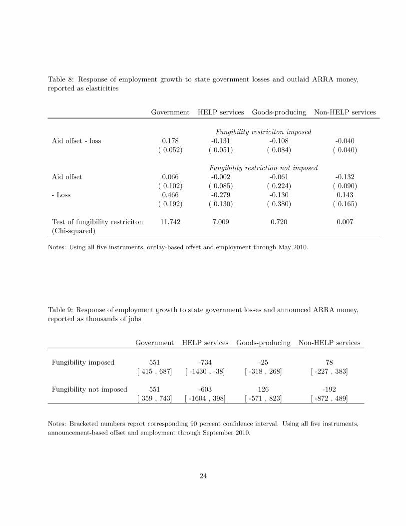
Table 8: Response of employment growth to state government losses and outlaid ARRA money,reported as elasticities

Government HELP services Goods-producing Non-HELP services

Fungibility restriciton imposedAid offset - loss 0.178 -0.131 -0.108 -0.040

( 0.052) ( 0.051) ( 0.084) ( 0.040)

Fungibility restriction not imposedAid offset 0.066 -0.002 -0.061 -0.132

( 0.102) ( 0.085) ( 0.224) ( 0.090)- Loss 0.466 -0.279 -0.130 0.143

( 0.192) ( 0.130) ( 0.380) ( 0.165)

Test of fungibility restriciton 11.742 7.009 0.720 0.007(Chi-squared)

Notes: Using all five instruments, outlay-based offset and employment through May 2010.

Table 9: Response of employment growth to state government losses and announced ARRA money,reported as thousands of jobs

Government HELP services Goods-producing Non-HELP services

Fungibility imposed 551 -734 -25 78[ 415 , 687] [ -1430 , -38] [ -318 , 268] [ -227 , 383]

Fungibility not imposed 551 -603 126 -192[ 359 , 743] [ -1604 , 398] [ -571 , 823] [ -872 , 489]

Notes: Bracketed numbers report corresponding 90 percent confidence interval. Using all five instruments,

announcement-based offset and employment through September 2010.

24

Table 10: Population-weighted results: Response of employment growth to state government lossesand outlaid ARRA money, reported as elasticities

Government HELP services Goods-producing Non-HELP services

Fungibility restriciton imposedAid offset - loss -0.054 -0.135 -0.332 -0.036

( 0.061) ( 0.039) ( 0.101) ( 0.028)

Fungibility restriction not imposedAid offset -0.086 -0.199 -0.583 -0.086

( 0.094) ( 0.067) ( 0.162) ( 0.052)- Loss 0.130 -0.065 0.051 0.074

( 0.136) ( 0.065) ( 0.281) ( 0.101)

Notes: Using all five instruments, ARRA outlay-based offset and employment through September 2010.

to give more weight to high population states. The error term for each state is multiplied by the

square root of that state’s population.

Why do this? Certainly, our statistical model assumes that the regression coefficients are the

same across states. Thus, strictly speaking there is no reason to give different weights to different

states’ error terms depending on the population of that state. Rather, our weighting scheme is an

expedient way to allow larger states to have a greater influence over coefficient estimates in case

there is some heterogeneity across states in the magnitude of the treatment effect. Alternatively,

policy makers may wish to assign greater relevance to a high population relative to a low population

state, e.g. California versus Rhode Island.

This change in the specification changes the estimates for the two service sectors very little

relatively to the benchmark. For the government sector, the employment effect becomes negative

rather than positive. For the goods-producing sector, the effect is negative as in the benchmark

but is much stronger. Using the population weights, all four sectors have a negative employment

effect.

Table 11 reports elasticities for ten alternative specifications. The pattern is clear. For all

but one specification, government employment is greater because of the Act. For all but one

specification, HELP services employment is lower because of the Act. Non-HELP services is close

to zero for each specification. The widest range of employment estimates occurs in the goods-

producing sector; however, in cases where it is positive, it is not statistically different from zero.

One natural question is: searching across all specifications in Table 11, what is the best-case

scenario for an effectual ARRA in terms of job creation? This is seen in row (vi), which impose

fungibility, use the benchmark specification except only use the sales tax intensity and highway

dollars instruments. In this case, the Act created a net 659 thousand jobs—the majority of which

25

Tab

le11

:R

esp

on

seof

emp

loym

ent

gro

wth

tost

ate

gove

rnm

ent

loss

esan

dA

RR

Am

oney

,m

isce

llan

eou

ssp

ecifi

cati

ons,

rep

orte

das

elas

tici

ties

Gov

ern

men

tH

EL

PS

ervic

esG

ood

sp

rod

uci

ng

Non

-HE

LP

Ser

vic

es

Pla

usi

ble

alt

ern

ati

vesp

ecifi

cati

on

s(i

)B

ench

mark

(fro

mta

ble

2)0.

139

-0.0

96-0

.106

0.01

3(

0.08

8)(

0.04

4)(

0.10

0)(

0.03

5)(i

i)D

rop

six

small

est

0.05

30.

166

-0.1

81-0

.033

(0.

088)

(0.

108)

(0.

133)

(0.

067)

(iii

)D

rop

six

larg

est

0.03

3-0

.121

-0.3

03-0

.024

(0.

077)

(0.

055)

(0.

099)

(0.

028)

(iv)

On

lypri

mar

yin

stru

men

ts0.

297

-0.1

260.

024

0.03

2(

0.09

9)(

0.08

3)(

0.10

2)(

0.04

4)(v

)K

eep

all

state

s0.

020

-0.1

03-0

.192

0.00

4(

0.08

0)(

0.05

1)(

0.09

1)(

0.02

8)

(vi)

Dro

psm

all

fou

ran

dN

V0.

240

-0.0

96-0

.024

0.02

1(

0.09

1)(

0.04

7)(

0.06

2)(

0.03

9)

Impla

usi

ble

spec

ifica

tion

s(f

or

com

pari

son

)(v

ii)

Dro

plo

ssre

gres

sor

0.16

0-0

.136

-0.2

030.

001

(0.

125)

(0.

064)

(0.

168)

(0.

046)

(vii

)D

rop

offse

tre

gre

ssor

0.36

5-0

.219

-0.0

920.

105

(0.

203)

(0.

123)

(0.

197)

(0.

130)

(ix)

Excl

ud

ere

gion

contr

ol0.

074

-0.1

370.

053

-0.0

24(

0.07

1)(

0.05

3)(

0.06

0)(

0.02

7)(x

)E

xcl

ud

ep

op

ula

tion

contr

ol0.

119

-0.0

97-0

.143

0.01

7(

0.09

0)(

0.04

5)(

0.12

9)(

0.03

4)

Not

es:

Em

plo

ym

ent

thro

ugh

Sep

tem

ber

2010

.In

ben

chm

ark

spec

ifica

tion

,th

efo

ur

low

est

pop

ula

tion

state

s(i

.e.

Ala

ska,

Nort

hD

ako

ta,

Ver

mon

tan

dW

yom

ing)

wer

eex

clu

ded

.T

he

two

pri

mary

inst

rum

ents

are

the

hig

hw

ayin

stru

men

tan

dsa

les

tax

inte

nsi

ty.

26

were in the government sector.

5 Other Researchers’ Estimates of Job Creation

Even before the legislation was passed, Bernstein and Romer (2009) reported that 3.6 million jobs

would be created or saved by the then envisioned legislation, relative to a no stimulus act baseline.

This was based on existing estimates of fiscal policy multipliers. Their estimates included both the

tax and spending components of the ARRA.

Congressional Budget Office (2010) estimates that the employment increase “attributable to the

ARRA” was in the range of 500 to 900 thousand in 2009 and is in the range of 1.3 to 3.3 million for

2010. Their ranges are computed based on both government spending as well as tax cut incentives

in the Act. To construct these numbers (in their Table 1), they divide the total spending of the

ARRA into its components and then apply low and high output multipliers. These multipliers were

delivered from previous studies.

The Council of Economic Advisors (2010) measures the employment increase due to the Act in

two different ways. First, using a multiplier approach similar to the Congressional Budget Office,

the CEA estimates that the Act had the effect of increasing employment by 2.5 million workers

(Table 4). Second, the CEA estimates a vector autoregression which includes employment from

1990:Q1 to 2007:Q4. Based on those parameter estimates, they forecast gross domestic product

for the period after the Act’s implementation. They then interpret the vector autoregression’s

forecast error for employment from 2009:Q2 to 2010:Q2 as being due to the policy. According to

these estimates (Table 5), at the end of 2010:Q2, the Act had increased employment by 3.6 million

workers.

Blinder and Zandi (2010) find that the employment increase due to the ARRA (including both

spending and tax cuts) was 2.7 million jobs. Their estimate is based on the Moody Analytics model

of the U.S. economy, which is a statistical model that includes restrictions based upon standard

Keynesian assumptions.

Wilson (2011) estimates the job effects of the Recovery Act using state-level variation in a

manner similar to ours. He instruments for endogenity using two cost estimates for the ARRA

that existed prior to the Act’s passage. He considers the effect on employment at different horizons

following the ARRA’s implementation. For employment through October 2010, he find that there

were 800 thousand additional jobs because of the stimulus. This is close to our “best case” scenario

for the ARRA described in the previous section.

While Wilson’s above number is relatively small compared to other studies, he does find larger

employment effects at a more short-run horizon. When evaluating the employment growth through

February rather than October of 2010, Wilson finds that the Act saved/created 2.3 million jobs.

Feyrer and Sacerdote (2011) conduct both a cross-sectional and time series analysis to estimate

the employment effects of the ARRA. Based on state-level data, their cross-section estimate implies

27

that the Act created/saved 1.9 million jobs, while their time series estimate implies that the Act

created/saved approximately 845 thousand jobs.37

The most crucial difference between their analysis and ours may be aggregation. In their

regressions, the jobs effect is restricted to be identical across employment sectors. Our modest

disaggregation into four sectors demonstrates that different sectors responded differently to ARRA

aid. First, we are able to reject statistically the hypothesis of identical sector responses. Sec-

ond, these differences are also quantitatively important. Third, the different trend behavior, over

the last decade, across sectors suggests different employment processes are at work. Finally, the

practical consideration that much aid flowed through state and local governments suggests that

government employment should be treated differently than private-sector employment. Also, dif-

ferences between our results and theirs might be explained by the differences in instruments; Feyrer

and Sacerdote (2011) use the average seniority of members of the U.S. House of Representations to

control for endogenity.

Cogan and Taylor (2010a) look at Bureau of Economic Analysis data on government purchases

of goods and services.38 They find that most government purchases occurred at the Federal rather

than state and local level and that these purchases account for only 2% of ARRA aid. They argue

that state and local governments did not make purchases of goods and services, but rather increased

transfer payments and reduced borrowing. As such, there was only a negligible impact of the Act

on aggregate output and employment. While our analysis confirms the fact that much funding

went through states, it is not clear whether wages and salaries of government workers are fully

or even partially captured by the National Income and Product Account measures of government

purchases.

6 Conclusion

Much work on the effects of the ARRA remains to be done. We found, surprisingly, either negligible

or negative effects of the Act on total employment; thus, it is important to explore whether alter-

native empirical specifications, besides the historical ‘Keynesian multiplier’ approach of Section 5

used by other researchers, are capable of finding a significant positive jobs effect.

The most promising avenue in this regard is to allow for cross-state positive spillovers. This

might result in estimates of a large positive jobs effect. Suppose, for example, that Georgia received

relatively more ARRA aid, which in turn stimulated that state’s economy. If, as a result, Georgia

residents’ vacation spending in Florida increased, then the increased vacationing might generate

jobs in Florida. Our methodology cannot pick up this effect.

37Feyrer and Sacerdote (2011) do not report results in units of employment; however, we can calculate this figurebased upon numbers they report: per capita stimulus is $1100, one job per $170,000 of stimulus (cross-section), onejob per $400,000 (time series). These statistics together with a U.S. population of 307 million imply the job totalsreported in the text.

38See also Cogan and Taylor (2010b).

28

If this type of spillover from interstate trade is widespread nationally, then the economy-wide

jobs effect of the ARRA may be actually larger than what we find. To address this, we are planning

to redo our analysis by adding time series variation to the current cross-state variation. Given data

collection lags and the fact that ARRA spending did not begin in earnest until mid-2009, we did

not have a sufficiently long time series to use this approach in the present paper.

Next, research on the ARRA, and in particular our empirical findings, demands greater struc-

tural economic modeling. In this study, we deliberately chose the relatively ‘model-free’ approach

for one of the first studies on this new government program and data set. The drawback is that,

at this point, we can only conjecture on the underlying, economic mechanisms that give rise to our

findings.

Equilibrium modeling, with specification of preferences, endowments and technologies, should

allow us to pinpoint these mechanisms. We predict that an accurate economic model of the ARRA

experience will have three essential features. First, the Great Recession and the Act’s implementa-

tion happened partway through a sectoral shift from goods-producing to a service (of a particular

type) sector economy as evidenced in Figure 2.39 Second, as explained in the paper, relatively less

educated people faced, and continue to face, a much worse job market than more educated people.

The way that state and local governments channeled ARRA funding into different sectors is likely

to have consequences for the effects of the Act. For this reason, an accurate model should differ-

entiate between high and low education workers along with their respective labor markets. Third,

we have provided substantial evidence that state and local governments have used part of ARRA

aid in a way not explicitly intended by Congress and the President. As such, an accurate model

of this period will include a hierarchal intergovernmental component in the spirit of Bradford and

Oates (1971a).

Acknowledgements

We are grateful to David Blau, Daniel Bunn, Gabriel Chodorow-Reich, Steve Cohen,

Jim Donlin, Duane Dupor, Paul Evans, Joel Gratz, Sam Gratz, Christian Hansen, Don

Haurin, Dough Hecox, Rabi Mishalani, Bahi Subhash, Bruce Weinberg, Mark Wolfgram,

Sara Vermillion, Matthew Yglesias as well as other academics and government officials for

useful conversations and background. We also thank seminar participants at the Federal

Reserve Bank of Cleveland and the Ohio State University. We are especially grateful to

Chris Robinson for assistance with Census data and Matt Lewis for his patience and counsel.

39Existing economic modeling of sectoral shifts include Davis and Haltiwanger (2001) and Phelan and Trejos (2000).

29

Appendix

Data Construction

ARRA outlaid dollars data are taken from the 13 August 2010 Federal agencies’ “Weekly

Financial and Activity Reports,” which are cumulative over time and available on the recov-

ery.gov web site.40 The Social Security Administration dollars are excluded entirely because

these are direct transfers paid by the Federal government to citizens. We also exclude

the following agencies from our data: General Services Administration, National Science

Foundation, Small Business Administration, Department of Interior, Federal Communica-

tion Commission, Department of State, Retirement Railroad Board, Department of Veterans

Administration, NASA. Each of these exclusions is due to one of the following reasons: data

was not reported in a useful manner, none of that agencies’ funding was reported as going

through the states. The total funding outlays from excluded agencies (expect for the SSA)

make up less than 2% of total ARRA outlays. Call this OUTLAY . Every variable, unless

otherwise noted, is indexed by state which we suppress for simplicity.

ARRA announced dollars are taken from the recovery.gov web site on 13 September 2010.

On the web site, these are reported as data summed across agencies for each state. The web

site states that some agencies’ data are not included here because these agencies did not

report announced dollars as broken down by state. Call this ANNOUNCE.

Next, we use the total tax revenue collected by state. This is collected by the U.S. Census

in the “Quarterly Summary of State and Local Government Tax Revenue,” which is available

on the Census web site.41 We construct annual total state tax collections from the quarterly

data. Call this STATETAXt, where t represents one year ending in June.42

Next, we need a measure of the pre-recession size of state revenue. Because we do not need

data since the recession’s beginning, we are able to use a more accurate measure of the size

of state government–one that includes non-tax state revenue sources. STATEREV ALLt

is the calendar-year state revenue from all sources, which is reported in the “Census of

Governments.”

In addition to state revenue, we will use state Medicaid outlays (independent of the

funding source). Medicaid data is available in National Association of State Budget Officers

(2009). There are two issues. First, unlike the quarterly census-collected tax revenue data,

the state-level NASBO Medicaid data is reported in annual, calendar amounts. Therefore,

we are unable to match Medicaid cost to the growth rate timing of state tax revenue ex-

40Documentation for the web site data is contained in Recovery Accountability and Transportation Board (2009)41Although the word ‘Local’ is in the title of the data series, in actuality the data does not report local tax

information.42Note that state tax is less than actual state government income. This is because we do not have up-to-date data

on the two main others sources of state income: earnings from other sources, e.g. university tuition, and non-ARRAFederal aid.

30

actly. Second, NASBO reports the 2009 Medicaid expenditures as an estimate only. Let

MEDICAIDt equal the annual spending in a state on Medicaid.

Using the above variables, we compute our outlay-based measure of ARRA aid relative

to the size of state government. Let

OFFSET =OUTLAY

1.75 × STATEREV ALL2008

In our robustness analysis, we estimate the model using OFFSET computed using the

ARRA announced rather than outlaid dollars.

OFFSETannounced =ANNOUNCE

1.75 × STATEREV ALL2008

Next, we compute a measure of fiscal stress faced by each state because of the recession.

We use the annualized decline in state tax revenue plus the increase in Medicaid costs. We

do so over seven quarters with the final quarter being 2010:Q3.

LOSS = − ∆T − ∆M

1.75 × STATREV ALL2008

where

∆T = 0.5×STATETAX2009+STATETAX2010+STATETAXAUTUMN2009 −1.75×STATETAX2008

∆M = 1.75 ×MEDICAID2009 − 1.75 ×MEDICAID2008

Employment is the non-farm payroll series, de-seasonalized, from the Bureau of Labor

Statistics Establishment Survey. This gives the number of workers in each state by month.

We use measures from four different sectors: government, HELP services, non-HELP services

and goods-producing. Each series has been deseasonalized either by us, using the Census’

X12 algorithm, or by the Census itself. Further details on the employment data appear in

the body of the paper.

We have five instruments. Our first is the ARRA dollars announced by the Federal High-

way Administration relative to state government revenue from all sources in 2008. Second,

“strong budget rules” is a dummy variable taking on one for a state that has relatively strin-

gent balanced budget requirements. This classification is taken from Table 2 of Clemens

and Miran (2010). Third, Democratic governor is a dummy variable constructed using the

Wikipedia entry “List of Current U.S. Governor” (extracted in July 2010). Fourth, the

31

spend-pay ratio gives the number of dollars spent by the Federal government in that state

relative to the Federal taxes paid by that state in 2005. It is from the Tax Foundation,

a private nonpartisan research group organization, and available at its web site taxfounda-

tion.org. Fifth, the intensity of sales tax usage is from the “Quarterly Summary of State

and Local Government Tax Revenue.” It measures the ratio of sales tax revenue relative to

all tax revenue in each state, averaged over 2007 through 2008.

The remaining data are exogenous variables used in estimation. Northeast, West and

Midwest are dummy variables based on the U.S. Census Bureau’s region definitions. Finally,

UI generosity reports the maximum weekly benefits amount from the 2010 U.S. Department

of Labor’s “Comparison of State UI Laws.” In the case that a maximum is reported as a

range in the report, we use the maximum from that range.

Partial Correlations

Table 12: Partial correlations of instruments on OFFSET and −LOSS

Offset - LossHighway dollar and percent sales tax instruments

Highway instrument 2.497 1.073Sales tax intensity 0.003 -0.063

All five instrumentsHighway instrument 2.774 1.043Sales tax intensity -0.036 -0.011Spent-pay ratio 0.036 -0.047Strong budget rule -0.009 0.020Democratic governor 0.017 0.010

Notes: Above are regression coefficients from the single-equation least-squares estimation of alternative

endogenous variables on instruments and all control variables.

32

References

American Recovery and Reinvestment Act, Public Law 111-5, 111th Congress, 17 February 2009.

Auerbach, A., W. Gale and B. Harris (2010), “Activist Fiscal Policy,” University of California-

Berkeley, working paper.

Barro, R. (2010), “The Stimulus Evidence One Year On,” Wall Street Journal Online, February

23.

Barro, R. and C. Redlick (2011), “Macroeconomic Effects of Government Purchases and Taxes,”

Quarterly Journal of Economics, forthcoming.

Bernstein, J. and C. Romer (2009), “The Job Impact of the American Recovery and Reinvestment

Plan,” Office of the Vice President-Elect, working paper.

Blanchard, O. and R. Perotti (2010), “An Empirical Characterization of the Dynamic Effects of

Changes in Government Spending and Taxes on Output,” Quarterly Journal of Economics 117,

1329-1368.

Blinder, A. and M. Zandi (2010), “How the Great Recession Was Brought to an End.”

Bradford, D. and W. Oates (1971a), “The Analysis of Revenue Sharing in a New Approach to

Collective Fiscal Decisions,” Quarterly Journal of Economics 85, pp. 416-439

Bradford, D. and W. Oates (1971b), “Towards a Predictive Theory of Intergovernmental Grants,”

American Economic Review 61, pp. 440-448

Boyd, D. and L. Dadayan (2010), “After Disasterous 2009, States Report Moderate Revenue

Growth in Early 2010,” State Revenue Report (July), Nelson A. Rockefeller Institute of Govern-

ment, University of Albany, State University of New York.

Clemens, J. and S. Miran (2010), “The Effects of State Budget Cuts on Employment and Income,”

Harvard University, working paper.

Cogan J. and J. Taylor (2010), “What the Government Purchases Multiplier Actually Multiplied

in the 2009 Stimulus Package,” NBER working paper 16505.

Cogan J. and J. Taylor (2010), “The Obama Stimulus Impact? Zero,” The Wall Street Journal,

December 7, pg. A23.

Congressional Budget Office (2010), “Estimated Impact of the American Recovery and Reinvest-

ment Act on Employment and Economic Output from April 2010 through June 2010,” CBO

Report, August.

33

Council of Economic Advisors (2010), “The Economic Impact of the American Recovery and

Reinvestment Act of 2009: Fourth Quarterly Report,” July 14.

Davis, S. and J. Haltiwanger (2001), “Sectoral Job Creation and Job Destruction in Response to

Oil Price Shocks,” Journal of Monetary Economics 48, pp. 465-512.

Deitz, R. A. Haughwout and C. Steindel(2010), “The Recession’s Impact on the State Budgets of

New York and New Jersey,” Current Issues in Economics and Finance 16 (June/July), Federal

Reserve Bank of New York.

Federal Highway Administration (2009), “American Recovery and Reinvestment Act of 2009 Im-

plementation Guidelines,” U.S. Department of Transportation, April 1 (updated).

Feyrer, J. and B. Sacerdote (2011), “Did the Stimulus Stimulate? Real Time Estimates of the

Effects of the American Recovery and Reinvestment Act,” NBER working paper 16759.

Frank, R. (2009), “Don’t Let the Stimulus Loose Its Spark,” The New York Times, August 23.

Greenfield, Stuart (2010), “Public Sector Employment: The Current Situation,” Center for State

and Local Government Excellence, working paper.

Hines, J. and R. Thaler (1995), “The Flypaper Effect,” Journal of Economic Perspectives 9, pp.

217-226.

Inman, Robert (2010), “States in Fiscal Distress,” NBER Working Paper 16086.

Kaiser Foundation (2010), “Medicaid and Managed Care: Key Data, Trends and Issues,” Policy

Brief 8046.

Knight, B. (2002), “Endogenous Federal Grants and Crowd-out of State Government Spending:

Theory and Evidence from the Federal Highway Aid Program,” American Economic Review, pp.

71-92.

Krugman, P. (2009), “Too Little of a Good Thing,” The New York Times, November 1.

Leeper, E., T. Walker and S. Yang (2009), “Fiscal Foresight and Information Flows,” Indiana

University, manuscript.

McNichol, E., P. Oliff and N. Johnson (2010a) “Recession Continues to Batter State Budgets;

State Responses Could Slow Recovery,” Center on Budget and Policy Priorities (updated July

15).

McNichol, E., P. Oliff and N. Johnson (2010b), “States Continue to Feel Recession’s Impact,”

Center on Budget and Policy Priorities (updated October 7).

34

Mertens, K. and M. Ravn (2009), “Empirical evidence on the aggregate effects of anticipated and

unanticipated US tax policy shocks,” CEPR Discussion Paper 7370.

Michigan Department of Transportation (2010), “2009 Comprehensive Annual Financial Report.”

Michigan Department of Transportation (2011), “2009-2010 Fiscal Year Letting Statistics.”

National Association of State Budget Officers, State Expenditure Report, various years.

Ohanian, L. (2009), “How Stimulating Is Stimulus?” Forbes.com, June 17.

State of New York (2009), “New York 2009-2010 Enacted Financial Report,” Division of the

Budget.

State of New York (2010), “New York 2010-2011 Enacted Financial Report,” Division of the Bud-

get.

Ohio Department of Transportation (2010), “Financial and Statistical Report: Fiscal Year 2009.”

Governor’s Office of the State of Ohio.

Phelan, C. and A. Trejos (2000), “The Aggregate Effects of Sectoral Reallocation,” Journal of

Monetary Economics 45, pp. 249-268.

Ramey, V. (2010), “Identifying Government Spending Shocks: It’s All in the Timing,” Quarterly

Journal of Economics.

The Recovery Accountability and Transparency Board (2009), “Recovery.gov: Download Center

Users Guide.”

Texas Department of Transportation (2009), “Annual Financial Report (unaudited).” Texas De-

partment of Transportation.

Texas Department of Transportation (2010), “Annual Financial Report (unaudited).” Texas De-

partment of Transportation.

U.S. Census Bureau (2009), “2008 Annual Surveys of State and Local Finances.”

U.S. Department of Education (2009), “Guidance: Funds under Title I, Part A of the Elemen-

tary and Secondary Education Act of 1965,” Office of Elementary and Secondary Education,

November (revised).

U.S. Department of Social Services (2010), “TANF Emergency Contingency Fund: American Re-

covery and Reinvestment Act (ARRA) of 2009,” PowerPoint presentation, November.

U.S. Department of Transportation (2010), “Recovery Act 1201 Maintenance of Effor Provision:

Preliminary Report on Implementation and Results,” November.

35

U.S. General Accountability Office (2009), “Planned Efforts and Challenges in Evaluating Compli-

ance with Maintenance of Effort Provisions,” GAO-10-247, November.

Washington Post (2009), “They’re Saying No to the Cash, but Talk Is Cheap,” March 15.

Wilson, D., “Fiscal Spending Multipliers: Evidence from the 2009 American Recovery and Rein-

vestment Act,” Federal Reserve Bank of San Fransico, working paper, 2010.

36