the all-electron gw method based on wien2k: implementation and applications
TRANSCRIPT

The all-electron GW method based on WIEN2k:Implementation and applications.
Ricardo I. Gomez-Abal
Fritz-Haber-Institut of the Max-Planck-SocietyFaradayweg 4-6, D-14195, Berlin, Germany
15th. WIEN2k-WorkshopMarch, 29th. 2008
R. Gomez-Abal (FHI-Berlin) GW@Wien2k Vienna 2008 1 / 54

Outline
Outline
1 Introduction
2 ImplementationGW@wien2kConvergence Tests
3 ResultsBandgapsBandstructuresMacroscopic Dielectric Constant
4 Core-valence interactionBandgapsSemicore States
5 f-electron systems
6 Conclusions
R. Gomez-Abal (FHI-Berlin) GW@Wien2k Vienna 2008 2 / 54
Introduction
Density Functional Theory
E ⇐⇒ ρ
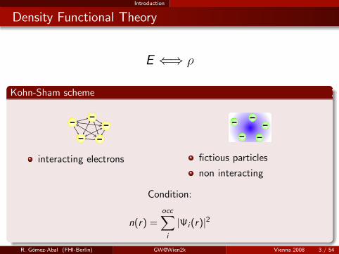
Kohn-Sham scheme
interacting electrons fictious particles
non interacting
Condition:
n(r) =
occ∑
i
|Ψi(r)|2
R. Gomez-Abal (FHI-Berlin) GW@Wien2k Vienna 2008 3 / 54
Introduction
Density Functional Theory
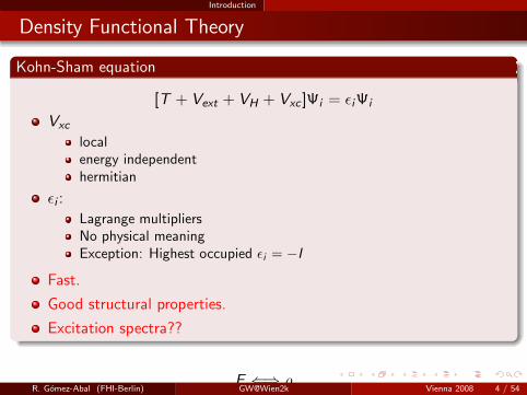
Kohn-Sham equation
[T + Vext + VH + Vxc ]Ψi = ǫiΨi
Vxc
localenergy independenthermitian
ǫi :
Lagrange multipliersNo physical meaningException: Highest occupied ǫi = −I
Fast.
Good structural properties.
Excitation spectra??
E ⇐⇒ ρR. Gomez-Abal (FHI-Berlin) GW@Wien2k Vienna 2008 4 / 54

Introduction
The Bandgap Problem
LDA vs. experimental bandgaps
Si
GaA
s
zGaN
ZnS
C
CaO M
gO
NaC
l
0 2 4 6 8Eg
exp [eV]
0
2
4
6
8E
gLDA [
eV]
Up to 50% underestimationR. Gomez-Abal (FHI-Berlin) GW@Wien2k Vienna 2008 5 / 54
Introduction
Many-Body Theory
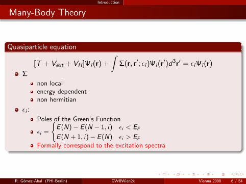
Quasiparticle equation
[T + Vext + VH ]Ψi (r) +
∫
Σ(r, r′; ǫi )Ψi (r′)d3r′ = ǫiΨi(r)
Σ
non localenergy dependentnon hermitian
ǫi :
Poles of the Green’s Function
ǫi =
E (N) − E (N − 1, i) ǫi < EF
E (N + 1, i) − E (N) ǫi > EF
Formally correspond to the excitation spectra
R. Gomez-Abal (FHI-Berlin) GW@Wien2k Vienna 2008 6 / 54

Introduction
Many Body Theory (cont.)
The Self-Energy (Σ)
Hedin, 1965: Expansion in terms of the dynamically screened Coulombpotential (W ).
Fast convergence.
First order:
Σ(r, t, r′, t ′) = G (r, t, r′, t ′)W (r, t, r′, t ′)
Simplest approximation including dynamical correlation effects
R. Gomez-Abal (FHI-Berlin) GW@Wien2k Vienna 2008 7 / 54
Introduction
Many Body Theory (cont.)
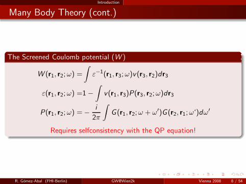
The Screened Coulomb potential (W )
W (r1, r2;ω) =
∫
ε−1(r1, r3;ω)v(r3, r2)dr3
ε(r1, r2;ω) =1 −∫
v(r1, r3)P(r3, r2;ω)dr3
P(r1, r2;ω) = − i
2π
∫
G (r1, r2;ω + ω′)G (r2, r1;ω‘)dω′
Requires selfconsistency with the QP equation!
R. Gomez-Abal (FHI-Berlin) GW@Wien2k Vienna 2008 8 / 54
Introduction
Perturbative treatment
G0W0
[T + Vext + VH ]Ψi (r)+∫
[
Σ(r, r′; ǫi)]
Ψi(r′)d3r′ = ǫiΨi(r)
R. Gomez-Abal (FHI-Berlin) GW@Wien2k Vienna 2008 9 / 54

Introduction
Perturbative treatment
G0W0
[T + Vext + VH + Vxc ]Ψi (r)+∫
[
Σ(r, r′; ǫi ) − Vxc(r′)δ(r − r′)
]
Ψi(r′)d3r′ = ǫiΨi(r)
R. Gomez-Abal (FHI-Berlin) GW@Wien2k Vienna 2008 9 / 54

Introduction
Perturbative treatment
G0W0
[T + Vext + VH + Vxc ]Ψi (r)+∫
[
Σ(r, r′; ǫi ) − Vxc(r′)δ(r − r′)
]
Ψi(r′)d3r′ = ǫiΨi(r)
R. Gomez-Abal (FHI-Berlin) GW@Wien2k Vienna 2008 9 / 54
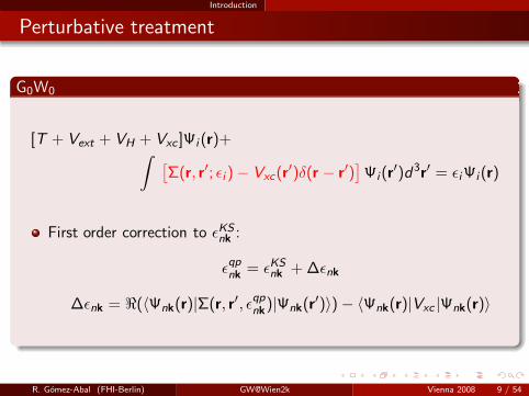
Introduction
Perturbative treatment
G0W0
[T + Vext + VH + Vxc ]Ψi (r)+∫
[
Σ(r, r′; ǫi ) − Vxc(r′)δ(r − r′)
]
Ψi(r′)d3r′ = ǫiΨi(r)
First order correction to ǫKSnk :
ǫqpnk = ǫKS
nk + ∆ǫnk
∆ǫnk = ℜ(〈Ψnk(r)|Σ(r, r′, ǫqpnk)|Ψnk(r
′)〉) − 〈Ψnk(r)|Vxc |Ψnk(r)〉
R. Gomez-Abal (FHI-Berlin) GW@Wien2k Vienna 2008 9 / 54
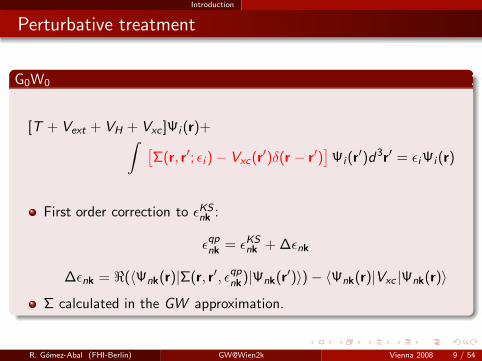
Introduction
Perturbative treatment
G0W0
[T + Vext + VH + Vxc ]Ψi (r)+∫
[
Σ(r, r′; ǫi ) − Vxc(r′)δ(r − r′)
]
Ψi(r′)d3r′ = ǫiΨi(r)
First order correction to ǫKSnk :
ǫqpnk = ǫKS
nk + ∆ǫnk
∆ǫnk = ℜ(〈Ψnk(r)|Σ(r, r′, ǫqpnk)|Ψnk(r
′)〉) − 〈Ψnk(r)|Vxc |Ψnk(r)〉Σ calculated in the GW approximation.
R. Gomez-Abal (FHI-Berlin) GW@Wien2k Vienna 2008 9 / 54

Introduction
Introduction
G0W0 equations
G0(r1, r2;ω) =occ∑
nk
Ψnk(r1)Ψ∗nk(r2)
ω − ǫnk − iη+
unocc∑
nk
Ψnk(r1)Ψ∗nk(r2)
ω − ǫnk + iη
P(r1, r2;ω) = − i
2π
∫
G0(r1, r2;ω + ω′)G0(r2, r1;ω‘)dω′
ε(r1, r2;ω) =1 −∫
v(r1, r3)P(r3, r2;ω)dr3
W0(r1, r2;ω) =
∫
ε−1(r1, r3;ω)v(r3, r2)dr3
Σ(r1, r2;ω) =i
2π
∫
G0(r1, r2;ω + ω′)W0(r2, r1;ω‘)dω′
R. Gomez-Abal (FHI-Berlin) GW@Wien2k Vienna 2008 10 / 54

Implementation GW@wien2k
Implementation
R. Gomez-Abal (FHI-Berlin) GW@Wien2k Vienna 2008 11 / 54

Implementation Basis Functions
The Polarization
P(r1, r2, ω) =X
n,m,k,k′
Ψnk(r1)Ψ∗
mk′(r1)Ψ∗
nk(r2)Ψmk′(r2)F(ǫnk, ǫmk′ ; ω)
R. Gomez-Abal (FHI-Berlin) GW@Wien2k Vienna 2008 12 / 54

Implementation Basis Functions
The basis functions
P(r1, r2, ω) =X
n,m,k,k′
Ψnk(r1)Ψ∗
mk′(r1)Ψ∗
nk(r2)Ψmk′(r2)F(ǫnk, ǫmk′ ; ω)
Definition
χqi (r) =
∑
Ra
e ik·(R+ra)υNL(r)YLM(r) r ∈ MT-spheres
1√V
∑
G
Si ,Ge i(q+G)·r r ∈ Interstitial
1 F. Aryasetiawan and O. Gunnarsson, Rep. Prog. Phys. 61, 237 (1998).
2 T. Kotani and M. van Schilfgaarde, Sol. State. Comm. 121, 461 (2002).
MTSphere
Interstitial
R. Gomez-Abal (FHI-Berlin) GW@Wien2k Vienna 2008 12 / 54

Implementation Basis Functions
The basis functions
Obtaining the radial functions
For each L take ul(r)ul ′(r) such that |l − l ′| ≤ L ≤ l + l ′
Calculate the overlap matrix:
Oall ′,l1l
′
1=
RMT∫
0
ul(r)ul ′(r)ul1(r)ul ′1(r)r2dr
Solve the secular equation:
(
Oall ′,l1l
′
1− λnδll1δl ′l ′1
)
cn,l1l′
1= 0
If λn ≥ λtol then:
υnL(r) =∑
ll ′
cn,ll ′ul (r)ul ′(r)
R. Gomez-Abal (FHI-Berlin) GW@Wien2k Vienna 2008 13 / 54
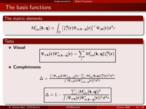
Implementation Basis Functions
The basis functions
The matrix elements
M inm(k,q) ≡
∫
Ω
[
χqi (r)Ψm,k−q(r)
]∗Ψnk(r)d
3r
Tests
Visual
Ψn,k(r)Ψ∗m,k−q(r) =
∑
i
M inm(k,q)χq
i (r)
Completeness
∆ =
R
|Ψn,k(r)Ψ∗
m,k−q(r)−
P
i Minm(k,q)χq
i(r)|2d3r
R
|Ψn,k(r)Ψ∗
m,k−q(r)|2d3r
∆ = 1 −∑
i |M inm(k,q)|2
∫
|Ψn,k(r)Ψ∗m,k−q(r)|2d3r
R. Gomez-Abal (FHI-Berlin) GW@Wien2k Vienna 2008 14 / 54

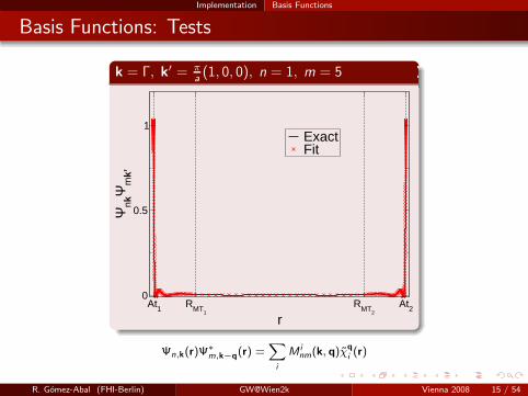
Implementation Basis Functions
Basis Functions: Tests
k = Γ, k′ = X , n = 4 m = 5
At1 RMT1RMT2
At2r
-0.04
-0.02
0
0.02
Ψnk
Ψm
k’ExactFit
Ψn,k(r)Ψ∗
m,k−q(r) =X
i
M inm(k, q)χq
i(r)
R. Gomez-Abal (FHI-Berlin) GW@Wien2k Vienna 2008 15 / 54

Implementation Basis Functions
Basis Functions: Tests
k = Γ, k′ = π
a(1, 0, 0), n = 2 m = 6
At1 RMT1RMT2
At2r
-0.01
0
0.01Ψ
nkΨ
mk’
ExactFit
Ψn,k(r)Ψ∗
m,k−q(r) =X
i
M inm(k, q)χq
i(r)
R. Gomez-Abal (FHI-Berlin) GW@Wien2k Vienna 2008 15 / 54

Implementation Basis Functions
Basis Functions: Tests
k = 3π
2a(1, 1,−1), k′ = π
2a(1,−1, 1), n = 2, m =
6
At1 RMT1RMT2
At2r
-0.1
-0.05
0
0.05
0.1Ψ
nkΨ
mk’
ExactFit
Ψn,k(r)Ψ∗
m,k−q(r) =X
i
M inm(k, q)χq
i(r)
R. Gomez-Abal (FHI-Berlin) GW@Wien2k Vienna 2008 15 / 54
Implementation Basis Functions
Basis Functions: Tests
k = Γ, k′ = π
a(1, 0, 0), n = 1, m = 5
At1 RMT1RMT2
At2r
0
0.5
1Ψ
nkΨ
mk’
ExactFit
Ψn,k(r)Ψ∗
m,k−q(r) =X
i
M inm(k, q)χq
i(r)
R. Gomez-Abal (FHI-Berlin) GW@Wien2k Vienna 2008 15 / 54
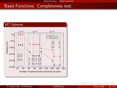
Implementation Basis Functions
Basis Functions: Completeness test.
MT-Spheres
20 40 60 80 100 120 140 160 180
Number of spherical basis functions per atom
1e-06
1e-05
1e-04
0.001
0.01
0.1
Rel
ativ
e er
ror
tol.
= 1
e-2
tol.
= 1
e-3
tol.
= 1
e-4
tol.
= 1
e-5
tol.
= 1
e-7
tol.
= 1
e-2
tol.
= 1
e-3
tol.
= 1
e-4
tol.
= 1
e-5
lmax=2 lmax=3lmax=1
tol.
= 1
e-2
tol.
= 1
e-3
tol.
= 1
e-5
MinimumMaximum
R. Gomez-Abal (FHI-Berlin) GW@Wien2k Vienna 2008 16 / 54
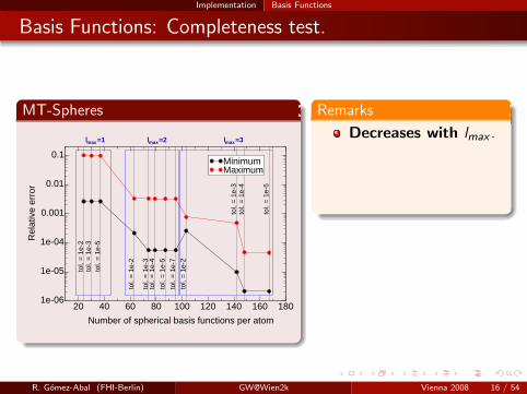
Implementation Basis Functions
Basis Functions: Completeness test.
MT-Spheres
20 40 60 80 100 120 140 160 180
Number of spherical basis functions per atom
1e-06
1e-05
1e-04
0.001
0.01
0.1
Rel
ativ
e er
ror
tol.
= 1
e-2
tol.
= 1
e-3
tol.
= 1
e-4
tol.
= 1
e-5
tol.
= 1
e-7
tol.
= 1
e-2
tol.
= 1
e-3
tol.
= 1
e-4
tol.
= 1
e-5
lmax=2 lmax=3lmax=1
tol.
= 1
e-2
tol.
= 1
e-3
tol.
= 1
e-5
MinimumMaximum
Remarks
Decreases with lmax .
Saturates with ǫtol
for a given lmax .
R. Gomez-Abal (FHI-Berlin) GW@Wien2k Vienna 2008 16 / 54

Implementation Basis Functions
Basis Functions: Completeness test.
Interstitial
150 200 250 300 350
Number of interstitial basis functions
1e-08
1e-07
1e-06
1e-05
1e-04
0.001
Rel
ativ
e er
ror
LAP
W b
asis
MinimumMaximum
Remarks
Decreases with lmax .
Saturates with ǫtol fora given lmax .
Decreases with
|Gmax |.
R. Gomez-Abal (FHI-Berlin) GW@Wien2k Vienna 2008 16 / 54

Implementation Basis Functions
Basis Functions: Completeness test.
Interstitial
150 200 250 300 350
Number of interstitial basis functions
1e-08
1e-07
1e-06
1e-05
1e-04
0.001
Rel
ativ
e er
ror
LAP
W b
asis
MinimumMaximum
Remarks
Decreases with lmax .
Saturates with ǫtol fora given lmax .
Decreases with |Gmax |.
Recipe
Choose max(ǫtol ) thatsaturates
Choose |Gmax | so that∆i ≈ ∆MT
R. Gomez-Abal (FHI-Berlin) GW@Wien2k Vienna 2008 16 / 54

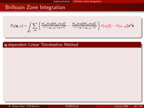
Implementation Brillouin Zone Integration
The Polarization
Pij(q, ω) =
Z
BZ
X
nm
M inm(k,q)[M j
nm(k,q)]∗
ω−ǫmk−q+ǫnk+iη−
M inm(k,q)[M j
nm(k,q)]∗
ω−ǫnk+ǫmk−q−iη
ff
f (ǫk)[1 − f (ǫk−q)]d3k
R. Gomez-Abal (FHI-Berlin) GW@Wien2k Vienna 2008 17 / 54

Implementation Brillouin Zone Integration
Brillouin Zone Integration
Pij(q, ω) =
Z
BZ
X
nm
M inm(k,q)[M j
nm(k,q)]∗
ω−ǫmk−q+ǫnk+iη−
M inm(k,q)[M j
nm(k,q)]∗
ω−ǫnk+ǫmk−q−iη
ff
f (ǫk)[1 − f (ǫk−q)]d3k
q-dependent Linear Tetrahedron Method
R. Gomez-Abal (FHI-Berlin) GW@Wien2k Vienna 2008 17 / 54

Implementation Brillouin Zone Integration
Brillouin Zone Integration
Pij(q, ω) =
Z
BZ
X
nm
M inm(k,q)[M j
nm(k,q)]∗
ω−ǫmk−q+ǫnk+iη−
M inm(k,q)[M j
nm(k,q)]∗
ω−ǫnk+ǫmk−q−iη
ff
f (ǫk)[1 − f (ǫk−q)]d3k
q-dependent Linear Tetrahedron Method
Linear Tetrahedron Method
P(q, ω) =
Z
BZ
X (k, q)f (ǫk)[1 − f (ǫk−q)]
ω − ∆ǫd
3k
wTki ,q
=
Z
ΩT
wi (k)f (ǫk)[1 − f (ǫk−q)]
ω − ∆ǫd
3k wki ,q =
X
T∋ki
wTki ,q
P(q, ω) =X
nm
X
i
X (ki , q)wnm(ki , q; ω)
J. Rath and A. J. Freeman, Phys. Rev. B 11, 2109 (1975)
R. Gomez-Abal (FHI-Berlin) GW@Wien2k Vienna 2008 17 / 54
Implementation Brillouin Zone Integration
Brillouin Zone Integration
Pij(q, ω) =
Z
BZ
X
nm
M inm(k,q)[M j
nm(k,q)]∗
ω−ǫmk−q+ǫnk+iη−
M inm(k,q)[M j
nm(k,q)]∗
ω−ǫnk+ǫmk−q−iη
ff
f (ǫk)[1 − f (ǫk−q)]d3k
q-dependent Linear Tetrahedron Method
R. Gomez-Abal (FHI-Berlin) GW@Wien2k Vienna 2008 18 / 54

Implementation Brillouin Zone Integration
Brillouin Zone Integration
Pij(q, ω) =
Z
BZ
X
nm
M inm(k,q)[M j
nm(k,q)]∗
ω−ǫmk−q+ǫnk+iη−
M inm(k,q)[M j
nm(k,q)]∗
ω−ǫnk+ǫmk−q−iη
ff
f (ǫk)[1 − f (ǫk−q)]d3k
q-dependent Linear Tetrahedron Method
~q
R. Gomez-Abal (FHI-Berlin) GW@Wien2k Vienna 2008 18 / 54
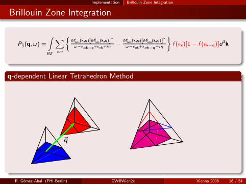
Implementation Brillouin Zone Integration
Brillouin Zone Integration
Pij(q, ω) =
Z
BZ
X
nm
M inm(k,q)[M j
nm(k,q)]∗
ω−ǫmk−q+ǫnk+iη−
M inm(k,q)[M j
nm(k,q)]∗
ω−ǫnk+ǫmk−q−iη
ff
f (ǫk)[1 − f (ǫk−q)]d3k
q-dependent Linear Tetrahedron Method
~q
R. Gomez-Abal (FHI-Berlin) GW@Wien2k Vienna 2008 18 / 54

Implementation Brillouin Zone Integration
Brillouin Zone Integration
Pij(q, ω) =
Z
BZ
X
nm
M inm(k,q)[M j
nm(k,q)]∗
ω−ǫmk−q+ǫnk+iη−
M inm(k,q)[M j
nm(k,q)]∗
ω−ǫnk+ǫmk−q−iη
ff
f (ǫk)[1 − f (ǫk−q)]d3k
q-dependent Linear Tetrahedron Method
R. Gomez-Abal (FHI-Berlin) GW@Wien2k Vienna 2008 19 / 54
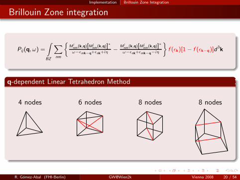
Implementation Brillouin Zone Integration
Brillouin Zone integration
Pij(q, ω) =
Z
BZ
X
nm
M inm(k,q)[M j
nm(k,q)]∗
ω−ǫmk−q+ǫnk+iη−
M inm(k,q)[M j
nm(k,q)]∗
ω−ǫnk+ǫmk−q−iη
ff
f (ǫk)[1 − f (ǫk−q)]d3k
q-dependent Linear Tetrahedron Method
4 nodes 6 nodes 8 nodes 8 nodes
R. Gomez-Abal (FHI-Berlin) GW@Wien2k Vienna 2008 20 / 54

Implementation Brillouin Zone Integration
q-dependent Linear Tetrahedron Method
Test: Free electron gas
0 0.5 1 1.5 2 2.5 3 3.5q/kF
0
0.2
0.4
0.6
0.8
1
Lind
hard
t fun
ctio
n
exact364 k-pts540 k-pts1368 k-pts
R. Gomez-Abal (FHI-Berlin) GW@Wien2k Vienna 2008 21 / 54

Implementation Brillouin Zone Integration
q-dependent Linear Tetrahedron Method
Test: Cu bandstructure
W L Γ X Z W K
-10
EF
10 LDAGW
R. Gomez-Abal (FHI-Berlin) GW@Wien2k Vienna 2008 22 / 54

Implementation Brillouin Zone Integration
q-dependent Linear Tetrahedron Method
Test: Cu DOS
-8 -6 -4 -2 EF2 4
Energy [eV]
0
1
2
3
4
5
6D
OS
LDAGW
R. Gomez-Abal (FHI-Berlin) GW@Wien2k Vienna 2008 23 / 54
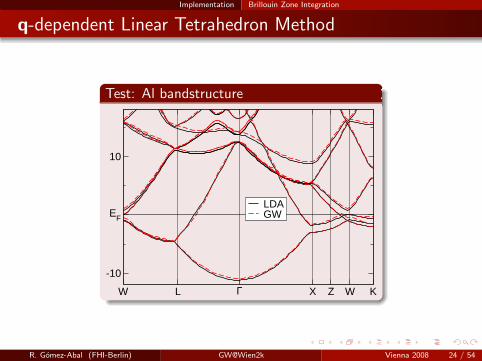
Implementation Brillouin Zone Integration
q-dependent Linear Tetrahedron Method
Test: Al bandstructure
W L Γ X Z W K
-10
EF
10
LDAGW
R. Gomez-Abal (FHI-Berlin) GW@Wien2k Vienna 2008 24 / 54

Implementation The Γ-point singularity
The Γ point singularity
The symmetrized dielectric matrix
Definition
εij (q, ω) =∑
lm
v12il (q)Plm(q, ω)v
12mj (q)
The screened potential
Wij(q, ω) =∑
lm
v12il (q)ε−1
lm (q, ω)v12mj (q)
R. Gomez-Abal (FHI-Berlin) GW@Wien2k Vienna 2008 25 / 54

Implementation The Γ-point singularity
The Γ point singularity
The screened Coulomb potential
v12
ij (q → 0) =v
s 12
ij
|q|+ v
12
ij (q)
Wij(q, ω) =1
|q|2W s2
ij (q, ω) +1
|q|W s1
ij (q, ω) + Wij(q, ω)
Diverges!
R. Gomez-Abal (FHI-Berlin) GW@Wien2k Vienna 2008 26 / 54

Implementation The Γ-point singularity
The Γ point singularity
The screened Coulomb potential
v12
ij (q → 0) =v
s 12
ij
|q|+ v
12
ij (q)
Wij(q, ω) =1
|q|2W s2
ij (q, ω) +1
|q|W s1
ij (q, ω) + Wij(q, ω)
But can be integrated
R. Gomez-Abal (FHI-Berlin) GW@Wien2k Vienna 2008 26 / 54

Implementation Frequency convolution
Implementation
Frequency convolution
Σ(r1, r2; ω) =i
2π
Z
G0(r1, r2; ω + ω′)W0(r2, r1; ω‘)dω
′
⇓ Analytic continuation
Σ(r1, r2; iω) =i
2π
Z
G0(r1, r2; iω + iω′)W0(r2, r1; iω‘)diω
′
R. Gomez-Abal (FHI-Berlin) GW@Wien2k Vienna 2008 27 / 54

Implementation Frequency convolution
Implementation
Frequency convolution
Σ(r1, r2; ω) =i
2π
Z
G0(r1, r2; ω + ω′)W0(r2, r1; ω‘)dω
′
⇓ Analytic continuation
Σ(r1, r2; iω) =i
2π
Z
G0(r1, r2; iω + iω′)W0(r2, r1; iω‘)diω
′
Σnk(iω) = −X
q
X
ij
X
n′
M inn′ (k, q)
1
π
∞Z
0
Wij (q; iω′)dω′
(iω − ǫn,k′)2 + ω′2M
∗j
n′n(k, q)
Pade Approximant
Σnk(iω) =
PN
j=0 aj(iω)j
PN+1j=0 bj(iω)j
⇓ Analytic continuation
Σnk(ω) =
PN
j=0 ajωj
PN+1j=0 bjω
j
R. Gomez-Abal (FHI-Berlin) GW@Wien2k Vienna 2008 27 / 54

Implementation Summary
G0W0@Wien2k: A FP-(L)APW+lo + G0W0 code
Flowchart
Wien2k Begin
ψkn χiq
ǫDFTkn M i
nm(k, q) vij (q)
Pij (q, ω)
εij (q, ω)
Wij (q, ω)
V xck,n Σnn(k, ω)
ǫqpk,n
End
Code keywords
Based on FP-(L)APW+lo
Mixed Basis
Linear TetrahedronMethod
Reciprocal space
Imaginary frequencies
Excelent results
R. Gomez-Abal (FHI-Berlin) GW@Wien2k Vienna 2008 28 / 54

Implementation Convergence Tests
Silicon: Convergence tests
Number of frequencies
10 15 20 25Nr. of frequencies
0.878
0.879
0.88
0.881
0.882
0.883
0.884
Eg [e
V]
Used paremeters
16 frequencies
R. Gomez-Abal (FHI-Berlin) GW@Wien2k Vienna 2008 29 / 54

Implementation Convergence Tests
Silicon: Convergence tests
Number of excited states
8 27 64 125Nr. of k-points
0.45
0.46
0.47
0.48
0.49
0.5
0.51
0.52
0.53
∆Eg [e
V]
Used paremeters
16 frequencies
64 k-points
R. Gomez-Abal (FHI-Berlin) GW@Wien2k Vienna 2008 29 / 54

Implementation Convergence Tests
Silicon: Convergence tests
Number of k-points
0 50 100 150 200 250Number of unoccupied bands
0.95
1
1.05
1.1
Ban
d G
ap
Used paremeters
16 frequencies
64 k-points
∼ 200 unocc. bands
R. Gomez-Abal (FHI-Berlin) GW@Wien2k Vienna 2008 29 / 54

Results Bandgaps
Results I:
BandgapsS
i GaA
s
zGaN Z
nS
C
MgO
NaC
l
CaO
0 2 4 6 8Experimental Eg [eV]
0
2
4
6
8
10
Cal
cula
ted
Eg [e
V]
G0W0 All electronG0W0 PseudopotentialsG0W0@Wien2kLDA
- F. Aryasetiawan and O.Gunnarson, Rep. Prog. Phys.61, 237 (1998).(and Refs.)
- T. Kotani and M. vanSchilfgaarde, Solid State Comm.121, 461 (2002).
- C. Friedrich et al, Phys. Rev. B74, 045104 (2006).
R. Gomez-Abal (FHI-Berlin) GW@Wien2k Vienna 2008 30 / 54
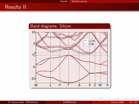
Results Bandstructures
Results II:
Band diagrams: Silicon
W ΓL Λ ∆ X Z W K
-10
-5
εF
5
10
1
LDAGW
R. Gomez-Abal (FHI-Berlin) GW@Wien2k Vienna 2008 31 / 54

Core-valence interaction Motivation
Motivation
G0W0 Si bandgap
1990 2000Publication year
0
0.5
1
1.5
Eg [e
V]
PseudopotentialsAll electron
R. Gomez-Abal (FHI-Berlin) GW@Wien2k Vienna 2008 32 / 54

Core-valence interaction Motivation
Motivation
G0W0 Si bandgap
1990 2000Publication year
0
0.5
1
1.5
Eg [e
V]
PseudopotentialsAll electron
R. Gomez-Abal (FHI-Berlin) GW@Wien2k Vienna 2008 32 / 54

Core-valence interaction Motivation
Debate
G0W0 Si bandgap
1990 2000 2010Publication year
0
0.5
1
1.5
Eg [e
V]
PseudopotentialsAll electron
?
- M. Tiago et al, Phys. Rev. B 69, 125212 (2004).
- C. Friedrich et al, Phys. Rev. B 74, 045104 (2006).
Pseudopotentials
systematically largergaps
in better agreementwith expeeriment
All electron
Benchmark for ab-initio
calculations
- A. Fleszar, Phys. Rev. B 64, 245204(2001).
- T. Kotani and M. van Schilfgaarde,Solid State Comm. 121, 461 (2002).
- W. Ku and A. Eguiluz, Phys. Rev. Lett.89,126401 (2002).
R. Gomez-Abal (FHI-Berlin) GW@Wien2k Vienna 2008 33 / 54

Core-valence interaction Core-valence Partitioning
Core-valence partitioning
Kohn-Sham equation
HKSΨnk = ǫnkΨnk
All electron
HKS = T + Vnuc + Vh + Vxc [n]
Pseudopotentials
HKS = T + Vps + Vh + Vxc [nv + nc ]
Vxc [n] = Vxc [nv + nc ] + Vxc [ncore − nc ] ⊂ Veff
G0W0 correctionǫqpnk = ǫKS
nk + ∆ǫnk
All electron
∆ǫnk = ℜ (Σnk [Ψnk; Ψc])− V xcnk [n]
Pseudopotentials
∆ǫnk = ℜ(Σnk[Ψnk])−V xcnk [nv +nc ]
ℜ (Σnk [Ψnk; Ψc]) = ℜ(Σnk[Ψnk]) + V xcnk [ncore − nc ] ⊂ Veff
R. Gomez-Abal (FHI-Berlin) GW@Wien2k Vienna 2008 34 / 54

Core-valence interaction Different Approaches
Different Approaches
G0W0 correction
All electron:
ǫqpnk = ǫKS
nk + ℜ (Σnk [Ψnk; Ψcore]) − V xcnk [n]
Pseudopotentials:
ǫqpnk = ǫKS
nk + ℜ(Σnk[Ψnk]) − V xcnk [nval ]
Valence only:
ǫqpnk = ǫKS
nk + ℜ (Σnk [Ψnk]) − V xcnk [nval ]
Separated terms
Σnk = Σxnk + Σc
nk
R. Gomez-Abal (FHI-Berlin) GW@Wien2k Vienna 2008 35 / 54
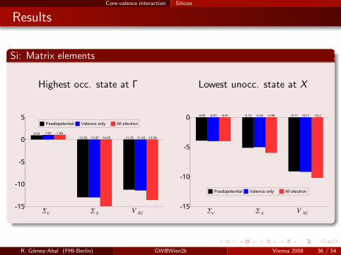
Core-valence interaction Silicon
Results
Si: Matrix elements
Highest occ. state at Γ
-15
-10
-5
0
5
0.93
-12.95 -11.25
1.03
-12.97 -11.43
1.05
-14.95 -13.54
Psedopotential Valence only All electron
C
XVXC
Lowest unocc. state at X
-15
-10
-5
0 -3.93 -5.13 -9.11-4.01 -5.03 -9.17-4.01 -5.98 -10.2
Psedopotential Valence only All electron
C
XVXC
R. Gomez-Abal (FHI-Berlin) GW@Wien2k Vienna 2008 36 / 54
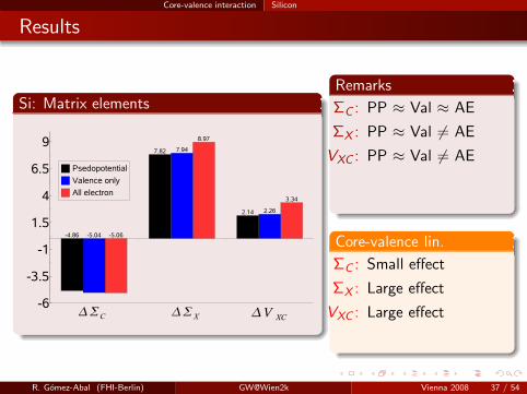
Core-valence interaction Silicon
Results
Si: Matrix elements
-6
-3.5
-1
1.5
4
6.5
9
-4.86
7.82
2.14
-5.04
7.94
2.26
-5.06
8.97
3.34
Psedopotential
Valence only
All electron
C
X VXC
Remarks
ΣC : PP ≈ Val ≈ AE
ΣX : PP ≈ Val 6= AE
VXC : PP ≈ Val 6= AE
Core-valence lin.
ΣC : Small effect
ΣX : Large effect
VXC : Large effect
R. Gomez-Abal (FHI-Berlin) GW@Wien2k Vienna 2008 37 / 54
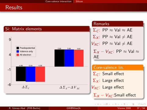
Core-valence interaction Silicon
Results
Si: Matrix elements
-6
-1
4
9
-4.86
5.68
-5.04
5.68
-5.06
5.63Psedopotential
Valence only
All electron
C
XV
XC
Remarks
ΣC : PP ≈ Val ≈ AE
ΣX : PP ≈ Val 6= AE
VXC : PP ≈ Val 6= AE
ΣX − VXC : PP ≈ Val ≈AE
Core-valence lin.
ΣC : Small effect
ΣX : Large effect
VXC : Large effect
ΣX − VXC :Small effect
R. Gomez-Abal (FHI-Berlin) GW@Wien2k Vienna 2008 37 / 54
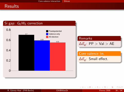
Core-valence interaction Silicon
Results
Si gap: G0W0 correction
0
0.2
0.4
0.6
0.8
0.7
0.59
0.55
Psedopotential
Valence only
All electronRemarks
∆Eg : PP > Val > AE
Core-valence lin.
∆Eg : Small effect.
R. Gomez-Abal (FHI-Berlin) GW@Wien2k Vienna 2008 38 / 54

Core-valence interaction GaAs
Results
GaAs: Matrix elements
Highest occ. state at Γ
-17.5
-15
-12.5
-10
-7.5
-5
-2.5
0
2.51.25
-12.86 -11.25
1.16
-12.5 -11.43
1.65
-17.17 -15.67
Psedopotential
Valence only
All electron
C
XVXC
Lowest unocc. state at Γ
-17.5
-15
-12.5
-10
-7.5
-5
-2.5
0 -3.55 -6.53 -10.34-3.21 -6.71 -10.67-3.58 -11.77 -16.7
Psedopotential
Valence only
All electron
C
XVXC
R. Gomez-Abal (FHI-Berlin) GW@Wien2k Vienna 2008 39 / 54

Core-valence interaction GaAs
Results
GaAs: Matrix elements
-7.5
-5
-2.5
0
2.5
5
7.5
-4.8
6.23
0.91
-4.37
5.79
0.76
-5.23
6
-1.03
Psedopotential
Valence only
All electron
C
X VXC
Remarks
ΣC : PP ≈ Val ≈ AE
ΣX : PP ≈ Val 6= AE
VXC : PP ≈ Val 6= AE
Core-valence lin.
ΣC : Small effect
ΣX : Large effect
VXC : Large effect
R. Gomez-Abal (FHI-Berlin) GW@Wien2k Vienna 2008 40 / 54

Core-valence interaction GaAs
Results
GaAs: Matrix elements
-7.5
-5
-2.5
0
2.5
5
7.5
-4.8
5.32
-4.37
5.03
-5.23
6.43
Psedopotential
Valence only
All electron
C
XV
XC
Remarks
ΣC : PP ≈ Val ≈ AE
ΣX : PP ≈ Val 6= AE
VXC : PP ≈ Val 6= AE
ΣX − VXC : PP ≈ Val 6=AE
Core-valence lin.
ΣC : Small effect
ΣX : Large effect
VXC : Large effect
ΣX − VXC :Large effect
R. Gomez-Abal (FHI-Berlin) GW@Wien2k Vienna 2008 40 / 54

Core-valence interaction GaAs
Results
GaAs gap: G0W0 correction
0
0.25
0.5
0.75
1
1.25
0.630.66
1.2
Psedopotential
Valence only
All electron
Remarks
∆Eg : PP < Val < AE
Core-valence lin.
∆Eg : Large effect.Reduces the correction!!
R. Gomez-Abal (FHI-Berlin) GW@Wien2k Vienna 2008 41 / 54

Core-valence interaction GaAs
Conclusions
C Si BN AlP GaAs LiF NaCl CaSe-0.6
-0.4
-0.2
0
0.2
0.4
0.6core-valence partitioning
pseudoization
Core-valence partitioning:
Strong changes in ΣX and VXC
Small changes in ΣC
∆Eg : Small changes in Si. Large in GaAsDoes NOT systematically increase the G0W0-correction.
“Pseudoization” also plays an important role.
R. Gomez-Abal (FHI-Berlin) GW@Wien2k Vienna 2008 42 / 54

Core-valence interaction Semicore States
Semicore states
Semicore states binding energies
MgO 6p-5p1s transition energy
TotalW L Λ Γ ∆ X ZW K-50
-40
-30
-20
-10
EF
10
Ene
rgy
[eV
]
sMg pMg s0 pO
LDA
:= 4
3.55
eV
GW
:= 5
2.41
eV
Excitation energy [eV]
ROHF(∆SCF)1 54.6CASTP21 53.8LDA2 43.5G0W
20 52.4
Experiment3 53.4
1.- C. Sousa et al. Phys. Rev. B 62,10013 (2000).2.- This work.3.- W. L. OBrien et al. Phys. Rev. B
44, 1013 (1991).
R. Gomez-Abal (FHI-Berlin) GW@Wien2k Vienna 2008 43 / 54

f-electron systems
f-electron systems
Motivation
Two strongly interrelated subsystems
itinerant spd statesstrongly localized f states
Intriguing physics
Heavy fermionKondo effectEtc...
Challenge to first-principle calculations:
LDA/GGA good for itinerant electronsFails for f -electrons
R. Gomez-Abal (FHI-Berlin) GW@Wien2k Vienna 2008 44 / 54

f-electron systems
(no)f-electron systems
CeO2
-6 -4 -2 0 2 4 6 8 10 12Energy [eV]
0
5
10
15
DO
SLDALDA-G0W0
XPS+BISXPS+XAS
E. Wuilloud et al. Phys. Rev. Lett 53, 202 (1984)
D. R. Mullins et al. Surf. Sci. 409, 307 (1998)
R. Gomez-Abal (FHI-Berlin) GW@Wien2k Vienna 2008 45 / 54

f-electron systems
(no)f-electron systems
Bandgaps
ZrO2 HfO2 CeO2 p-f
CeO2 p-d
ThO2
0
1
2
3
4
5
6
7E
g [eV
]LDAG0W0Expt.
R. Gomez-Abal (FHI-Berlin) GW@Wien2k Vienna 2008 46 / 54

f-electron systems
f-electron systems
Ce2O3
-10 -8 -6 -4 -2 0 2 4 6 8 10Energy [eV]
0
5
10D
OS
Expt.LDA
XPS XAS
E. Wuilloud et al. Phys. Rev. Lett 53, 202 (1984)
R. Gomez-Abal (FHI-Berlin) GW@Wien2k Vienna 2008 47 / 54

f-electron systems
f-electron systems
Ce2O3
-10 -8 -6 -4 -2 0 2 4 6 8 10Energy [eV]
0
5
10D
OS
Expt.LDALDA+U
XPS XAS
E. Wuilloud et al. Phys. Rev. Lett 53, 202 (1984)
R. Gomez-Abal (FHI-Berlin) GW@Wien2k Vienna 2008 47 / 54

f-electron systems
f-electron systems
Ce2O3
-10 -8 -6 -4 -2 0 2 4 6 8 10Energy [eV]
0
5
10D
OS
Expt.LDALDA+ULDA+U+G0W0
XPS XAS
E. Wuilloud et al. Phys. Rev. Lett 53, 202 (1984)
R. Gomez-Abal (FHI-Berlin) GW@Wien2k Vienna 2008 47 / 54

f-electron systems
f-electron systems
Bandgaps
La2O3 Ce2O3 Pr2O3 Nd2O30
1
2
3
4
5
6E
g [e
V]
Expt.LDA+UG0W0
R. Gomez-Abal (FHI-Berlin) GW@Wien2k Vienna 2008 48 / 54
Conclusions
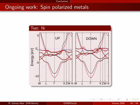
Ongoing work: Spin polarized metals
Test: Ni
W L Γ X ZW K
-10
-5
EF
5E
nerg
y [e
V]
W L Γ X ZW K
UP DOWN
R. Gomez-Abal (FHI-Berlin) GW@Wien2k Vienna 2008 49 / 54

Conclusions
Conclusions
GW@Wien2k
Reliable results.
Wide range of materials.
sp semiconductorsf -electron systems with empty or full f -shellsmetalsspin polarized materials
LDA+U+G0W0
R. Gomez-Abal (FHI-Berlin) GW@Wien2k Vienna 2008 50 / 54

Conclusions
Conclusions
Most important
R. Gomez-Abal (FHI-Berlin) GW@Wien2k Vienna 2008 51 / 54

Conclusions
Conclusions
Most important
Now we are enjoying it!!!
R. Gomez-Abal (FHI-Berlin) GW@Wien2k Vienna 2008 51 / 54
Conclusions
Last but not least
Future plans
Anisotropy of εmacro
Half metals
Efficiency Improvement
COHSEX@Wien2k + GW
BSE
QPscGW
R. Gomez-Abal (FHI-Berlin) GW@Wien2k Vienna 2008 52 / 54

Conclusions
Acknowledgements
Xinzheng Li (FHI, Berlin): Code development, LTM library.
Dr. Hong Jiang (FHI, Berlin): Code improvement, Spin polarization,LDA+U.
Prof. Claudia Ambrosch-Draxl (MUL; Austria): Wien2k interface andmore...
Christian Meisenbichler (MUL; Austria): MPI Paralelization
Patrick Rinke and Christoph Freysoldt (FHI, Berlin):Pseudopotentials, etc..
The boss
Matthias Scheffler
R. Gomez-Abal (FHI-Berlin) GW@Wien2k Vienna 2008 53 / 54