the advantage system: performance update

CONTACT

Corporate Headquarters3033 Beta AveBurnaby, BC V5G 4M9CanadaTel. 604-630-1428

US O�ce2650 E Bayshore RdPalo Alto, CA 94303

Email: [email protected]

www.dwavesys.com

Overview

This report presents a high-level overview of the Advantage™ quantumcomputing system. Advantage quantum processing units (QPUs) canhold application inputs that are almost three times larger, on average,than those that �t on previous-generation D-Wave 2000Q™ QPUs.Beyond the capacity to read bigger problems, comparison of an Ad-vantage performance update (herein referred to as Advantage 4.1) toa D-Wave 2000Q solver demonstrates that Advantage systems candeliver signi�cantly better performance on application-relevant inputs.The Advantage 4.1 solver also outperforms the original Advantage 1.1solver launched in 2020. We attribute this improved performance toinnovations in chip design as well as new fabrication materials and pro-cesses.

The Advantage System: Performance Update

TECHNICAL REPORT

Catherine McGeoch and Pau Farré

2021-10-01

14-1054A-AD-Wave Technical Report Series

Advantage Update i

Notice and DisclaimerD-Wave Systems Inc. (“D-Wave”) reserves its intellectual property rights in and to this doc-ument, any documents referenced herein, and its proprietary technology, including copyright,trademark rights, industrial design rights, and patent rights. D-Wave trademarks used hereininclude D-WAVE®, Leap™ quantum cloud service, Ocean™, Advantage™ quantum system,D-Wave 2000Q™, D-Wave 2X™, and the D-Wave logo (the “D-Wave Marks”). Other marks used inthis document are the property of their respective owners. D-Wave does not grant any license, assign-ment, or other grant of interest in or to the copyright of this document or any referenced documents,the D-Wave Marks, any other marks used in this document, or any other intellectual property rightsused or referred to herein, except as D-Wave may expressly provide in a written agreement.

Copyright © D-Wave Systems Inc.

Advantage Update ii

SummaryThis report presents a high-level overview of D-Wave’s Advantage™ quantum computingsystem. This is an updated version of a report published with the launch of the Advan-tage product line in September 2020; it contains new performance data for an Advantageperformance update made publicly available in October 2021.

Technological advances in the design of the quantum processing unit (QPU) at its coremake Advantage processors by far the largest and most powerful quantum computers inexistence today:

• Every Advantage processor contains at least 5,000 qubits, about 2.5 times more thanfound in a D-Wave 2000Q processor. The number of couplers per qubit has increasedfrom 6 to 15, for a total of at least 35,000 couplers, representing about a six-fold in-crease over the earlier system.

• More qubits and couplers means that larger application problems can be solved di-rectly on Advantage QPUs. An Advantage QPU can hold inputs between 2 and 5times larger than similarly-structured inputs that fit on a D-Wave 2000Q QPU, about3 times larger on average.

• More couplers per qubit means that application problems can be mapped more com-pactly onto the Advantage QPU. Compactness is measured by chain length: chainson Advantage QPUs are typically less than half as long as chains on D-Wave 2000QQPUs.

Beyond the capacity to read and solve larger inputs, Advantage processors can find better-quality solutions than 2000Q processors. This report compares the Advantage performanceupdate (herein referred to as Advantage 4.1) to a previous-generation D-Wave 2000Q solver(referred to as 2000Q), in terms of their physical properties and quality of solutions re-turned, in tests using application-relevant inputs. Key findings are summarized below.

• On clique problems, the Advantage 4.1 solver found optimal solutions on inputs thatwere 62 percent larger than the largest optimally-solved inputs on the 2000Q solver.In cases where both found optimal solutions, Advantage 4.1 found them faster, upto 54 times faster in terms of pure anneal time, or about 14 times faster in wall-clocktime. Overall, the Advantage 4.1 system found better solutions on 53 percent of in-puts, over 16 times more often than the 2000Q system, which won on just 3 percentof inputs (the remaining 44 percent of cases were ties).

• On inputs for the NAE3SAT problem, Advantage 4.1 again outperformed the 2000Q.In one test, the Advantage 4.1 QPU found better solutions on 81 percent of inputs,compared to just 0.9 percent of inputs for the 2000Q QPU (about 90 times more often).

• On inputs for 3D lattice problems, the Advantage 4.1 QPU found optimal solutionsup to 10 times faster than the 2000Q QPU, considering pure anneal times.

• Comparison data for the original Advantage system launched in September 2020 ap-pears in Appendix A: The Advantage 4.1 solver outperforms its predecessor (Advan-tage 1.1) in nearly every metric considered in this report. We attribute this improved


Advantage Update iii

performance to innovations in chip design as well as new fabrication materials andprocesses.

The report also shows how software tools from the Ocean developers toolkit can be usedto improve raw QPU outputs. This type of hybrid strategy combining the best features ofquantum and classical computation can often produce better results than either approachalone.


Advantage Update iv

Contents1 Introduction 1

2 New Advantage Features 32.1 More Compact Embeddings . . . . . . . . . . . . . . . . . . . . . . . . . . . . . 42.2 Bigger Inputs, Shorter Chains . . . . . . . . . . . . . . . . . . . . . . . . . . . . 62.3 Chain Length and Chain Strength . . . . . . . . . . . . . . . . . . . . . . . . . . 8

3 Performance Comparison 93.1 Hardware and Software Better Together . . . . . . . . . . . . . . . . . . . . . . 103.2 Performance Analysis . . . . . . . . . . . . . . . . . . . . . . . . . . . . . . . . . 12

4 Conclusions 17

References 18


Advantage Update 1

1 IntroductionThis report presents a high-level overview of the Advantage™ quantum system. The quan-tum processing unit (QPU) at its core represents a new pinnacle of design innovation andtechnological advances brought about by D-Wave engineers and scientists. Advantage isby far the largest and most powerful quantum computer in existence today.

This is an updated version of a technical report that was published concurrently with thelaunch of the Advantage generation of quantum processors in September 2020. This ver-sion contains new performance data from an Advantage performance update made pub-licly available in October 2021.

Throughout this report, a reference to “the Advantage QPU” or “the D-Wave 2000Q sys-tem” applies generally to solvers in those respective product lines. Sections describing em-pirical results refer to specific solvers used in those tests: the Advantage performance up-date is herein referred to as Advantage 4.1; the original Advantage processor launched in2020 is Advantage 1.1; and a specific D-Wave 2000Q LN (lower noise) solver released in2019 is referred to as the 2000Q.1

Section 2 gives an overview of the main design features of the Advantage generation ofquantum processors, in comparison to its predecessor the D-Wave 2000Q system. Section3 presents a brief performance comparison of two specific solvers known as Advantage4.1 and 2000Q. (Comparisons to the Advantage 1.1 solver may be found in Appendix A.)Section 4 contains some final remarks.

The key results in this report are summarized below.

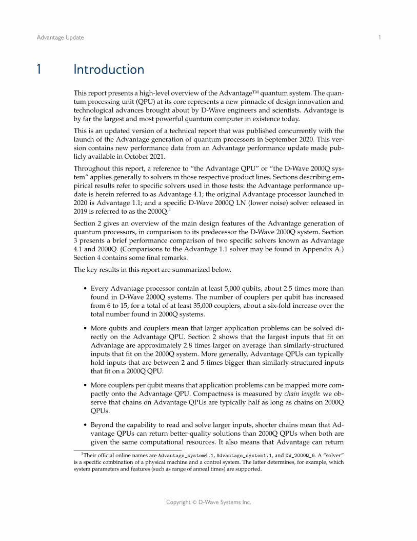
• Every Advantage processor contain at least 5,000 qubits, about 2.5 times more thanfound in D-Wave 2000Q systems. The number of couplers per qubit has increasedfrom 6 to 15, for a total of at least 35,000 couplers, about a six-fold increase over thetotal number found in 2000Q systems.

• More qubits and couplers mean that larger application problems can be solved di-rectly on the Advantage QPU. Section 2 shows that the largest inputs that fit onAdvantage are approximately 2.8 times larger on average than similarly-structuredinputs that fit on the 2000Q system. More generally, Advantage QPUs can typicallyhold inputs that are between 2 and 5 times bigger than similarly-structured inputsthat fit on a 2000Q QPU.

• More couplers per qubit means that application problems can be mapped more com-pactly onto the Advantage QPU. Compactness is measured by chain length: we ob-serve that chains on Advantage QPUs are typically half as long as chains on 2000QQPUs.

• Beyond the capability to read and solve larger inputs, shorter chains mean that Ad-vantage QPUs can return better-quality solutions than 2000Q QPUs when both aregiven the same computational resources. It also means that Advantage can return

1Their official online names are Advantage_system4.1, Advantage_system1.1, and DW_2000Q_6. A “solver”is a specific combination of a physical machine and a control system. The latter determines, for example, whichsystem parameters and features (such as range of anneal times) are supported.


Advantage Update 2

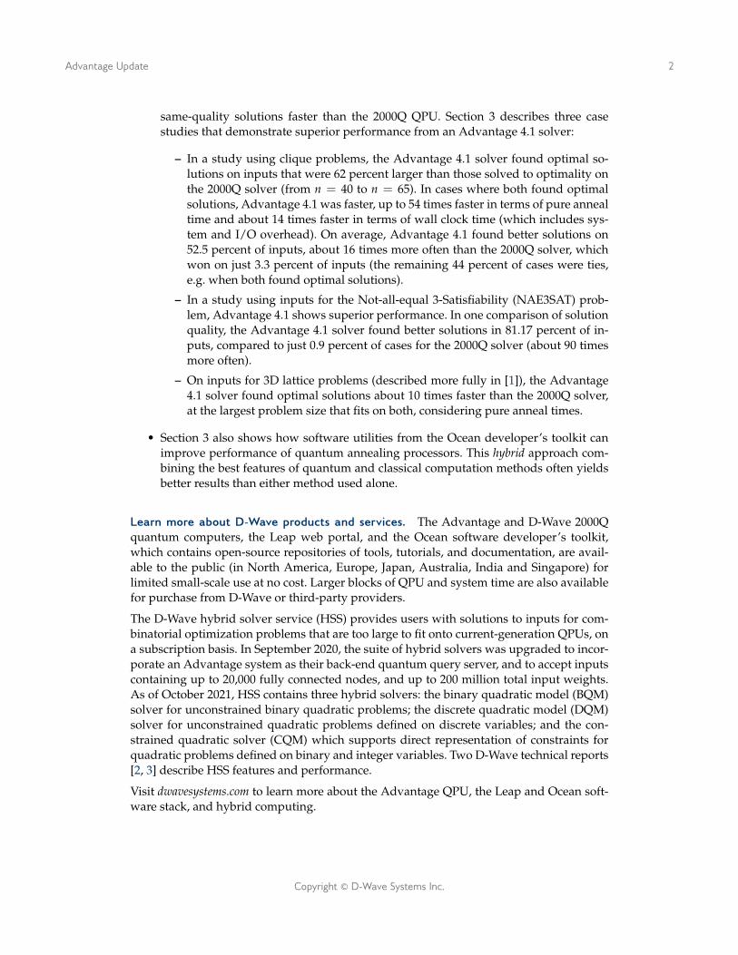
same-quality solutions faster than the 2000Q QPU. Section 3 describes three casestudies that demonstrate superior performance from an Advantage 4.1 solver:

– In a study using clique problems, the Advantage 4.1 solver found optimal so-lutions on inputs that were 62 percent larger than those solved to optimality onthe 2000Q solver (from n = 40 to n = 65). In cases where both found optimalsolutions, Advantage 4.1 was faster, up to 54 times faster in terms of pure annealtime and about 14 times faster in terms of wall clock time (which includes sys-tem and I/O overhead). On average, Advantage 4.1 found better solutions on52.5 percent of inputs, about 16 times more often than the 2000Q solver, whichwon on just 3.3 percent of inputs (the remaining 44 percent of cases were ties,e.g. when both found optimal solutions).

– In a study using inputs for the Not-all-equal 3-Satisfiability (NAE3SAT) prob-lem, Advantage 4.1 shows superior performance. In one comparison of solutionquality, the Advantage 4.1 solver found better solutions in 81.17 percent of in-puts, compared to just 0.9 percent of cases for the 2000Q solver (about 90 timesmore often).

– On inputs for 3D lattice problems (described more fully in [1]), the Advantage4.1 solver found optimal solutions about 10 times faster than the 2000Q solver,at the largest problem size that fits on both, considering pure anneal times.

• Section 3 also shows how software utilities from the Ocean developer’s toolkit canimprove performance of quantum annealing processors. This hybrid approach com-bining the best features of quantum and classical computation methods often yieldsbetter results than either method used alone.

Learn more about D-Wave products and services. The Advantage and D-Wave 2000Qquantum computers, the Leap web portal, and the Ocean software developer’s toolkit,which contains open-source repositories of tools, tutorials, and documentation, are avail-able to the public (in North America, Europe, Japan, Australia, India and Singapore) forlimited small-scale use at no cost. Larger blocks of QPU and system time are also availablefor purchase from D-Wave or third-party providers.

The D-Wave hybrid solver service (HSS) provides users with solutions to inputs for com-binatorial optimization problems that are too large to fit onto current-generation QPUs, ona subscription basis. In September 2020, the suite of hybrid solvers was upgraded to incor-porate an Advantage system as their back-end quantum query server, and to accept inputscontaining up to 20,000 fully connected nodes, and up to 200 million total input weights.As of October 2021, HSS contains three hybrid solvers: the binary quadratic model (BQM)solver for unconstrained binary quadratic problems; the discrete quadratic model (DQM)solver for unconstrained quadratic problems defined on discrete variables; and the con-strained quadratic solver (CQM) which supports direct representation of constraints forquadratic problems defined on binary and integer variables. Two D-Wave technical reports[2, 3] describe HSS features and performance.

Visit dwavesystems.com to learn more about the Advantage QPU, the Leap and Ocean soft-ware stack, and hybrid computing.


Advantage Update 3

Figure 1: A C6 Chimera graph (left) with 36 unit cells containing 288 qubits. A P4 Pegasus graph(right) with 27 unit cells and several partial cells, containing 264 qubits. The comparatively rich con-nectivity structure of the P4 is clearly seen.

2 New Advantage FeaturesIn a quantum annealing system, the hardware graph topology describes the pattern of physi-cal connections for qubits and the couplers between them. The most important and obviousdifference between D-Wave 2000Q and Advantage QPUs is the upgrade from Chimera tothe Pegasus topology, as shown in Figure 1.

The figure compares a C6 Chimera graph — a 6-by-6 grid of unit cells – with a P4 Pega-sus graph, which contains 27 unit cells on a diagonal grid, plus partial cells around theperimeter (note that unit cells on the Pegasus graph contain four extra couplers). Bothgraphs contain about the same number of qubits: the C6 has 288 and the P4 has 264. How-ever, Chimera has just 6 couplers per qubit while Pegasus has 15 couplers per qubit. Thiscreates the visibly more complex connection structure in Pegasus.

In addition to greater size and connectivity, the Pegasus graph has been modified in otherways to improve performance. For example, Pegasus contains triangles, which means thatmore general (nonbipartite) graph structures can be represented directly by the physicalhardware. See [4] for discussion of these and other properties.

Note that the physical hardware graphs inside the 2000Q and Advantage QPUs are muchlarger than shown in the figure: the former contains a C16 and the latter contains a P16.

Table 1 presents a comparison of the two QPU models in terms of typical componentcounts. The exact number of active qubits and couplers can vary across individual QPUs,because a small percentage of components may fail to meet technical specifications. Thetable shows the minimum number of active qubit and couplers in any QPU that is madeavailable to the public.

The following sections illustrate the connection between higher-degree connectivity struc-


Advantage Update 4

2000Q AdvantageGraph topology Chimera PegasusGraph size C16 P16Number of qubits > 2000 > 5000Number of couplers > 6000 > 35, 000Couplers per qubit 6 15

Table 1: Typical characteristics of Chimera- and Advantage-generation QPUs.

tures, which produce more compact embeddings with shorter chains, and QPU perfor-mance in terms of better solution quality and faster computation times.

Section 2.1 discusses general properties of the Advantage and D-Wave 2000Q processorgenerations. As mentioned in the introduction, Sections 2.2 and 2.3 present results of anempirical study performed on two specific solvers, here referred to as Advantage 4.1 and2000Q. Appendix A contains results of similar tests run on the original Advantage 1.1 sys-tem launched in September 2020.

2.1 More Compact Embeddings

An application input I for some problem P typically goes through two transformationsteps before being sent to a D-Wave QPU. The first step is to reformulate I as an input forthe quadratic unconstrained binary optimization problem (QUBO) (or for the equivalentIsing Model problem (IM)). This reformulation step uses standard cookbook techniquesfrom NP-completeness theory and is not further discussed here; see [5] for more.

The resulting QUBO input is represented by a so-called logical graph G containing n nodesand m edges; the input is specified by the pair (h, J) consisting of a set of n node weightsh = {hi} and m edge weights J = {Jij}. In order to be solved directly on a given QPU,the graph G must be mapped onto the physical hardware graph of qubits and couplers, e.g.Chimera or Pegasus.

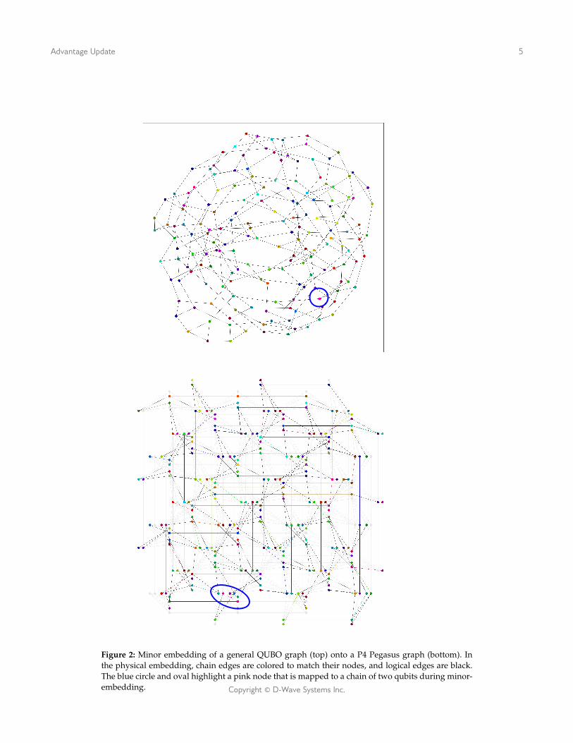
This mapping is normally performed by software utilities available in the Ocean develop-ers toolkit, using a technique called minor embedding (or informally, embedding). Figure 2shows an example graph G before and after minor-embedding onto a P4 Pegasus graph.The P4 embedding contains color-coded chains: each chain of qubits and couplers corre-sponds to a single node of the same color in the logical graph. For example, the blue ovalshighlight a pink node that is mapped to a chain of two qubits during minor-embedding.The logical edges of G are shown in black on the P4; qubits and couplers that are not usedin the embedding are shown in light grey.

The greater connectivity of Pegasus compared to Chimera means that the same logicalgraph can be minor-embedded more compactly onto the physical hardware. This fact hastwo important consequences:

• Minor embeddings on the Advantage QPU use fewer qubits per node, so the samenumber of qubits can hold larger logical graphs. This boosts the input capacity of theAdvantage QPU beyond that obtained by simply increasing the qubit count.

• Advantage embeddings generally require shorter chains than 2000Q embeddings.


Advantage Update 5

Figure 2: Minor embedding of a general QUBO graph (top) onto a P4 Pegasus graph (bottom). Inthe physical embedding, chain edges are colored to match their nodes, and logical edges are black.The blue circle and oval highlight a pink node that is mapped to a chain of two qubits during minor-embedding. Copyright © D-Wave Systems Inc.

Advantage Update 6

Shorter chains are stronger chains, which means the Advantage QPU can returnbetter-quality solutions than the 2000Q QPU.

These two points are illustrated and quantified in the following sections.

2.2 Bigger Inputs, Shorter Chains

The degree of a graph is the maximum number of edges per node. The logical graph ofFigure 2 has degree d = 3, which makes it fairly sparse and relatively easy to minor-embed into the Pegasus graph. In contrast, a fully-connected graph on n nodes, knownas a clique, has degree d = n − 1. Cliques are among the hardest graphs to embed onhardware topologies having limited connectivity, and tend to produce the longest chainsof any logical graph type.

The graph at the top of Figure 3 compares clique embeddings obtained using the Advan-tage 4.1 P16 topology (orange) and a 2000Q C16 (blue). Each curve shows the largest cliquesize that can be embedded using a given chain length. With chains of length 17, the P16 canhold cliques of size up to n = 177, while the C16 can only hold cliques of size up to n = 64.A graph of size n = 64 requires chains of length 17 on the C16 but only needs chains oflength 7 on the P16. That is, compared to the 2000Q QPU, the Advantage QPU can embedcliques that are almost three times as big, using chains that are less than half as long.

The middle table compares maximum embeddable graph sizes for some representativegraph types, ordered by increasing degree. The first two columns show the graph familyand the typical number of edges per node. For comparison to embedded inputs, the toprow shows maximum sizes for native inputs, which are identical to the physical hardwaregraph and require no chains.

Embedded three-dimensional lattices (described in Section 3.2) contain defects (missingnodes) due to imperfect qubit yield: the largest such lattice that can fit on a C16 is 8× 8× 8and the largest that its on a P16 is 15 × 15 × 12. Not-all-equal 3-Satisfiability problems(also described in Section 3.2) are random boolean expressions containing v variables andc triplet clauses, with a clause-to-variable ratio of ρ = 3; shown in the table are meandegrees for random inputs. Cliques are fully-connected graphs with degree equal to n− 1for problem size n. The bottom table compares typical chain lengths for these graphs, wheninput sizes are matched to fit on both hardware graphs.

These results are consistent with others not shown in the table: the maximum-size inputthat can be embedded onto an Advantage QPU is typically between 2 and 5 times biggerthan similarly-structured inputs embeddable on a 2000Q QPU, around 3 times larger onaverage. Embedded chains are on average less than half as long on the Advantage 4.1 QPUas on the 2000Q QPU.

The clique embeddings were obtained using the polynomial-time find_clique utility, whichfinds clique embeddings containing chains of uniform length. The 3D lattice embeddingsuse a custom embedder that also returns uniform chain lengths. Minor-embeddings forrandom NAE3SAT inputs were found using the minorminer heuristic (available in the OceanSDK), which finds embeddings with chains of uneven length. The tables show average de-gree and maximum chain lengths for NAE3SAT embeddings. See [6, 7] to learn more aboutD-Wave embedding tools.


Advantage Update 7

1 3 5 7 9 11 13 15 17Chain Length

0

25

50

75

100

125

150

175

Larg

est C

lique

Size

P16 maxP16 Advantage 4.1C16

Maximum Graph SizesLogical Graph Degree C16 P16 Ratio

n n P16/C16Native Chi=6, Peg=15 2030 5627 2.83D lattice (w/defects) 6 512 2687 5.2NAE3SAT ρ = 3 18 90 252 2.8Clique Chi=63,Peg=176 64 177 2.8

Chain Lengths at Matched Graph SizesLogical Graph Graph C16 Chain P16 Chain Ratio

Size Length Length P16/C163D lattice (defects) (all n) 4 2 0.50NAE3SAT ρ = 3 n = 80 33 11 0.33Clique n = 64 17 7 0.41

Figure 3: The graph at top shows the largest input size for each chain length, when cliques are minor-embedded onto 2000Q C16 (blue) and Advantage 4.1 P16 (orange) hardware graphs. The gray stepcurve at top shows results for a perfect defect-free P16 graph, which the Advantage4.1 QPU verynearly achieves. The dotted gray lines illustrate the differences in graph sizes for equal chain lengths(177 vs. 64 for chain length 17), and in chain lengths for equal graph sizes (7 vs. 17 for N = 64). TheAdvantage 4.1 QPU can hold cliques that are almost three times larger, using chains that are abouthalf as long as those embedded on the 2000Q QPU. The middle table shows maximum embeddablegraph sizes for a variety of other input types: mean of ratios in the table is 3.4. The bottom tableshows maximum chain lengths for these input graph types, matched by size.


Advantage Update 8

2.3 Chain Length and Chain Strength

A logical input graph G must be minor-embedded onto the hardware graph H before beingsent to the QPU. Minor-embedding maps logical nodes with high degree in G into chains oflower-degree qubits in H; chained qubits are connected by couplers assigned a weight Jchainknown as the chain strength, which is normally set to a large-magnitude negative value toensure that chained qubits all have the same value in the output.

A broken chain contains qubit values that disagree; a broken solution contains at least onebroken chain. Broken chains are problematic because the qubits disagree as to what valueshould be assigned to their corresponding logical node in the original problem. Brokensolutions can either be discarded from the output sample or repaired using one of thepostprocessing utilities available in Ocean, as described in Section 3.1.

As a general rule, embeddings with shorter chains are preferred over embeddings withlonger chains simply because short chains have fewer opportunities to break. But chainstrength is also important: suppose the logical input weights (h, J) all lie in a range [−x, x].The optimal choice of chain strength relative to x lies in a sweet spot between two hazards,as outlined below.

• If−Jchain (a positive value) is small compared to x, then the embedded input (h, J, Jchain)might contain spurious ‘optimal’ solutions that encode broken chains. Assumingqubit q is incident on c couplers, of which 2 are used as chains and the rest used aslogical weights, it would be necessary to set −Jchain > (c− 2)x so the chain is strongenough to overcome the torque created by logical weights (in a worst-case scenario).

• On the other hand, setting −Jchain much higher than x creates a danger of compress-ing the problem weights in [−x, x] (and therefore the gaps between distinct solutionenergies) beyond the precision limits of the quantum control system. Conceptually,every problem sent to the QPU is first scaled to an energy range [−1, 1] relative to itslargest-magnitude weight (i.e. Jchain).2 For example, let d = c− 2. If −Jchain = d · x,then problem weights are scaled to [−1/d, 1/d]: if d is too large, the QPU may havedifficulty distinguishing one weight from another, leading to a deterioration in solu-tion quality.

The higher connectivity of the Pegasus graph means that minor-embedded inputs can fitmore compactly onto the physical graph, with shorter chains. However, qubits are incidenton 15 couplers (excepting boundary qubits), so that the chain ratio, of logical couplers tochain couplers per qubit, is typically 13/2. In a Chimera graph the chain ratio is only 4/2,which greatly reduces the hazard of setting Jchain too high. The ultimate question is whetherbenefits of shorter chains are enough to overcome the hazards of higher connectivity andgreater torque.

Figure 4 shows the net effect of these opposing forces in a comparison of Advantage 4.1 and2000Q processors. The inputs are random cliques of size n = [30, 40, 50, 60], with hi = 0 andrandom edge weights Jij ∈ {±1}.The table at the top of the figure shows chain lengths and chain ratios for each QPU: em-beddings on Advantage 4.1 have about half the chain length, but almost three times the

2The example in the text is presented for simplicity: D-Wave QPUs offer an extended_J_range option thatscales to the energy range [−2, 1], effectively doubling the compressed scale of logical weights.


Advantage Update 9

Chain Length Chain RatioProblem size n: 30 40 50 60

2000Q C16 9 11 14 17 4/2Advantage 4.1 P16 4 5 6 7 13/2

Figure 4: The table (top) compares chain lengths and chain ratios for the D-Wave 2000Q and Advan-tage 4.1 QPUs in clique embeddings of various sizes n. The rightmost column shows proportions ofchain couplers to problem couplers per node on Chimera and Pegasus graphs. The graph (bottom)shows the percentage of intact samples returned by 2000Q (blue) and Advantage (orange), whendifferent chain strengths Jchain = [2, 4, 6, 8] are assigned.

chain ratio, as embeddings on 2000Q.

The graph below shows the effects of problem size and chain strength on the proportionP of unbroken solutions in sampled outputs from the Advantage 4.1 (orange) and 2000Q(blue) QPUs. For each n we generated 10 random inputs and embedded them with thefind_clique_embedding utility, using four different chain strengths Jchain = 6, 8, 10, 12.The anneal time was set to 200µs and the extended_j_range feature was enabled. Thevertical bars show the median values of P observed over all inputs, in samples of 1000outputs.

The graph shows that across a range of problem sizes and chain strengths, the upgradeto Pegasus is beneficial: Advantage 4.1 returns values of P that are competitive with andsometimes better than, those returned by 2000Q processor. (Note that relative performancein P for very low chain strength 6 is likely due to the introduction of spurious optimalsolutions as described above: Advantage 4.1 returns more broken solutions because theyare optimal but spurious, created by setting chain strength too low.)

The next section shows how this ability to support stronger chains with smaller chainstrengths translates into better-quality solutions from the Advantage QPU.

3 Performance ComparisonThis section considers performance of the Advantage 4.1 and the 2000Q solvers, in termsof the quality of solutions they find. Results of similar tests on the Advantage 1.1 solvermay be found in Appendix A.


Advantage Update 10

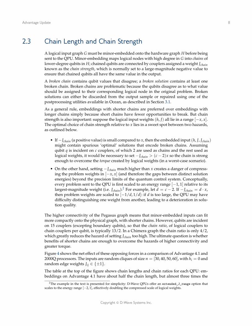
Figure 5: The graphs compare solution quality found by the 2000Q (blue) and Advantage 4.1 (or-ange) QPUs when chain strengths are set to Jchain = 8 (too low for largest n). In the left panel, brokensolutions are discarded; in the right panel, broken solutions are repaired using Majority Vote post-processing. The points show the lowest relative error L, for ten trials at each n, and the lines connectdata medians. A value of L = 0 indicates the reference solution was found in the solution sample;a value of L > 0 shows the scaled distance to this putative ground state. Missing points and linesindicate L = NA: either the sample contains no intact solutions (left panel), or the problem is too bigto fit on the QPU (right panel). For each QPU, a pair of vertical dotted lines indicates the transitionpoints from L = 0 to L > 0, and from L > 0 to L = NA.

Rather than evaluate raw hardware performance, we take a user-centric and system-centricapproach by making use of tools and utilities available in the Ocean SDK, as described inSection 3.1. Section 3.2 evaluates performance of the Advantage and 2000Q quantum sys-tems on the clique problems from Section 2, as well as two additional problem categoriesknown as NAE3SAT and 3DLattice.

3.1 Hardware and Software Better Together

The open-source Ocean SDK [8, 9] is part of a broad effort by D-Wave developers andengineers to make quantum-based problem-solving accessible to the computing public, byleveling out the learning curve associated with quantum computation. Growing experiencewith Ocean tools suggests that hybrid methods combining the best features of quantumand classical computation can often produce better results than either approach used alone.

For example, a fast and simple postprocessing utility known as majority voting (MV) canboost the quality of raw QPU results by repairing broken chains in output solutions. Thisutility, which is invoked by default in some QPU-based Ocean solvers, assigns a value toeach logical node based on a “vote” of the qubits in its corresponding chain (breaking tiesat random). Thus, the MV postprocessor converts all broken solutions into intact solutions,in just a few microseconds per output. (Ocean provides other chain-repair strategies notdiscussed here; see [10] for details.)

Chain repair is especially valuable in use cases that require quick response from the quan-tum system, in which case exploratory work to find optimal chain strengths is not an op-tion. To demonstrate this point, we generate ten random clique inputs at each problem size


Advantage Update 11

n = [5, 10, . . . , 120], and additionally at the largest sizes embeddable on each QPU, n = 64and n = 177. We set Jchain = 8 for all n, which is too low for the largest problem sizes (seeFigure 6), producing a too-high proportion of broken chains.

For each input we request a sample of 1000 solutions, using anneal time 200µs, with theextended_j_range option turned on. We measure solution quality with respect to a refer-ence energy Ere f , corresponding to a putative optimal solution for each input. That is, sinceit is computationally infeasible to compute certifiably optimal solutions at the largest prob-lem sizes tested, we instead employ a reliable classical heuristic running for a long time tofind putative optimal solutions.

The solution quality metric is lowest relative error, denoted L. For each input we take 1000solution samples from the QPU and either discard (left panel) or repair (right panel) thebroken solutions. The lowest relative error is the scaled difference between the referenceenergy and the lowest energy found in the resulting sample:

L =∆(Ere f , Elow)

|Ere f |,

Where ∆(Ere f , Elow) is the positive distance between the two energies, accounting for pos-sible sign differences. This metric can be interpreted as follows:

• At small n we observe L = 0, indicating that the QPU can find at least one referencesolution in the sample. With 1000 solutions this corresponds to achieving a thresholdsuccess probability of π > 0.001.

• At larger n we observe L > 0, in which case L shows the scaled distance between thesample minimum and the reference solution.

• At even larger n we observe L = NA, that is, the statistic could not be computedbecause no viable results were returned. This happens for one of two reasons: (1) theQPU returns no solutions because the input is too large to fit; or (2) the solution sam-ple from the QPU contained no intact (unbroken) solutions and all were discarded.

Figure 5 shows the results of setting the chain strength parameter too low, with and with-out MV postprocessing. The left panel shows solution quality when broken solutions arediscarded from the sample, and the right panel shows solution quality when MV postpro-cessing is used to repair all broken solutions.

In both panels, the points show values of L returned by the 2000Q (blue) and Advantage4.1 (orange) QPUs for each input, and the lines connect medians over n. For each QPUa pair of horizontal bars above the data points show regions bounded by two transitionpoints in n: from L = 0 to L > 0 (left bar endpoint) and from L > 0 to L = NA (right barendpoint). Here are some observations.

• Comparing left endpoints, we see that Advantage 4.1 can find optimal solutions atlarger problem sizes than the 2000Q QPU: the transition point is 62% higher (fromn = 40 to n = 65) when considering raw QPU outputs and 60% higher (n = 50 ton = 80) after postprocessing.

• Comparison of right endpoints shows that Advantage 4.1 finds intact solutions athigher n. On the left panel, Advantage 4.1 goes 40% higher n than the 2000Q QPU


Advantage Update 12

(n = 50 vs. n = 70). On the right panel, we see that Advantage 4.1 is able to realizethe full potential of higher qubit counts and greater connectivity, finding solutionsto problems of size up to n = 177, 2.8 times as big as n = 64 for the 2000Q QPU.The highest relative error from the 2000Q QPU is around 0.05 at n = 65: note thatAdvantage 4.1 achieves the same-quality performance on problems that are 2.5 timeslarger, at n = 125.

• In both panels, the region marked by orange bars is strictly to the right of the regionmarked by blue bars: in this test the Advantage 4.1 QPU can find optimal solutionsat problem sizes for which the 2000Q solver fails to find any viable solutions at all.

MV postprocessing improves performance of both QPUs in this case and in general; forthis reason the performance tests in the next section incorporate this Ocean feature.

3.2 Performance Analysis

Better embeddings on the Pegasus topology, plus better raw performance due to new ma-terials and design processes, means that the Advantage 4.1 QPU can return better-qualitysolutions than the 2000Q QPU on some inputs. It also means that Advantage 4.1 can findsame-quality solutions faster (needing fewer samples), and that Advantage 4.1 can solveproblems to optimality at higher input sizes n.

This section describes three small case studies using embedded inputs to compare per-formance of the two QPUs under a various performance metrics. In all three cases theAdvantage 4.1 QPU achieves equal or superior performance to the 2000Q QPU.

Random Cliques In this section we compare performance of an Advantage 4.1 and 2000Qsystem using the clique inputs described in the previous section. We generate 10 randomcliques at each problem size n = [10, . . . , 60]. Anneal time is set to 200µs, R = 1000 outputsamples are read, and the extended_j_range option is turned on. The MV postprocessingtool was used throughout these tests.

A small exploratory study was performed to identify optimal values for chain strengthJchain, for each QPU and each input size n. The study considered integer values of Jchain aswell as a functional form Jchain = c

√n found by a regression analysis on each QPU.

Here, Jchain was selected to minimize the median relative error metric M, similar to the lowestrelative error L from the previous section, except computed on the sample median insteadof the sample minimum. Although L is arguably more interesting to practitioners, we useM instead because both QPUs frequently find optimal solutions on these problems, withthe result that L = 0 in nearly all cases; for this reason L cannot be used to optimize param-eters, nor to distinguish performance of the two quantum processors.

The results are shown in Figure 6. The table at top shows the best chain strength Jchainfound in the exploratory study. The one case of non-monotonicity in the table appears tobe due to experimental noise: we note that both quantum processors can tolerate someimprecision in selection of optimal Jchain, since values within, say,±2 of those shown in thetable have nearly imperceptible effect on solution quality as measured by M.


Advantage Update 13

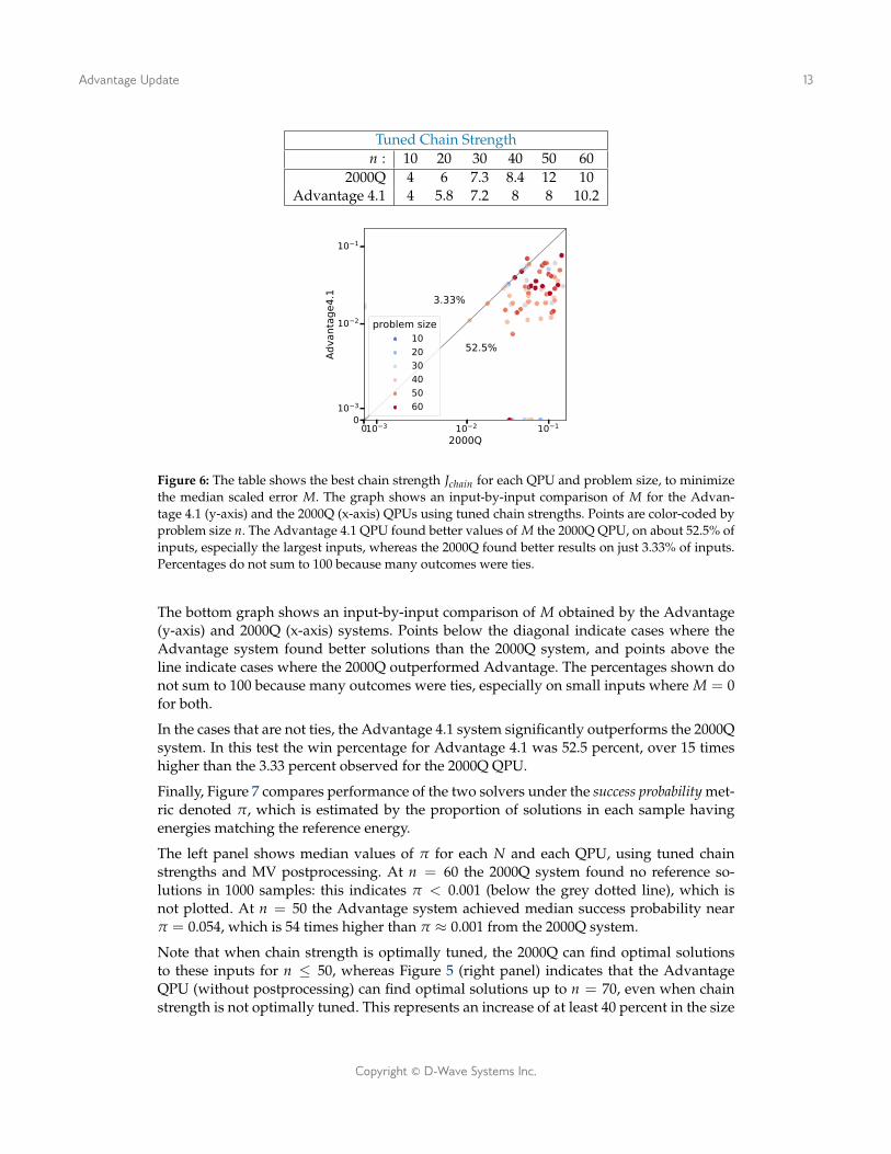
Tuned Chain Strengthn : 10 20 30 40 50 60

2000Q 4 6 7.3 8.4 12 10Advantage 4.1 4 5.8 7.2 8 8 10.2

010 3 10 2 10 1

2000Q0

10 3

10 2

10 1

Adva

ntag

e4.1

52.5%

3.33%

problem size102030405060

Figure 6: The table shows the best chain strength Jchain for each QPU and problem size, to minimizethe median scaled error M. The graph shows an input-by-input comparison of M for the Advan-tage 4.1 (y-axis) and the 2000Q (x-axis) QPUs using tuned chain strengths. Points are color-coded byproblem size n. The Advantage 4.1 QPU found better values of M the 2000Q QPU, on about 52.5% ofinputs, especially the largest inputs, whereas the 2000Q found better results on just 3.33% of inputs.Percentages do not sum to 100 because many outcomes were ties.

The bottom graph shows an input-by-input comparison of M obtained by the Advantage(y-axis) and 2000Q (x-axis) systems. Points below the diagonal indicate cases where theAdvantage system found better solutions than the 2000Q system, and points above theline indicate cases where the 2000Q outperformed Advantage. The percentages shown donot sum to 100 because many outcomes were ties, especially on small inputs where M = 0for both.

In the cases that are not ties, the Advantage 4.1 system significantly outperforms the 2000Qsystem. In this test the win percentage for Advantage 4.1 was 52.5 percent, over 15 timeshigher than the 3.33 percent observed for the 2000Q QPU.

Finally, Figure 7 compares performance of the two solvers under the success probability met-ric denoted π, which is estimated by the proportion of solutions in each sample havingenergies matching the reference energy.

The left panel shows median values of π for each N and each QPU, using tuned chainstrengths and MV postprocessing. At n = 60 the 2000Q system found no reference so-lutions in 1000 samples: this indicates π < 0.001 (below the grey dotted line), which isnot plotted. At n = 50 the Advantage system achieved median success probability nearπ = 0.054, which is 54 times higher than π ≈ 0.001 from the 2000Q system.

Note that when chain strength is optimally tuned, the 2000Q can find optimal solutionsto these inputs for n ≤ 50, whereas Figure 5 (right panel) indicates that the AdvantageQPU (without postprocessing) can find optimal solutions up to n = 70, even when chainstrength is not optimally tuned. This represents an increase of at least 40 percent in the size


Advantage Update 14

Figure 7: The graph shows median success probabilities for Advantage4.1 and 2000Q QPUs on ran-dom cliques. In these tests using 1000 reads, a success probability below 0.001 (i.e. below the graydotted line), as observed for 2000Q at n = 60, is recorded as zero and not shown on this logarithmicscale. Throughout this range of problem sizes, the Advantage 4.1 QPU achieves higher success prob-abilities than the 2000Q QPU. The right panel shows 1/π, corresponding to the expected sample sizeneeded to observe a reference solution in the output sample. At n = 50, the expected sample size isabout 54 times smaller for Advantage 4.1 than for the 2000Q QPU.

of inputs that can be solved to optimality.

The right panel shows R = 1/π, corresponding to the expected number of solution sam-ples needed to observe a reference solution. Expected sample size R corresponds roughlyto the computation time needed to find reference solutions, although times at small valuesof R such as these tend to be dominated by chip I/O overhead. In this context, a 54-foldspeedup in R maps to over a 14-fold speedup in wall clock time, from about 0.42 secondsto 0.03 seconds.

NAE3SAT Inputs Next we compare QPU performance on inputs for the Not-All-Equal 3-Satisfiability (NAE3SAT) problem. A random NAE3SAT input is a boolean expression withn variables v = {v1, . . . vn} organized in m clauses: each clause contains three randomly-selected variables or their negations. A clause is satisfied (i.e., has the value True) if thevalues of the three elements are not all equal. Clauses are joined by disjunctions (logical”and”), so that the whole formula is satisfied only when every clause is True.

The combinatorial hardness of random formulas constructed this way depends on theclause-to-variable ratio ρ = m/n. Our tests use random NAE3SAT inputs generated atρ = 2.1 (interesting for testing performance at finding optimal solutions) and at ρ = 3 (in-teresting for testing performance at finding approximate solutions). The boolean expres-sions thusly generated are translated into QUBO logical inputs using standard techniques.The logical graphs resulting from problems generated at ρ = 2.1 and ρ = 3 have averagenode degrees 13.2 and 18, respectively.

These inputs were embedded using the heuristic find_embedding tool available in Ocean.


Advantage Update 15

ρ = 2.1 ρ = 3

0 10 2 10 1

2000Q0

10 2

10 1

Adva

ntag

e4.1

81.17%

0.9%


0 10 2 10 1

2000Q0

10 2

10 1

Adva

ntag

e4.1

78.65%

1.56%

problem size104070

Figure 8: The left and right panels show results for ρ = 2.1 and ρ = 3, respectively. Maximum inputsize is n = 100 in the left panel and n = 90 in the right panel. The graphs present input-by-inputcomparisons of median relative error M, for the Advantage 4.1 (y-axis) and 2000Q (x-axis) QPUs.In each panel, points below the diagonal line indicate cases where Advantage 4.1 returned superiorsolutions. The percentages do not sum to 100 because many ties were observed.

This embedder differs from the polynomial-time find_clique_embedding tool used forclique inputs in several ways, for example: embeddings may contain chains of varyinglength, and different runs will produce different embeddings. See [6, 7] for more aboutembedders in Ocean.

In these tests we generated five random inputs at each problem size n ∈ [10, 12, . . . , nρ]where n2.1 = 100 and h3 = 90. For these types of inputs, the minimum and maximumchain lengths in a given embedding tend to differ by a factor of about two. Embeddings onthe Advantage 4.1 QPU tend to have mean and maximum chain lengths about half as longas embeddings on the 2000Q QPU.

Putative optimal solution energies were obtained using reliable heuristics applied to thelogical problems. For each input we took 1000 samples from each QPU. Anneal time wasset to 200µs; chain strength was set to Jchain = −3 (based on an exploratory study); and theMV postprocessing option was selected.

The results appear in the two graphs of Figure 8, which show input-by-input comparisonsof Advantage (orange) and 2000Q (blue) performance, for input sets ρ = 2.1 (left panel)and ρ = 3 (right panel).

Solution quality is measured by the median relative error metric M described in the previ-ous section. Points below the diagonal line correspond to cases where the Advantage QPUreturned strictly better solutions than the 2000Q QPU. The win percentages shown in thepanels do not sum to 100 because the two QPUs tied in many cases.

As before, the Advantage system finds better solutions than the 2000Q systems on a higherproportion of inputs. For ρ = 2.1 the 81.17% win percentage is about 90 times higher, andfor ρ = 3 the 78.65% percentage is about 50 times higher.


Advantage Update 16

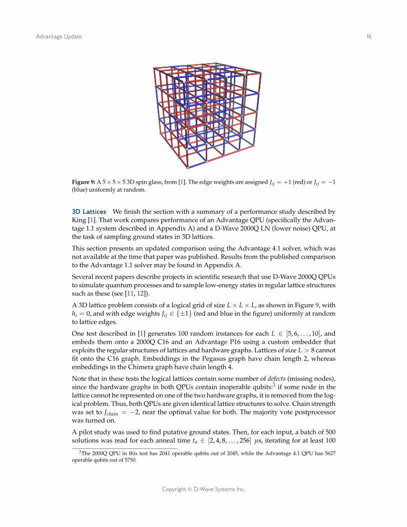
Figure 9: A 5× 5× 5 3D spin glass, from [1]. The edge weights are assigned Jij = +1 (red) or Jij = −1(blue) uniformly at random.

3D Lattices We finish the section with a summary of a performance study described byKing [1]. That work compares performance of an Advantage QPU (specifically the Advan-tage 1.1 system described in Appendix A) and a D-Wave 2000Q LN (lower noise) QPU, atthe task of sampling ground states in 3D lattices.

This section presents an updated comparison using the Advantage 4.1 solver, which wasnot available at the time that paper was published. Results from the published comparisonto the Advantage 1.1 solver may be found in Appendix A.

Several recent papers describe projects in scientific research that use D-Wave 2000Q QPUsto simulate quantum processes and to sample low-energy states in regular lattice structuressuch as these (see [11, 12]).

A 3D lattice problem consists of a logical grid of size L× L× L, as shown in Figure 9, withhi = 0, and with edge weights Jij ∈ {±1} (red and blue in the figure) uniformly at randomto lattice edges.

One test described in [1] generates 100 random instances for each L ∈ [5, 6, . . . , 10], andembeds them onto a 2000Q C16 and an Advantage P16 using a custom embedder thatexploits the regular structures of lattices and hardware graphs. Lattices of size L > 8 cannotfit onto the C16 graph. Embeddings in the Pegasus graph have chain length 2, whereasembeddings in the Chimera graph have chain length 4.

Note that in these tests the logical lattices contain some number of defects (missing nodes),since the hardware graphs in both QPUs contain inoperable qubits:3 if some node in thelattice cannot be represented on one of the two hardware graphs, it is removed from the log-ical problem. Thus, both QPUs are given identical lattice structures to solve. Chain strengthwas set to Jchain = −2, near the optimal value for both. The majority vote postprocessorwas turned on.

A pilot study was used to find putative ground states. Then, for each input, a batch of 500solutions was read for each anneal time ta ∈ [2, 4, 8, . . . , 256] µs, iterating for at least 100

3The 2000Q QPU in this test has 2041 operable qubits out of 2045, while the Advantage 4.1 QPU has 5627operable qubits out of 5750.


Advantage Update 17

103 104 105 106 107 108

103

104

105

106

107

108

DW2000Q LN TTS (µs)

AdvantageTTS(µs)

8×8×8 instances

log-log �t line

6 8 10101

102

103

104

105

106

107

108

Lattice dimension L

Timeto

solution(µs)

DW2000Q LN

Advantage

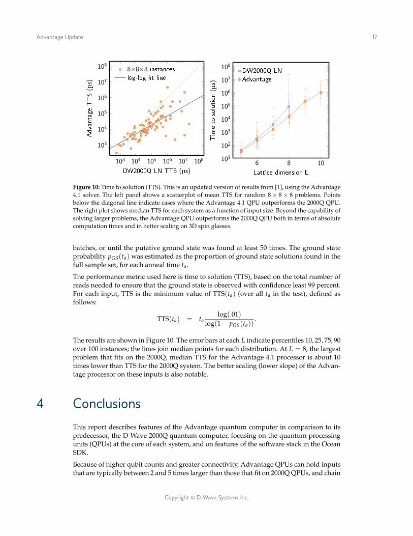
Figure 10: Time to solution (TTS). This is an updated version of results from [1], using the Advantage4.1 solver. The left panel shows a scatterplot of mean TTS for random 8 × 8 × 8 problems. Pointsbelow the diagonal line indicate cases where the Advantage 4.1 QPU outperforms the 2000Q QPU.The right plot shows median TTS for each system as a function of input size. Beyond the capability ofsolving larger problems, the Advantage QPU outperforms the 2000Q QPU both in terms of absolutecomputation times and in better scaling on 3D spin glasses.

batches, or until the putative ground state was found at least 50 times. The ground stateprobability pGS(ta) was estimated as the proportion of ground state solutions found in thefull sample set, for each anneal time ta.

The performance metric used here is time to solution (TTS), based on the total number ofreads needed to ensure that the ground state is observed with confidence least 99 percent.For each input, TTS is the minimum value of TTS(ta) (over all ta in the test), defined asfollows:

TTS(ta) = talog(.01)

log(1− pGS(ta)).

The results are shown in Figure 10. The error bars at each L indicate percentiles 10, 25, 75, 90over 100 instances; the lines join median points for each distribution. At L = 8, the largestproblem that fits on the 2000Q, median TTS for the Advantage 4.1 processor is about 10times lower than TTS for the 2000Q system. The better scaling (lower slope) of the Advan-tage processor on these inputs is also notable.

4 ConclusionsThis report describes features of the Advantage quantum computer in comparison to itspredecessor, the D-Wave 2000Q quantum computer, focusing on the quantum processingunits (QPUs) at the core of each system, and on features of the software stack in the OceanSDK.

Because of higher qubit counts and greater connectivity, Advantage QPUs can hold inputsthat are typically between 2 and 5 times larger than those that fit on 2000Q QPUs, and chain


Advantage Update 18

lengths are generally half as long.

The performance comparison in Section 3.2 compares a specific Advantage system (re-ferred to here as Advantage 4.1) to a specific 2000Q LN system (referred to as 2000Q),using three categories of embedded inputs: cliques, NAE3SAT inputs, and 3D lattices.

Results from this section demonstrates that, beyond the ability to solve larger problems, theAdvantage 4.1 solver can find better-quality solutions than the 2000Q solver when both areallowed equivalent computational resources (cliques and NAE3SAT problems); Advantage4.1 can also find equivalent-quality solutions faster, and can solve problems to optimalityat larger problem sizes (cliques and 3D lattices).

We attribute this performance improvement to the new Pegasus graph topology and itssupport for shorter and stronger chains in minor-embedded inputs. Furthermore, the Ad-vantage 4.1 solver incorporates several technological innovations — in chip design, ma-terials, and fabrication processes — to achieve better overall performance than the firstAdvantage 1.1 solver.

The tests described in this report focus on performance as would be experienced by prac-titioners with real-world applications, by considering logical input classes that must beembedded onto the respective QPUs. Furthermore, our tests consider the performance ofthe QPUs when used in combination with tools found in the Ocean SDK.

The preliminary results presented here are only the beginning: we look forward to moreextensive performance studies and to more demonstrations of superior performance incomparison to both quantum and classical alternatives, for Advantage quantum systems,as well as to future generations of D-Wave annealing-based quantum computes.

References1 A. King and W. Bernoudy, “Performance benefits of increased qubit connectivity in quantum annealing 3-dimensional spin glasses,”

arXiv:200912479[quant-ph] (2020).

2 C. McGeoch et al., Hybrid Solver Service + Advantage: Technology Update, dwavesys.com/resources (2020).

3 C. McGeoch and P. Farré, Hybrid Solver for Constrained Quadratic Models, dwavesys.com/resources (2021).

4 K. Boothby et al., Next-Generation Topology of D-Wave Quantum Processors, dwavesys.com/resources (2019).

5 A. Lucas, “Ising formulations of many NP problems,” Frontiers in Physics 2 (2014).

6 “D-Wave Ocean Software Documentation, keyword: minor embedding,” http://docs.ocean.dwavesys.com/en/stable/index.html(2020).

7 “D-Wave Ocean Software Documentation, keyword: find clique embedding,” http://docs.ocean.dwavesys.com/en/stable/index.html (2020).

8 “D-Wave’s Ocean Software,” http://ocean.dwavesys.com (2020).

9 “D-Wave Ocean Software Documentation,” http://docs.ocean.dwavesys.com/en/stable/index.html (2020).

10 “D-Wave Ocean Software Docuentation, keyword: post processing,” http://docs.ocean.dwavesys.com/en/stable/index.html(2020).

11 R Harris, “Phase transitions in a programmable quantum spin glass simulator,” Science 316, 162–165 (2018).

12 A. King et al., “Observation of topological phenomenon in a programmable lattice of 1,800 qubits,” Nature 560, 456–460 (2018).

13 McGeoch, C. and Farré, P., The Advantage System: An Overview, dwavesys.com/resources (2020).


dwavesys.com/resources



http://docs.ocean.dwavesys.com/en/stable/index.html



http://ocean.dwavesys.com




Advantage Update 19

Appendix A: The Advantage 1.1 SolverThe launch of the first Advantage-generation processor in September 2020 (here referredto as Advantage 1.1) was accompanied by publication of a D-Wave Technical Report (TR)[13], comparing its performance to a previous-generation D-Wave 2000Q LN (lower noise)QPU.

The main text of this TR updates the performance analysis from that previous TR, witha comparison of the same 2000Q solver to an Advantage performance update (called theAdvantage 4.1 solver) that was made publicly available in October 2021.

This appendix preserves the data from the original TR, which describes results from iden-tical tests carried out on Advantage 1.1 and the 2000Q solver. These results, together withsome new direct comparisons of Advantage 1.1 and Advantage 4.1 QPUs, are presented inSection A.2.

In addition, Section A.1 describes a small study that compares performance of the Advan-tage 4.1 and Advantage 1.1 solvers using native (unembedded) inputs. This study high-lights performance upgrades within the same generation of Advantage quantum systems.

Overall, the Advantage 4.1 solver outperforms both the 2000Q solver and the Advantage1.1 solver in nearly every performance metric used in our tests.

Superior performance of Advantage-generation systems compared to 2000Q systems islargely due to the introduction of the Pegasus architecture, which has several beneficial fea-tures compared to the Chimera architecture used in D-Wave 2000Q and earlier-generationquantum systems.

Performance improvements within the same-generation Advantage product line may beattributed to technological advances that make possible higher qubit and coupler yields,as well as to innovations in chip design, and improvements in fabrication materials andprocesses.

A.1 Performance on Native Inputs

A native input for a quantum annealer is mapped directly onto qubits and couplers, andcontains no chains. Although native inputs are not tied to real-world applications, they giveinsight about raw performance of qubits and couplers inside a given quantum processor.

In this study we compare Advantage 4.1 (available in October 2021) to its predecessor Ad-vantage 1.1 (launched in September 2020). For accurate comparison, we use the intersectiongraph H∗ containing only qubits and couplers that are active on both processors.

For each problem size, we generate 101 RAN1 inputs on H∗, which have hi = 0, andJij = ±1 assigned uniformly at random. Problem sizes correspond to square subregions ofthe Pegasus graph, from P2 up to P16.

QPU parameters are set to anneal time tanneal = 200µs, and number of reads R = 1000 perinstance, with 10 spin reversal transforms per read.

For each instance we record the best energy B found among all solutions from both QPUs.For each solution S we compute the positive energy difference ∆(B, S) (accounting for pos-


Advantage Update 20

39 124

255

431

657

928

1245

1607

2018

2474

2967

3511

4098

4738

5423

Problem Size

010 4

10 3

10 2

10 1

(Sam

ple

Med

ian)

Rela

tive

Erro

r

Advantage1.1Advantage4.1

39 124

255

431

657

928

1245

1607

2018

2474

2967

3511

4098

4738

5423

Problem Size

0

10 4

10 3

10 2

10 1

(Sam

ple

Min

)Re

lativ

e Er

ror

Advantage1.1Advantage4.1

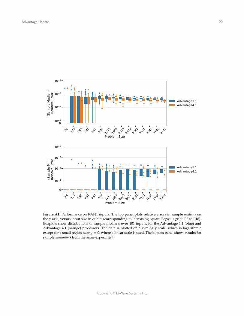
Figure A1: Performance on RAN1 inputs. The top panel plots relative errors in sample medians onthe y axis, versus input size in qubits (corresponding to increasing square Pegasus grids P2 to P16).Boxplots show distributions of sample medians over 101 inputs, for the Advantage 1.1 (blue) andAdvantage 4.1 (orange) processors. The data is plotted on a symlog y scale, which is logarithmicexcept for a small region near y = 0, where a linear scale is used. The bottom panel shows results forsample minimums from the same experiment.


Advantage Update 21

sible sign differences), and the relative error ρ = ∆(B, S)/|B|. A minimum relative errorρ = 0 is the best possible outcome in this metric.

Figure A1 shows the results of this experiment. The top panel shows a boxplot of the dis-tribution of relative errors from the median of each sample of size R returned by each pro-cessor. On smallest inputs, processor performance is nearly equivalent; on largest inputsthe distribution of median relative errors is consistently better for Advantage 4.1.

The bottom panel shows the distribution of relative errors from sample minimums in eachtest. At all input sizes, the bulk of the data distribution for Advantage 4.1 — covered byboxplot and tails — is located entirely at zero. This indicates that except for a few out-liers (orange diamonds), this the Advantage 4.1 solver found best sample minimums innearly every test on nearly every input. Advantage 1.1 achieves similar solution qualitiesat smallest input sizes, but the center and quartiles of the distribution of relative errorssteadily increase as input sizes grow above q = 657.

A.2 Tests from Sections 2 and 3

The figures appearing in this section may be compared to the same-numbered figures inSections 2 and 3 of the main text. See those sections for detailed descriptions of each testand its outcomes. Most graphs in this Appendix are taken from an earlier technical reportcomparing Advantage1.1 to the 2000Q QPU. A few additional graphics have been includedto facilitate direct comparison of all three solvers: Advantage 4.1, Advantage 1.1, and the2000Q.


Advantage Update 22

1 3 5 7 9 11 13 15 17Chain Length

0

25

50

75

100

125

150

175

Larg

est C

lique

Size

P16 maxP16 Advantage 4.1P16 Advantage 1.1C16

Maximum Graph SizesLogical Graph Degree C16 P16 Ratio

n n P16/C16Native Chi=6, Peg=15 2030 5436 2.73D lattice (w/defects) 6 512 2354 4.6NAE3SAT r = 2.1 13.2 100 286 2.9NAE3SAT r = 3 18 90 242 2.7Clique Chi=63, Peg=123 64 119 1.9

Chain Lengths at Matched Graph SizesLogical Graph Graph C16 Chain P16 Chain Ratio

Size Length Length P16/C163D lattice (defects) (all n) 4 2 .50NAE3SAT r = 2.1 n = 70 12 5 .42NAE3SAT r = 3.0 n = 70 15 7 .47Clique n = 60 16 7 .44

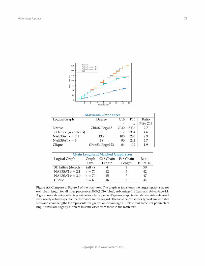
Figure A3: Compare to Figure 3 of the main text. The graph at top shows the largest graph size foreach chain length for all three processors: 2000Q C16 (blue), Advantage 1.1 (teal) and Advantage 4.1.A gray curve showing what is possible for a fully yielded Pegasus graph is also shown: Advantage 4.1very nearly achieves perfect performance in this regard. The table below shows typical embeddablesizes and chain lengths for representative graphs on Advantage 1.1. Note that some test parameters(input sizes) are slightly different in some cases from those in the main text.


Advantage Update 23

Chain Length per Problem SizeProblem size n: 30 40 50 60

2000Q C16 9 11 14 17Advantage 1.1 P16 4 6 7 9Advantage 4.1 P16 4 5 6 7

Figure A4: Compare to Figure 4 in the main text. The table (top) compares chain lengths for the2000Q, Advantage 1.1 and Advantage 4.1 solvers, in clique embeddings of various sizes n. The graph(bottom) shows the percentage of intact samples returned by the 2000Q (blue) and the Advantage 1.1(orange), when different chain strengths Jchain = [2, 4, 6, 8] are assigned. Interestingly, the fraction ofunbroken samples is slightly lower for Advantage 4.1 than for Advantage 1.1, even though solutionquality is uniformly better. This phenomenon will be examined further in a followup study.

Figure A5: Compare to Figure 5 in the main text. The graphs compare solution quality found by the2000Q (blue) and Advantage 1.1 (orange) QPUs when chain strengths are set to Jchain = 8, too lowfor large n. In the left panel, broken solutions are discarded; in the right panel, broken solutions arerepaired using majority vote postprocessing.


Advantage Update 24

Tuned Chain Strengthn : 10 20 30 40 50 60

2000Q 4 6 7.3 8.4 12 10Advantage 1.1 4 6 6 8 8 10Advantage 4.1 4 5.8 7.2 8 8 10.2

010 3 10 2 10 1

2000Q0

10 3

10 2

10 1Ad

vant

age

45.83%

6.67%


Figure A6: Compare to Figure 6 in the main text. The table shows the best chain strength Jchain foreach QPU by problem size, to minimize the median scaled error M. The left panel shows an input-by-input comparison of M for the Advantage 1.1 (y-axis) and the 2000Q (x-axis) QPUs using tuned chainstrengths. The right panel shows a comparison of the Advantage 4.1 (y-axis) and the Advantage 1.1(x-axis) QPUs. Percentages do not sum to 100 because many outcomes were ties.

Figure A7: Compare to Figure 7 in the main text. The left panel shows median success probabilities π

for Advantage 1.1 and 2000Q QPUs on random cliques; the right panel shows 1/π, corresponding tothe expected number of reads needed to observe an optimal solution. In these tests using 1000 reads,a success probability below 0.001 (i.e. below the gray dotted line), as observed for 2000Q at n = 60,is recorded as zero and not shown on this logarithmic scale.


Advantage Update 25

ρ = 2.1 ρ = 3

0 10 2 10 1

2000Q0

10 2

10 1

Adva

ntag

e

64.5%

3.9%


0 10 2 10 1

2000Q0

10 2

10 1

Adva

ntag

e

51.56%

16.67%

problem size104070

0 10 2 10 1

Advantage1.10

10 2

10 1

Adva

ntag

e4.1

57.39%

3.04%


0 10 2 10 1

Advantage1.10

10 2

10 1

Adva

ntag

e4.1

70.0%

3.04%


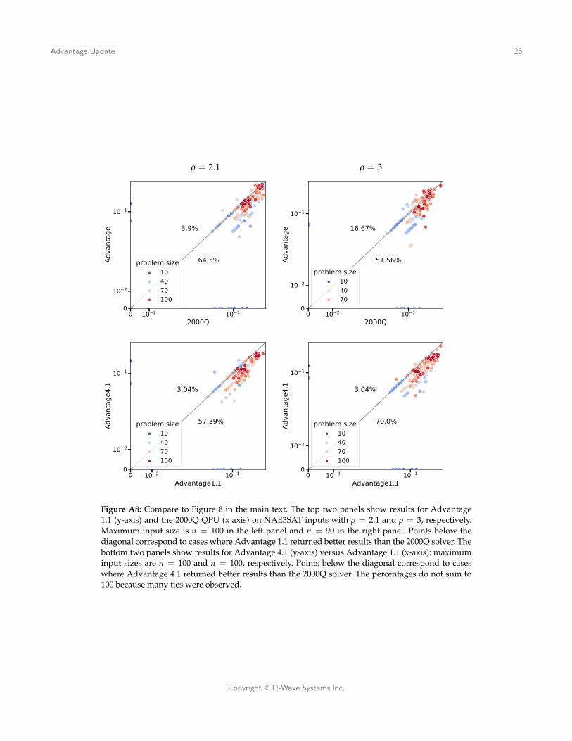
Figure A8: Compare to Figure 8 in the main text. The top two panels show results for Advantage1.1 (y-axis) and the 2000Q QPU (x axis) on NAE3SAT inputs with ρ = 2.1 and ρ = 3, respectively.Maximum input size is n = 100 in the left panel and n = 90 in the right panel. Points below thediagonal correspond to cases where Advantage 1.1 returned better results than the 2000Q solver. Thebottom two panels show results for Advantage 4.1 (y-axis) versus Advantage 1.1 (x-axis): maximuminput sizes are n = 100 and n = 100, respectively. Points below the diagonal correspond to caseswhere Advantage 4.1 returned better results than the 2000Q solver. The percentages do not sum to100 because many ties were observed.


Advantage Update 26

103 104 105 106 107 108

103

104

105

106

107

108

DW2000Q LN TTS (µs)

Advantage

TTS(µs)

8×8×8 instanceslog-log fit line

6 8 10101

102

103

104

105

106

107

108

Lattice dimension L

Tim

eto

solu

tion(µs)

DW2000Q LNAdvantage

5 6 7 8 9101

102

103

104

105

106

107

108

Lattice dimension L

Tim

eto

solution(µs)

Advantage_system1.1

Advantage_system4.1

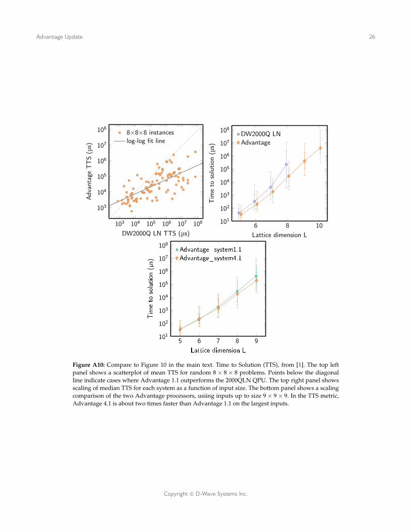
Figure A10: Compare to Figure 10 in the main text. Time to Solution (TTS), from [1]. The top leftpanel shows a scatterplot of mean TTS for random 8× 8× 8 problems. Points below the diagonalline indicate cases where Advantage 1.1 outperforms the 2000QLN QPU. The top right panel showsscaling of median TTS for each system as a function of input size. The bottom panel shows a scalingcomparison of the two Advantage processors, usiing inputs up to size 9× 9× 9. In the TTS metric,Advantage 4.1 is about two times faster than Advantage 1.1 on the largest inputs.


the advantage system: performance update

Documents