the adriatic sea general circulation. part i: air–sea

1492 VOLUME 27J O U R N A L O F P H Y S I C A L O C E A N O G R A P H Y

q 1997 American Meteorological Society

The Adriatic Sea General Circulation. Part I: Air–Sea Interactions andWater Mass Structure

A. ARTEGIANI,* D. BREGANT,1 E. PASCHINI,* N. PINARDI,# F. RAICICH,1 AND A. RUSSO*

* Istituto di Richerche sulla Pesca Marittima, CNR, Ancona, Italy1 Istituto Talassografico di Trieste, CNR, Trieste, Italy

# Istituto per lo Studio delle Metodologie Geofisiche Ambientali, CNR, Bologna, Italy

(Manuscript received 3 March 1995, in final form 5 March 1996)

ABSTRACT

A comprehensive historical hydrographic dataset for the overall Adriatic Sea basin is analyzed in order todefine the open ocean seasonal climatology of the basin. The authors also define the regional climatologicalseasons computing the average monthly values of heat fluxes and heat storage from a variety of atmosphericdatasets. The long term mean surface heat balance corresponds to a heat loss of 19–22 W m22. Thus, in steadystate, the Adriatic should import about the same amount of heat from the northern Ionian Sea through the OtrantoChannel. The freshwater balance of the Adriatic Sea is defined by computing the average monthly values ofevaporation, precipitation, and river runoff, obtaining an annual average gain of 1.14 m. The distribution ofheat marks the difference between eastern and western Adriatic areas, showing the winter heat losses in differentparts of the basin.

Climatological water masses are defined for three regions of the Adriatic: (i) the northern Adriatic whereseasonal variations in temperature penetrate to the bottom; deep water (NAdDW) with st . 29.2 kg m23 isproduced and salinity is greatly affected by river discharges; (ii) the middle Adriatic where a pool of modifiedNAdDW is stored during the summer season after being renewed in winter and modified Levantine IntermediateWater (MLIW) intrudes from the southern regions between spring and autumn; and (iii) the southern Adriaticwhere homogeneous water properties are found below 150 m (the local maximum depth of the seasonal ther-mocline) and a different deep water mass (SAdDW) is found with st . 29.1 kg m23, T ø 13.58C, and S ø 38.6psu. Due to river runoff waters, the surface layers of all three regions are freshened during the spring–summerseasons. The vertical distributions of dissolved oxygen vary quantitatively in the three regions showing a spring–summer subsurface maximum due to the balance between phytoplankton growth in the euphotic zone and lowvertical mixing in the water column. This behavior can be reconciled with open ocean conditions except for thenorthernmost part of the Adriatic where well-mixed oxygen conditions prevail throughout the year.

Large interannual anomalies of both temperature and salinity are found at the geographical center of the basinin surface and deep waters (100 m).

1. Introduction

The Adriatic Sea (Fig. 1) is an elongated basin, withits major axis in the northwest–southeast direction, lo-cated in the central Mediterranean, between the Italianpeninsula and the Balkans. Its northern section is veryshallow and gently sloping, with an average bottomdepth of about 35 m. The middle Adriatic is 140 m deepon average, with the two Pomo Depressions reaching260 m. The southern section is characterized by a widedepression more than 1200 m deep. The water exchangewith the Mediterranean Sea takes place through theOtranto Channel, whose sill is 800 m deep.

The eastern coast is generally high and rocky, whereas

Corresponding author address: Dr. Fabio Raicich, Istituto Speri-mentale Talassografico, CNR,Viale Romolo Gessi 2, I-34123 Trieste,Italy.E-mail: [email protected]

the western coast is low and mostly sandy. A largenumber of rivers discharge into the basin, with signif-icant influence on the circulation, particularly relevantbeing the Po River in the northern basin, and the en-semble of the Albanian rivers in the southern basin.

Studies of the Adriatic Sea started in the early eigh-teenth century, although a few observations are reportedearlier, and essentially concerned the coastal biologicalphenomenology, whereas open-sea observations beganin the nineteenth century. Several aspects of such re-search have been reported by many authors in the past,so that more details can be found in their papers(D’Ancona and Picotti 1958; Pigorini 1968; Trotti 1969;Buljan and Zore-Armanda 1976; Zavodnik 1983; Ar-tegiani et al. 1993).

Among those activities, the most significant contri-bution to the knowledge of the physical characteristicsof the basin was provided by the series of seasonalcruises made by the Permanent Italian–Austrian Com-mission in the years 1911–14 (R. Comitato Talasso-

AUGUST 1997 1493A R T E G I A N I E T A L .

FIG. 1. Adriatic Sea coastline and topography. Lines a and b define the northern, middle, and southern subbasins.

grafico 1912, 1913, 1914; Bruckner 1912, 1913, 1915).The results from these early cruises defined the basicknowledge of the basin phenomenology and the startingpoint for subsequent investigations up to the beginningof the 1980s.

Between the two world wars relevant contributionsdid not occur, although both Italian and Yugoslav re-searchers continued the observations and studies. SinceWorld War II there has been an increasing amount ofresearch, starting with Yugoslav surveys in 1947 (Buljanand Marinkovic 1956) and the Italian cruise of 1955(D’Ancona and Picotti 1958). The research was stim-ulated also by environmental problems induced by theoccurrence of anomalous phenomena, like strong stormsurges, intense algal blooms, and the presence of ge-latinous masses.

The large amount of data collected enabled the re-

searchers to outline, even if not always in a satisfactorymanner, some basic processes, such as the dense waterformation and the role of river discharges. Most of theanalysis has been performed in the northern basin (Fran-co 1970, 1972, 1982), so that its phenomenology isrelatively well known, compared to that of the middleand, especially, the southern basin (Artegiani et al.1993).

Here we analyze the hydrochemical dataset composedof almost all data collected from the beginning of thecentury to the early 1980s for the entire Adriatic Sea.This allows us to infer the structure of the general cir-culation of the overall basin. In Part I of the paper weanalyze the air–sea interaction budgets and the watermass structure of the basin. In Part II (Artegiani et al.1997) we describe the horizontal circulation features. Insection 2 of Part I we define the air–sea heat and mo-


FIG. 2a. Maps of February, May, August, and November average air temperature (8C) from the NMC dataset at 1000 hPa.

mentum fluxes for the overall region, classify the sea-sons on the basis of the Adriatic overall heat storage,and determine the fresh water balance. The dataset isdescribed in section 3, and we classify the water massesand the oxygen distribution in section 4. In section 5we describe the seasonal variations of water massesalong some selected vertical sections. Interannual vari-ability is analyzed at the available stations in section 6.Finally, conclusions are presented in section 7.

2. Atmospheric conditions, season definition, heat,and freshwater budgets

Here we give a climatological description of the at-mospheric conditions over the basin, and their effect interms of heat exchange and storage. One of the datasets

used was obtained from the National MeteorologicalCenter (renamed the National Centers for Environmen-tal Prediction). It consists of 12-h operational analysisfields at 1000 hPa, with 18 3 18 spatial resolution, forair temperature, relative humidity, and wind speed forthe period January 1980–December 1988. The originaldataset has been averaged to produce climatologicalmonthly mean values of the variables, shown in Figs.2a–c for the months of February, May, August, andNovember, which may be regarded as representative ofeach season.

Air temperature (Fig. 2a) exhibits seasonal fluctua-tions of about 208C over the entire basin. A longitudinalgradient prevails in the northernmost section, whereasa transverse gradient is dominant in the middle andsouthern Adriatic. The north–south temperature differ-


FIG. 2b. Maps of February, May, August, and November average relative humidity (%) from the NMC dataset at 1000 hPa.

ence ranges from about 3.58C in May to about 78C inNovember.

Relative humidity (Fig. 2b) is generally higher in thenorthern section and in the colder seasons, mainly as aconsequence of lower air temperature. The winter fieldis relatively homogeneous, whereas a significant lon-gitudinal gradient exists in the northern section in springand summer. A relative humidity minimum is presentin all seasons in the southern section.

The main characteristic of NMC wind data (Fig.2c) is a prevailing westerly component in all seasons;however, the two other datasets examined, Hellermanand Rosenstein (1983) and May (1982), exhibit adominant easterly component, at least over the north-ern and middle Adriatic, in agreement with the fre-

quent observations of northeasterly and southeasterlywinds made at most of the coastal meteorological sta-tions. In Fig. 2d February and November maps ofHellerman and Rosenstein’s and May’s data are shownfor comparison. We believe that the climatologicalNMC wind field is too zonal over this region andshows smaller intermonthly variations than the otherclimatological datasets; however, it is a dataset thatprovides consistent wind and temperature fields overthe area.

The adopted monthly mean cloudiness fields comefrom the Comprehensive Ocean Atmosphere Data Set(COADS). Cloudiness varies approximately betweentwo-tenths in July and six-tenths in January and Feb-ruary and is rather uniformly distributed over the whole


FIG. 2c. Maps of February, May, August, and November average wind speed (m s21) from the NMC dataset at 1000 hPa.

basin, the standard deviation associated with the spatialmean being about 10%.

Figure 2e shows the average fields of total heat fluxresulting from the May dataset (May 1986) for selectedmonths representing each season, namely, February,May, August, and November. We decided to display theMay dataset since it covers the entire basin, while theCOADS cloudiness dataset does not include some coast-al areas. A strong cooling occurs everywhere in No-vember, particularly in the northern region, while inFebruary the maximum heat loss is found in the middleAdriatic close to the western coast. In May a transversegradient is present, while in August a longitudinal gra-dient occurs in the northern and middle regions. Themaximum heat losses along the Italian coastline during

winter–spring months may support the conclusion thatthe western Adriatic coastal areas are dominated bydownwelling processes. This conclusion is also sup-ported by the presence of downwelling-favorable north-erly winds in winter and spring.

We have computed the climatological monthly heatbudget at the sea surface by means of the bulk formulasselected by Castellari et al. (1997, manuscript submittedto J. Mar. Res., hereafter referred to as CPL97) (see theappendix), using the atmospheric data described above.The monthly mean sea surface temperature fields areobtained from our hydrological dataset and will be dis-cussed later. To verify that the NMC wind pattern didnot affect our heat budget computations, we used allthree climatological wind datasets described above


FIG. 2d. Comparison between wind speeds (m s21) from Hellerman and Rosenstein (HR, left) and May (right).

(NMC, Hellerman and Rosenstein, and May). As wecan see in Fig. 3, the differences in wind direction didnot appreciably change the heat budget calculations.

Table 1 summarizes each heat budget componentcomputed by means of the NMC air temperature, rel-ative humidity, and wind data. We see that latent andlongwave radiation heat fluxes dominate the balancetogether with the shortwave incoming solar radiation.The annual average of the NMC heat budget is about219 6 10 W m22. For a comparison, we have alsocomputed the same quantities from the May dataset (Ta-ble 2). The annual average of May total heat flux is 222W m22 (no statistical error has been reported), which iscompatible with the value obtained from the fluxes sum-

marized in Table 1. Significant differences can be seenin the comparison of individual monthly values of theflux components, such as the summer values of the latentheat flux. This can be partly explained as follows: (i)the datasets cover different periods, since May usedobservations from 1945 to 1984, while we used atmo-spheric data for the period 1980–88 and sea surfacetemperatures for the periods 1911–14 and 1947–83; (ii)May first computed the fluxes from each individual ob-servation and subsequently calculated the spatial andtime averages, while the scarcity of available obser-vations forced us to use the space and time averagedvalues of the observations directly in the bulk formulas.Furthermore, we decided to use different bulk formulas


FIG. 2e. Maps of February, May, August, and November average surface total heat flux (W m 22) from May (1986). The contour intervalis 10 W m22 and the dashed lines indicate negative values.

than May and this may affect the estimates of individualterms (CPL97).

The negative annual average of the surface heat fluximplies that in steady-state conditions the Adriatic im-ports heat from the Mediterranean. This is expected dueto the deep-water formation processes occurring in thewinter and the known outflow–inflow system at Otranto(Ferentinos and Kastanos 1988; Michelato and Kova-cevic 1991). Warmer surface waters enter at Otranto,while at depth there is a net outflow of cold deep waters.Due to data paucity, the evaluation of heat transportfrom the hydrographic data would not be reliable andwe leave this question for future studies.

In order to arrange our hydrographic dataset on a

seasonal basis, we have defined the ‘‘ocean’’ seasonsaccording to Anati (1977). His method is based on thecomputation of the climatological heat storage in thetop layer, where the atmospheric influence mostly oc-curs. The definition of relative heat storage (HS) is takenfrom Hecht et al. (1985):

0DHS 5 c r(T 2 T ) dz if H , DE p 0H

2H

0

HS 5 c r(T 2 T ) dz if H $ D, (1)E p 0

2D

where H is the actual water column depth, D is the


FIG. 3. (Upper left) Monthly mean heat flux at the surface computedwith the NMC (3), Hellerman and Rosenstein’s (M), and May’s (V)wind datasets, but other parameters only from NMC data. The totalheat flux computed by May (1986) (#) is also displayed for com-parison. (Upper right) Monthly mean relative heat storage for the top50-m layer. (Lower) Monthly means of precipitation, evaporation,and river runoff, together with freshwater budget displayed below.

maximum water depth considered, cp the specific heatat constant pressure, r the in situ density, T the watertemperature, and T0 an arbitrary reference temperature.In our computations D 5 50 m, cp has been computedaccording to Fofonoff and Millard (1983), r and T havebeen derived from our dataset, and T0 5 108C. For thepurpose of seasonal definition, we are not interested inthe actual heat storage values, but rather in its annual

cycle, which turns out to be almost insensitive to Dgreater than 50 m and less than 150 m. The relative heatstorage is shown in Fig. 3. Two extreme seasons can beclearly distinguished, namely, winter from January toApril, and summer from July to October. We can alsodefine the two transition seasons: spring, consisting ofMay and June, and autumn, consisting of November andDecember.


TABLE 1. Monthly surface heat flux components from NMC airtemperature, relative humidity, and wind data, COADS cloud dataand sea surface temperature of our dataset: QS is the incident solarradiation flux, QB the backward radiation flux, QH the sensible heatflux, QE the latent heat flux, and Q the total heat flux (see the ap-pendix). All units are in W m22; the annual average is 219 6 10 Wm22.

Month QS QB QH QE Q

JanFebMarAprMayJunJulAugSepOctNovDec

5181

131198238282302256187119

6446

287 6 2288 6 2280 6 2280 6 3263 6 3259 6 5250 6 6249 6 6256 6 5276 6 4284 6 3293 6 2

250 6 2251 6 2228 6 3212 6 3

5 6 26 6 17 6 15 6 16 6 1

210 6 1232 6 3259 6 3

2135 6 52134 6 52115 6 62103 6 7264 6 11243 6 11230 6 8225 6 7238 6 11

2120 6 132133 6 72170 6 6

2221 6 72192 6 7292 6 7

3 6 9116 6 12186 6 12229 6 11188 6 9

99 6 13287 6 15

2185 6 92275 6 8

TABLE 2. May’s monthly surface heat flux components: QS is theincident solar radiation flux, QB the backward radiation flux, QH thesensible heat flux, QE the latent heat flux, and Q the total heat flux(see the appendix). All units are in W m22; the annual average is222 W m22

Month QS QB QH QE Q


6699

153201251283296254196133

7755

276273269267261259264266269270271270

2482362162922

02226

212213230238

21482123288274261269

210521172125211221352141

22072133220

52128155124

65210262

21592193

TABLE 3. Freshwater balance components: E is evaporation, Pprecipitation, and R runoff. All units are in meters.

Month E P R E 2 (P 1 R)


0.14 6 0.010.14 6 0.010.12 6 0.010.11 6 0.010.07 6 0.010.05 6 0.010.03 6 0.010.03 6 0.010.04 6 0.010.13 6 0.010.14 6 0.010.18 6 0.01

0.11 6 0.050.09 6 0.040.09 6 0.040.07 6 0.030.07 6 0.020.05 6 0.020.03 6 0.010.04 6 0.020.08 6 0.020.12 6 0.040.14 6 0.050.14 6 0.06

0.12 6 0.050.12 6 0.050.12 6 0.050.14 6 0.060.13 6 0.050.11 6 0.040.06 6 0.030.05 6 0.020.06 6 0.030.08 6 0.030.13 6 0.050.15 6 0.06

20.08 6 0.0720.07 6 0.0620.09 6 0.0620.10 6 0.0620.13 6 0.0620.12 6 0.0520.06 6 0.0320.06 6 0.0320.10 6 0.0420.08 6 0.0520.13 6 0.0720.11 6 0.08

Year 1.17 6 0.03 1.02 6 0.12 1.29 6 0.16 21.14 6 0.20

The relationship between the heat storage and totalsurface heat flux Q can be written as follows:

2(HS) 5 Q 2 v · =(HS) 2 K ¹ (HS)t H

1 w HSz 2 K c rT z . (2)z52D V p z z52D

The advective term in the right-hand side is dominatedby its horizontal components v, since the vertical ve-locity w is much smaller than the horizontal velocityand since its influence has been reduced due to the ver-tical integration. If we now integrate horizontally andmake these approximations, Eq. (2) becomes

(HS) dA 5 Q dA 2 v ·nHS dlEE t EE EA A O

1 K =(HS)·n dl, (3)H EO

where A is the surface of the Adriatic basin and O itsboundary across the Otranto Channel. The upward ordownward heat flux at the base of the seasonal ther-mocline layer is considered to be negligible when thehorizontal average is carried out. If the right-hand sideof Eq. (3) consisted only of Q, then Q and HS wouldbe exactly 908 out of phase. Comparing Fig. 3 upper-left and upper-right panels, it can be seen that both theHS increase in winter–spring and decrease in sum-mer–autumn are faster than expected if HS were con-trolled only by Q; therefore, advection and diffusionthrough the Otranto Channel affect the heat storage sig-nificantly. This is again evidence that the inflow of sur-face and intermediate waters through the Otranto Chan-nel is important for the overall heat budget of the basin.

We have computed the monthly mean freshwater bal-ance and its components evaporation (E), precipitation(P), and river runoff (R). Figure 3 and Table 3 sum-marize these results. Evaporation data and standard de-viations have been determined from the latent heat flux-

es of Table 1. Precipitation has been extracted from theclimatology developed by Legates and Willmott (1990),who estimated that P is affected by a 40% standarddeviation on average. The river discharges have beentaken from Raicich (1994), who estimated the standarddeviation to be 30%–60%, which is compatible with theestimate for P given above. The error bars for the totalwater budget, shown in Fig. 3, are then obtained fromthe individual standard deviations. The three compo-nents of the freshwater balance are of the same orderof magnitude, with negative values of E 2 (P 1 R) inall the months, and a total fresh water gain of 1.14 60.20 m yr21. The precipitation budget appears to beoverestimated probably due to the lack of open sea ob-servations, since precipitation is expected to be lowerin the open ocean than along the coasts. We havechecked the precipitation data utilized with those ob-served at coastal stations; it turns out that the Legatesand Willmott (1990) data appear to be overestimated asmuch as 50% along the southeastern coastlines. How-ever, computing the average annual water budget E 2(P 1 R) from the coastal data, the water balance remainsnegative.


FIG. 4. Yearly cast distribution.

TABLE 4. Details on the historical Adriatic dataset: C represents the number of casts reported in each reference; CT the number of castswith temperature data; DT the number of temperature data; CS, DS, the same for salinity; and CO, DO the same for dissolved oxygen.

Reference C CT DT CS DS CO DO

Artegiani and Azzolini (1980)Artegiani et al. (1981)Brasseur et al. (1993)Bruckner (1912, 1913, 1915)Buljan and Zore-Armanda (1966, 1979)

107115850350

1062

107115832350

1061

640450

449223458042

107115832348

1051

644455

421223407955

40115338

92322

284450

1669174

2668Cescon and Scarazzato (1979)ENEA (1990)Franco (1970, 1972, 1982)Hydrographic Inst. of the Yugoslav Navy (1982)Inst. za Oceanologiju i Ribarstvo, Split (1985)

523583335154

29

523583335154

29

1974251313981566

175

523581335154

29

1971249914151566

171

392—

320133

16

1341—

13551283

29Levitus (1982)P. Malanotte-Rizzoli (1972, pers. comm.)Mosetti and Lavenia (1969)R. Comitato Talassografico (1912, 1913, 1914)Trotti (1969)Zore-Armanda et al. (1991)

12973

300471171291

12973

300470171286

808431

1788405012392866

12973

300470171285

816427

1787405012382809

4973—

373171239

348425—

158711732419

Total 5543 5518 34 777 5503 34 355 2673 15 205

3. The hydrographic dataset

The hydrographic dataset comprises measurements oftemperature, salinity, and dissolved oxygen taken bybottle sampling in the periods 1911–14 and 1947–83.The yearly station distribution is shown in Fig. 4. After1983 all the measurements were made with CTD casts,which will be considered in a following paper. All thestations with less than 15-m bottom depth and otherslocated close to the eastern coast have been omitted fromour analysis since we wanted to eliminate water prop-erties strongly affected by coastal processes. The re-sulting dataset comprises a total of 5543 stations (Table4), 5518 of which include temperature, 5503 includesalinity, and 2673 include dissolved oxygen. Figure 5shows the spatial distribution of these stations.

Generally, observations were made at the followingdepths: 0, 5, 10, 20, 30, 40, 50, 75, 100, 150, 200, 250,300, 400, 500, 600, 800, 1000, and 1200 m. If a valuewas not available for one of the above depths, linearinterpolation between adjacent values was performed.

Most of the data (85%–90%) was obtained from hy-drological casts performed by Nansen and Niskin bottles(or other analogous bottles) equipped with protected andunprotected reversing thermometers. The uncertainty onthe percentage is due to the fact that some authors usedboth reversing thermometers and in situ probes, but theydid not specify in their papers from which instrumentthe data were obtained.

Until 1960 salinity data were obtained by means of theMohr–Knudsen titration method, using the Eau de MerNormale as standard. After 1970, all of the salinity de-terminations were made from laboratory salinometers cal-ibrated with the same standard. Between 1960 and 1970,many authors used both methods in conjunction. The au-thors rarely gave confidence limits of the experimentaldata. We can assume that the approximate temperatureuncertainty is 0.028C and for salinity it is 0.02 psu fortitration and 0.005 psu for the conductivity method. Moredetails can be found in U.S. Navy (1968).

The analytical method usually adopted for the dis-solved oxygen determination is outlined by Winkler(1888). Various adaptations, essentially concerning thestandardization procedures, have been reported by Ja-cobsen (1921), Vercelli and Picotti (1926), Thompsonand Robinson (1939), and Koide, quoted in Trotti(1969). After 1960 the methodology follows the sug-gestions proposed by Strickland and Parsons (1960),except for some improvements in the standards as re-ported by Grasshoff et al. (1983). The authors rarelyreport experimental accuracy and sensitivity limits;therefore, we rely on the description of each method.Generally, both accuracy and sensitivity cannot be con-sidered better than 0.05 ml l21.

The following quality checks were carried out on theraw dataset: (i) geographical position check; (ii) checkthat the same station did not appear in different datasets;(iii) climatological check, which consists of the follow-


FIG. 5. Spatial cast distribution.

ing: Since the data exhibit large spatial and temporalvariability, the Adriatic Sea was divided into six areasfor which the monthly means and standard deviationswere calculated. For temperature and salinity the mea-surements were averaged in the following layers: 0–9m, 10–29 m, 30–99 m, 100–269 m, 270–599 m, andfrom 600 m to the bottom. All of the values that departedfrom the mean by more than three standard deviationswere rejected. For dissolved oxygen every depth wasexamined separately in each area. All of the values out-side the range 4.5–6 ml l21 and departing from the meanby more than three standard deviations were rejected.This procedure was repeated three times, discarding 202values of dissolved oxygen.

On the basis of the climatological averages of thesedata, we defined three regions with homogeneous phys-ical water properties: the northern Adriatic extending upto the 100-m isobath in the south, the middle Adriaticcharacterized by the Pomo Depressions up to the Viestetransect, and the southern Adriatic up to the OtrantoChannel. The northern Adriatic region is slightly largerthan previously defined (Orlic et al., 1992) because wefound that the water properties are homogeneous whencalculated according to the regional boundaries definedhere.

4. Water mass structure

a. Temperature and salinity

Figures 6, 7, and 8 show the climatological profilesfor temperature and salinity and the climatological TSdiagrams obtained from our dataset for the three regions

defined above. In the following we describe the watermass characteristics of the three regions separately.

In the northern Adriatic the entire water column ex-hibits an evident seasonal thermal cycle. A well-de-veloped thermocline is present in spring and summerdown to 30-m depth, whereas a significant cooling be-gins close to the surface in autumn when the bottomtemperature reaches its maximum value, probably dueto increased vertical mixing and intrusion of middleAdriatic waters. Only in winter the cooling of thewhole water column occurs; in this season temperaturegenerally increases down to the bottom, but the watercolumn stability is preserved due to an associated in-crease of salinity at depth. The freshwater effect isclearly seen in spring and summer due to the increasedrunoff and the increased water column stratification.From these averaged temperature and salinity profilesthere is no evidence of modified Levantine Interme-diate Water (MLIW) (described later for the middleAdriatic) in the northern basin. We can recognize aseasonal layer of northern Adriatic surface water(NAdSW), which corresponds to low salinities and rel-atively high temperatures of the summer, and a north-ern Adriatic deep water (NAdDW) layer, which iscooled and renewed in winter. From Fig. 8a we candefine the NAdDW having average characteristics ofT 5 11.35 6 1.408C, S 5 38.30 6 0.28 psu, and densityst . 29.2 kg m23.

In the middle Adriatic the spring–summer thermo-cline is formed down to a depth of 50 m. In the layerfrom 50 to 150 m the seasonal temperature changes arestill observed. The MLIW in this region is defined by


FIG. 6. Seasonal climatological profiles of temperature (8C) for (a)northern, (b) middle, and (c) southern Adriatic for winter (M), spring(V), summer (#), and autumn (n).

FIG. 7. Seasonal climatological profiles of salinity (psu) for (a)northern, (b) middle, and (c) southern Adriatic for winter (M), spring(V), summer (#), and autumn (n).

waters with salinity S . 38.5 psu below 50 m. The surfacewaters are freshened during spring and summer, as in thenorthern Adriatic, due to river runoff. Hence, the riverrunoff also exceeds evaporation during summer in the mid-

dle Adriatic. The Pomo Depressions are the only areasdeeper than 150 m. They are filled with a deep water mass,which exhibits some seasonal changes. The middle Adri-atic deep water (MAdDW) has relatively low average tem-perature (T 5 11.62 6 0.758C) and substantially higher


FIG. 8. Climatological T–S diagram for (a) northern, (b) middle,and (c) southern Adriatic for winter (M), spring (V), summer (#),and autumn (n). The solid lines indicate st.

average salinity (S 5 38.47 6 0.15 psu) than the NAdDWbut the density is still st . 29.2 kg m23, Fig. 8b. If thiswater originates from the winter NAdDW moving south-ward, then it experiences substantial mixing and entrain-ment, transforming the NAdDW into MAdDW. Fromspring to autumn, the MAdDW is the coldest bottom watermass in all the Adriatic basin.

In the southern Adriatic the seasonal thermocline ex-tends down to approximately 75 m. The seasonal cycleof the surface waters is driven by the fresh coastal watersas seen by the decrease in salinity in all seasons and theaugmented minimum during spring and summer. From150 m to the bottom, Mediterranean open sea conditionsare found since the water is almost homogeneous, witha relatively weak seasonal signal down to 300 m, mod-ulated by MLIW advection and mixing. In this regionthe MLIW is defined by S . 38.6 psu and T . 13.58C,with a layer between 150 and 400 m. The southern Adri-atic deep water (SAdDW) again has different averagecharacteristics from NAdDW and MAdDW. It is definedby T 5 13.16 6 0.308C and S 5 38.61 6 0.09 psu,corresponding to st . 29.1 kg m23 (Fig. 8c). Thus, thiswater is considerably warmer and saltier compared toNAdDW and MAdDW so that it probably comprises amixture of MLIW and local surface waters (Ovchinnikovet al. 1985; Roether and Schlitzer 1991).

To quantify the variability of the hydrological param-eters we use the observed standard deviations (STD)associated with the climatological mean values. TheSTDs depend mainly on the seasonal and interannualfluctuations but are also strongly affected by the numberof observations used in the computations.

In the northern Adriatic temperature STD ranges from0.88–1.18C near the bottom (with a minimum value inspring and a maximum in winter) to 2.18–2.68C near thesurface (a minimum in winter and maximum in autumn).In spring and summer the maximum respective STDs2.28 and 2.48C occur at 20 m as a consequence of thevariability in the thickness of the seasonal surface mixedlayer. In the middle Adriatic the temperature STD is0.68–0.88C near the bottom and ranges between 1.18Cin winter and 2.48C in spring near the surface. In thisregion the highest variability in the summer occurs at20-m depth (STD 5 1.98C), as in the northern basin.In the southern Adriatic, the bottom STD is about 0.28C,while at the surface it ranges between 1.18C in winterand 2.58C in spring. Again the maximum summer STDoccurs at 20 m (STD 5 2.38C).

The salinity STD always decreases from the surfaceto the bottom in all three subbasins. In the NorthernAdriatic the lowest STDs range from 0.1 psu in winterand 0.3 psu in summer, near the bottom, and the highestfrom 2.1 psu in autumn to 3.2 psu in spring at thesurface. The middle Adriatic winter salinity exhibits thelowest variability, with STD of 0.1 psu near the bottomand 0.5 at the surface, while the other seasons are similarto each other, with bottom STD of 0.2 psu and surfaceSTD of 0.9–1.1 psu. In the southern Adriatic the bottom


FIG. 9. Climatological profiles of dissolved oxygen (ml l21) for (a) the northern Adriatic withbottom depth less than or equal to 50 m, (b) northern Adriatic with bottom depth greater than 50m, (c) middle Adriatic, (d) southern Adriatic for the entire water column, and (e) southern Adriaticfor the upper 300 m. Symbols indicate winter (M), spring (V), summer (#), and autumn (n).

STD is less than 0.1 psu, whereas at the surface it rangesbetween 0.3 psu in summer and 0.8 psu in spring.

b. Dissolved oxygen

The whole Adriatic Sea is a well-oxygenated basin.The dissolved oxygen profiles (Fig. 9) show that in thewarmer seasons a relatively low concentration layer ispresent just near the sea surface, due to oxygen equil-

ibration with the atmosphere. During spring and summera subsurface maximum is formed in the euphotic zone,between approximately 10 and 50 m, due to biologicalactivity that results in a net production of oxygen nearthe pycnocline after the density stratification of the wa-ter column has become established. In autumn and win-ter ventilation at the surface and water column mixingcreate a more homogeneous oxygen distribution.

In the northern Adriatic we noticed a qualitatively


FIG. 10. Spatial cast distribution along selected cross sections. The Pelagosa area is indicatedby the box on the Vieste section.

FIG. 11. Sigma-t anomaly (kg m23) vertical distribution along theAncona, Pescara, and Vieste sections for winter.

different shape of the average oxygen profiles with re-spect to middle and southern Adriatic conditions, andthus we subdivided the northern Adriatic in two sub-regions. The first corresponds to the area shallower than50 m, called NA-I region, and the second correspondsto the remaining part, called NA-II region. In Fig. 9afor the NA-I region, we show that in all seasons thereis no subsurface oxygen maximum except for springwhen we observe it at 5–10 m. The NA-II region bycontrast shows maximum subsurface values for springand summer as for the middle and southern Adriaticcases. Naturally, the highest values of oxygen for theentire basin are reached during winter in the NA-I re-gion. Thus, the NA-I region is clearly that part of thenorthern Adriatic basin that is characterized by shallowsea dynamics evidenced by the increased mixingthroughout the water column, even during summer. Incontrast deep-sea conditions are found in the NA-II re-gion where oxygen profiles look similar to those of themiddle Adriatic. Hence, the pelagic lower trophic sys-tem dynamics (i.e., nutrients and phytoplankton) are ex-pected to be different in NA-I and NA-II regions basedon different vertical distributions of oxygen.

In the middle Adriatic the oxygen concentration de-creases from the euphotic zone (50 m) down to thebottom, while in the southern Adriatic a minimum isfound at 150–250 m due to the organic matter oxidation.Below this minimum, the oxygen concentration slightlyincreases down to the bottom. The relative minimum at40–50 m in autumn and winter in the southern Adriatic(Fig. 9d) could be due to fewer observations relative tothe levels above and below those depths.


FIG. 12. Sigma-t anomaly (kg m23) vertical distribution along theAncona, Pescara, and Vieste sections for spring.

FIG. 13. Salinity (psu) vertical distribution along the Ancona, Pes-cara, and Vieste sections for spring.

An average basin value of dissolved oxygen is ap-proximately 5.5 ml l21, and we used standard deviations(STD) to describe the oxygen variability. In the northernAdriatic the lowest variability in the oxygen concentra-tion occurs near the bottom with STD ranging from 0.1ml l21 in autumn and 0.4 ml l21 in summer, while thehighest STDs occur at the surface with values of 0.5–0.6 ml l21 in all seasons except for summer when thehighest STD of 0.9 ml l21 is found at a depth of 30 m.In the remaining part of the Adriatic Sea STD exhibitsneither significant seasonal changes nor a clear depen-dence on the depth. In the middle Adriatic the STDrange is 0.3–0.6 ml l21, and in the southern basin wherethe number of observations is relatively low along theentire water column the STD mainly ranges between0.2 and 0.4 ml l21.

Usually, the oxygen saturation percentage does notdrop below 75%, whereas maximum values can begreater than 110%. In the northern Adriatic hypoxia(mostly deduced from phenological observations butrarely measured) can occur under particular conditionsassociated with specific phenomenology. Such occur-rences cannot be recognized in our mean values due tothe sporadic nature of these events.

5. Vertical sections

In this section we describe the seasonal variability intemperature, salinity, and density for five lateral sec-tions. The station locations that define the sections areshown in Fig. 10. We see that along these five sectionsthe stations accumulate so that it is possible to defineseasonal mean properties along an average position,which we call a section. The sections are called Ancona,Pescara, Vieste, Bari, and Otranto after the nearby Ital-ian cities.

a. Ancona, Pescara, and Vieste sections

The Ancona section is representative of the transitionarea between the northern and middle Adriatic regions.The Pescara section characterizes the middle Adriatic,while the Vieste section represents the transition areato the southern Adriatic.

The density distribution on these three sections isshown in Fig. 11 for winter and Fig. 12 for spring. Twoimportant characteristics of the northern and middleAdriatic winter circulation are evident from Fig. 11; (i)the coastal waters affected by river runoff are confinedalong the continental shelf and escarpments of both


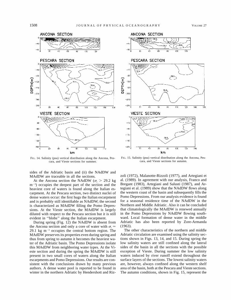
FIG. 14. Salinity (psu) vertical distribution along the Ancona, Pes-cara, and Vieste sections for summer.

FIG. 15. Salinity (psu) vertical distribution along the Ancona, Pes-cara, and Vieste sections for autumn.

sides of the Adriatic basin and (ii) the NAdDW andMAdDW are traceable in all the sections.

At the Ancona section the NAdDW (st . 29.2 kgm23) occupies the deepest part of the section and theheaviest core of waters is found along the Italian es-carpment. At the Pescara section, two distinct nuclei ofdense waters occur: the first hugs the Italian escarpmentand is probably still identifiable as NAdDW; the secondis characterized as MAdDW filling the Pomo Depres-sions. At the Vieste section, the MAdDW is largelydiluted with respect to the Pescara section but it is stillevident in ‘‘blobs’’ along the Italian escarpment.

During spring (Fig. 12) the NAdDW is absent fromthe Ancona section and only a core of water with st ø29.1 kg m23 occupies the central bottom region. TheMAdDW preserves its properties even during spring andthus from spring to autumn it becomes the heaviest wa-ter of the Adriatic basin. The Pomo Depressions isolatethis MAdDW from neighboring water types. At the Vi-este section and during the spring the MAdDW is stillpresent in two small cores of waters along the Italianescarpments and Pomo Depressions. Our results are con-sistent with the conclusions drawn by many previousauthors. A dense water pool is reported to be found inwinter in the northern Adriatic by Hendershott and Riz-

zoli (1972), Malanotte-Rizzoli (1977), and Artegiani etal. (1989). In agreement with our analysis, Franco andBregant (1983), Artegiani and Salusti (1987), and Ar-tegiani et al. (1989) show that the NAdDW flows alongthe western coast of the basin and subsequently fills thePomo Depressions. From our analysis evidence is foundfor a seasonal residence time of the NAdDW in theNorthern and Middle Adriatic. Also it can be concludedthat climatologically the MAdDW is renewed annuallyin the Pomo Depressions by NAdDW flowing south-ward. Local formation of dense water in the middleAdriatic has also been reported by Zore-Armanda(1963).

The other characteristics of the northern and middleAdriatic circulation are examined using the salinity sec-tions shown in Figs. 13, 14, and 15. During spring thelow salinity waters are still confined along the lateralsides of the basin in all the sections with the possibleexception of Vieste. During summer the low salinitywaters induced by river runoff extend throughout thesurface layers of the sections. The lowest salinity watersare, however, always confined along the western shelfarea of the basin, both at the Pescara and Vieste sections.The autumn conditions, shown in Fig. 15, represent the


transition toward the wintertime regime with increasedgradients of salinity along the escarpments.

At intermediate depths between 50 and 150 m we candetect (in Figs. 13, 14, and 15) the presence of MLIW(S . 38.5 psu in the middle and S . 38.6 psu in thesouthern Adriatic) in all seasons except winter (notshown). The greatest intrusion of MLIW is evident inautumn, as shown by the large area enclosed by the38.5-psu isohaline in Fig. 15 for the Pescara and Viestesections. At the Ancona section the MLIW can be tracedon the eastern side of the section only during summerand autumn. The MLIW did not result from the averageclimatological profiles of Fig. 8a since the area occupiedby this high salinity water mass is relatively small andthe spatial average removes this signal.

b. Bari section

This section is representative of the central southernAdriatic. The winter conditions, shown in Fig. 16a, arecharacterized by low temperature and low salinity coast-al waters on the western shelf area of the Adriatic. Inthe deepest part of the section we find the SAdDW withT , 13.08C and S , 38.6 psu. These dense waters areprobably of local origin, in agreement with the resultsby Pollak (1951), Ovchinnikov et al. (1985), and Roeth-er and Schlitzer (1991), who indicate the southern basinas an area of SAdDW formation. Above the SAdDWthere is a thick transition layer with 13.0 , T , 13.58C,and the MLIW lies above that layer.

During spring (Fig. 16b), the MLIW is evident onlyon the eastern side of the basin and it exhibits patchinessat intermediate depths. The SAdDW is still evident atthe bottom while the surface waters have decreased theirsalinity in the first 50 m. Hence, we conclude again thatthe river runoff waters affect also the southern Adriaticsurface waters.

c. Otranto section

This section is shown in Fig. 17 for winter and springconditions. This is the route of exchange of waters withthe eastern Mediterranean, so that it is interesting totrace the deep water masses along the section.

During winter, the western side of the section alongthe escarpment is occupied by a very dense water char-acterized by T , 13.58C and S , 38.6 psu. The centraland eastern part of the section shows the presence ofMLIW (13.58 , T , 14.58C, S . 38.6 psu). TheSAdDW is evident as a small nucleus in the deepestpart of the section with T ø 13.58C and S ø 38.6 psu.

During spring the MLIW central core is shifted up-ward around 300 m, while during winter it is centeredaround 600 m. It is interesting to note that during springthe SAdDW seems to have cooled and freshened a littlewith respect to winter values. Thus, we conclude thatthe SAdDW could have mixed with MAdDW and/orthe heavy coastal waters seen along the western es-

carpment during winter. However, the paucity of datain this region of the Adriatic does not allow us to drawany definitive conclusions about mixing of different wa-ter masses in the Southern basin.

6. Interannual variability of time series

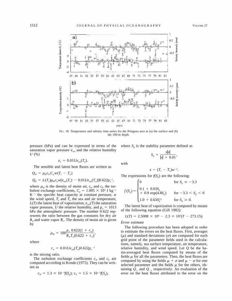
The entire dataset presented here contains few areaswith long time series. We choose to show the time seriesin a region of 36 3 41 km2 at the center of the Viestesection. This area is called Pelagosa after the nearbyisland. Between 1947 and 1983 we have temperatureand salinity data with the exception of 1951–52 and1973–74.

In Figs. 18a,b we show the area-averaged temperatureand salinity anomalies for the surface and 100-m depthafter the seasonal cycle has been removed. As expected,the temperature interannual variability is larger at thesurface, with maximum deviations of 48C, than at depth(deviations of 28C at 100 m). The analysis by means ofthe periodogram method (Stull 1988) reveals that theinterannual variability in temperature and salinity peaksat different periods. Temperature anomalies are domi-nated by fluctuations of high frequency (1–2 yr) andrelatively low frequency (12–13 yr) both at the surfaceand 100 m. The variance explained by the 1-yr and 2-yrfluctuations is about 10% at both levels, and the 12-yror 13-yr components explain about 7% of total varianceat the surface and 13% at 100 m. The variability ofsalinity anomalies is characterized by fluctuations ofintermediate frequency (3 and 6 yr), both at the surfaceand at 100 m. At 100 m a 12-yr fluctuation is also found,as for temperature at that depth. The 3-yr and 6-yr com-ponents explain about 9% and 18%, respectively, of thetime series variance at the surface, while at 100 m ap-proximately 15% of the total variance is explained bythe 12-yr component, 8% by the 6-yr component, and6% by the 3-yr component. Since 1970–71 we can de-tect a trend of increasing salinity and temperature butthe data are not sufficiently accurate to make conclu-sions about climatic changes (Zore-Armanda et al.,1991).

7. Conclusions

The work presented here describes the climatologicalwater mass and dissolved oxygen structure of the Adri-atic Sea. The dataset was collected and quality-con-trolled and a seasonal climatological analysis produced.A monthly analysis was not feasible because of the pau-city of data.

First, we studied the meteorology of the basin andthe air–sea interaction budgets. Several climatologicalwind datasets were compared and discussed and theclimatological heat budget of the basin computed bymeans of bulk formulas. The heat budget at the surfaceis dominated by the incoming shortwave heat flux bal-anced by longwave and latent heat energy losses. It was


FIG. 16. Temperature (8C, left) and salinity (psu, right) vertical distributions along the Barisection for (a) winter and (b) spring.

found that the basin has an overall long term heat lossof 19–22 W m22, which implies an import of heat fromthe northern Ionian through the Otranto Channel. Thelatter is shown to play an important role also in the heatstorage balance of the Adriatic basin. These climato-logical considerations show that the Adriatic is a heatengine like the overall Mediterranean, but it is a dilutionbasin since the freshwater balance implies an averagefreshwater gain of 1.14 m yr21.

The overall Adriatic basin is subdivided in three ar-eas: the Northern basin with shallow sea water masscharacteristics; the middle Adriatic, which is a transitionbasin but with some well-defined open sea character-istics (persistence of a pool of deep water during spring–summer seasons); and the Southern basin with open seawater mass characteristics below 150 m.

We have classified for the first time the water massesof the basin using climatological averages and verticalsections. The surface waters of all the three regionsundergo a clear temperature seasonal cycle with max-

imum values of temperature during summer and max-imum mixed layer depths during winter. The salt balanceof the surface layer is clearly affected by freshwaterriver runoff in all the three regions during spring andsummer. Fresher coastal waters are always separated anddistinguishable from open sea waters in all seasons. Wecan recognize the MLIW and deep waters spreadingpaths. The MLIW is defined by S . 38.5 psu in themiddle Adriatic and S . 38.6 psu in the subsurfacelayers of the southern Adriatic. Its maximum abundanceis reached during autumn where it occupies almost theentire water column in the middle and southern Adriatic.The MLIW intrusion can be detected also in the northernAdriatic, but from the climatology we have no evidenceof such a phenomenon, which seems to be rather lo-calized. To a first-order approximation the northernAdriatic seems to be dynamically independent of themiddle and southern Adriatic, however, it clearly influ-ences the dynamics of the other two regions through thesouthward movement of NAdDW.


FIG. 17. Temperature (8C, left) and salinity (psu, right) vertical dis-tributions along the Otranto section for (a) winter and (b) spring.

The deep waters of the Adriatic can be separated intotwo categories: the first, clearly formed in the northernAdriatic region, cool and relatively fresh, found in thenorthern and middle Adriatic, and the second of muchhigher temperature and salinity, in the southern Adriatic.It is our perception that vertical mixing between watermasses is an extremely powerful dynamical process inthe basin, especially as an explanation of the modifi-cation of NAdDW into MAdDW.

Acknowledgments. This research has been undertakenin the framework of the Mediterranean Targeted Project(MTP)—MERMAIDS II Project, and finished duringthe Mediterranean Targeted Project phase II—MATER.We acknowledge the support of the European Com-mission’s Marine Science and Technology Programme(MAST II and III), Contracts MAS2-CT93-0055 andMAS3-CT96-0051. We thank Dr. S. Castellari for guid-ance in the air–sea interaction modeling. We thank alsoDrs. J. Baretta, P. Radford, and M. Zavatarelli and Prof.

G. Mellor for helpful comments on the manuscript.Thanks are also due to Mr. P. Carini for his assistancein figure drawing.

APPENDIX

Heat Budget Computations

The computation of the net heat flux at the sea surfaceQ has been made by means of the bulk formulas (in SIunits), which will be summarized here. More details canbe found in CPL97. Here Q can be expressed as

Q 5 QS 2 QB 2 QH 2 QE,

where QS is the downward flux of solar radiation reach-ing the sea surface, QB the net longwave radiation fluxemitted from the sea surface, and QH and QE the sensibleand latent heat fluxes from the sea surface to the at-mosphere.

The incident solar radiation flux QS can be written as

QS 5 QTOT (1 2 0.38 C 2 0.38C2) (1 2 a),

where C is the fractional cloud cover and a is the oceansurface albedo, which depends on the solar altitude ac-cording to Payne (1972). The cloud attenuation factorwas proposed by Berliand (Budyko 1974).

Here QTOT is the sum of two components, the flux ofdirect radiation reaching the surface and the flux of ra-diation scattered downward by the atmosphere

Q 5 Q 1 QTOT DIR DIFF

seczQ 5 Q t ;DIR 0

Q 5 0.5[(1 2 A ) Q 2 Q ].DIFF a 0 DIR

Here Q0 is the solar radiation flux at the top of theatmosphere, z the zenith angle, QDIR is the fraction ofQ0 transmitted through the atmosphere (transmission co-efficient t 5 0.7), and QDIFF is computed under the hy-pothesis that the radiation scattering in clear sky occurshalf downward and half upward (Rosati and Miyakoda1988); the scattered radiation is the amount not reachingthe surface minus that absorbed by water vapor andozone (absorption coefficient Aa 5 0.09). The expres-sion for Q0 is

Q0 5 J0a22 cos(z)DF(f),

where J0 5 1.35 3 103 J m22 s21 is the solar constant,a the earth radius, and DF(f) the fraction of daylight.

The longwave radiation flux QB is computed by meansof Berliand’s formula (Simpson and Paulson 1979)

4 1/2 2Q 5 «sT (0.39 2 0.05e )(1 2 0.8C )B a a

31 4«sT (T 2 T ),a s a

where « 5 0.97 is the ocean longwave emissivity, s 55.67 3 1028 W m22 K24 the Stefan–Boltzmann constant,Ts and Ta the sea and atmosphere temperatures, and Cthe fractional cloud cover; ea is the atmospheric vapor


FIG. 18. Temperature and salinity time series for the Pelagosa area at (a) the surface and (b)the 100-m depth.

pressure (hPa) and can be expressed in terms of thesaturation vapor pressure esat and the relative humidityU (%)

ea 5 0.01Uesat(Ta).

The sensible and latent heat fluxes are written as

Q 5 r c C w(T 2 T )H M H p s a

21Q 5 L(T )r c w[e (T ) 2 0.01Ue (T )]0.622p ,E s M E sat s sat a a

where rM is the density of moist air, cH and cE the tur-bulent exchange coefficients, Cp 5 1.005 3 103 J kg21

K21 the specific heat capacity at constant pressure, wthe wind speed, Ts and Ta the sea and air temperature,L(T) the latent heat of vaporization, esat(T) the saturationvapor pressure, U the relative humidity, and pa 5 1013hPa the atmospheric pressure. The number 0.622 rep-resents the ratio between the gas constants for dry airRd and water vapor Rv. The density of moist air is givenby

p 0.622(1 1 r )a wr 5 100 ,M R T (0.622 1 r )d a w

where

rw 5 0.01Uesat(Ta)0.622pa21

is the mixing ratio.The turbulent exchange coefficients cH and cE are

computed according to Kondo (1975). They can be writ-ten as

cH 5 1.3 3 1023f(Sp); cE 5 1.5 3 1023f(Sp),

where Sp is the stability parameter defined as

szszS 5 ,p zsz 1 0.01

with

s 5 (Ts 2 Ta)w22.

The expressions for f(Sp) are the following:

0 for S # 23.3p

0.1 1 0.03Spf (S ) 5p 1 0.9 exp(4.8S ) for 23.3 , S , 0p p51/21.0 1 0.63S for S $ 0.p p

The latent heat of vaporization is computed by meansof the following equation (Gill 1982):

L(T) 5 2.5008 3 106 2 2.3 3 103(T 2 273.15).

Error estimateThe following procedure has been adopted in order

to estimate the errors on the heat fluxes. First, averages(m) and standard deviations (s) are computed for eachgrid point of the parameter fields used in the calcula-tions, namely, sea surface temperature, air temperature,relative humidity, and wind speed. Let Q be the ba-sin-averaged heat fluxes computed by means of thefields m for all the parameters. Then, the heat fluxes arecomputed by using the fields m 1 s and m 2 s for oneselected parameter and the fields m for the others, ob-taining Q1 and Q2, respectively. An evaluation of theerror on the heat fluxes attributed to the error on the


selected parameter is given by the quantity a 5 (zQ 2Q1z 1 zQ 2 Q2z)/2. This procedure is then repeated foreach parameter and the values of a so obtained arecombined quadratically to estimate the overall error.

REFERENCES

Anati, D. A., 1977: Topics in the physics of Mediterranean seas. Ph.D.thesis, Weizmann Institute of Sciences, Rehovot, Israel, 86 pp.[Available from CNR—Istituto Talassografico di Trieste, vialeRomolo Gessi 2, I-34123 Trieste, Italy.]

Artegiani, A., and R. Azzolini, 1980: Rapporto sulle Campagne Id-rologiche effettuate nelle acque costiere marchigiane negli anni1977–1978. Quad. Lab. Tecnol. Pesca, II, 307–392., and E. Salusti, 1987: Field observation of the flow of densewater on the bottom of the Adriatic Sea during the winter of1981. Oceanol. Acta, 10, 387–392., R. Azzolini, and E. Paschini, 1981: Unpublished data collectedfrom 1979 through 1981 in the Adriatic Sea. [Available fromCNR di Istituto Ricerche sulla Pesca Marittima, largo Fiera dellaPesca 1, I-60125 Ancona, Italy.], , and E. Salusti, 1989: On the dense water in the AdriaticSea. Oceanol. Acta, 12, 151–160., M. Gacic, A. Michelato, V. Kovacevic, A. Russo, E. Paschini,P. Scarazzato, and A. Smircic, 1993: The Adriatic Sea hydrologyand circulation in spring and autumn (1985–1987). Deep-SeaRes., 40, 1143–1180., D. Bregant, E. Paschini, N. Pinardi, F. Raicich, and A. Russo,1997: The Adriatic Sea General Circulation. Part II: Barocliniccirculation structure. J. Phys. Oceanogr., 27, 1515–1532.

Brasseur P., J.-M. Brankart, and J.-M. Beckers, 1993: Seasonal vari-ability of general circulation fields in the Mediterranean Sea:Inventory of climatological fields (preliminary version). 221 pp.[Available from Universite de Liege, GeoHydrodynamics andEnvironmental Research, Sart Tilman B5, B-4000 Liege, Bel-gium.]

Bruckner, E., 1912: Beobachtungen auf den Terminfahrten S. M. S.Najade im Jahre 1911. Permanente Internationale Kommissionfur die Erforschung der Adria, Wien, 119 pp. [Available fromCNR - Istituto Talassografico di Trieste, viale Romolo Gessi 2,I-34123 Trieste, Italy.], 1913: Beobachtungen auf den Terminfahrten S. M. S. Najadeim Jahre 1912. Permanente Internationale Kommission fur dieErforschung der Adria, Wien, 114 pp. [Available from CNR -Istituto Talassografico di Trieste, viale Romolo Gessi 2, I-34123Trieste, Italy.], 1915: Beobachtungen auf den Terminfahrten S. M. S. Najadein den Jahre 1913 und 1914. Permanente Internationale Kom-mission fur die Erforschung der Adria, Wien, 102 pp. [Availablefrom CNR - Istituto Talassografico di Trieste, viale Romolo Gessi2, I-34123 Trieste, Italy.]

Budyko, M. I., 1974: Climate and Life. Academic Press, 508 pp.Buljan, M., and M. Marinkovic, 1956: Some data on Hydrography

of the Adriatic (1946–1951). Acta Adriat., VII, 1–55., and M. Zore-Armanda, 1966: Hydrographic data on the AdriaticSea collected in the period from 1952 through 1964. Acta Adriat.,XII, 1–438., and , 1976: Oceanographical properties of the AdriaticSea. Oceanogr. Mar. Biol. Annu. Rev., 14, 11–98., and , 1979: Hydrographic properties of the Adriatic Seain the period from 1965 through 1970. Acta Adriat., XX, 1–368.

Cescon, B., and P. Scarazzato, 1979: Unpublished original data ofAdria cruises 1971–1973, 33 pp. [Available from OsservatorioGeofisico Sperimentale, P.O. Box 2011, I-34016 Trieste, Italy.Copy on magnetic tape at CNR di Istituto Ricerche sulla PescaMarittima, largo Fiera della Pesca 1, I-60125 Ancona, Italy.]

D’Ancona, U., and M. Picotti, 1958: Crociera talassografica adriatica1955. Relazione Generale. Archo Oceanol. Limnol., XI, 211–225.

E.N.E.A., 1990: Atlante Climatologico del Mare Adriatico. E.N.E.A,28 pp.

Ferentinos, G., and N. Kastanos, 1988: Water circulation patterns inthe Otranto Straits, eastern Mediterranean. Contin. Shelf Res.,8, 1025–1041.

Fofonoff, N. P., and R. C. Millard Jr., 1983: Algorithms for com-putation of fundamental properties of seawater. UNESCO Tech.Papers in Marine Science 44, 53 pp. [Available from Divisionof Marine Sciences, UNESCO, Place de Fontenoy, F-75700, Par-is, France. Copy at CNR - Istituto Talassografico di Trieste, vialeRomolo Gessi 2, I-34123 Trieste, Italy.]

Franco, P., 1970: Oceanography of Northern Adriatic Sea. 1 Hydro-logic features: Cruises July–August and October–November1965. Arch. Oceanol. Limnol., XVI(Suppl. 1), 1–93., 1972: Oceanography of Northern Adriatic Sea. 2 Hydrologicfeatures: Cruises January–February and April–May 1966. Arch.Oceanol. Limnol., XVII(Suppl.), 1–97., 1982: Oceanography of Northern Adriatic Sea. Data from thecruises of the years 1978 and 1979. Arch. Oceanol. Limnol.,XX(Suppl. 2), 33–207., and D. Bregant, 1983: Ingressione invernale di acque densenord-adriatiche nella fossa del Pomo. Atti IV Congr. AIOL, 26/1–26/10.

Gill, A. E., 1982: Atmosphere–Ocean Dynamics. International Geo-physics Series, Vol. 30, Academic Press, 662 pp.

Grasshoff, K., M. Ehrhardt, and K. Kremling, Eds., 1983: Methodsof Seawater Analysis. 2d ed. Verlag Chemie, 317 pp.

Hecht, A., Z. Rosentroub, and J. Bishop, 1985: Temporal and spacialvariations of heat storage in the Eastern Mediterranean. Isr. J.Earth Sci., 34, 51–64.

Hellerman, S., and M. Rosenstein, 1983: Normal monthly wind stressover the world ocean with error estimates. J. Phys. Oceanogr.,13, 1093–1104.

Hendershott, M. C., and P. Rizzoli, 1972: The winter circulation ofthe Adriatic Sea. Deep-Sea Res., 23, 353–373.

Hydrographic Institute of the Yugoslav Navy, 1982: Reports and re-sults of the oceanographic investigations in the Adriatic Sea(1974–1976). 239 pp. [Available from CNR - Istituto Talasso-grafico di Trieste, viale Romolo Gessi 2, I-34123 Trieste, Italy.]

Institut za Oceanografiju i Ribarstvo—Split, 1985: Oceanographicdata of the cruises made by ships Vila Velebita in 1913 and Hvarin 1948. [Available on magnetic tape from CNR di Istituto Ri-cerche sulla Pesca Marittima, largo Fiera della Pesca 1, I-60125Ancona, Italy.]

Jacobsen, J. P., 1921: Dosage de l’oxygen dans l’eau de mer par lamethode de Winkler. Bull. Inst. Oceanogr. Monaco, 390, 3–16.

Kondo, J., 1975: Air–sea bulk transfer coefficients in diabatic con-ditions. Bound.-Layer Meteor., 9, 91–112.

Legates, D. R., and C. J. Willmott, 1990: Mean seasonal and spatialvariability in gauge-corrected, global precipitation. Int. J. Cli-matol., 10, 111–127.

Levitus, S., 1982: Climatological Atlas of the World Ocean. NOAAProf. Paper 13, U.S. Govt. Printing Office, 173 pp. and 17 mi-crofiches.

Malanotte-Rizzoli, P., 1977: Winter oceanographic properties ofNorthern Adriatic Sea. Cruise January–February 1972. Arch.Oceanogr. Limnol., 19, 1–45.

May, P. W., 1982: Climatological flux estimates in the MediterraneanSea: Part I. Wind and wind stresses. NORDA Rep. 54, 56 pp.[Available from Naval Ocean Research and Development Ac-tivity, NTSL Station, MS 39529.], 1986: A brief explanation of Mediterranean heat and momen-tum flux calculations. NORDA Code 322, 1 pp. [Available fromNaval Ocean Research and Development Activity, NTSL Sta-tion, MS 39529.]

Michelato, A., and V. Kovacevic, 1991: Some dynamic features ofthe flow through the Otranto Strait. Boll. Oceanol. Teor. Appl.,9, 39–51.

Mosetti, F., and A. Lavenia, 1969: Appendice alla nota: RicercheOceanografiche nel Mare Adriatico nel periodo 1966–68. Os-


servatorio Geofisico Sperimentale, Contrib. 189 bis, 1 pp.[Available from Osservatorio Geofisico Sperimentale, P.O. Box2011, I-34016 Trieste, Italy.]

Orlic, M., M. Gacic, and P. E. La Violette, 1992: The currents andcirculation of the Adriatic Sea. Oceanol. Acta, 15, 109–124.

Ovchinnikov, I. M., V. I. Zats, V. G. Krivosheia, and A. I. Udodov,1985: Formation of deep eastern Mediterranean waters in theAdriatic Sea. Oceanology, 25, 704–707.

Payne, R. E., 1972: Albedo of the sea surface. J. Atmos. Sci., 29,959–970.

Pigorini, B., 1968: Aspetti sedimentologici del Mare Adriatico. Mem.Soc. Ital. Sci. Natl., Museo Civico Storia Natl., 16, 131–199.

Pollak, M. J., 1951: The sources of deep water of the eastern Med-iterranean Sea. J. Mar. Res., 10, 128–152.

R. Comitato Talassografico, 1912: Osservazioni fatte durante le 3crociere della R. N. Ciclope (Ia–IIIa). Commissione Internazion-ale Permanente per lo studio dell’Adriatico, 54 pp. [Availablefrom CNR—Istituto Talassografico di Trieste, viale Romolo Ges-si 2, I-34123 Trieste, Italy.], 1913: Osservazioni fatte durante le crociere della R. N. Ciclope(IVa–Va). Commissione Internazionale Permanente per lo studiodell’Adriatico, 41 pp. [Available from CNR - Istituto Talasso-grafico di Trieste, viale Romolo Gessi 2, I-34123 Trieste, Italy.], 1914: Osservazioni fatte durante le 5 crociere della R. N. Ci-clope (VIa–Xa). Commissione Internazionale Permanente per lostudio dell’Adriatico, 93 pp. [Available from CNR - IstitutoTalassografico di Trieste, viale Romolo Gessi 2, I-34123 Trieste,Italy.]

Raicich, F., 1994: Note on the flow rates of the Adriatic rivers. CNR,Istituto Talassografico di Trieste Tech. Rep. RF 02/94, 8 pp.[Avaible from CNR–Istituto Talassografico di Trieste, vialeRomolo Gessi 2, I-34123 Trieste, Italy.]

Roether, W. and R. Schlitzer, 1991: Eastern Mediterranean deep water

renewal on the basis of cholorofluoromethane and tritium data.Dyn. Atmos. Oceans, 15, 333–354.

Rosati, A., and K. Miyakoda, 1988: A general circulation model forupper ocean simulation. J. Phys. Oceanogr., 18, 1601–1626.

Simpson, J. J., and C. A. Paulson, 1979: Mid-ocean observations ofatmosphere radiation. Quart. J. Roy. Meteor. Soc., 105, 487–502.

Strickland, J. D. H., and T. R. Parsons, 1960: A manual for sea wateranalysis. Bull. Fish. Res. Board Can., 125, 1–185.

Stull, R. B., 1988: An Introduction to Boundary Layer Meteorology.Kluwer Academic, 666 pp.

Thompson, T. G., and R. J. Robinson, 1939: Notes on the determi-nation of dissolved oxygen in sea water. J. Mar. Res., 2, 1–8.

Trotti, L., 1969: Crociere Mare Adriatico 1965–1966. Consiglio Na-zionale delle Ricerche, Raccolta dati oceanografici, Serie A, No.29, 82 pp. [Available from CNR–Istituto Talassografico di Tri-este, viale Romolo Gessi 2, I-34123 Trieste, Italy.]

U.S. Navy, 1968: Instruction manual for obtaining oceanographicdata. U.S. Naval Oceanographic Office Publ. 607, 3d ed., 238pp. [Available from CNR—Istituto Talassografico di Trieste, vi-ale Romolo Gessi 2, I-34123 Trieste, Italy.]

Vercelli, F., and M. Picotti, 1926: Il Regime Fisico-Chimico DelleAcque Nello Stretto di Messina. Commissione Internazionale delMediterraneo, 163 pp.

Winkler, L. W., 1888: Bestimmung des im Wasser gelosten Sauer-stoffes. Ber. Dtsch. Chem. Ges., 21, 2843–2854.

Zavodnik, D., 1983: 400 years of the Adriatic marine science. Thal-assia Jugosl., 19, 405–429.

Zore-Armanda, M., 1963: Les masses d’eau de la mer Adriatique.Acta Adriat., 10, 5–88., M. Bone, V. Dadic, M. Morovic, D. Ratkovic, L. Stojanoski,and I. Vukadin, 1991: Hydrographic properties of the AdriaticSea in the period from 1971 through 1983. Acta Adriat., 32,1–544.

the adriatic sea general circulation. part i: air–sea

Documents