the acetophenone radical anion: a computational
TRANSCRIPT

The Pennsylvania State University
The Graduate School
THE ACETOPHENONE RADICAL ANION:
A COMPUTATIONAL INVESTIGATION OF PREFERRED
GEOMETRIES
A Thesis in
Materials Science and Engineering
by
Maximiliano Aldo Burgess
© 2020 Maximiliano Aldo Burgess
Submitted in Partial Fulfillment
of the Requirements
for the Degree of
Master of Science
December 2020

ii
The thesis of Maximiliano A Burgess was reviewed and approved by the following:
Ismaila Dabo
Associate Professor of Materials Science and Engineering
Thesis Co-Advisor
Adri CT van Duin
Professor of Mechanical and Nuclear Engineering
Thesis Co-Advisor
Michael T Lanagan
Professor of Engineering Science and Mechanics
John C Mauro
Professor of Materials Science and Engineering
Chair, Intercollegiate Graduate Degree Program

iii
ABSTRACT
As the world becomes increasingly interconnected, the demand for high-quality
telecommunications infrastructure rises. One of the most important tools for long-
distance power transmission is the high-voltage direct-current cable, which always
includes a layer of insulating material. Since the 1960s, polymers have been the pre-
dominant materials used for high-voltage insulation and more recently, crosslinked
polyethylene has come to the forefront due to its environmental resistance and ease
of manufacturing. The most popular method of crosslinking, initiation with dicumyl
peroxide, produces a few undesirable byproducts that compromise the integrity of
the insulating layer, through mechanisms such as the formation of space charge. One
of these byproducts is the acetophenone radical anion. This work explores the inter-
action between the 17 constituent atoms of the neutral acetophenone molecule and
an extra electron. Using a variety of computational techniques, this work attempted
to determine where on the geometry of the molecule the electron prefers to situate
itself. If this can be understood, predictions can be made about chemistry involving
the acetophenone radical anion and steps can be taken to mitigate its effects on the
performance and durability of insulating materials.
iv
TABLE OF CONTENTS
LIST OF FIGURES ............................................................................................ v
LIST OF TABLES ............................................................................................ vi
ACKNOWLEDGEMENTS .............................................................................. vii
1 BACKGROUND AND MOTIVATION ........................................................... 1
1.1 The Need for High-Quality High-Voltage Cables ...................................... 1
1.2 The Rise of Polymers as Insulating Materials .......................................... 4
1.3 The Process of Crosslinking Polyethylene ................................................ 8
1.4 The Complications of Crosslinking Polyethylene ..................................... 11
1.5 A Survey of Experimental and Computational Studies ........................... 14
2 METHODS .................................................................................................... 16
2.1 The Essentials of Density-Functional Theory .......................................... 16
2.2 Constrained Density-Functional Theory .................................................. 21
2.3 Choosing a Basis Set ................................................................................ 22
2.4 Tuning the Hybrid Functionals ............................................................... 24
2.5 Calculating an Equilibrium Mixture ....................................................... 26
2.6 Atomic Orbital-Based Population Schemes ............................................. 27
2.7 The Essentials of Reactive Force Field Calculations ............................... 29
2.8 Improvements in the Treatment of Electrons and Holes ......................... 34
2.9 Calculating an Equilibrium Mixture, Again ............................................. 36
3 RESULTS ...................................................................................................... 38
3.1 Constrained DFT Results ....................................................................... 38
3.2 eReaxFF-MD Results .............................................................................. 40
3.3 Mulliken Population Analysis Results ..................................................... 41
3.4 Discussion ................................................................................................ 43
3.5 Future Directions ..................................................................................... 45
REFERENCES ................................................................................................. 46

v
LIST OF FIGURES
1 Ultra-high-voltage DC lines in China ........................................................... 2
2 The components of a power cable ................................................................ 3
3 A comparison of paper and polymer insulation ............................................ 4
4 Catalysts used for coordination polymerization ........................................... 5
5 Branching in polyethylene ........................................................................... 7
6 The polyethylene crosslinking process ........................................................ 11
7 Byproducts of crosslinking polyethylene .................................................... 12
8 The structure of acetophenone ................................................................... 21
9 Determining the best composition of the hybrid functionals ....................... 25
10 The ReaxFF calculation process .............................................................. 33
11 The eReaxFF calculation process ............................................................. 36
12 The structure of acetophenone, again ....................................................... 38
13 Equilibrium mixture obtained from CDFT .............................................. 40
14 Equilibrium mixture obtained from eReaxFF-MD ................................... 41
15 The structure of acetophenone, again ....................................................... 41

vi
LIST OF TABLES
1 A comparison of XLPE and EPR ................................................................ 9
2 The FTIR peaks of polyethylene ............................................................... 14
3 Calculated ionization potentials for various basis sets ............................... 23
4 Calculated electron affinities for various basis sets ..................................... 23
5 Values of atom parameters .......................................................................... 29
6 Values of bond parameters .......................................................................... 31
7 Values of valence angle parameters ............................................................ 32
8 Values of torsion angle parameters ............................................................ 32
9 Values of non-bonded interaction parameters ............................................ 33
10 Constrained DFT energies ........................................................................ 39
11 Mulliken charges of neutral molecule and radical anion ............................ 42

vii
ACKNOWLEDGEMENTS
I acknowledge support and training provided by the Computational Materials
Education and Training (CoMET) NSF Research Traineeship (Grant No. DGE-
1449785). Any opinions, findings, and conclusions or recommendations expressed in
this publication are those of the author and do not necessarily reflect the views of
the NSF. Computations for this research were performed on the Pennsylvania State
University’s Institute for Computational and Data Sciences’ Roar supercomputer.
I would like to thank my thesis advisors Dr. Ismaila Dabo and Dr. Adri van Duin
for their guidance through the entire thesis writing process.
I would like to thank all of the members of the Dabo research group for their
support and friendship during my time at Penn State.
I would like to thank Kate Penrod and Dooman Akbarian of the van Duin research
group for their assistance with the research presented in this thesis.
I would like to thank my partner Alexandra, my parents Michael and Maria, and
my brother Benjamin for their love and support throughout my time at Penn State
and my time writing this thesis.
-M.A.B.

1 BACKGROUND AND MOTIVATION
Why This Work Matters
This first section serves as an introduction to the work as a whole and explains why
the research presented is necessary and novel. This section begins by discussing the
need for high-voltage cables of quality, chronicles the rise of crosslinked polyethylene
(XLPE) as an insulating material, describes some of the pitfalls of using XLPE,
introduces the acetophenone molecule at the center of this research, and concludes by
discussing previous work, experimental and computational, done in this area. These
points will all be addressed according to their relevance to the methodology and
results sections of this work.
1.1 The Need for High-Quality High-Voltage Cables
Globalization has become the norm in all aspects of daily proceedings and interac-
tions. While all industries are on board, energy transmission and storage are among
the industries leading this charge. As an example, in 2014, up to 90% of the power
transmitted in Belgium was not for use by Belgians, but rather was being sent through
the country from Germany to France [1]. To meet these demands, the world must
rely on efficient and highly reliable methods of transmitting information and energy.
As such, the function of transmission, achieved by an assortment of cables, wires,
and antennae, requires the best equipment available, which has led to the push for
improvements in power cables. Alternating current (AC) and direct current (DC)
options exist for the high-voltage cables that are needed for modern electrical grids,
where high-voltage in this context is defined as any voltage exceeding 1000 volts,
although most of the cables in question are used for voltages exceeding 10,000 volts
[2].
The main drawback to high-voltage alternating current cables is that they cannot
be used for distances greater than 100 kilometers due to appreciable power loss from
inductive and capacitive effects, pushing high-voltage direct current (HVDC) cables
to the forefront [1]. This advantage becomes more pronounced when looking at the
renewable energy sources that promise to power the future. Most sustainable power
sources tend to be very far away from the population centers they serve. A telling
example is the Three Gorges Dam that spans the Yangtze River in China, which
generates 300 petajoules annually and sends a large portion of that energy to major
2
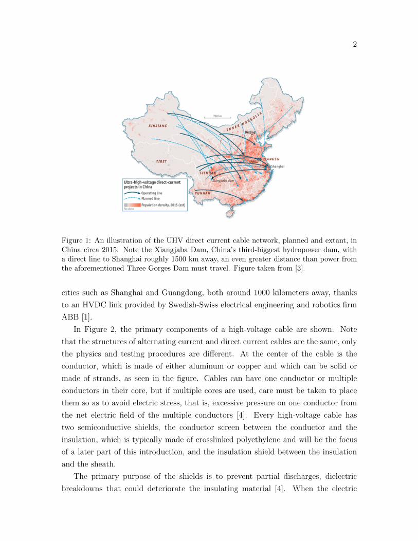
Figure 1: An illustration of the UHV direct current cable network, planned and extant, inChina circa 2015. Note the Xiangjaba Dam, China’s third-biggest hydropower dam, witha direct line to Shanghai roughly 1500 km away, an even greater distance than power fromthe aforementioned Three Gorges Dam must travel. Figure taken from [3].
cities such as Shanghai and Guangdong, both around 1000 kilometers away, thanks
to an HVDC link provided by Swedish-Swiss electrical engineering and robotics firm
ABB [1].
In Figure 2, the primary components of a high-voltage cable are shown. Note
that the structures of alternating current and direct current cables are the same, only
the physics and testing procedures are different. At the center of the cable is the
conductor, which is made of either aluminum or copper and which can be solid or
made of strands, as seen in the figure. Cables can have one conductor or multiple
conductors in their core, but if multiple cores are used, care must be taken to place
them so as to avoid electric stress, that is, excessive pressure on one conductor from
the net electric field of the multiple conductors [4]. Every high-voltage cable has
two semiconductive shields, the conductor screen between the conductor and the
insulation, which is typically made of crosslinked polyethylene and will be the focus
of a later part of this introduction, and the insulation shield between the insulation
and the sheath.
The primary purpose of the shields is to prevent partial discharges, dielectric
breakdowns that could deteriorate the insulating material [4]. When the electric

3
Figure 2: A diagram of the co-axial structure of a power cable. The principal componentsare, from A to F, the conductor, the conductor screen, the insulation, the insulation shield,the metal sheath, and the oversheath. Figure adapted from [1].
field strength around a conductor is not high enough for an electric breakdown but
still high enough to form a conductive region around a conductor, the system is
susceptible to corona discharges, which lead to economically significant power losses
[5]. The semiconductive shields ameliorate this by reducing the potential gradient
over the surface of the conductors and inside the metal sheath, regulating the electric
field around the insulation [4]. Carbon black (CB) is a necessary ingredient in these
shields for achieving appropriate conduction, so CB-filled ethylene copolymers, such
as ethylene vinyl acetate and ethylene ethyl acrylate are common choices for shielding
materials [4].
One or more sheaths form the exterior of a high-voltage cable. The inner sheath
that forms a contact with the insulation, often made of lead, copper, aluminum, or
combinations of two or three of those, serves as a grounded layer and will conduct
leakage currents [2]. Depending on the cable, the sheath in contact with the insulation
may also act as a moisture barrier, important for the many cables used underground
and underwater. An exterior sheath, such as the one seen in Figure 2, may be used as
additional protection for the inner workings of the cable against various environmental
hazards. Polyvinyl chloride (PVC) has historically been used for the outer jacket, but
the 21st century has seen the rise of halogen-free, low-fire-hazard compounds such as
ethylene vinyl acetate with aluminum trihydrate and other additives.

4
1.2 The Rise of Polymers as Insulating Materials
No component of high-voltage cables has gone through as many notable changes
or is as germane to the work presented here as the insulating component. Before
the modern era of polymer insulation began in the early 1960s, underground power
cables were insulated with oil and paper that ran through a steel pipe or an aluminum
sheath similar to the outer jackets used in modern cables. The oil had to be kept
under pressure to avoid the formation of voids that could lead to partial discharges
[2]. While this kind of insulation is still in use the world over, Figure 3 illustrates the
superiority of polymer-based insulation and the room available for future improvement
after catching up so quickly to the paper-based design.
Figure 3: The evolution of insulating materials for high-voltage cables. Note the jump inworking voltage for polymer-based insulation in the early 1960s. This is due to the use ofcrosslinked polyethylene, which will be discussed at length in this chapter. Figure takenfrom [6].
The first polymer to be widely used for insulation was polyethylene. Polyethylene
is a polymer chain produced by the polymerization of ethylene gas, C2H4. This
polymerization can be done in a few ways, each of which lead to different properties
of the resultant polymer. Coordination polymerization uses metal chlorides or metal
oxides as catalysts, which leads to a linear structure called high-density polyethylene.
For polyethylene production, the most commonly-used catalysts are the Phillips-
type catalyst, chromium oxide deposited on silica, and the Zeigler-Natta catalysts,
which generally have two components, such as TiCl4 and Al(C2H5)2Cl [7]. When the
Phillips-type catalyst is used, the polymerization process works by introducing carbon

5
dioxide to reduce Cr(VI) to Cr(II) which become organo Cr(III) sites upon exposure
to ethylene. This initiates the polymerization process, which continues until chain
termination occurs by the addition of molecular hydrogen or until the center of activity
is transferred to another molecule via beta-hydride elimination, or the conversion of an
alkyl group bonded to the chromium center to the corresponding chromium hydride
and an alkene. The exact mechanism for the polymerization process is the subject of
active research [8] [9] [10].
When the Zeigler-Natta catalysts are used, one component serves as the initia-
tor, or precatalyst, and one serves as the activator, or cocatalyst. In the case of
polyethylene, TiCl4 is the initiator and Al(C2H5)2Cl is the activator in the most
popular configuration [8]. The activator has three main roles in polymerization: ac-
tivation, stabilization, and scavenging. Activation ionizes of the metal by removal of
the halide and replacement of the alkyl group in the transition metal, the conjugate
base stabilizes the cationic species, and any excess activator scavenges the polymer-
ization medium, which is typically made of popular solvents like toluene [8]. Even
though use of the Phillips-type catalyst does not require an activator, alkylaluminum
complexes are sometimes used to scavenge the polymerization medium [11]. Figure 4
illustrates the two aforementioned catalysts.
Figure 4: The two primary types of catalysts used for coordination polymerization of ethy-lene, the Phillips-type on the left and the titanium chloride initiator bonded to the aluminumethylchloride on the right. Note the open coordination site on the titanium, which could beused to bond an ethyl group. This figure adapted from [8].
Free-radical polymerization forms polymers by the continuous addition of free-
radical chain links, chain links that bear an unpaired electron. The three steps of any
free-radical polymerization process are initiation, the formation of radicals followed
by a reaction with a monomer to create an active center for growth, propagation, the
6
rapid addition of monomers to the growing polymer chain without a change of the
active center, and termination, the destruction of the active center, which is inevitable
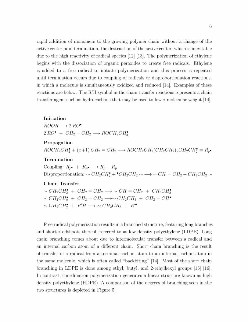
due to the high reactivity of radical species [12] [13]. The polymerization of ethylene
begins with the dissociation of organic peroxides to create free radicals. Ethylene
is added to a free radical to initiate polymerization and this process is repeated
until termination occurs due to coupling of radicals or disproportionation reactions,
in which a molecule is simultaneously oxidized and reduced [14]. Examples of these
reactions are below. The R’H symbol in the chain transfer reactions represents a chain
transfer agent such as hydrocarbons that may be used to lower molecular weight [14].
Initiation
ROOR −→ 2RO•
2RO• + CH2 = CH2 −→ ROCH2CH•2
Propagation
ROCH2CH•2 + (x+1) CH2 = CH2 −→ ROCH2CH2(CH2CH2)xCH2CH
•2 ≡ Rp•
Termination
Coupling: Rp• + Rp• −→ Rp −Rp
Disproportionation: ∼ CH2CH•2 + •CH2CH2 ∼−→∼ CH = CH2 + CH3CH2 ∼
Chain Transfer
∼ CH2CH•2 + CH2 = CH2 −→ ∼ CH = CH2 + CH3CH
•2
∼ CH2CH•2 + CH2 = CH2 −→∼ CH2CH3 + CH2 = CH•
∼ CH2CH•2 + R′H −→ ∼ CH2CH3 + R′•
Free-radical polymerization results in a branched structure, featuring long branches
and shorter offshoots thereof, referred to as low density polyethylene (LDPE). Long
chain branching comes about due to intermolecular transfer between a radical and
an internal carbon atom of a different chain. Short chain branching is the result
of transfer of a radical from a terminal carbon atom to an internal carbon atom in
the same molecule, which is often called “backbiting” [14]. Most of the short chain
branching in LDPE is done among ethyl, butyl, and 2-ethylhexyl groups [15] [16].
In contrast, coordination polymerization generates a linear structure known as high
density polyethylene (HDPE). A comparison of the degrees of branching seen in the
two structures is depicted in Figure 5.

7
Figure 5: The branching structures seen in LDPE and, scarcely, in HDPE. The branchingin LDPE is a result of free-radical polymerization and the lack of a catalyst that supervisesthe radical sites on the growing chains. As such, ethylene monomers may attach to themiddle of the chain.
The terms high density and low density are not completely accurate, as their
densities are not very different (that of HDPE ranges from 930 to 970 kg/m3 and that
of LDPE ranges from 917 to 930 kg/m3 [17]). Instead, their designations come from
their branching or lack thereof. The absence of branching in HDPE gives it a more
crystalline structure, stronger intermolecular forces, and a higher tensile strength,
while LDPE remains more flexible. As far as using polyethylene for insulation in
high-voltage cables, it is recommended that underground cables use HDPE and all
other cables use LDPE [18].
8
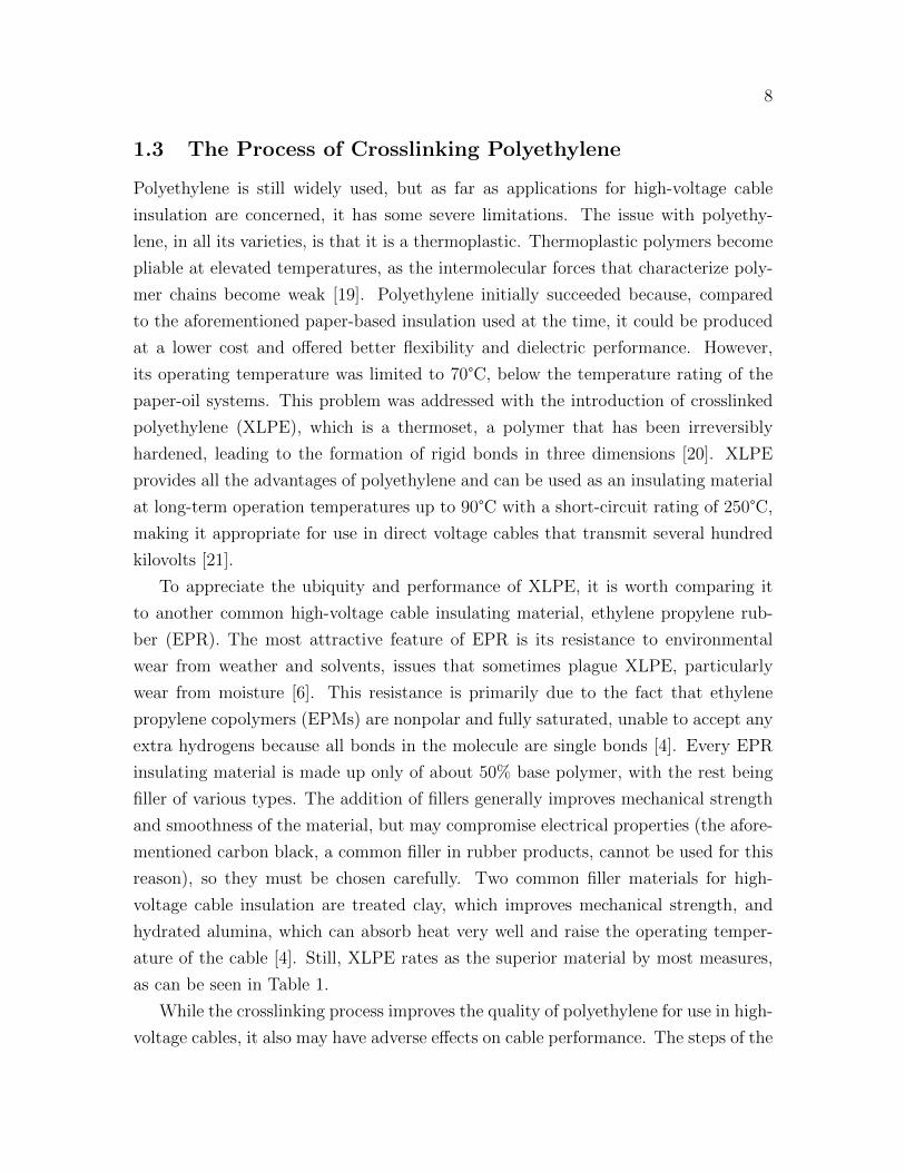
1.3 The Process of Crosslinking Polyethylene
Polyethylene is still widely used, but as far as applications for high-voltage cable
insulation are concerned, it has some severe limitations. The issue with polyethy-
lene, in all its varieties, is that it is a thermoplastic. Thermoplastic polymers become
pliable at elevated temperatures, as the intermolecular forces that characterize poly-
mer chains become weak [19]. Polyethylene initially succeeded because, compared
to the aforementioned paper-based insulation used at the time, it could be produced
at a lower cost and offered better flexibility and dielectric performance. However,
its operating temperature was limited to 70°C, below the temperature rating of the
paper-oil systems. This problem was addressed with the introduction of crosslinked
polyethylene (XLPE), which is a thermoset, a polymer that has been irreversibly
hardened, leading to the formation of rigid bonds in three dimensions [20]. XLPE
provides all the advantages of polyethylene and can be used as an insulating material
at long-term operation temperatures up to 90°C with a short-circuit rating of 250°C,
making it appropriate for use in direct voltage cables that transmit several hundred
kilovolts [21].
To appreciate the ubiquity and performance of XLPE, it is worth comparing it
to another common high-voltage cable insulating material, ethylene propylene rub-
ber (EPR). The most attractive feature of EPR is its resistance to environmental
wear from weather and solvents, issues that sometimes plague XLPE, particularly
wear from moisture [6]. This resistance is primarily due to the fact that ethylene
propylene copolymers (EPMs) are nonpolar and fully saturated, unable to accept any
extra hydrogens because all bonds in the molecule are single bonds [4]. Every EPR
insulating material is made up only of about 50% base polymer, with the rest being
filler of various types. The addition of fillers generally improves mechanical strength
and smoothness of the material, but may compromise electrical properties (the afore-
mentioned carbon black, a common filler in rubber products, cannot be used for this
reason), so they must be chosen carefully. Two common filler materials for high-
voltage cable insulation are treated clay, which improves mechanical strength, and
hydrated alumina, which can absorb heat very well and raise the operating temper-
ature of the cable [4]. Still, XLPE rates as the superior material by most measures,
as can be seen in Table 1.
While the crosslinking process improves the quality of polyethylene for use in high-
voltage cables, it also may have adverse effects on cable performance. The steps of the

9
Properties XLPE EPRDensity (g/cm3) 0.92 1.2-1.4
Tensile strength (MPa) 19 9-12Heat distortion (%) 20 5-8
Dissipation factor (%)at 20°C <0.03 0.16-0.3at 90°C <0.03 0.3-1.0
Volume resistivity (Ω-cm) at 23°C 1016 1013
Table 1: A comparison of some key properites of XLPE and EPR as insulatingmaterials for high-voltage cables. The ranges given for EPR measurements representthe range of compositions available industrially [4].
crosslinking process are similar to the steps involved in the polymerization process:
initiation, propagation, branching, and termination. The initiation step consists of
the generation of free radicals, which bond to create a dense network of polymer chains
in the propagation and branching steps until termination occurs due to the presence
of impurities or additives [22]. The branching necessary for crosslinking to occur is
more likely to happen if some kind of branching is already present, so low-density PE
is more likely to be used than the linear structure of high-density PE [23].
Initiation can be done via irradiation or via chemical reaction. In the former
method, the free radical is created when a radiation source breaks a C-H bond in
polyethylene, which in this case has a dissociation energy of 364 kJ/mol [22]. The
carbon in the free radical that has just lost its bonded hydrogen then seeks out
another hydrogen, which leads to crosslinking. Different applications require different
radiation sources and for cable insulation, the preferred source is an electron beam.
Different types of radiation produce different depths of penetration into the polymer
layer, so specific areas of the sample can be excluded from the crosslinking [24].
Penetration depth is governed by Equation 1, in which r is the rate of crosslinking, k
is a rate constant, c is the concentration of the photoinitiator, and ε is the extinction
coefficient of the photoinitiator [25].
r = k c12 e−1.151εcx (1)
While these reactions are conceptually simple and require no additives, radiation
sources are a significant monetary investment.

10
Initiation via chemical reaction comes in two varieties: organic peroxide-based
and silane-based. Peroxide crosslinking is frequently done via the Engel process, de-
veloped in the 1960s, which begins with polyethylene and the peroxide being mixed
together at low temperatures, below the peroxide decomposition temperature. Then,
the temperature is raised, and the peroxides break apart to become peroxide radi-
cals. These free radicals remove hydrogen atoms from the polymer chain, creating
more radicals. When all these radicals combine, crosslinking occurs until the supply
of peroxide is exhausted [22]. The Engel process is typically done with HDPE at
temperatures between 200 and 250°C, though LDPE could also be used at a lower
range of temperatures [26].
Extensive experimental work has been done to determine which organic perox-
ides are best suited for crosslinking of polyethylene. One of the seminal papers in
this field is the 1993 work done by Bremner and Rudin [27], comparing three dialkyl
peroxides for crosslinking with linear low-density polyethylene (LLDPE), a type of
PE produced by initiation with transition metal catalysts that has many of the prop-
erties of LDPE, but minimal branching [8][28]. Dicumyl peroxide, a popular choice
because of its favorable decomposition rate at typical crosslinking operation tem-
peratures [27], was compared to 2,5-dimethyl-2,5-di (tertiary butylperoxy)-hexane, a
common initiator for the polymerization of styrene, and 2,5-dimethyl-2,5-di (tertiary
butylperoxy)-hexyne-3. The three were evaluated according to their ability to in-
crease the storage modulus of the PE resin during curing, which is a proxy for their
crosslinking effectiveness. This work established a link between the rate of peroxide
decomposition and the rate of increase of the storage modulus of the resin during
curing and confirmed that dicumyl peroxide is effective for crosslinking polyethylene
[27].
The silane-based process begins with a silane molecule such as vinyl trimethoxysi-
lane (C5H12O3Si) grafting to a polyethylene chain [22]. For grafting to occur, a free
radical must appear somewhere on the polyethylene chain. This can be accomplished
by irradiation or in the presence of a small amount of a peroxide, usually dicumyl
peroxide. Once the polymer is Si-functionalized, it is placed in a water bath and
silicon hydroxide groups are formed by hydrolysis. Crosslinks are then formed on the
polyethylene by Si-O-Si bridges. These reactions can be accelerated by the use of a
catalyst such as dibutyltin dilaurate [22] [16]. A comparison of the three methods of
crosslinking is shown in Figure 6.

11
Figure 6: The reactions involved in each of the three crosslinking methods for polyethylene.The peroxide-based method gives the highest degree of crosslinking, up to 90%, with theirradiation-based method between 34 and 75% and the silane-based method between 45 and70%. This figure adapted from [22].
1.4 The Complications of Crosslinking Polyethylene
The primary drawback of XLPE is the formation of byproducts during the crosslinking
process that can compromise its electrical properties. Most studies have observed the
formation of acetophenone, cumyl alcohol, and methyl styrene, with at least one study
observing the formation of 2,4-diphenyl-4-methyl-1-pentene [29]. The steps involved
in crosslinking polyethylene with dicumyl peroxide have been described in detail and
Figure 7 illustrates those reactions, along with the secondary reactions that produce
the aforementioned byproducts. It can be seen in Figure 7 that acetophenone is
produced by the beta scission that breaks a methyl group off of the free radical,
cumyl alcohol is produced when the free radical interacts with the polyethylene, and
methyl styrene is produced upon the dehydration of cumyl alcohol.
The presence of these byproducts is known to lead to space charge accumulation,
in which excess electric charge creeps into the dielectric and distorts the electric
field. This can only happen in dielectrics, including vacuum, because in a conductive
material, the charge would be rapidly neutralized. The two types of space charge
accumulation are hetero charge, in which the polarity of the excess charge is opposite
that of the neighboring electrode, and homo charge, in which the inverse situation is
true [30]. Hetero charge near an electrode has been shown to be destructive in high-
voltage applications- it stresses the insulation around the electrode area by a factor of

12
Figure 7: Reaction map for the crosslinking of polyethylene illustrating how acetophenone,cumyl alcohol, methyl styrene, and methane are formed. This figure adapted from [29].
two over what would occur in the absence of excess charge and lowers the breakdown
voltage of the polymer (homo charge would increase it), making an insulating material
more susceptible to conductivity [30] [31].
In a semiconducting or insulating medium, the current is dominated by charge-
carriers injected through the electrodes and not the charge-carriers present in ohmic
materials like metals. As such, space charge current can be described by the Mott-
Gurney law (Equation 2), in which J is the current density, ε is the permittivity
of the solid, µ is the charge-carrier mobility, Va is the applied voltage and L is the
thickness of the sample. While the Mott-Gurney law is conceptually advantageous
because the only unknown is the charge-carrier mobility, it rests on many assumptions
that may not be valid for all applications [32] [33]. The most relevant to crosslinked
polyethylene is the assumption that the current cannot be limited by energetic traps,
but a few studies have proposed that the structures of acetophenone and methyl
styrene, namely the benzene ring and double bond present in both, present energetic
traps, making the Mott-Gurney law a less-than-ideal description [34] [35]. Since
13
acetophenone is the primary subject of the work presented in this document, this
idea will be revisited.
J =9
8εµV 2a
L3(2)
In early studies of space charge accumulation, effects on XLPE were separated
into four categories: the crosslinked polymer, a non-crosslinked reference, which is
essentially the base polymer, additives such as antioxidants, and residual byprod-
ucts [35] [36]. To examine charge buildup in each of these sections, charge carriers
were inserted into the XLPE sample via two electrodes and were allowed to diffuse
throughout the body of the polymer. After some time, spatial charge density profiles
were examined for evidence of a buildup of charges of the same sign (homo charge) or
charges of the opposite sign (hetero charge) around the cathode and anode. According
to charge density measurements, the non-crosslinked part shows some development
of heterocharge, which would be at odds with the theory that hetero charge is in-
troduced by the byproducts of crosslinking, but homo charge mostly takes over in
the high-voltage regime. These same results support the idea that the formation of
heterocharge is discouraged by the presence of the antioxidant and encouraged by
the presence of byproducts, which the authors of that study posit is due to the low
molecular weight of the products, which leads to them being more easily charged and
more likely to drift towards the counter electrode under DC stress [36].
The issue of space charge accumulation can be addressed by degassing, the re-
moval of dissolved gases, often via heating. Degassing should be done to eliminate
the flammable methane byproduct and it has been shown that the removal of gasses
can relieve some pressure on the cable insulation that might build up when an exter-
nal sheath is in place, as is often the case for high-voltage cables [21]. This pressure
relief in turn increases the stress necessary for space charge to begin leaking into the
insulating material [35]. Still, even though the operating threshold of the cable might
be improved by degassing, care must be taken to ensure that the insulating perfor-
mance of the material is not seriously compromised by the presence of crosslinking
byproducts.

14
1.5 A Survey of Experimental and Computational Studies
The last section of this introductory chapter is a lead-in to the methodology chapter of
this document, as it gives a brief overview of previous experimental and computational
studies that pertain to most of the concepts and phenomena described in this section.
An important experimental task is to be able to distinguish between different
grades of polyethylene using spectroscopy. It has been shown that Fourier-Transform
Infrared (FTIR) spectroscopy, in which a beam containing several frequencies of light
is shone on a sample, the degree to which the beam is absorbed by that sample is
measured by the displacement of a mirror, and those displacement measurements are
transferred back to the frequency domain, is an appropriate tool for this. Differ-
ent varieties of PE all show the same peaks in a spectrograph, but the degrees of
branching that differentiate them are reflected in the relative intensities of the peaks
[37]. The FTIR peaks of polyethylene are shown in Table 2. The ability of FTIR to
detect such subtleties has also proved useful in analyzing possible byproducts of the
crosslinking process. One study found that the universally utilized dicumyl peroxide
caused partial oxidation of the polymer, which the authors posited could be stopped
by the introduction of the antioxidant Irganox 1081 [38].
Band (cm−1) Assignment2919 CH2 Asymmetric Stretching2851 CH2 Symmetric Stretching
1473 and 1463 Bending Deformation1377 CH3 Symmetric Deformation
1366 and 1351 Wagging Deformation1306 Twisting Deformation1176 Wagging Deformation
731-720 Rocking Deformation
Table 2: The primary absorptions of polyethylene in the IR region and what theycorrespond to [37].
FTIR has been of use in studying the aging and degradation of polyethylene in
high-voltage cables. For this, FTIR can be enhanced by a pairing with attenuated
total reflectance (ATR) sampling, which allows samples to be studied in the liquid
or solid state without any preparation by use of a crystal in contact with the sample
that absorbs the beam from the spectrometer and forms an evanescent wave that
passes into the sample [39]. FTIR can monitor the polymer over time and is capa-
ble of detecting degradation byproducts, mainly ketones, esters, and lactones [40].

15
Similar observations can be made using magic angle spinning hydrogen-based nu-
clear magnetic resonance, or H-MAS NMR, in which the sample is rotated at the
resolution-improving “magic angle” of 57.74 degrees relative to the external magnetic
field generated by a hydrogen nucleus. Perturbations of the nuclear spins of the
sample correspond to radio frequencies, which can be assembled to form a spectrum
[41] [42]. H-MAS NMR studies have been able to detect the aforementioned aging
products, as well as significant quantities of aldehydes [43].
Extensive computational work has been done on all aspects of crosslinked polyethy-
lene. One such study looked at the possibility of using gold atoms in the crosslinking
process, creating carbon-gold-carbon bridges to serve as the backbone of the polymer.
The use of metal atoms leads to dispersion interactions during crosslinking, which were
modeled with density-functional theory (DFT), one of the key methods used in the
work presented in this document. The DFT energetics revealed reasonable binding
energies [44]. Another study imitated the methods of the FTIR- and NMR-based
works by monitoring microstructural changes that occur during crosslinking with a
Monte Carlo simulation. The extensive branching of polyethylene used for crosslink-
ing makes it a good target for the probabilistic nature of Monte Carlo simulations [45].
The use of Monte Carlo has been used to generate branched and crosslinked struc-
tures, which are then subject to DFT energetics calculations to obtain an accurate
picture of electronic states of polyethylene [46].
Electronic states were of interest to a few studies that used molecular dynamics
(MD) to investigate the presence of energy traps in polyethylene, with one study
asserting the acetophenone byproduct as an energy trap based on its influence on
the density of states and another looking at electron affinity in an environment with
various chemical defects [47][48]. MD has also been used to analyze the strain asso-
ciated with crosslinking and scission reactions in several different polymers [49] [50].
Possibilities for improving the crosslinking of polyethylene have been studied with
DFT, optimizing the bond lengths and calculating the energies associated with graft-
ing voltage stabilizers to the polymer chain [51]. The methods used in the original
research presented in this document draw inspiration from all the aforementioned
studies and will be discussed in the next chapter.

16
2 METHODS
How This Work Was Done
This second section serves to explain the methodology used for the research pre-
sented in this work. This section begins by discussing the key equations of density-
functional theory (DFT) and the improvements made by the development of con-
strained density- functional theory (cDFT), then will describe the process of conver-
gence testing necessary to find the right basis set and exchange-correlation functionals,
in order to have an appropriate level of approximation in the DFT calculations. Fol-
lowing this, the process for calculating an equilibrium mixture of electronic states at
finite temperatures based on DFT energetics will be detailed. These steps will all be
repeated for the reactive force field calculations done by the author. These points will
all be addressed according to their relevance to the introduction and results sections
of this work.
2.1 The Essentials of Density Functional Theory
The starting point for the development of density-functional theory (DFT) is the
assertion that the fundamental properties of materials can be determined and pre-
dicted solely on the basis of quantum mechanical considerations, without knowing
any empirical material properties such as specific heat capacity or tensile strength.
To start solving these kinds of problems, one could consider the many-electron time-
independent Schrodinger equation (Equation 3), in which H is the Hamiltonian op-
erator of the many-body system, Ψ is the wavefunction of the system, and E is the
total energy of the system.
H |Ψ〉 = E |Ψ〉 (3)
The central problem associated with this kind of calculation is that it quickly becomes
prohibitively complex. This becomes clear when looking at a more complete version
of the Schrodinger equation, seen in Equation 4, in which m is the electron mass and
the three terms in brackets are, from left to right, the kinetic energy of each electron,
the electrostatic interaction energy between each electron and all the nuclei, and the
electrostatic interaction energy between different electrons [52].[− h2
2m
N∑i=1
∇2i +
N∑i=1
V (ri) +N∑i=1
∑j<1
U(ri, rj)
]|Ψ〉 = E |Ψ〉 (4)
17
For a concrete example, consider the benzene ring featured in the acetophenone
molecule, which has 12 nuclei and 42 electrons. In three dimensions, this would lead
to a wavefunction with (3 x 12) + (3 x 42) = 162 variables. It is known that the
computational complexity necessary to solve an eigenvalue problem increases faster
than the square of the number of coordinates and often at a cubic rate [53]. So, the
best-case scenario for this calculation is that it would require 1622 = 2 × 10⁴ steps.
The number of steps can be reduced to some extent with the Born-Oppenheimer
approximation, which accounts for the substantial differences in mass and time scales
of motion of the electrons and the nuclei by expressing the wavefunction for the
system as the product of an electronic and a nuclear wavefunction, eliminating cross-
terms in the Hamiltonian [54]. This breaks the calculation down into two steps, first
a calculation with the 126 electronic variables (104 steps), then a calculation that
applies this result to each of the 36 nuclear variables (103 steps). This is a marked
improvement, but is still computationally impractical.
Another inconvenience is that wavefunctions cannot be observed directly. Thank-
fully, it is possible to measure the probability that the N electrons in the system are at
particular coordinates. This is further simplified by the fact that it not important to
distinguish between individual electrons, so the quantity of interest is the probability
that a set of N electrons in any order have the coordinates r1. . . rN . The physical
quantity that matches this description well is the electron density as a function of po-
sition, n(r) [52]. Equation 5 shows the electron density in terms of individual electron
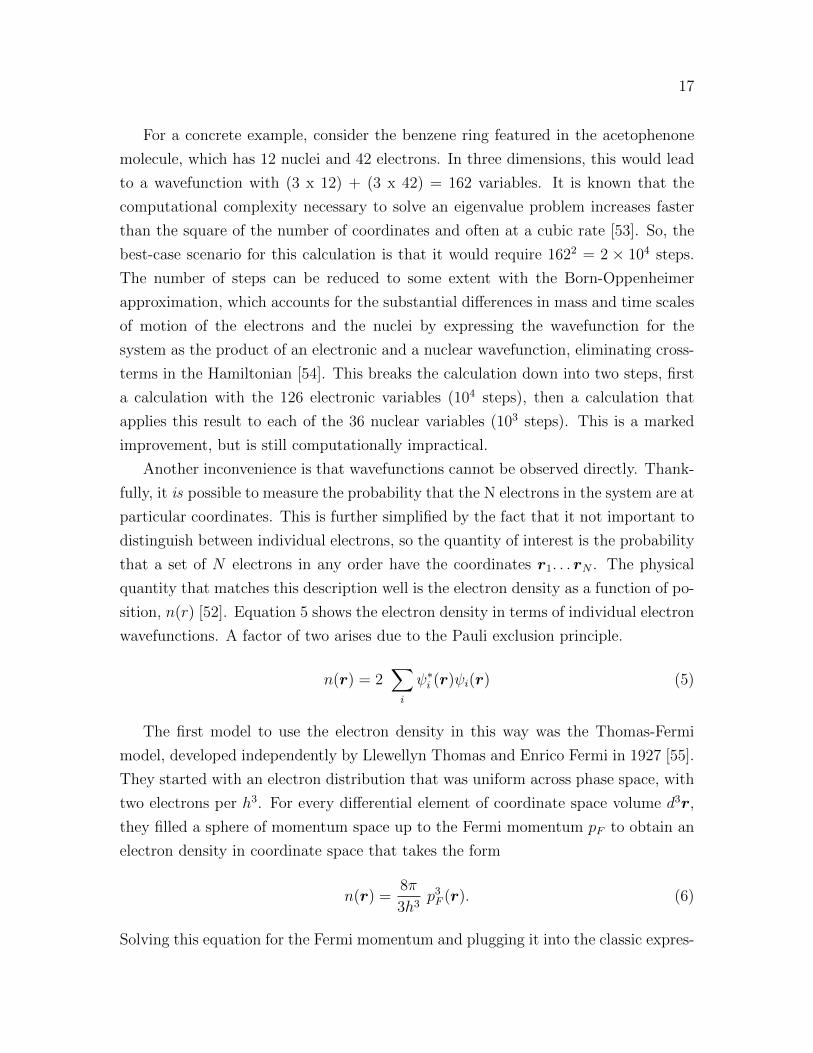
wavefunctions. A factor of two arises due to the Pauli exclusion principle.
n(r) = 2∑i
ψ∗i (r)ψi(r) (5)
The first model to use the electron density in this way was the Thomas-Fermi
model, developed independently by Llewellyn Thomas and Enrico Fermi in 1927 [55].
They started with an electron distribution that was uniform across phase space, with
two electrons per h3. For every differential element of coordinate space volume d3r,
they filled a sphere of momentum space up to the Fermi momentum pF to obtain an
electron density in coordinate space that takes the form
n(r) =8π
3h3p3F (r). (6)
Solving this equation for the Fermi momentum and plugging it into the classic expres-

18
sion for kinetic energy, K = 12mv2, leads to kinetic energy as a functional (function
of a function) of the electron density, seen below in Equation 7 [55].
K[n] =3h2
10me
(3
8π
) 23∫n
53 (r) d3r (7)
This equation was combined with classical expressions of electron-nuclear and electron-
interactions to obtain a total energy. However, this kinetic energy functional was only
a rough approximation and density-functional theory did not stand on firm ground
until the work of Walter Kohn and Pierre Hohenberg in the 1960s.
Kohn and Hohenberg were able to lay the foundation for DFT with their proofs of
two fundamental theorems [56]. The first says that the ground-state energy obtained
from the Schrodinger equation is a unique functional of the electron density, which is
equivalent to saying that the ground-state electron density determines all properties
of the ground state. This is important because it reduces the problem of solving
the Schrodinger equation (i.e. finding the ground state energy) from a problem with
potentially thousands of variables to a problem with three variables. The second
theorem gives some more information about the functional, stating that the electron
density that minimizes the overall functional is the true electron density corresponding
to the full solution of the Schrodinger equation. This leads to what is called the
variational principle, the idea that if the true form of the functional were known,
the electron density could be varied until the energy is minimized and the electron
density could be determined in this way [57].
The functional described by the Hohenberg-Kohn theorems can be written in
terms of the single-electron wavefunctions ψi(r) seen in Equation 8 which, again,
define the electron density. This energy functional can be written as
E[ψi] = Eknown[ψi] + EXC [ψi] (8)
in which the “known” terms are those that can be written down in a simple ana-
lytical form and the exchange-correlation (XC) terms are everything else (exchange
correlation functionals will be discussed in detail later in this chapter). The known
terms can be seen below in Equation 9 and are, from left to right, the electron kinetic
energies, the Coulomb interactions between electrons and the nuclei, the Coulomb
interaction between pairs of electrons, and the Coulomb interaction between pairs of

19
nuclei [52].
Eknown[ψi] = −h2
m
∑i
∫ψ∗i∇2ψid
3r +
∫V (r)n(r)d3r
+e2
2
∫ ∫n(r)n(r′)
|r − r′|+ Eion (9)
Even with these terms and a reasonable description of the exchange-correlation
terms, the act of solving the Schrodinger equation is not made any easier. Kohn and
Sham addressed this, showing that the correct electron density could be found by
solving a system of equations in which each equation only involves a single electron
[58]. These Kohn-Sham equations take the form[− h2
2m∇2 + V (r) + VH(r) + VXC(r)
]ψi(r) = εiψi(r). (10)
This is very similar to the Schrodinger equation, except there are no summations
because the solutions of the Kohn-Sham equations are single-electron wavefunctions
that only depend on the three spatial variables. The first of the three potentials, V in
Equation 10 is the same potential as in the full Schrodinger equation and defines the
interaction between an electron and the nuclei surrounding it. The second potential,
VH is called the Hartree potential and is expressed as
VH(r) = e2
∫n(r)′
|r − r′|d3r′. (11)
This potential describes the Coulomb interaction between the electron featured in
a single Kohn-Sham equation and all other electrons in the system. The Hartree
potential includes some degree of self-interaction, since every individual electron being
considered is also one of the electrons in the system. The correction for this self-
interaction is included in the third potential, VXC , which defines the contribution
of exchange interactions, interactions that occur between indistinguishable particles,
and correlation interactions, the influence of all electrons on the movement of one
electron, to single-electron equations. VXC is defined as the functional derivative
(conceptually very similar to a regular derivative) of the exchange-correlation energy:
VXC(r) =δEXC(r)
δn(r). (12)

20
The steps involved in these calculations form a cycle. To solve the Kohn-Sham
equations, the Hartree potential must be defined and to define the Hartree potential,
the electron density must be known. But knowing the electron density requires know-
ing the single-electron wavefunctions, which are obtained by solving the Kohn-Sham
equations. Sholl and Steckel’s seminal DFT book describes the steps necessary for
calculations in the self-consistent cycle [52]:
1. Define a trial electron density n(r)
2. Solve the Kohn-Sham equations using the trial electron density to find the
single-electron wavefunctions, ψi(r)
3. Calculate the electron density defined by the Kohn-Sham single-particle wave-
functions
4. Compare the calculated electron density with the electron density used to solve
the Kohn-Sham equations. If they are the same, then this is the ground-state
electron density that can be used to calculate the total energy. If not, the trial
electron density must be changed in some way and this process starts again at
Step 2.
The next section of this chapter explains how to apply this self-consistent procedure
to the acetophenone system that is the focus of this thesis.

21
2.2 Constrained Density Functional Theory
Since the advent of DFT, many methods have been developed to improve and build
upon it. One of the most versatile is constrained density functional theory (CDFT)
[59]. One CDFT formalism was laid out by Dederichs et al in the 1980s [60], with
the idea of finding the electronic ground state of a system subject to the constraint
that there are N electrons in a volume Ω. This was achieved by adding a Lagrange
multiplier to the familiar DFT energy functional form:
E(N) = E[n] + λ
(∫Ω
n(r) d3r −N)
(13)
The addition of this Lagrange multiplier was enough to ensure that this calculation
would yield the lowest-energy state that contained exactly N electrons in a volume Ω.
This tuning of the functional also helps mitigate the aforementioned self-interaction
error that plagues many DFT functionals [59].
Figure 8: The acetophenone molecule, adapted from [61].
This formalism is the basis for much of the work presented in this thesis. The
previously-discussed acetophenone molecule that forms as a byproduct in peroxide-
based polyethylene crosslinking reactions is the species of interest here. Since it
is well established that the presence of byproducts compromises the integrity of the
cable, it is worth investigating how acetophenone behaves when exposed to free charge
carriers. As such, CDFT has been used to study the acetophenone radical anion, with
the electron being constrained to each of the 17 atoms in the molecule (seen above
in Figure 15). The DFT energies of each of these constrained states were compared

22
to each other to determine the locations on the molecule most likely to attract the
excess electron. This allows inferences to be drawn about possible chemical reactions
involving the acetophenone radical anion. The next several sections of this chapter
describe the details of these energy calculations.
2.3 Choosing a Basis Set
The first step in these calculations is selecting an appropriate basis set, the set of
functions used to represent the electronic wavefunction. The basis sets considered
for the work presented here include Pople basis sets [62] and correlation-consistent
basis sets [63]. Pople basis sets are described as “split-valence” basis sets because
they represent valence orbitals, which contain the valence electrons that primarily
participate in bonding, with multiple basis functions. These basis sets are of the
form X-YZG, in which X represents the number of primitive Gaussians (G being
Gaussian) making up each core orbital basis functions, and the Y and Z indicate that
the valence orbitals are made of two basis functions each, one a linear combination of
Y primitive Gaussians and the other a linear combination of Z primitive Gaussians.
If the valence orbitals are described by three basis functions, the basis set may take
the form X-YZWG.
Additionally, polarization functions (denoted by * or ** if polarization functions
are on hydrogen and heavy atoms) may be added to describe the polarization of the
electron density of a particular atom and diffuse functions (denoted by + or ++ if
diffuse functions are on hydrogen and heavy atoms) may be added to better describe
the “tail” of the orbital function, far away from the nucleus.
The correlation-consistent basis sets were designed for converging Post-Hartree-
Fock calculations, calculations that describe correlation between electrons instead of
simply repulsion. They are typically written as cc-pVNZ, in which cc-p stands for
correlation-consistent polarized, V indicates that they are valence-only, and NZ indi-
cates the number of basis functions that make up each orbital (D=double, T=triple,
etc.). Z stands for “zeta,” which was commonly used as an exponent on early ba-
sis functions [64]. The basis sets considered for this work were 6-31G, 6-31G**,
6-311G**, and cc-pVDZ. No basis sets with diffuse functions were considered as it
is known that CDFT calculations sometimes have issues with diffuse functions (this
will be discussed further in the CDFT results section) [59].
These basis sets were evaluated with a sort of convergence test, seeing how close

23
they could get to the electron affinity (EA) and ionization potential (IP) predictions
of a much larger basis set, aug-cc-pVDZ (augmented with diffuse functions). Note
that these EA and IP values were not obtained by CDFT calculations, but by adding
whole charges to the neutral acetophenone molecule and finding the energy difference
between the -1 charge and neutral states (EA) and the between the +1 charge and
neutral states (IP). The results are shown in Tables 3 and 4 for three select functionals
that will be discussed in the following section, B3LYP, PBE0, and pure HF. Based
on this convergence test, the 6-311G** basis set was chosen.
Basis set B3LYP PBE0 Pure HF6-31G 9.0445 9.1318 7.806
6-31G** 8.9493 9.0295 7.81126-311G** 9.0465 9.1925 7.9178cc-pvdz 9.06 9.1209 7.886
aug-cc-pvdz 9.1777 9.1885 9.1127
Table 3: Values of the ionization potential for different basis sets
Basis set B3LYP PBE0 Pure HF6-31G 0.1542 0.1167 0.7658
6-31G** 0.2818 0.2402 1.03586-311G** -0.0344 -0.0261 0.8492cc-pvdz 0.0922 0.0721 0.9097
aug-cc-pvdz -0.3526 -0.3053 0.7017
Table 4: Values of the electron affinity for different basis sets

24
2.4 Tuning the Hybrid Functionals
The next step in establishing an appropriate level of theory for these calculations is
finding an acceptable exchange-correlation functional. The functionals considered for
this work improve upon Hartree-Fock (HF) exact exchange functionals by hybridizing
them with energy functionals from other sources, which is known to improve predic-
tions of many molecular properties [65]. These other energy functionals depend on
two approximations commonly employed in DFT calculations: the local density ap-
proximation (LDA) and the generalized gradient approximation (GGA).
The LDA formalism is based on the treatment of electrons in the homogeneous
electron gas and an LDA functional depends only on the density at the point in
space where the functional is being evaluated. The LDA scheme assumes that elec-
tron density is uniform, which leads to underestimating the exchange energy and
overestimating the correlation energy [66]. These errors compensate for each other
to a degree, but an improvement over LDA is the GGA scheme, in which the non-
homogeneity of the electron density is captured by writing a functional in terms of
the electron density gradient [67].
The first hybrid functional considered was B3LYP, the constituent parts of which
are seen below in Equation 14, in which EGGAx is a GGA approximation of the Becke 88
exchange functional, EGGAc is a GGA approximation of the Lee, Yang, Parr functional,
and ELDAc is the VWN LDA approximation of the correlation functional [68].
EB3LY Pxc = ELDA
x + 0.20(EHFx − ELDA
x ) + 0.72(EGGAx − ELDA
x )
+ ELDAc + 0.81(EGGA
c − ELDAc ) (14)
The three parameters that give B3LYP its name are borrowed from parameterization
done by Becke [69]. The other hybrid functional considered for this work was PBE0,
which breaks down as seen in Equation 15.
EPBE0xc =
1
4EHFx +
3
4EPBEx + EPBE
c , (15)
where EHFx is the Hartree-Fock exact exchange functional, EPBE
x is the PBE exchange
functional, and EPBEc is the PBE correlation exchange functional [70].
The parameter that needed tuning was the percentage of Hartree-Fock exact ex-
change, which avoids the self-interaction error that results from functionals with a
correlation component and leads to problems such as overestimated electron affini-

25
ties [71]. A range of HF contributions above the base percentages seen in Equations
14 and 15 were evaluated on the basis of compliance with a DFT-adapted version of
Koopmans’ theorem, which states that the negative of the energy of the highest occu-
pied molecular orbital (HOMO) should equal the ionization potential of the molecule
and the negative of the energy of the lowest unoccupied molecular (LUMO) orbital
should be equal to or slightly less than the electron affinity [72]. It can be seen in
Figure 9 that, for both functionals, this condition is met at an HF contribution of
about 65%. Changing the HF contribution means changing how much other terms
contribute to the exact exchange. For the PBE0 functional, this means that the PBE
exchange contribution is only 35% and for the B3LYP functional, since there are three
contributions to the exchange, the Becke 88 local contribution is dropped to 35% and
the Becke 88 nonlocal weight is dropped from 0.72 to 0.315.
Figure 9: Determining the best Hartree-Fock percentage for the hybrid functional by lookingfor Koopmans’ compliance. Figures A and B are the B3LYP hybrid functional and FiguresC and D are for PBE0.

26
2.5 Calculating an Equilibrium Mixture
With all the parameters for the CDFT calculations established, a mixture composition
of electronic states can be obtained. As is generally recommended, the charge and
spin are constrained in each calculation. A charge of -1, representing the electron of
the acetophenone radical anion, and a spin of 1, making this extra electron an alpha
electron, are constrained to each of the 17 atoms that make up acetophenone. A DFT
energy is obtained from each calculation, which was done with the NWChem software
[73]. The difference between this energy and the energy of the “ground state” of an
electron constrained to the entirety of the molecule is calculated and then a baseline
equal to the resulting lowest energy is subtracted, leaving one state at zero energy.
These relative energies are treated as ∆G values and the equation below, taken
from a 1997 paper by van Duin et al [74], is used to calculate the percentage of each
of the 17 states in the equilibrium mixture. Entropic effects are ignored. A mixture
is then calculated for a range of temperatures: 300, 400, 500, 600, 700, 800, 900, and
1000 K.
%Ci = 100 ×exp(
∆Gi−∆G1
RT
)1 +
ns∑n=2
exp(
∆Gn−∆G1
RT
) (16)

27
2.6 Atomic Orbital-Based Population Schemes
This thesis compared the equilibrium mixture composition obtained from CDFT en-
ergies with population analysis schemes that estimate how partial charges distribute
themselves among the atoms of a molecule. Two of the most prominent are the Mul-
liken and Lowdin schemes. The Mulliken scheme is simpler in terms of the underlying
mathematics, if less robust. In the Mulliken scheme [75], if the coefficients for the ba-
sis functions of the atomic orbitals are written as Cµi for basis function µ in molecular
orbital i, then the terms of a charge density matrix can be described as a probability
density and written as
Dµν = 2∑i
CµiC∗νi (17)
for a closed shell system in which each orbital is doubly occupied, hence the factor
of two. The matrix Sµν describes the overlap between the atomic orbitals that make
up the molecular orbitals and the product of Sµν and the density matrix Dµν is the
population matrix
Pµν = DµνSµν . (18)
The sum of all the Pµν terms over all basis functions µ is called the Gross Orbital
Product (GOP) for the atomic orbital ν. The sum of the GOPs of each orbital should
be the total number of electrons. When we sum the GOPs of all orbitals ν associated
with a given atom A, we obtain a quantity known as the Gross Atom Population
(GAP). The Mulliken charge, Q, on that atom A is then the difference between the
charge of a free atom, Z, and the GAP, expressed as
QA = ZA −GAPA. (19)
While the Mulliken population scheme is easy to understand and implement, it
suffers from an explicit dependence on the basis set. If the complete basis set for a
molecule can be spanned by placing functions on a single atom, the Mulliken scheme
will assign every electron in the system to that single atom, which is clearly unphysical
and will yield inconsistent results.
An alternative to the Mulliken scheme that reduces the basis set dependence
while not deviating too far in terms of the underlying theory is the Lowdin pop-
ulation scheme. While the Mulliken scheme does not require anything of its basis
functions, the Lowdin scheme transforms all the atomic orbitals to an orthogonal ba-

28
sis with a symmetric orthogonalization scheme that gives all the wavefunctions equal
weight in calculating linear combinations of wavefunctions to obtain the new basis
set. The transformation found by Lowdin in his seminal 1950 paper [76] to produce
an orthonormal basis set closest to the original basis is the linear transformation
S12 , where S is the overlap matrix. To examine the validity of this transformation
within the established mathematical framework, it is necessary to return to Equation
18. When the aforementioned transformation is applied, the product defining the
population matrix becomes
Pµν = (S12PS
12 )µν . (20)
The following is a well-known property of square matrices: tr(ABC) = tr(BCA) =
tr(CAB). This means that, for any value of λ, the trace of SλPSλ−1 will give the
same total number of electrons, but will give different partial traces for the different
atoms, leading to potential differences in delocalization [77].
While atomic-orbital based population schemes can be unreliable when used in
conjunction with CDFT [59], no issues were found when performing a population
analysis of the “ground state” of the acetophenone anion, that is, the state in which
the free electron is “constrained” to the entire molecule and allowed to delocalize. The
Mulliken scheme was chosen over the Lowdin scheme due to easier convergence of the
CDFT energy calculations. None of the issues with the Mulliken scheme presented
themselves in this work.

29
2.7 The Essentials of Reactive Force Field Calculations
At the turn of the 21st century, established quantum chemistry methods allowed
calculation of the geometry and energy of small molecules, but fell short when it
came to predicting the dynamics of larger molecules [78]. The addition of force fields
grants the ability to accurately describe dynamical properties, but most force fields
could not describe chemical reactivity. The exception was the Brenner potential,
which could describe bond breaking, but did not include van der Waals and Coulomb
interactions [79]. A few bond-order-based methods emerged that improved on this,
but did not fully address the need to be able to fully describe bond formation, bond
breaking, and equilibrium geometries [80] [81].
This void was filled by the development of the ReaxFF method. This reactive
force field method divides the energy of the system into several contributions, each
seen in Equation 21.
Esystem = Ebond + Ecoord + Eval + Etors
+ EvdWaals + ECoulomb + Especific (21)
The bond energy can be calculated from the bond order. In turn, one of the as-
sumptions central to ReaxFF is that the bond order can be calculated directly from
interatomic distances according to the following equation:
BOij = exp
[pbo,1 ·
(rσijr0
)pbo,2]+ exp
[pbo,3 ·
(rπijr0
)pbo,4]+ exp
[pbo,5 ·
(rππijr0
)pbo,6](22)
in which BO is the bond order between atoms i and j, rij is the distance between
atoms i and j, the r0 terms are equilibrium bond lengths, and the pbo terms are
empirically derived. The superscripts σ, π, and ππ refer to sigma bonds, pi bonds,
and second pi bonds [82].
Atom type r0,σ(A) r0,π(A) r0,ππ(A) pover(kcal/mol) punder(kcal/mol)C 1.399 1.266 1.236 52.2 29.4H 0.656 - - 117.5 -
Table 5: Atom parameters used in Equations 22, 24, and 25 [78].

30
This equation is continuous, ensuring continuity across transitions between σ,
π, and ππ bonds. This yields the differentiable potential energy surface necessary
for force field calculations. This equation also accounts for long-distance covalent
interactions in transition state structures, which allows the force field to predict re-
action barriers. This covalent range is typically taken to be 5 angstroms, but can
be expanded if elements with large covalent radii are involved. One danger with this
approach is the inclusion of false bonded character between neighboring, non-bonded
species such as the hydrogens in a methane molecule. To combat this, a correction is
typically added to the bond order [82]. This corrected bond order is used to calculate
bond energy, as seen in Equation 23, in which all the variables are the same as those
used in the bond order equation [78].
Ebond = −De ·BOij · exp[pbe,1
(1−BOpbe,1
ij
)](23)
Even after bond order corrections, the coordination of the molecule may not be
exactly right. For an over-coordinated atom (e.g. bond order of greater than four
for carbon or one for hydrogen), an energy penalty is assessed. In the case of under-
coordination, an energy term is added to account for the contributions from the
resonance of the π-electron between neighboring under-coordinated atoms. This res-
onance contribution and the over-coordination penalty are reflected in the Ecoord term
and the forms of their energies are seen in Equations 24 and 25, respectively.
Eover = pover ·∆i ·(
1
1 + exp(−8.90 ·∆i)
)(24)
Note: The ∆i terms in all of these equations refer to the difference between the bond
orders around an atomic center and its valency.
Eunder = −punder ·1− exp(1.94 ·∆i)
1 + exp(3.47 ·∆i)· f1(BOij,π,∆j) (25a)
f1(BOij,π,∆j) =1
1 + 5.79 · exp
(12.38 ·
neighbors∑j=1
∆j ·BOij,π
) (25b)
The valence angle contribution, captured in the Eval term, must go to zero as the
bond orders of the associated atoms go to zero. Equation 26a describes the energy
associated with deviations of the angle Θijk from the equilibrium angle Θ0. The bond-

31
Bond type De(kcal/mol) pbe,1 pbo,1 pbo,2 pbo,3 pbo,4 pbo,5 pbo,6C-C 145.2 0.318 -0.097 6.38 -0.26 9.37 -0.391 16.87C-H 183.8 -0.454 -0.013 7.65 - - - -H-H 168.4 -0.310 -0.016 5.98 - - - -
Table 6: Bond parameters used in Equations 22 and 23 [78].
order dependent term in Equation 26b ensures that the energy associated with the
valence angle goes to zero and bond dissociation occurs. Equation 26c describes the
effects of under- and over-coordination of the bond’s central atom j. These equations
capture the dependence of the equilibrium valence angle on bond order [78].
Eval = f2(BOij) · f2(BOjk) · f3(∆j) ·(ka − ka exp
[−kb(Θ0 −Θijk)
2])
(26a)
f2(BOij) = 1− exp(−1.49 ·BO1.28
ij
)(26b)
f3(∆j) =2 + exp(−6.30 ·∆j)
1 + exp(−6.30 ·∆j) + exp(pv,1 ·∆j)·[
2.72− 1.72 · 2 + exp(33.87 ·∆j)
1 + exp(−33.87 ·∆j) + exp(−pv,2 ·∆j)
] (26c)
The torsion angle, the angle between the two outer bonds of three consecutive
bonds, whose energy contributions are tied up in the Etors term, is also highly bond
order-dependent. The valence angle-dependent sine terms in Equation 27a ensure
that the torsion angle contribution goes to zero as either of the two valence angles,
Θijk or Θjkl, approaches 180 degrees. Equation 27b ensures that the torsion angle
contribution goes to zero as the bonds in the torsion angle dissociate and Equation
27c ensures that the torsion contribution will not be disproportionate if atoms j and
k are over-coordinated.
Etors = f4(BOij, BOjk, BOkl) · sin Θijk ·Θjkl[1
2V2 · exp
[pl(BOjk − 3 + f5(∆j,∆k))
2]· (1− 2 cosωijkl)
+1
2V3 · (1 + 3ωijkl)
(27a)
f4(BOij, BOjk, BOkl) = [1− exp(−3.17 ·BOij)]·
[1− exp(−3.17 ·BOjk)] · [1− exp(−3.17 ·BOkl)](27b)
f5(∆j,∆k) =2 + exp(−10.00 · (∆j + ∆k))
1 + exp(−10.00 · (∆j + ∆k)) + exp(0.90 · (∆j + ∆k))(27c)

32
Valence angle Θ0 ka(kcal/mol) kb((1/rad)2) pv,1 pv,2C-C-C 71.31 35.4 1.37 0.01 0.77C-C-H 71.56 29.65 5.29 - -H-C-H 69.94 17.37 1.00 - -C-H-C 0 28.5 6.00 - -H-H-C 0 0 6.00 - -H-H-H 0 27.9 6.00 - -
Table 7: Valence angle parameters used in Equation 26 [78].
Torsion angle V2 V3 plC-C-C-C 21.7 0.00 -2.42C-C-C-H 30.5 0.58 -2.84H-C-C-H 26.5 0.37 -2.33
Table 8: Torsion angle parameters used in Equation 27 [78].
Energies associated with noncovalent interactions, namely van der Waals and
Coulomb forces, are also incorporated into the system energy by ReaxFF for all
pairs of atoms. The van der Waals contribution, captured in the EvdWaals term, uses
a distance-corrected Morse potential, seen in Equation 28. The use of a shielded
interaction, seen in Equation 28b, avoids excessive repulsion between bonded atoms
and atoms sharing a valence angle [78].
EvdWaals = Dij ·[exp
(αij
(1− f6(rij)
rvdW
))− 2 · exp
(αij2
(1− f6(rij)
rvdW
))](28a)
f6(rij) =
[r1.69ij +
(1
λw
)1.69]0.592
(28b)
The system’s Coulomb energy uses a shielded potential to account for orbital overlap
between atoms close to each other, seen in Equation 29. The atomic charges qi and
qj are calculated using the electron equilibration method (EEM), which accounts for
geometry and connectivity in assigning atomic charges and, like DFT, is based on the
work of Hohenberg and Kohn [83].
ECoulomb = C · qi · qj(r3ij +
(1γij
)3)1/3
(29)

33
Atom type rvdW (A) α γW (A) γCoulomb(A)C 3.912 10.71 1.41 0.69H 3.649 10.06 5.36 0.37
Table 9: Coulomb and van der Waals parameters used in Equations 28 and 29 [78].
The last term in Equation 21, Especific, captures assorted dynamics that might
arise in particular systems. For example, an allene compound, in which a carbon
atom is double-bonded to each of its two adjacent carbon centers, requires an energy
penalty be assessed to capture its stability [78]. The relationships between these
energy terms and their roles in the ReaxFF calculation process is depicted in Figure
10.
Figure 10: An illustration of the ReaxFF calculation process [82].

34
2.8 Improvements in the Treatment of Electrons and Holes
Electrons are treated implicitly in the ReaxFF formulation, that is, only their wave-
like behavior is captured. The lack of an explicit electron description makes it im-
possible to accurately calculate electron affinities and ionization potentials, making
ReaxFF unsuitable for describing redox chemistry [84]. The eReaxFF method intro-
duces an explicit, or particle-like, electron description into the ReaxFF framework. In
eReaxFF, the electron or hole is treated as a particle that carries a -1 or +1 charge,
respectively. Nuclei are treated as point charges and charge carriers have Gaussian
wavefunctions of the form Ψ = exp(−α(r − r′)2). The electrostatic interaction be-
tween the charge carriers and the nuclei is written as
Eelec =1
4πε0β∑i,j
ZiRij
erf(√
2αRij) (30)
in which Zi is the nuclear charge, Rij is the distance between the electron and nucleus,
and α and β are constants that depend on the atom type. Interactions between
electrons are treated as Coulombic interactions between point charges.
When explicit electron/hole degrees of freedom are introduced, the valency of
and number of lone pairs on an atom must be subject to change. In eReaxFF, an
exponential function is used to describe the number of electrons on a particular atom
to ensure that a single electron can split itself among multiple atom centers. This
function is seen in Equation 31, in which Rij is the distance between the charge carrier
and the atom center and pval is a general parameter in the force field [85].
nel = exp(−pval ·R2
ij
)(31)
As seen in Figure 10, in the ReaxFF method, bonded and non-bonded interac-
tions are calculated separately. In eReaxFF, the explicit charges on an atom are
coupled with valency and the over- and under-coordination energy contributions de-
pend on this corrected valency. A decrease in the valency of an atom increases the
over-coordination in its bonding environment, increasing the over-coordination en-
ergy penalty and reducing the bond order associated with that atom. The following
set of equations (degree of over-coordination in 32a, bond type dependency in 32b,
atom type dependency in 32c, explicit electron correlation in 32d) show how electron-
corrected valencies lead to new expressions for the over- and under-coordination en-
35
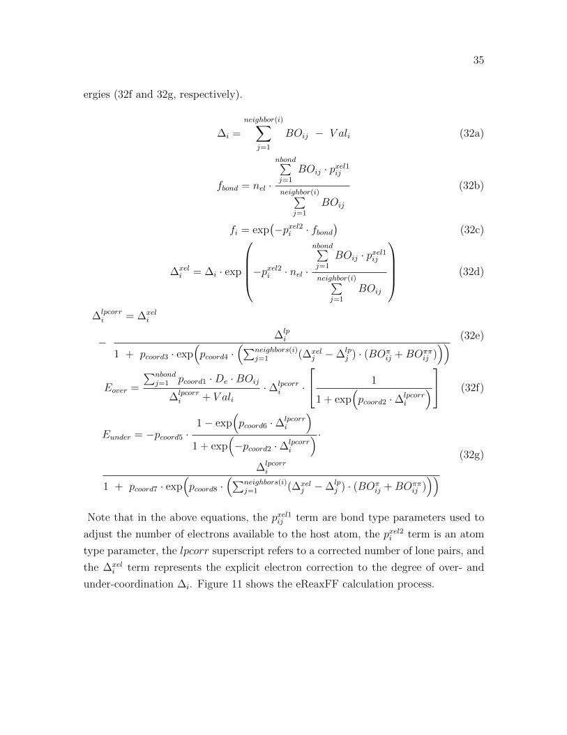
ergies (32f and 32g, respectively).
∆i =
neighbor(i)∑j=1
BOij − V ali (32a)
fbond = nel ·
nbond∑j=1
BOij · pxel1ij
neighbor(i)∑j=1
BOij
(32b)
fi = exp(−pxel2i · fbond
)(32c)
∆xeli = ∆i · exp
−pxel2i · nel ·
nbond∑j=1
BOij · pxel1ij
neighbor(i)∑j=1
BOij
(32d)
∆lpcorri = ∆xel
i
− ∆lpi
1 + pcoord3 · exp(pcoord4 ·
(∑neighbors(i)j=1 (∆xel
j −∆lpj ) · (BOπ
ij +BOππij ))) (32e)
Eover =
∑nbondj=1 pcoord1 ·De ·BOij
∆lpcorri + V ali
·∆lpcorri ·
1
1 + exp(pcoord2 ·∆lpcorr
i
) (32f)
Eunder = −pcoord5 ·1− exp
(pcoord6 ·∆lpcorr
i
)1 + exp
(−pcoord2 ·∆lpcorr
i
) ·∆lpcorri
1 + pcoord7 · exp(pcoord8 ·
(∑neighbors(i)j=1 (∆xel
j −∆lpj ) · (BOπ
ij +BOππij ))) (32g)
Note that in the above equations, the pxel1ij term are bond type parameters used to
adjust the number of electrons available to the host atom, the pxel2i term is an atom
type parameter, the lpcorr superscript refers to a corrected number of lone pairs, and
the ∆xeli term represents the explicit electron correction to the degree of over- and
under-coordination ∆i. Figure 11 shows the eReaxFF calculation process.

36
Figure 11: An illustration of the eReaxFF calculation process. The bonded and non-bondedinteractions are coupled by the explicit electron/hole description [82].
2.9 Calculating an Equilibrium Mixture, Again
The first step in using reactive force field methods is training the force field, optimizing
the parameters such as those described in Tables 5, 6, 7, 8, and 9. The training set,
as described in a 1994 paper by van Duin et al [86], must have the kind of data that
the force field is looking to produce. For example, if the force field will be used to
predict enthalpies and entropies, an appropriate training set would be experimentally
determined heats of formation.
For these calculations, since the purpose is to serve as a comparison to the CDFT
data, the CDFT energies are a perfect training set. Once the hydrocarbon force field
is optimized, a series of molecular dynamics (MD) calculations was done to obtain
another equilibrium mixture. The range of temperature values was the same as that
of the CDFT calculations. The eReaxFF software produces a file called xmolout that
keeps track of the coordinates of every atom in the system being analyzed (for the
purposes of these calculations, the free electron can be treated as an atom) as the MD
simulations run. Each MD run produced 5000 frames to be analyzed. A script was
written to calculate the distance between the electron and each of the 17 constituent
atoms of the acetophenone molecule. The number of frames in which a particular
atom was closest to the electron divided by 5000 was interpreted as the “probability”

37
of the electron being found on that atom, to allow for direct comparison with the
CDFT results.
The following section will display the results of all the calculations heretofore
described and offer interpretations in the context of all the underlying principles that
have been explained in this and the preceding section.

38
3 RESULTS
What to Make of the Work Presented Here
This third and final section serves to present the results of the research conducted
by the author and offer an interpretation thereof. This section begins by reviewing
the results of the CDFT energy calculations and the equilibrium mixture composition
obtained by using those values, then will compare that composition to the results of
the Mulliken population analysis. These results will both then be compared to the
mixture composition obtained from eReaxFF-based MD simulations. Finally, some
possibilities for future directions of this research will be addressed. These points will
all be addressed according to their relevance to the introduction and methods sections
of this work.
3.1 Constrained DFT Results
Figure 12: The acetophenone molecule, provided again for reference, adapted from [61].
Table 10 shows the relative energies for each atom state for the two hybrid func-
tionals analyzed in this thesis. The B3LYP data and the PBE0 data are quantitatively
and qualitatively similar enough that the choice of which one to use as the training
set for the reactive force field is arbitrary. The B3LYP data were chosen to train the
force field, but the PBE0 energies still serve as an illustration of the variability of the
CDFT data.

39
Atom B3LYP PBE0C1 0.086187 0.079552C2 0.044706 0.045908C3 0.000982 0.001121O4 0.382458 0.380907C5 0 0C6 0.004038 0.004072C7 0.029844 0.031194C8 0.029504 0.030804C9 0.002 0.001555H10 1.425913 1.454906H11 1.547719 1.578976H12 1.547481 1.578776H13 0.608245 0.623824H14 0.673268 0.711448H15 0.697143 0.732155H16 0.716641 0.732155H17 0.70672 0.7262
Table 10: Relative energies (eV) obtained from constrained density functional theorycalculations
Looking back at Equation 16 reveals that a lower relative energy leads to a greater
probability of the electron being found around that particular atom. When looking
at the energies, it is clear that there are three distinct tiers of electron preference: the
carbons are greatly preferred, particularly the ones that make up the benzene ring,
the lone oxygen is not very likely to host the electron, and the electron wants nothing
to do with any of the hydrogen atoms, particularly the ones outside the benzene ring.
Since the carbon atoms are the only species that show any appreciable contribution
to the mixture, Figure 13 shows the contribution of each of the carbon atoms as the
temperature increases.
The data show that the distribution smoothly becomes more uniform as the tem-
perature increases, which lines up with physical expectations: the electron will have
an easier time transitioning from state to state as thermal energy rises. Indeed, the
percentage contribution of the lone oxygen state rises from less than 10−5 at 300 K
to 0.19 at 1000 K.

40
Figure 13: The percentage chance of the electron being found around each of the particularatoms in the benzene ring at varying temperature values, according to CDFT calculations
3.2 eReaxFF-MD Results
Figure 14 shows the evolution of the equilibrium mixture composition obtained from
MD simulations. As is the case with the CDFT calculations, the only appreciable
contributions to the mixture come from the carbon atoms. Since the analysis of the
MD simulations only accounts for the closest atom to the electron in each frame,
there is no guarantee that every atom will be represented. These data indicate that
the most favorable atom state for the electron is C8, different from the C5 prediction
of the CDFT data, though, again, the MD data is less uniform across the range of
temperatures.
The general trend of the mixture composition becoming more evenly distributed
across the atom states is seen again in this data, though the increases/decreases in
percentage composition are not as uniform. This is perhaps due to the more dynamic
nature of the eReaxFF-MD calculations relative to the CDFT energy calculations,
which are performed at 0 K and then assigned a temperature to be able to calculate
a mixture composition.

41
Figure 14: The percentage chance of the electron being found around each of the particularatoms in the benzene ring at varying temperature values, according to reactive force field-based MD calculations
3.3 Mulliken Population Analysis Results
Figure 15: The acetophenone molecule, adapted from [61].
Table 11 shows the charge density results of the Mulliken population analysis for
both the neutral acetophenone molecule and the radical anion. A set of differential
Mulliken charges is necessary because, although Mulliken charges bear a passing sim-
ilarity to atomic numbers, they should not be interpreted as physical charges without
context. The differential Mulliken charge can be interpreted as the effect that the

42
Atom Neutral Anion DifferenceC1 6.33 6.32 -0.01C2 5.69 5.81 +0.12C3 6.20 6.20 -O4 8.37 8.52 +0.15C5 6.08 6.15 +0.07C6 6.03 6.10 +0.07C7 6.10 6.11 +0.01C8 6.10 6.11 +0.01C9 6.09 6.19 +0.10H10 0.85 0.92 +0.07H11 0.87 0.92 +0.05H12 0.87 0.92 +0.05H13 0.89 0.95 +0.06H14 0.87 0.92 +0.05H15 0.89 0.96 +0.07H16 0.89 0.95 +0.06H17 0.89 0.97 +0.08
Table 11: A comparison of the Mulliken charges of neutral acetophenone and theacetophenone radical anion
introduction of the electron has on the occupancy of each atom. This allows a com-
parison to the CDFT equilibrium mixture, even though the orbitals of each atom are
not completely independent the way that the atom states are in the CDFT mixture
composition calculation.
The charge differentials seen here are comparable to those obtained when different
basis sets are used. For example, the same calculation with the aforementioned cc-
pvdz basis set yields very similar results, with the largest positive increase in Mulliken
charge on the lone oxygen and substantial positive increases on the hydrogens around
the benzene ring. This assuages some fear about the basis set dependence that can
plague Mulliken population schemes.

43
3.4 Discussion
It is encouraging that the CDFT and eReaxFF-MD mixture composition results are
similar, since the CDFT energies were used to train the force field used in the MD
calculations. Their emphatic agreement that the electron prefers to situate itself in
the benzene ring is, however, slightly surprising. When looking at the constituent
pieces of the acetophenone molecule, one might expect that the lone oxygen, which
as an element is far more electronegative than carbon or hydrogen, might attract the
lone electron. However, O4 and its partner in the carbonyl group, C2, are not well-
represented in the mixture compositions. The oxygen takes some electron density
away from carbon, leaving C2 as an electrophile, but for any anion, the excess charge
would like to delocalize, not localize on C2, even if C2 is electron deficient.
The prominence of C2 and O4 is a point of disagreement between the mixture
composition calculations and the Mulliken population, in which the two atom states
have charge differentials of +0.12 and +0.15, respectively. To understand this dispar-
ity, it is necessary to understand the difference in what these two types of calculations
measure. The CDFT mixture (and the CDFT-trained MD mixture) measure the sta-
bility of each state after an extra electron that is already present in the system fixes
itself in a particular state. The Mulliken charge differential considers what happens
when a charge is introduced into the system.
So in the case of the Mulliken charge, it is reasonable that an extra electron would
be drawn to the most electronegative atom and also be drawn to the electron-seeking
carbon attached to that very electronegative atom at the end of an extremely polar
bond. And in the case of the CDFT energies, an electron that makes its way to the
lone oxygen might not stay very long because the slightly-positive C2 might pull it
away.
The hydrogen atoms in the methyl group, H10, H11, and H12, are the most
undesirable locations for the atoms according to the CDFT data. This makes sense
from a stability perspective. The carbon at the center of the methyl group is so
much more electronegative than the hydrogen atoms surrounding it that an electron
that found itself on any of those hydrogen atoms would not last long. The Mulliken
charge data shows substantial increases for this trio of hydrogen atoms after the
introduction of the electron. This may be because Mulliken population schemes
distribute electronic overlap between two atoms equally between the atoms with no
regard for characteristics of the bonded atoms, such as electronegativity. Through

44
this, the hydrogen atoms in the molecule may get a large boost to their Mulliken
charges while the carbons that they are bonded to benefit only marginally. This
same effect is seen with the hydrogen atoms in the benzene ring.
The carbon atom in the methyl group, C1, is not an attractive place for an electron
to land because its valence electrons are all tied up in bonding with the three hydro-
gens around it. The Mulliken charges show a nice symmetry around the benzene ring.
C5 and C6 have the same increase in Mulliken charge, as do C7 and C8. However, C9
sees a substantial increase, while C3 does not change at all. This is perhaps because
of the proximity in the molecular geometry of C3 to the very electron-attractive car-
bonyl group. In the CDFT energies data, C5 and C3 are the most stable atom states,
followed closely by C9 and C6.

45
3.5 Future Directions
The CDFT energies and the Mulliken populations were calculated with basis sets and
exchange-correlation functionals that could be easily changed. While work was done
to find the best combination of parameters for these calculations, changes made can
be used to perform a systematic sensitivity analysis for calculations on this system,
such as those already established by calculating the CDFT energies for the modified
B3LYP and PBE0 hybrid functionals.
As mentioned previously, in standard eReaxFF calculations, the mass of the elec-
tron or hole is taken to be one atomic mass unit, or the mass of a hydrogen atom,
following the lead of a few other computational methods that treat electrons semi-
classically [85]. In the real world, the mass of an electron is much lighter, about 104
times lighter than an atomic mass unit. While the mass of the charge carrier does
not show up in any of the equations describing the terms of the reactive force field
energies [78] [85], varying this mass could have interesting effects on how the electron
distributes itself across the molecule over the course of an MD run. At a small enough
mass, tunneling may arise, but there has been work done on evaluating the behavior
of lighter particles in molecular dynamics simulations [87].
The force field that has been developed for energy calculations on the acetophe-
none radical anion system can be put to myriad uses beyond what has been discussed
in this thesis.

46
REFERENCES
[1] J. C. Fothergill, “City Research Online City , University of London Institutional
Repository The Coming of Age of HVDC Extruded Power Cables,” Electrical
Insulation Conference (EIC), pp. 124–137, 2014.
[2] F. H. Kreuger, Industrial High Voltage, Vol 1. Delft, NL: Delft University Press,
1991.
[3] “China powers ahead with a new direct-current infrastructure,” 2017.
[4] V. Vahedy, “Polymer insulated high voltage cables,” IEEE Electrical Insulation
Magazine, vol. 22, no. 3, pp. 13–18, 2006.
[5] K. Lahti and K. Nousiainen, “Transmission Line Corona Losses under Hoar Frost
Conditions,” IEEE Transactions on Power Delivery, vol. 12, no. 2, pp. 928–933,
1997.
[6] N. Hampton, R. Hartlein, H. Lennartsson, H. Orton, and R. Ramachandran,
“Long-Life Xlpe Insulated Power Cable,” 7th International Conference on Insu-
lated Power Cable, Jicable, France, pp. 1–6, 2007.
[7] E. Y. Chen, “Coordination polymerization of polar vinyl monomers by single-site
metal catalysts,” Chemical Reviews, vol. 109, no. 11, pp. 5157–5214, 2009.
[8] O. Perez and J. B. Soares, “Coordination Polymerization,” Handbook of Polymer
Synthesis, Characterization, and Processing, pp. 85–104, 2013.
[9] C. Elschenbroich and A. Salzer, Organometallics: A Concise Introduction. New
York: VCH Verlag, 1992.
[10] C. Brown, A. Lita, Y. Tao, N. Peek, M. Crosswhite, M. Mileham, J. Krzystek,
R. Achey, R. Fu, J. K. Bindra, M. Polinski, Y. Wang, L. J. Van De Burgt,
D. Jeffcoat, S. Profeta, A. E. Stiegman, and S. L. Scott, “Mechanism of Initiation
in the Phillips Ethylene Polymerization Catalyst: Ethylene Activation by Cr(II)
and the Structure of the Resulting Active Site,” ACS Catalysis, vol. 7, no. 11,
pp. 7442–7455, 2017.
[11] HOGAN JP, “Ethylene polymerization catalysis over chromium oxide,” J Polym
Sci Part A-1 Polym Chem, vol. 8, no. 9, pp. 2637–2652, 1970.

47
[12] P. Flory, “Polymerization of Unsaturated Monomers by Free Radical Polymer-
ization,” in Principles of Polymer Chemistry, pp. 106–174, Ithaca: Cornell Uni-
versity Press, 1953.
[13] J. Cowie, “Free Radical Addition Polymerization,” in Polymers: Chemistry and
Physics of Modern Materials, pp. 52–82, London: Chapman and Hall, 2 ed.,
1991.
[14] D. B. Malpass, “Free Radical Polymerization of Ethylene,” Introduction to In-
dustrial Polyethylene, pp. 23–32, 2010.
[15] A. Peacock, Handbook of Polyethylene. New York: Marcel Dekker, 2000.
[16] K. S. Whiteley, T. G. Heggs, H. Koch, R. L. Mawer, and W. Immel, “Polyolefins,”
in Ullmann’s Encyclopedia of Industrial Chemistry, Weinheim, Germany: Wiley-
VCH Verlag GmbH & Co. KGaA, 6 2000.
[17] “Polyethyelene (PE) Plastic,” 2020.
[18] P. P. Institute, “Properly Specifying HDPE Conduit for Power and Communi-
cations Projects,” 2018.
[19] S. A. Baeurle, A. Hotta, and A. A. Gusev, “On the glassy state of multiphase
and pure polymer materials,” Polymer, vol. 47, no. 17, pp. 6243–6253, 2006.
[20] M. Nic, J. Jirat, B. Kosata, A. Jenkins, and A. McNaught, eds., Compendium
of Chemical Terminology. Research Triagle Park, NC: IUPAC, 6 2009.
[21] T. Andrews, R. N. Hampton, A. Smedberg, D. Wald, V. Waschk, and W. Weis-
senberg, “The role of degassing in XLPE power cable manufacture,” IEEE Elec-
trical Insulation Magazine, vol. 22, no. 6, pp. 5–16, 2006.
[22] S. M. Tamboli, S. T. Mhaske, and D. D. Kale, “Crosslinked polyethylene,” Indian
Journal of Chemical Technology, vol. 11, no. 6, pp. 853–864, 2004.
[23] T. O. J. Kresser, “Basic Chemistry of Polyethylene,” in Polyethylene, pp. 40–64,
New York: Reinhold Publishing Corp., 1957.
[24] Y. Badr, Z. I. Ali, A. H. Zahran, and R. M. Khafagy, “Characterization of gamma
irradiated polyethylene films by DSC and X-ray diffraction techniques,” Polymer
International, vol. 49, no. 12, pp. 1555–1560, 2000.

48
[25] A. Brandolin, “An Improved Kinetic Model for the Peroxide Initiated Mod if
icat i on of Po lye,” vol. 39, no. 10, pp. 2085–2095, 1999.
[26] C. Meola, G. M. Carlomagno, A. Squillace, U. Prisco, and R. E. Morace,
“Analysis of composites with infrared thermography,” Macromolecular Symposia,
vol. 228, pp. 273–286, 2005.
[27] T. Bremner, A. Rudin, and S. Haridoss, “Effects of polyethylene molecular struc-
ture on peroxide crosslinking of low density polyethylene,” Polymer Engineering
& Science, vol. 32, no. 14, pp. 939–943, 1992.
[28] S. Hosoda, “Structural Distribution of Linear Low-Density Polyethylenes,” Poly-
mer Journal, vol. 20, pp. 383–397, 1988.
[29] J. Sahyoun, A. Crepet, F. Gouanve, L. Keromnes, and E. Espuche, “Diffusion
mechanism of byproducts resulting from the peroxide crosslinking of polyethy-
lene,” Journal of Applied Polymer Science, vol. 134, no. 9, pp. 1–11, 2017.
[30] R. J. Coelho, “Space Charge-Limited, Injection-Controlled Conduction,” in
Physics of Dielectrics for the Engineer, pp. 123–135, Amsterdam: Elsevier Sci-
entific Pub., 1979.
[31] J. Hornak, P. Kadlec, P. Totzauer, P. Trnka, and M. Gutten, “Dielectric spec-
troscopy and absorption/resorption analysis of composite dielectric with MgO
filler,” in 18th International Scientific Conference on Electric Power Engineer-
ing (EPE), (Kouty nad Desnou, CZE), pp. 1–4, 2017.
[32] R. W. Mott, N. F.; Gurney, Electronic processes in ionic crystals. Oxford: Oxford
University Press, 1 ed., 1940.
[33] P. N. Murgatroyd, “Theory of space-charge-limited current enhanced by Frenkel
effect,” Journal of Physics D: Applied Physics, vol. 3, no. 2, pp. 151–156, 1970.
[34] N. Hussin and G. Chen, “The effect of acetophenone and alpha-methylstyrene
on the space charge properties of low density polyethylene,” Annual Report -
Conference on Electrical Insulation and Dielectric Phenomena, CEIDP, pp. 702–
705, 2008.
[35] M. Fu, G. Chen, A. Dissado, and J. C. Fothergill, “Influence of thermal treat-
ment and residues on space charge accumulation in XLPE for DC power cable
49
application,” IEEE Transactions on Dielectrics and Electrical Insulation, vol. 14,
no. 1, pp. 53–64, 2007.
[36] T. Takada, S. J. Hwang, and J. S. Noh, “Effects of constituents of XLPE on
the formation of space charge,” IEEE Transactions on Dielectrics and Electrical
Insulation, vol. 1, no. 6, pp. 1077–1083, 1994.
[37] J. V. Gulmine, P. R. Janissek, H. M. Heise, and L. Akcelrud, “Polyethylene
characterization by FTIR,” Polymer Testing, vol. 21, no. 5, pp. 557–563, 2002.
[38] M. Uhniat, M. Sudol, and S. Kudla, “Stabilization of LDPE cross-linked in
the presence of peroxides. II. FTIR study of chemical changes taking place in
the LDPE-dicumyl peroxide-Irganox 1081 system,” Polymer Degradation and
Stability, vol. 71, no. 1, pp. 75–82, 2000.
[39] P. Pinkerneil, J. Guldenhaupt, K. Gerwert, and C. Kotting, “Surface-attached
polyhistidine-tag proteins characterized by FTIR difference spectroscopy,”
ChemPhysChem, vol. 13, no. 11, pp. 2649–2653, 2012.
[40] J. V. Gulmine and L. Akcelrud, “FTIR characterization of aged XLPE,” Polymer
Testing, vol. 25, no. 7, pp. 932–942, 2006.
[41] M. Bydder, A. Rahal, G. D. Fullerton, and G. M. Bydder, “The magic angle
effect: A source of artifact, determinant of image contrast, and technique for
imaging,” Journal of Magnetic Resonance Imaging, vol. 25, no. 2, pp. 290–300,
2007.
[42] J. M. Tyszka, S. E. Fraser, and R. E. Jacobs, “Magnetic resonance microscopy:
Recent advances and applications,” Current Opinion in Biotechnology, vol. 16,
no. 1 SPEC. ISS., pp. 93–99, 2005.
[43] J. Paul, E. W. Hansen, and J. Roots, “Application of single-pulse solid-state
1H-MAS NMR to probe the oxidation products in crosslinked polyethylene: A
detailed spectral analysis procedure,” Polymer Degradation and Stability, vol. 98,
no. 1, pp. 408–415, 2013.
[44] M. Blasko, P. Mach, A. Antusek, and M. Urban, “DFT Modeling of Cross-
Linked Polyethylene: Role of Gold Atoms and Dispersion Interactions,” Journal
of Physical Chemistry A, vol. 122, no. 5, pp. 1496–1503, 2018.

50
[45] M. Golriz, H. A. Khonakdar, J. Morshedian, S. H. Jafari, Y. Mohammadi, and
U. Wagenknecht, “Microstructural evolution in linear low density polyethylene
during peroxide modification: A Monte Carlo simulation study,” Macromolecular
Theory and Simulations, vol. 22, no. 8, pp. 426–438, 2013.
[46] A. Moyassari, M. Unge, M. S. Hedenqvist, U. W. Gedde, and F. Nilsson, “First-
principle simulations of electronic structure in semicrystalline polyethylene,”
Journal of Chemical Physics, vol. 146, no. 20, 2017.
[47] S. Iwata, H. Uehara, and T. Takada, “Computational study on acetophenone in
amorphous polyethylene,” Journal of Molecular Modeling, vol. 23, no. 10, 2017.
[48] M. Meunier, N. Quirke, and A. Aslanides, “Molecular modeling of electron traps
in polymer insulators: Chemical defects and impurities,” Journal of Chemical
Physics, vol. 115, no. 6, pp. 2876–2881, 2001.
[49] D. R. Rottach, J. G. Curro, J. Budzien, G. S. Grest, C. Svaneborg, and R. Ev-
eraers, “Permanent set of cross-linking networks: Comparison of theory with
molecular dynamics simulations,” Macromolecules, vol. 39, no. 16, pp. 5521–
5530, 2006.
[50] D. R. Rottach, J. G. Curro, J. Budzien, G. S. Grest, C. Svaneborg, and R. Ev-
eraers, “Molecular dynamics simulations of polymer networks undergoing se-
quential cross-linking and scission reactions,” Macromolecules, vol. 40, no. 1,
pp. 131–139, 2007.
[51] H. Zhang, Y. Shang, M. Li, H. Zhao, X. Wang, and B. Han, “Theoretical study
on the radical reaction mechanism in the cross-linking process of polyethylene,”
RSC Advances, vol. 5, no. 110, pp. 90343–90353, 2015.
[52] D. Sholl and J. Steckel, “What is Density Functional Theory?,” in Density Func-
tional Theory: A Practical Introduction, pp. 1–34, Hoboken, NJ, USA: John
Wiley and Sons, 2009.
[53] T. Cormen, C. Leiserson, R. Rivest, and C. Stein, “Strassen’s algorithm for
matrix multiplication,” in Introduction to Algorithms, pp. 735–742, Cambridge,
MA: MIT Press, 2009.
[54] M. Born and J. Oppenheimer, “On the Quantum Theory of Molecules (Trans-
lated from German by S.M. Blinder),” Ann. Physik, vol. 84, pp. 457–484, 1927.

51
[55] L. Thomas, “The calculation of atomic fields,” Mathematical Proceedings of the
Cambridge Philosophical Society, vol. 23, no. 5, pp. 542–548, 1927.
[56] P. Hohenberg and W. Kohn, “Inhomogeneous Electron Gas,” Physical Review,
vol. 136, no. 3B, 1964.
[57] E. Kryachko and E. Ludena, “A Rigorous Formulation of the Variational Prin-
ciple in Density Functional Theory,” in Energy Density Functional Theory of
Many-Electron Systems, p. 506, Dordrecht, NL: Kluwer Academic, 1990.
[58] W. Kohn and L. Sham, “Self-Consistent Equations Including Exchange and Cor-
relation Effects,” Physical Review, vol. 140, no. 4A, 1965.
[59] B. Kaduk, T. Kowalczyk, and T. Van Voorhis, “Constrained density functional
theory,” Chemical Reviews, vol. 112, no. 1, pp. 321–370, 2012.
[60] P. H. Dederichs, S. Blgel, R. Zeller, and H. Akai, “Ground states of constrained
systems: Application to cerium impurities,” Physical Review Letters, vol. 53,
no. 26, pp. 2512–2515, 1984.
[61] “Calculated Geometries available for CH3COC6H5 (acetophenone) 1A’ Cs,”
2019.
[62] R. Ditchfield, W. J. Hehre, and J. A. Pople, “Self-consistent molecular-orbital
methods. IX. An extended gaussian-type basis for molecular-orbital studies of
organic molecules,” The Journal of Chemical Physics, vol. 54, no. 2, pp. 720–
723, 1971.
[63] D. E. Woon and T. H. Dunning, “Gaussian basis sets for use in correlated molecu-
lar calculations. V. Core-valence basis sets for boron through neon,” The Journal
of Chemical Physics, vol. 103, no. 11, pp. 4572–4585, 1995.
[64] E. R. Davidson and D. Feller, “Basis Set Selection for Molecular Calculations,”
Chemical Reviews, vol. 86, no. 4, pp. 681–696, 1986.
[65] J. P. Perdew, M. Ernzerhof, and K. Burke, “Rationale for mixing exact exchange
with density functional approximations,” Journal of Chemical Physics, vol. 105,
no. 22, pp. 9982–9985, 1996.

52
[66] A. D. Becke, “Perspective: Fifty years of density-functional theory in chemical
physics,” Journal of Chemical Physics, vol. 140, no. 18, 2014.
[67] J. P. Perdew, J. A. Chevary, S. H. Vosko, K. A. Jackson, M. R. Pederson, D. J.
Singh, and C. Fiolhais, “Erratum: Atoms, molecules, solids, and surfaces: Appli-
cations of the generalized gradient approximation for exchange and correlation
(Physical Review B (1993) 48, 7, (4978)),” Physical Review B, vol. 48, no. 7,
p. 4978, 1993.
[68] S. H. Vosko, L. Wilk, and M. Nusair, “Accurate spin-dependent electron liq-
uid correlation energies for local spin density calculations: a critical analysis,”
Canadian Journal of Physics, vol. 58, no. 8, pp. 1200–1211, 1980.
[69] A. D. Becke, “Density-functional thermochemistry. III. The role of exact ex-
change,” The Journal of Chemical Physics, vol. 98, no. 7, pp. 5648–5652, 1993.
[70] J. P. Perdew, K. Burke, and M. Ernzerhof, “Generalized gradient approximation
made simple,” Physical Review Letters, vol. 77, no. 18, pp. 3865–3868, 1996.
[71] M. C. Kim, E. Sim, and K. Burke, “Communication: Avoiding unbound anions
in density functional calculations,” Journal of Chemical Physics, vol. 134, no. 17,
pp. 4–7, 2011.
[72] R. Kar, J. W. Song, and K. Hirao, “Long-range corrected functionals satisfy
Koopmans’ theorem: Calculation of correlation and relaxation energies,” Journal
of Computational Chemistry, vol. 34, no. 11, pp. 958–964, 2013.
[73] E. Apra, E. J. Bylaska, W. A. de Jong, N. Govind, K. Kowalski, T. P. Straatsma,
M. Valiev, H. J. van Dam, Y. Alexeev, J. Anchell, V. Anisimov, F. W. Aquino,
R. Atta-Fynn, J. Autschbach, N. P. Bauman, J. C. Becca, D. E. Bernholdt,
K. Bhaskaran-Nair, S. Bogatko, P. Borowski, J. Boschen, J. Brabec, A. Bruner,
E. Cauet, Y. Chen, G. N. Chuev, C. J. Cramer, J. Daily, M. J. Deegan, T. H.
Dunning, M. Dupuis, K. G. Dyall, G. I. Fann, S. A. Fischer, A. Fonari, H. Fruchtl,
L. Gagliardi, J. Garza, N. Gawande, S. Ghosh, K. Glaesemann, A. W. Gotz,
J. Hammond, V. Helms, E. D. Hermes, K. Hirao, S. Hirata, M. Jacquelin,
L. Jensen, B. G. Johnson, H. Jonsson, R. A. Kendall, M. Klemm, R. Kobayashi,
V. Konkov, S. Krishnamoorthy, M. Krishnan, Z. Lin, R. D. Lins, R. J. Little-
field, A. J. Logsdail, K. Lopata, W. Ma, A. V. Marenich, J. Martin Del Campo,

53
D. Mejia-Rodriguez, J. E. Moore, J. M. Mullin, T. Nakajima, D. R. Nascimento,
J. A. Nichols, P. J. Nichols, J. Nieplocha, A. Otero-de-la Roza, B. Palmer, A. Pa-
nyala, T. Pirojsirikul, B. Peng, R. Peverati, J. Pittner, L. Pollack, R. M. Richard,
P. Sadayappan, G. C. Schatz, W. A. Shelton, D. W. Silverstein, D. M. Smith,
T. A. Soares, D. Song, M. Swart, H. L. Taylor, G. S. Thomas, V. Tipparaju,
D. G. Truhlar, K. Tsemekhman, T. Van Voorhis, Vazquez-Mayagoitia, P. Verma,
O. Villa, A. Vishnu, K. D. Vogiatzis, D. Wang, J. H. Weare, M. J. Williamson,
T. L. Windus, K. Wolinski, A. T. Wong, Q. Wu, C. Yang, Q. Yu, M. Zacharias,
Z. Zhang, Y. Zhao, and R. J. Harrison, “NWChem: Past, present, and future,”
The Journal of chemical physics, vol. 152, no. 18, p. 184102, 2020.
[74] A. C. Van Duin, J. M. Baas, B. Van De Graaf, J. W. De Leeuw, T. P. Bastow,
and R. Alexander, “Comparison of calculated equilibrium mixtures of alkylnaph-
thalenes and alkylphenanthrenes with experimental and sedimentary data; the
importance of entropy calculations,” Organic Geochemistry, vol. 26, no. 3-4,
pp. 275–280, 1997.
[75] R. S. Mulliken, “Electronic Population Analysis on LCAO,” J. Chem. Phys,
vol. 23, no. January 1955, p. 1833, 1955.
[76] P. O. Lowdin, “On the non-orthogonality problem connected with the use of
atomic wave functions in the theory of molecules and crystals,” The Journal of
Chemical Physics, vol. 18, no. 3, pp. 365–375, 1950.
[77] G. Bruhn, E. R. Davidson, I. Mayer, and A. E. Clark, “Lowdin Population
Analysis With and Without Rotational Invariance,” International Journal of
Quantum Chemistry, vol. 106, pp. 2065–2072, 2006.
[78] A. C. Van Duin, S. Dasgupta, F. Lorant, and W. A. Goddard, “ReaxFF: A
reactive force field for hydrocarbons,” Journal of Physical Chemistry A, vol. 105,
no. 41, pp. 9396–9409, 2001.
[79] D. W. Brenner, “Empirical potential for hydrocarbons for use in simulating the
chemical vapor deposition of diamond films,” Physical Review B, vol. 42, no. 15,
pp. 9458–9471, 1990.
[80] H. S. Johnston and C. Parr, “Activation Energies from Bond Energies. I. Hy-
drogen Transfer Reactions,” Journal of the American Chemical Society, vol. 85,
no. 17, pp. 2544–2551, 1963.
54
[81] D. M. Root, C. R. Landis, and T. Cleveland, “Valence Bond Concepts Applied
to the Molecular Mechanics Description of Molecular Shapes. 1. Application to
Nonhypervalent Molecules of the P-Block,” Journal of the American Chemical
Society, vol. 115, no. 10, pp. 4201–4209, 1993.
[82] T. P. Senftle, S. Hong, M. M. Islam, S. B. Kylasa, Y. Zheng, Y. K. Shin,
C. Junkermeier, R. Engel-Herbert, M. J. Janik, H. M. Aktulga, T. Verstraelen,
A. Grama, and A. C. Van Duin, “The ReaxFF reactive force-field: Develop-
ment, applications and future directions,” npj Computational Materials, vol. 2,
no. November 2015, 2016.
[83] W. J. Mortier, S. K. Ghosh, and S. Shankar, “Electronegativity Equalization
Method for the Calculation of Atomic Charges in Molecules,” Journal of the
American Chemical Society, vol. 108, no. 15, pp. 4315–4320, 1986.
[84] D. Bedrov, G. D. Smith, and A. C. Van Duin, “Reactions of singly-reduced ethy-
lene carbonate in lithium battery electrolytes: A molecular dynamics simulation
study using the ReaxFF,” Journal of Physical Chemistry A, vol. 116, no. 11,
pp. 2978–2985, 2012.
[85] M. M. Islam, G. Kolesov, T. Verstraelen, E. Kaxiras, and A. C. Van Duin,
“EReaxFF: A Pseudoclassical Treatment of Explicit Electrons within Reactive
Force Field Simulations,” Journal of Chemical Theory and Computation, vol. 12,
no. 8, pp. 3463–3472, 2016.
[86] A. C. Van Duin, J. M. Baas, and B. Van De Graaf, “Delft molecular mechanics:
A new approach to hydrocarbon force fields. Inclusion of a geometry-dependent
charge calculation,” Journal of the Chemical Society, Faraday Transactions,
vol. 90, no. 19, pp. 2881–2895, 1994.
[87] M. Ceriotti, M. Parrinello, T. E. Markland, and D. E. Manolopoulos, “Effi-
cient stochastic thermostatting of path integral molecular dynamics,” Journal of
Chemical Physics, vol. 133, no. 12, 2010.