the 2009 recovery act and the expected in ation channel of
TRANSCRIPT

The 2009 Recovery Act and the Expected Inflation Channel of
Government Spending∗
Bill Dupor†and Rong Li‡
January 23, 2014
Abstract
There exist sticky price models in which the output response to a government spending changecan be large if the central bank is nonresponsive to inflation. According to this “expectedinflation channel,” government spending drives up expected inflation, which in turn, reducesthe real interest rate and leads to an increase in private consumption. This paper examineswhether the channel was important in the post-WWII U.S., with particular attention to the2009 Recovery Act period. First, we show that a model calibrated to have a large outputmultiplier requires a large response of expected inflation to a government spending shock. Next,we show that this large response is inconsistent with structural vector autoregression evidencefrom the Federal Reserve’s passive policy period (1959-1979). Then, we study expected inflationmeasures during the Recovery Act period in conjunction with a panel of professional forecastersurveys, a cross-country comparison of bond yields and fiscal policy news announcements. Weshow that the expected inflation response was too small to engender a large output multiplier.
Keywords: monetary policy, fiscal policy, output multipliers, 2009 Recovery Act.
JEL Codes: E52, E62.
∗The authors thank Charles Carlstrom, John Cochrane, Paul Evans and Patrick Kehoe as well as seminar participants at the
Federal Reserve Bank of Richmond for useful comments. The authors also thank Peter McCrory for helpful research assistance.
A repository containing government documents, data sources, a bibliography and other relevant information pertaining to the
Recovery Act is available at billdupor.weebly.com. The analysis set forth does not reflect the views of the Federal Reserve Bank
of St. Louis or the Federal Reserve System. First draft: April 2013.†Federal Reserve Bank of St. Louis, [email protected], [email protected].‡The Ohio State University, [email protected].
1

1 Introduction
In February 2009, the U.S. government began mounting a massive fiscal stimulus program: the
American Recovery and Reinvestment Act, also known as the Recovery Act. The Congressional
Budget Office’s most recent assessment is that the Act’s budget impact will total $830 billion.
Government consumption and investment made up roughly $250 billion of the Act’s spending: the
remainder consisted of tax cuts, tax incentives and entitlements. While some analysts have argued
that the Act had a strong positive impact on the macroeconomy (e.g. Blinder and Zandi (2010) and
Council of Economic Advisers (various quarterly reports)), the workhorse neoclassical growth model
implies that stimulative government-spending policy has a muted effect on total economic activity.
In that model, increased government spending reduces households’ after-tax lifetime income, which
leads them to reduce consumption. In the language of introductory macro textbooks, government
spending “crowds out” consumption and the “output multiplier” is less than 1.
A number of researchers have posited that there exists an expected inflation channel for govern-
ment spending, in which consumption rises rather than falls.1 According to this channel, govern-
ment spending drives up the current and expected future real wage. If a business may be unable
to change its price for some duration, the shift up in its expected real wage path leads the business
to increase its price today. This shift will generate expected inflation which, in turn, reduces the
expected real rate; such a reduction leads households to shift consumption toward the present.
This effect is particularly strong when a central bank does not react to inflation by tightening its
monetary policy. One reason that a central bank might be unresponsive is that a zero lower bound
on the nominal rate may be binding.
Some have contended that the channel was important during particular historical episodes.
Eggertsson (2012) examines this channel in the context of the New Deal and concludes that it helped
end the Great Depression. Christiano, Eichenbaum and Rebelo (2011) examine the mechanism
during the 2009 Recovery Act period and conclude that it had an output multiplier as high as 2.3.
In light of the limitations on monetary policy because of the zero lower bound (ZLB), the
Recovery Act may seem an ideal catalyst for the expected inflation channel. First, it was a massive
program. For example, highway and bridge construction and improvement funded by the Act was
$28 billion; this equaled 76% of 2008 federal-aid highway dollars ($36.9 billion). Without the Act,
wages in this part of the construction industry might have been substantially lower, thus exerting
downward pressure on inflation. As a second example, the Act allocated over $50 billion to pay
public school teachers and other government workers. Without this component, it is likely that fewer
government employees would have been added to payrolls, fewer would have received pay raises,
some layoffs would have occurred and government furloughs would have been more common. This
could have conceivably driven down wages in the government sector, putting downward pressure
1See for example Christiano (2004), Christiano, Eichenbaum and Rebelo (2011), Eggertsson (2004), Erceg andLinde (2010) and Woodford (2011). The phrase we use to describe this channel is of our making.
2
on inflation.
The Act also introduced inefficient “wedges” into the economy, which act like negative “supply”
shocks, and might have put upward pressure on inflation. For example, the Davis-Bacon require-
ments in the Act required private contractors on many of the Act’s projects to pay “prevailing
wages,” which are often tied to union-negotiated pay scales. Through this and other wedges, the
Act may have helped prevent downward pressure on the market wage and thus inflation.
This paper answers a narrow question: did the expected inflation channel engender a large
output multiplier during periods of monetary accommodation in the post-WWII U.S.?2
We execute two distinct strategies to measure the magnitude of the expected inflation chan-
nel. Neither strategy finds a quantitatively important effect. Our first strategy stems from an
observation about the New Keynesian paradigm: large output multipliers arise through the non-
responsiveness of the central bank’s interest rate; the zero-lower bound is simply one basis for
non-responsiveness. We observe that monetary policy was much less responsive to inflation in the
20 years preceding 1980 than in the twenty years that followed. As such, the expected inflation
channel hypothesis implies that inflation should respond more to government spending shocks in
the earlier, relative to the later, period.
Using a sticky price model (as typically calibrated), we show how the multiplier is much larger
under a passive (relative to an active) monetary policy. Then, we examine the data from the two
periods, specifically 1959-79 and 1981-2002. We identify impulse responses to government spending
shocks using stock return data on U.S. military contractors, following Fisher and Peters (2010).
During the passive policy period, there is a -8 bp one-year inflation response to a Recovery Act
sized spending shock. The corresponding response during the active period is -176 bp. Neither of
the two periods show support for the expected inflation channel: inflation falls rather than rises
in response to positive spending shocks. Moreover, we find a statistically insignificant response of
consumption to government spending at all horizons, which is also consistent with a weak expected
inflation channel.
For the second strategy, we begin by calibrating a model which has a transitorily non-responsive
monetary policy (e.g., a ZLB constraint is temporarily binding) such that it generates a large output
multiplier. We then calculate and record the model’s expected inflation response to a Recovery Act
sized spending shock. In our baseline calibration, the implied one-year expected inflation response
is roughly 4.6%, which we view as very large.
Next we turn to the data on actual and expected inflation during the Recovery Act episode.
Actual inflation changed very little during the entire episode, both pre- and post-passage of the Act.
The U.S. had not entered into a deflationary spiral before the passage (as well as the preceding
months during which news of a federal spending program developed), nor did it experience a
2Broader questions, such as whether the Act stimulated economic activity through some other mechanism orwhether the expected inflation channel was quantitatively important during other historical episodes, are touched ononly briefly in this paper.
3

noticeable inflation increase after its passage. Since actual inflation changed very little, one would
expect the mechanism to be manifested in expected inflation.
Here is what the data tell us. From before to after enactment, the median forecast of expected
inflation from the Survey of Professional Forecasters (hereafter SPF) showed a small increase—an
order of magnitude smaller than implied by the calibrated sticky price model. Moreover, across
the panel of individual surveyed forecasters, there was no systematic increase in inflation expec-
tations by a forecaster and that forecaster’s measured increase in expected government spending
growth. That is, forecasters predicting a large stimulus were no more likely to revise their inflation
projections substantially upward.
We also measure inflation expectation from bond markets. “Break-even inflation” in a country
is calculated as the spread between nominal and indexed government bond yields in that country.
During the news/passage of the Act, break-even inflation in the U.S. and U.K. tracked each other
closely. This is telling because the U.K. did not enact, nor did it ever approach enacting, a fiscal
stimulus program during this time frame. In addition, we show that U.S. break-even inflation
moved very little on days of important fiscal policy news during the development of and legislating
on the Recovery Act.
The outline of the paper follows. Section 2 uses the behavior of pre- and post-1980 monetary
policy to assess the importance of the expected inflation channel of fiscal policy. Section 3 builds a
sticky price model and calculates the inflation and output responses to a Recovery Act size spending
policy under several alternative scenarios and then catalogs evidence on expected inflation pre- and
post-passage of the Recovery Act. Section 4 discusses existing research and Section 5 concludes.
2 The Passive Policy Era: Theory and Evidence
2.1 A Sticky Price Model with Passive Policy
Consider the following log-linearized sticky price model:
it − Et (πt+1) = σ [E (ct+1)− ct] (2.1)
πt = βEt (πt+1) + κ (σct + νyt) (2.2)
yt = (1− s) ct + sgt (2.3)
where ct, yt, πt, it and gt are, respectively, the log deviations of consumption, output, inflation, the
nominal interest rate and government spending from their corresponding steady-state values.3 For
simplicity, assume steady-state net inflation equals zero. Assume further that government spending
is financed by lump-sum taxes.
3Here σ, v and κ are non-negative and β and s lie inside the unit interval. The model set up and notation followCarlstrom, Fuerst and Paustian (2012).
4

Substituting yt out of (2.2) using (2.3), we have
πt = βEt (πt+1) + χct + ωgt (2.4)
where χ = κ (σ + v (1− s)) and ω = κsv. In the following two subsections, we describe two alter-
native monetary policies.
Large output multipliers arise through the weak response of the central bank’s interest rate to
inflation. Boivin and Giannoni (2006) and Clarida, Gali and Gertler (2000), among others, provide
evidence that monetary policy was passive (i.e. partially non-responsive) during part of the post-
WWII period. This episode will help us evalute the expected inflation channel because we have
decades of data under which U.S. monetary policy was passive (1959-79), as well as decades under
which policy was active (1981-2002). Moreover, existing methods for identifying exogenous shocks
to government spending will allow us to compute the response of inflation to spending shocks. With
the identified impulse responses, we will quantify the expected inflation channel.
Returning to the model, imagine monetary and fiscal policy are set according to
it = (ψ + 1)Et (πt+1) and gt = ρgt−1 + εt (2.5)
where εt is mean zero white noise. Policy is active when ψ > 0 and passive when ψ < 0. Here, we
following existing research and model these policies such that agents behave as if the passive policy
will remain in place forever.
Thus, we have 3 endogenous variables {ct, it, πt} in 3 equations, (2.1), (2.4) and (2.5). Using the
method of undetermined coefficients, we can solve for the model’s rational expectations equilibria
close to its steady state. For an active policy, the equilibrium is typically unique.4 Under passive
policies, the equilibrium is not unique. For this case, we follow Boivin and Giannoni (2006) and
analyze the “minimum state variable” or bubble-free equilibrium.
For both active and passive rules, inflation and output in equilibrium are given by
πt = αgt =ω (1− ρ)
β (ρ2 + θρ+ β−1)gt (2.6)
ct = γgt = χ−1 [(1− βρ)α− ω] gt (2.7)
where θ = β−1(σ−1χψ − β − 1
).
The response coefficients α and γ change with the responsiveness of monetary policy as one
would predict. Letting α = α (ψ), one can show first that α (0) = ω/ (1− βρ) > 0. Thus, for
a policy that raises the nominal rate one for one with expected inflation (often called a neutral
policy), a government spending shock will increase inflation. Also, within a range of ψ that contains
4For very large (and typically argued unrealistic) values of ψ, active policies can result in indeterminacy. We avoidthis region of the parameter space in the numerical exercises that follow.
5
zero,(ψ, ψ
), one can show that α (ψ) > 0 and α′ (ψ) < 0.
Thus, within this range, (i) government spending shocks are inflationary for both active and
passive policies, and (ii) a more passive policy results in a greater inflation response. Panel (a) of
Figure 1 represents these features diagrammatically.
Next, panel (b) of Figure 1 plots how the consumption response depends on monetary policy,
that is γ = γ (ψ). The diagram shows that γ (0) = 0, and γ′ (ψ) < 0 within a neighborhood of
ψ = 0. Thus, consumption does not respond to government spending shocks if monetary policy is
neutral; active policy implies consumption decreases in response to a positive government spending
shock; passive policy implies consumption increases in response to a positive government spending
shock. Furthermore, within some range, the consumption response is monotonically decreasing in
ψ.
Next, we proceed by quantifying the effect of varying the degree of accommodation, which
requires setting numerical values for the parameters. We set ψA = 0.5 and ψP = −0.5 for the
active and passive policies, respectively. We set ρ = 0.75. Next, the magnitude of the εt shock is
chosen so that the resulting cumulative increase in g equals 10% of one year’s level of steady-state
government spending.5 The next four parameters are set as:
β = 0.995, s = 0.2, σ = 1, v = 4
We report results for several different values of κ, the parameter dictating the response of inflation
to marginal cost.
The first choice of κ is 0.02. The calculations of α and γ appear in Table 1. For the passive
rule, the cumulative output multiplier equals 1.75; for the active rule, the corresponding value is
0.75. As under transiently fixed-rate rules (e.g. at the zero lower bound), an enduring passive
policy implies that the real interest rate is allowed to fall when government spending drives up
marginal cost, and, therefore, expected inflation. The fall in the real interest rate leads households
to increase current consumption.
The inflation response is larger under the passive rule, relative to the active rule. In response
to a Recovery Act sized shock, the 1-year inflation rate is 3.42% under the passive rule in contrast
to 1.15% under the active rule.
Next, we ask what value the output multiplier would take in the model economy where, all
other things equal, a passive monetary policy accounted for a similar size increase in the inflation
response. The next entries in Table 1 show that, when κ = 0.01, the inflation response is 0.46
percentage points larger (i.e. 1.15%-0.69%) under the passive rule. The corresponding difference
in output multipliers is 0.40 (that is, 1.25-0.85). Thus, the expected inflation channel is operative
when policy is passive, however; quantitatively it accounts for only a small change in the multiplier
when the inflation response is set at a moderate level.
5The scale of the shock is set to match the size of the spending component of the 2009 Recovery Act.
6

Figure 1: Equilibrium impact responses of inflation and consumption to a government spendingshock under active (ψ > 0) and passive (ψ < 0) rules
ω
1 − βρ
γ(Ψ)
0
(0,0)
(0,0)0
Ψ
Ψ, Response
of real rate to
expected inflation
α(Ψ)
α,
Response
of inflation
γ,
Response of
consumption
(a)
(b)
7

Table 1: Responses to a Recovery Act size government spending shock under enduring passive andactive interest rate policies.
between 2009 and 2011. Over these years, government spending was 3.61%, 4.24% and 1.11% above
its 2008 level. On average, spending was 3.0% above its 2008 level during each of the three years.
The second calibration is based on the ratio of the spending component of the Recovery Act to total
government spending in 2008. The Recovery Board reports that $250 billion of the Act’s $840 billion
were in the form of neither entitlements nor tax benefits.16 Thus, the spending component was 10% of
the total government consumption and investment in 2008. This equals a 3.3% increase an annual
amount, since the Act’s spending was spread out over (roughly) three years. The difference between
the two calibrations is likely due to the fact that some state and local governments cut back on their
own contributions to expenditures. In absence of the Recovery Act, these non‐Federal government cut
backs would have likely occurred in any case. As such, our benchmark calibration will be based on the
3.3% number.
Table: Expected output multiplier and price‐level responses to a government spending shock
under active and passive interest rate policies. The price‐level responses are with respect to a
shock with cumulative expected government spending equal to 10% of one‐year’s steady‐state
government spending.
Type of monetary policy
Expected one‐year price level response
Output multiplier (cumulative)
κ = 0.02
Passive 3.42% 1.75
Active 1.15% 0.75
κ = 0.01
Passive 1.15% 1.25
Active 0.69% 0.85
κ = 0.04
Passive 500% 110
Active 1.73% 0.62
Notes: The government spending process is AR(1) with coefficient 0.75. κ is the coefficient on
marginal cost in the inflation Euler equation.
2008-01-01 2497.412
2009-01-01 2589.370
2010-01-01 2605.813
2011-01-01 2523.851
2012-01-01 2481.700 16 Note that a few of the expenditure categorizations are necessarily somewhat arbitrary. For example, a $5.6 billion grant to states for low‐income housing is treated as an entitlement by the Recovery Board although it might equally well be treated as expenditure
Notes: The government spending process is AR(1) with coefficient 0.75. κ is the coefficient on marginal
cost in the inflation Euler equation. The price level responses are with respect to a shock with expected,
cumulative magnitude equal to 10% of one-year’s steady-state government spending.
As a final illustration, we report the same statistics, except we set κ = 0.04. Under the passive
rule, the multiplier becomes extremely large: one unit of additional government spending results in
110 additional units of output. This extremely large output multiplier is supported by an extremely
large inflation response. For this calibration, the one-year inflation rate 500% in response to the
Recovery Act sized spending shock.
2.2 Evidence from the Passive Policy Era
The numbers in Table 1 give predictions for output multipliers and inflation responses with respect
to a spending shock in a sticky price model under passive or active policies. Next, we compare
these numbers with those from U.S. data using a suitably identified estimation strategy.
We wish to estimate the structural responses to government spending shocks without imposing
too many restrictions from economic theory. We follow Fisher and Peters (2010), who identify
these shocks using the total excess returns of a portfolio of corporations that are major U.S. defense
contractors.
The excess return of defense contractors satisfies the two criteria for a sound instrument. First,
it is correlated with our endogenous variable because: (i) defense spending is a substantial compo-
nent of overall government spending, and (ii) defense contractors tend to earn above market returns
when there are positive innovations to government spending. Second, the instrument is plausibly
exogenous with respect to the error term because defense spending is driven mainly by interna-
tional geopolitical factors rather than the U.S. business cycle. Moreover, because stock prices are
8

forward-looking, the Fisher and Peters (2010) instrument is capable of capturing the news aspect of
government spending shocks unlike a number of alternative approaches, e.g. some based on time-0
recursive identification.
Our construction of the defense contractors’ excess returns follows Fisher and Peters (2010)
almost exactly6; as such, we describe the construction briefly here and direct interested readers to
their paper for greater detail. Since 1956, the U.S. Department of Defense has published annual
reports of the 100 companies that are top military contractors by dollar volume. These reports, with
a few modifications used by Fisher and Peters (2010), provide the data to construct the portfolio
of large military suppliers. First, companies are removed from the list if their primary source of
revenue is not defense (e.g. AT&T). Then, companies are removed if they were not one of the
top three contractors within at least one month over the entire period. The remaining companies
are listed in Table 1 of Fisher and Peters (2010). The portfolio of defense contractors is then the
market-capitalization-weighted sum of the remaining firms.
Our benchmark specification includes the following variables: accumulated excess returns for
key defense firms, real total government purchases, real personal consumption spending, the core
CPI level, a linear trend and a constant.
All of the variables are included in natural log form. Government purchases consist of de-
seasonalized consumption and investment of federal, local and state governments. When an original
series is measured quarterly, we linearly interpolate between each pair of quarterly observations to
construct monthly values.
The source for consumption is the monthly Personal Consumption Expenditure survey. We
deflate by the CPI to obtain a real variable. Our inflation measure in each month is computed as
the annualized three-month growth rate of the core CPI. We exclude food and energy from our
inflation measure; in addition, we use the three-month rather than the one-month growth in the
price index with the aim of smoothing out very transient movements in inflation.
Our passive (monetary policy) period covers 1959:1-1979:12; our active (monetary policy) period
consists of 1981:10-2002:6. The first period corresponds roughly to a time when policy was overly
accommodative of inflation, as described in Taylor (1999). Our dividing point between passive and
active periods corresponds to the ascendancy of Paul Volcker as chairman of the Federal Reserve.
We chose the end date for the active period based on the analysis by Taylor (2007). Taylor (2007)
writes that between early 2002 and 2005, “no greater or more persistent deviation of actual Fed
policy [from the Taylor rule] had been seen since the turbulent days of the 1970s” (p. 2).
We use nine lags, as chosen by the Akaike information criterion, for each sample.
Panels (a) and (b) of Figure 2 plot the impulse responses of government spending to an in-
novation to accumulated excess returns for each period. The size of the shock that fed into the
system is selected so that the government spending increase is comparable to the Recovery Act.
6They compute quarterly returns, whereas we compute monthly returns.
9

Table 2: Estimate of the one-year inflation response (APR) to a Recovery Act sized governmentspending shock and the consumption multiplier, from structural vector autoregression, for alterna-tive sample periods
Sample period One-year inflation response Consumption multiplier
Passive -0.08 0.32(-1.39 , 1.65) (-1.57 , 1.73)
Active -1.76 1.76(-8.86 , 5.24) (-1.35 , 4.27)
Notes: Median estimates from 500 bootstrap simulations. Corresponding 90% confidence intervals appear
in parentheses.
In particular, for each sample the cumulative spending increase during the first three years equals
10% of one year of typical government spending.
Panel (a) shows that the shock generates a hump-shaped response of spending during the passive
policy period. Initially, there is almost no effect on spending. It reaches a plateau at month 13 and
remains near the plateau for another 18 months. Spending then monotonically returns to roughly
its steady state by the end of year 4. The dashed lines envelope the pointwise 68% confidence
interval.
The impulse response in Figure 2(a) is encouraging for two reasons. First, the responses are
very similar, apart from a different scaling of the shock, to the corresponding figure in Fisher
and Peters (2010), despite the fact that: (i) they use a longer sample (1957-2007), (ii) use a
quarterly frequency, and (iii) select somewhat different variables into their vector autoregression.
Our estimates also line up qualitatively with those based on the ‘war news’ narrative approach
taken by Ramey (2011) and Ramey and Shapiro (1998). Second, the impulse response also has
the qualitative shape of the spending path authorized by the Recovery Act. Specifically, the news
of the Democratic presidential and congressional victories provided an innovation to expectations
about future government spending. This spending took many months to ramp up, followed by
several years of relatively consistent spending followed by a gradual winding down.
In contrast, exogenous spending identified by an alternative approach based on timing restric-
tions (e.g. Auerbach and Gorodnichenko (2012)) has not exhibited hump-shaped paths for spend-
ing. In the alternative approach, the typical pattern is that spending jumps up on impact and then
smoothly returns to it steady state over time.
Panel (b) of Figure 2 contains the spending impulse response for the active policy sample. It is
also hump-shaped; however, it takes significantly longer for spending to reach its peak (four years)
and much longer for spending to converge to the steady state. Thus, the pre-1980 military-driven
spending changes were less persistent than those from after 1982.
10

Figure 2: Impulse responses to a shock to the accumulated excess returns on a portfolio of majorU.S. military contractors from a structural vector autoregression, for alterative sample periods, inpercentage deviation terms
10 20 30 40−5
0
5
10
Gov
. spe
ndin
g
(a) Passive period
10 20 30 40−5
0
5
10
Gov
. spe
ndin
g
(b) Active period
10 20 30 40
−5
0
5
Pric
e le
vel
(c) Passive period
10 20 30 40
−5
0
5P
rice
leve
l(d) Active period
10 20 30 40−10
−5
0
5
10
Con
sum
ptio
n
(e) Passive period
Month10 20 30 40
−10
−5
0
5
10
Con
sum
ptio
n
(f) Active period
Month
Notes: The passive period is 1959-79; the active period is 1981-2002. The size of the excess return shock is
chosen such that, in each period, the cumulative response of government spending over the first three years
equals 10% of one year of average spending. The dashed lines envelope the 68% confidence intervals.
11

In comparing the two samples, we seek to assess the importance of the expected inflation channel
by examining a period when it should be strong (1959-79) to a period when it should be relatively
weak (1981-2002).
Figure 2(c) shows the impulse response for the price level during the passive policy sample. The
point estimates show that, for a government spending stimulus roughly the size of the Recovery
Act, the price level increased slightly and then fell over the first two years following the start of the
spending increase. This occurred despite the fact that monetary policy was highly accommodative
during this entire time span. The 68% confidence interval contains the zero response throughout
the four-year horizon.
Recapping, several existing papers have argued that government spending has a particularly
large effect on economic activity when the nominal interest rate is stuck at zero; however, it occurs
more generally than simply when the nominal rate equals zero. It also occurs when monetary
policy is passive. The channel works because government spending drives down the real rate
through an increase in expected inflation. Figure 2(c) shows that increased government spending
from an exogenous source did not cause substantial inflation during the passive policy era. Table 2
summarizes key statistics from the impulse responses. The point estimate of the one-year inflation
response to the spending shock is -0.08% with a 90% confidence interval of (-1.39,1.65).
This response is substantially smaller than that suggested by the calibrated sticky price model.
Table 1 (with κ = 0.02) shows that in order to generate an output multiplier of 1.75, the one-year
expected inflation would increase by 3.42%.
Figure 2(d) presents the inflation response during the active monetary policy sample. The price-
level response is negative throughout the first four-years. Examining the corresponding confidence
band, we reject the hypothesis that the price level increased in response to the excess return shock
at the 68% level. Table 2 reports the point estimate and 90% confidence interval for the one-year
inflation response. At the 12-month mark following the shock, the point estimate implies that the
price level falls by 1.76%. The 90% confidence interval is extremely wide (-8.86,5.24). At this
confidence level, we conclude that the data and identification strategy are not very informative
about the expected inflation channel during the active policy period.
Panels (e) and (f) plot the consumption responses for the two samples. Using these impulse
responses, it is straightforward to calculate the estimated (cumulative) consumption multipliers.7
The estimates are not very informative for either sample. The 90% confidence interval for the
multiplier is (-1.57,1.73) for the passive policy period and (-1.35,4.27) for the active policy period
(see Table 2). We cannot reject a zero or negative response of consumption. However, we also
cannot reject a large multiplier.
On its own, the VAR evidence does not reject a large consumption multiplier; however, the
estimates do reject the expected inflation channel as a quantitatively important mechanism by
7See Section 2.1.
12

which a large consumption multiplier might have been generated.
2.3 Robustness
Next, we conduct robustness checks of our VAR analysis. Overall, the key finding from our bench-
mark specification-that the empirical inflation response to a spending shock in the passive period is
too small to support a large output multiplier-is confirmed in the alternative specifications. Table
3 contains the inflation responses. Table 4 contains the consumption responses. We focus our dis-
cussion below on the inflation response during the passive policy period because this is where the
expected inflation channel hypothesis suggests that we should find the greatest response. The first
row of Table 4 restates the benchmark finding. The bottom row of the table reports the inflation
responses from the large-multiplier calibration of the sticky price model.
The second row displays modifications of the benchmark specification by moving to a 12 lag
VAR. The point estimates in both passive and active policy periods are consistent with our bench-
mark results. The confidence intervals are wider relative to the benchmark specification.
The third and fourth rows contain modifications of the benchmark specification by moving to
either 9 or 12 lags in the VAR, and replacing CPI level with CPI inflation. For each case, the
point estimate under in the passive rule is nearly unchanged and the confidence interval tightens
relative to the benchmark specification. For the active period, we find a higher inflation response
and consumption multiplier; however, they are also inconsistent with large multiplier sticky price
calibration. Moreover, with 9 lags, the 90% confidence interval for the consumption multiplier is
(-11.53, 11.58). We cannot reject a zero or negative response of consumption. However, we also
cannot reject a large multiplier.
Continuing to work downward in Table3, we next use the Blanchard-Perotti identification
method; thus, we remove the excess return variable and impose a recursive timing structure where
government spending is ordered first. That is, a government spending shock is assumed to engen-
der no within period changes in the other variables. For the passive period, the 90% confidence
intervals for the inflation responses and consumption multipliers are in line with the evidence from
our benchmark case. For the active period, this identification method provides a higher (but still
negative) inflation response, and a smaller consumption multiplier.
Next, we use the Fisher-Peters identification, but add industrial production to the vector of
observables. For both inflation response and consumption multiplier, the 90% confidence intervals
are in line with our benchmark specification; however, due to the large confidence interval, the data
and identification strategy are not very informative about the expected inflation channel during
the active policy period.
Next, we replace the accumulated excess returns of the ”top three” firms from our benchmark
model with those of the ”Guns+” firms. In Fisher and Peters (2010), the ”Guns+” category is
defined to include all of the publicly traded companies that operate within a set of SIC coded the
13

Table 3: Estimates of the one-year inflation response (APR) to a Recovery Act sized governmentspending shock, structural VAR robustness analysisInflation
Passive 1959-1979
Active 1981-2002
Benchmark VAR (Fisher-Peters) Fisher-Peters (with 12 lags)
-0.08 (-1.39, 1.65)
-0.07 (-1.36, 1.82)
-1.76 (-8.86, 5.24)
-1.87 (-12.89, 7.57)
Fisher-Peters (with CPI inflation) 9 lags 12 lags
-0.02 (-0.88, 0.79)
-0.04 (-0.87, 0.79)
-0.05 (-0.96, 0.95)
-0.17 (-1.37, 0.64)
Blanchard-Perotti 9 lags 12 lags
-0.12 (-1.40, 1.57)
-0.43 (-1.34, 0.81)
-0.62 (-1.13, 0.02)
-0.43 (-0.97, 0.29)
Fisher-Peters (with industrial production) 9 lags 12 lags
-0.18 (-1.54, 1.63)
-0.29 (-1.68, 1.65)
-2.06 (-10.18, 7.55)
-2.40 (-13.65, 8.26)
Fisher-Peters (Guns+) 9 lags 12 lags
0.12 (-1.26, 2.45)
0.12 (-1.36, 3.53)
-1.62 (-13.17, 11.04)
-1.60 (-25.31, 12.06)
Ramey (defense news) 0.22 (-0.13, 0.47)
n/a
New Keynesian calibration (baseline)
3.42 1.15
Passive 1959-1979
Active 1981-2002
Benchmark VAR (Fisher-Peters) Fisher-Peters (with 12 lags)
0.32 (-1.57, 1.73)
0.47 (-1.16, 1.82)
1.76 (-1.35, 4.27)
2.18 (-1.30, 5.83)
Fisher-Peters (with CPI inflation) 9 lags 12 lags
0.46 (-4.87, 7.67)
0.61 (-3.34, 3.81)
1.43 (-11.53, 11.08)
2.10 (-1.62, 6.59)
Blanchard-Perotti 9 lags 12 lags
0.58 (-0.81, 1.65)
0.34 (-1.07, 1.38)
1.12 (0.16, 1.72)
1.32 (0.72, 1.66)
Fisher-Peters (with industrial production) 9 lags 12 lags
0.35 (-2.10, 1.78)
0.50 (-1.26, 1.78)
2.58 (0.13, 8.07)
3.10 (-0.81, 10.28)
Notes: 90% confidence intervals appear in parentheses..
14

Table 4: Estimates of the consumption multiplier, structural VAR robustness analysis
Passive 1959-1979
Active 1981-2002
Benchmark VAR (Fisher-Peters) Fisher-Peters (with 12 lags)
0.32 (-1.57, 1.73)
0.47 (-1.16, 1.82)
1.76 (-1.35, 4.27)
2.18 (-1.30, 5.83)
Fisher-Peters (with CPI inflation) 9 lags 12 lags
0.46 (-4.87, 7.67)
0.61 (-3.34, 3.81)
1.43 (-11.53, 11.08)
2.10 (-1.62, 6.59)
Blanchard-Perotti 9 lags 12 lags
0.58 (-0.81, 1.65)
0.34 (-1.07, 1.38)
1.12 (0.16, 1.72)
1.32 (0.72, 1.66)
Fisher-Peters (with industrial production) 9 lags 12 lags
0.35 (-2.10, 1.78)
0.50 (-1.26, 1.78)
2.58 (0.13, 8.07)
3.10 (-0.81, 10.28)
Fisher-Peters (Guns+) 9 lags 12 lags
0.42 (-1.81, 1.86)
0.63 (-2.22, 2.42)
1.83 (-6.54, 7.46)
2.19 (-2.86, 6.83)
New Keynesian calibration (baseline)
0.75 -0.25
Notes: 90% confidence intervals appear in parentheses..
15

military industries.8 For the passive period and using 9 lags, the point estimate and confidence
interval of the one-year inflation response and consumption multiplier are in line with the results
from our benchmark specification. The confidence intervals from the specification with 12 lags are
wider and consistent with either a small or large expected inflation channel.
Finally, we use the defense news variable constructed by Ramey (2011) (based on a narrative
approach), rather than the Fisher-Peters excess returns series. We follow the VAR specification
in Ramey (2011). Our two modifications to her specification are: (i) we add the consumer price
index; (ii) we use only the pre-Volcker data that is in Ramey’s sample.9 The point estimate of the
inflation response during the passive period is 0.22 with a 90% C.I. given by (-0.13, 0.47). This is
consistent with our benchmark finding. We do not include estimates for the active policy period
in the tables. Because there is very little variation in the defense news series during the 1981-2002
period, the instrument is too weak to provide reliable results. We enter ”n/a” in the corresponding
cell of Tables 3.
3 The Recovery Act Episode: Theory and Evidence
3.1 A Transiently Non-Responsive Policy (including the Zero Lower Bound)
Consider an alternative interest rate policy where the central bank maintains a constant interest
rate for a pre-specified number of periods. After the last period, it switches to a policy of inflation
and output. For t > T , assume that the fiscal authority: (i) sets government spending equal to
its steady-state level and (ii) the monetary authority chooses an interest rate policy capable of
stabilizing output and inflation at their steady-state levels.10
For t ≤ T , the fiscal authority sets government spending according to gt = gH > 0 and the
monetary authority pegs it = iH , which for simplicity we set equal to zero.11
Substituting out ct from (2.1) using (2.4), a perfect foresight equilibrium under the above policy
can be expressed solely as a function of the inflation and government spending sequences:
βσπt+2 − {χ+ σ (1 + β)}πt+1 + σπt = 0 for 0 ≤ t < T − 1{κ[1 +
v
σ(1− s)
]+ (1 + β)
}πT = πT−1
πT = ωgH
8These industries are listed in Footnote 2 of their paper.9Specifically, we use 1947-1979. See her paper for further details.
10Stabilization is possible because of the absence of shocks after time t.11As one of many other alternatives, we could set iH = −ρ, where ρ is the rate of time preference. In this case,
one could think of the interest rate as one chosen to be zero or else “stuck” at zero because of a constraint on themonetary authority. For the purposes of developing inflation responses and output multipliers in this paper, theparticular choice of iH is not critical.
16

Figure 3: A characterization of alternative interest rule rules.
ψ+10 1
non-
resp
onsiv
e
(e.g
. ZLB
)
passive active
neut
ral
Notes: “ZLB” abbreviates zero lower bound. The interest rate rule in the above equation is it =
(ψ + 1)Et (πt+1).
and πt = 0 for t ≥ T . It is straightforward to show that there exists a unique equilibrium that
remains within a neighborhood of the steady state. One can calculate {πt}Tt=0 by solving (2.1)
through (2.3) backward. The solution takes the form
πt = atgH
yt = btgH
To compute the inflation and output responses to government spending changes, we choose
baseline parameters. The first four parameters are set as:
β = 0.995, s = 0.2, σ = 1, v = 4
Next, we set κ = 0.0164 as our baseline value. This value is well within the range of existing studies.
We chose this value to generate a high output multiplier, which in turn allows us to analyze the
expected inflation channel quantitatively.
Finally, we specify the size and duration of the government spending shock. Our goal is to at
least roughly match the size and duration of the Recovery Act.12 First, we choose T = 11, since
most of the Act’s government spending component occurred within the 12 quarters following the
law’s passage. Next, the government spending component of the Act was equal to 10% of a one-year
level of government spending (equivalently 40% of one-quarter of government spending).13 Spread
12The output multiplier will be independent of the size of the spending shock in the above policy. Since our goalis to examine the quantitative importance of the inflation channel for a particular episode, it is important to get themagnitude of the spending shock within a plausible range.
13Government consumption expenditures and gross investment equaled $3.09 trillion in 2008, according to the
17
across 12 quarters, this implies gH = 0.40/12 = 0.033. With the above information, we can solve
for the equilibrium and compute the key statistics.
As part of our analysis, we define two specific output multipliers. The flow multiplier on impact,
or alternatively the impact flow multiplier, is the time 0 response of output, to a one unit fixed-
duration spending shock:
m0 =1
sb0
We call this the impact flow multiplier because it takes into account only the output and spending
that occur during one specific period; it does not reflect the fact that the spending shock is an
entire sequence. Note that the multiplier is independent of the magnitude of gH ; however, it does
depend upon the duration of the spending increase.14
Next, we define the cumulative output multiplier, or simply the multiplier, as
mCUM =1
s
(∑T−1j=0 bj
T
)
The response of output at time 0 (as well as future periods) depends not only on the spending
at time 0, but also the spending in the remaining periods. With a dynamic model, we contend
that the cumulative multiplier is more useful as a single measure of the overall stimulative effect
(and cost) of government spending than other commonly used statistics, such as the impact flow
multiplier or peak multipliers.
The solid lines in Figure 4 are responses to the spending shock for the baseline, i.e. high
multiplier, calibration. Panel (a) shows the accumulated flow multipliers. This is how many
additional units of output, at a particular impulse horizon, have been created thus far relative to
the amount of output purchased by the government thus far.
At and after horizon T , the value equals the cumulative output multiplier (or simply the mul-
tiplier), which is 2.5. The dashed line is the corresponding response under less flexible prices
κ = 0.0035, which generates a more moderate inflation response. The corresponding cumulative
multiplier is 0.8. For the more modest expected inflation response, the implied output multiplier
is less than 1. Table 5 reports numerical values for some of the data plotted in Figure 4.
The solid line in panel (c) of Figure 4 contains the price-level response for the high multiplier
calibration. The response is very large: the inflation rate during the first year is 5.23% (Table
5). This response is required to generate a sufficient real interest rate decline to cause the large
consumption boom.
In the next subsection, we look at expected inflation data before and after news of and passage
National Income and Product Accounts. Based on weekly federal agency reports (available at Recovery.gov), throughthe three year mark of the Act’s passage, total obligations (excluding the Department of Labor) equaled $300 billion.Obligations exclude tax benefits and direct entitlement payments to individuals.
14We divide the elasticity b0 by s so that the multiplier m0 takes the form of a derivative.
18

Figure 4: Output multipliers and impulse response to a Recovery Act sized spending shock, underalternative calibrations of a New Keynesian model
−5 0 5 10 150
2
4
6
8(a) accumulated flow output multiplier
−5 0 5 10 150
2
4
6
8(b) flow output multiplier
−5 0 5 10 150
2
4
6
8(c) price−level response
perc
. dev
iatio
n
High output multiplierModerate inflation response
Notes: For the “high output multiplier” case, κ is chosen to match an (accumulated flow) output multiplier
equal to 2.5. For the “moderate inflation response” case, κ is chosen to match a 50 basis point 1-year
price-level response.
19

Table 5: Responses of the expected price level and output to a Recovery Act sized governmentspending shock under a transitory interest rate peg
Table: Expected price‐level and output responses to a government spending shock under an interest rate peg from various studies, the model from each study is fit to a shock with cumulative expected government spending equal to 10% of one‐year’s steady‐state government spending
Study Output multiplier (cumulative)
Expected one‐year price level response
Flow output multiplier (on impact)
Expected duration of spending shock (in years)
This paper (baseline) High multiplier calibration
2.5 5.23% 7.3 3.0
This paper Moderate expected inflation calibration
0.8 0.50% 1.4 3.0
Christiano, et.al. (Section 3, 2011)
3.7 3.50% 3.7 1.25
Notes: In each case, the interest rate peg lasts exactly as long as the realized government spending stimulus is in effect. Christiano, et.al. (2011) and Woodford (2011) assume random duration fiscal‐monetary policies. The government spending to output ratio is set equal to 0.2.
Study Inflation Multiplier (on impact)
Three Yr. Price Level Response*
Model Calibration
This paper Make this close to CER
3*2%*inf.mult. Fixed duration, 2009 Recovery Act
CER** 12% (is this 1% shock)
Try to figure out Fixed duration, model with capital
Woodford 12% n/a Random duration, parameters fit to Eggerson’s (2010) Great Depression calibation
Notes: (*) Cumulative response to a ‘Recovery Act’ size shock; (**) Concerns CER full model in Section X.
REFERENCES
Eggerston
CER
Notes: For each specification, the shock entails cumulative expected government spending equal to 10%
of one year of steady-state government spending. In each case, the interest rate peg lasts as long as the
spending stimulus is in effect. Christiano, Eichenbaum and Rebelo (2011) assume random duration fiscal
and monetary polices.
of the Act. Previewing our results, the evidence suggests a 0 to 50 basis-point increase in expected
inflation rather than the 523 increase implied by the high-multiplier calibration.
The dashed lines in Figure 4 provide the impulse responses and output multipliers consistent
for the moderate expected inflation case. For the moderate multiplier case, the inflation response
is 0.5% (50 basis points).
Table 5 also contains the corresponding statistics from an existing study by Christiano, Eichen-
baum and Rebelo (2011) on the output multiplier. Their model is similar to ours, with three
differences: (i) it uses a somewhat different calibration from ours; (ii) it uses a “random duration”
monetary/fiscal policy rather than one of fixed duration, and (iii) it uses nonseparable preferences.
Under the random government policy, g0 = gH and i0 = 0. Thereafter, the process is as follows:
Pr(gt+1 = gH and it+1 = 0 | gt = gH
)= φ
Pr [(gt+1, yt+1, πt+1) = (0, 0, 0) | gt = 0] = 1− φ
Pr [(gt+1, yt+1, πt+1) = (0, 0, 0) | gt = 0] = 1
The model dynamics are once again described by (2.1) through (2.3), except that time t+1 variables
are now conditioned on time t expectations. Thus, the government chooses an interest rate peg
and high government spending each period until a random time in the future. At that point, the
government switches permanently to zero spending and perfect inflation-output stabilization.
20

The locally unique equilibrium takes the form
πt = agt and yt = bgt
for all t.15
For the deterministic policy, we had gH = 0.033 and T = 11, which resulted in a policy action
with total government spending equal to 10% of one year of steady-state government spending.
Our analogue for the random policy will be that the expected total government spending is also
10%. Thus, we select gH = 0.4/ (1− φ).16,17
For the random policy, the flow multiplier on impact is simply m0 = b/s. The previous definition
of the cumulative multiplier necessitates an adjustment because policy is random. We define the
cumulative multiplier, with respect to the random policy, to be the ratio of expected cumulative
responses. It becomes the ratio of the sum of the expected output responses over time relative to
the sum of the expected government spending over time, denoted as
mCUM =1
s
(∑∞j=0 φ
j b∑∞j=0 φ
j
)=
1
sb0
Thus, for random policy, the cumulative multiplier equals the impact flow multiplier m0 = mCUM .
For the purpose of fitting a Recovery Act type policy to the model, our choice of a fixed-
duration policy, as opposed to a random one, is more appropriate. There was neither a “random”
nor “conditional on continuing macro weakness” legislative language in the Act; moreover, political
changes soon after the Act’s passage excluded future federal spending stimulus. First, in January
2010, the special election of Republican Scott Brown to the Senate ended the Senate’s Democratic
supermajority. In January 2011, the Republican takeover of the U.S. House of Representatives
provided a second block to further spending stimulus.
Moreover, when the Act was passed, the non-responsive interest rate policy was also better
described as fixed as opposed to random duration. In the Federal Open Market Committee press
release from March 2009, close in time to the Act’s passage, the Committee restated its commitment
to forward guidance, stating it would “maintain the target range for the federal funds rate at 0
to 1/4 percent” and foresaw “exceptionally low levels of the federal funds rate for an extended
period.”18
15Some constellations of parameters result in local indeterminacy. As in Christiano, Eichenbaum and Rebelo (2011),we do not consider parameterizations within this range in our simulations.
16Rather than changing the spending-per-period, we could change the continuation probability of the policy shock.We chose the former because of the sensitivity of the multiplier to this probability. See Carlstrom, Fuerst and Paustian(2012) for a detailed discussion on this sensitivity as well as the sensitivity to whether a fiscal/monetary policy hasa random versus fixed duration. Note that the multiplier is independent of the value of gH .
17In our notation, Christiano, Eichenbaum and Rebelo (2011) set φ = 0.903 and φ = 0.8, respectively.18In its June 2011 press release, the Committee first began putting a specific end date (mid-2013 at the earliest)
for continuing its nonresponsive interest rate policy.
21

The final row in Table 5 contains the corresponding statistics for the baseline calibration from
Christiano, Eichenbaum and Rebelo (2011).19 They use the random duration policy described
above and find a high output multiplier, 3.7. For the spending shock with the size described
above, they find a very strong expected inflation response: 3.5%.
In the next section, we ask whether the expected inflation data during the Recovery Act period
are consistent with a significant expected inflation response.
3.2 Background Information on the Act and the Inflation Facts
Since the expected inflation channel is crucial for generating a large output multiplier in the previous
model simulations, we examine the change in inflation expectations upon the arrival of news of
the Recovery Act. Fortunately, the political environment during this period implies that we can
plausibly isolate the timing of news arrival of a large federal spending program to 2008:Q3 - 2009:Q1.
First, the enactment of a large Keynesian spending program required election victories of spend-
ing proponents in the November 2008 presidential and congressional elections. Even until late in
the election season, it was not clear how well these candidates, almost exclusively Democrats, would
fare. Also, then-President George W. Bush, Republican presidential candidate John McCain, as
well as most Republican congressmen and candidates, were firmly opposed a large spending pro-
gram.20
Figure 5 plots consumer price index (CPI) inflation and core CPI inflation over the period of
interest.21 The letter “B” demarcates 2009:Q1, which contains the month that the Act passed
(February). The solid line is the core inflation rate, which fluctuates only slightly during the
quarters surrounding the Democrat victory and the Act’s passage. It gives no indication that the
economy was entering into a substantial, long-lasting deflation.
In the following three years, the core inflation rate stays within the range of 0 and 2 percent.
The dash-dotted line is the headline inflation rate. There is a major decrease in the price level
during 2008:Q4; however, this was due to a substantial fall in oil prices rather than a general
decrease in prices.
Suppose the sticky price model, based on a conventional calibration, is quantitatively accurate.
Ceteris paribus, one would expect to have seen a large increase in the inflation rate following either
the news or passage of the Act; however, this did not occur.
Another possibility, if the output multiplier was high as a result of the expected inflation
channel, is that the Act reversed an expected deflation that would have occurred in its absence.
Given our calculations in the previous section, the level of such an expected deflation would have
19These numbers are calculated based on the parameter calibration used in their original paper.20President Bush’s response to the 2007-08 recession was a tax rebate program enacted in February 2008 at a cost
of $152 billion. The fact that it occurred a full year before the Recovery Act implies that it is unlikely that one wouldconfound this earlier program’s effect with that of the Recovery Act.
21For both series, we plot the three-month growth rate in the end-of-quarter CPI, which we have annualized.
22

Figure 5: Headline and core inflation in the U.S. 2007-2011
2007 2008 2009 2010 2011 2012−15
−10
−5
0
5
10
Ann
ual p
erce
ntag
e ra
te
B
Headline inflation rateCore inflation rate
Notes: ‘B’ marks February 2009, the month of the passage of the Recovery Act.
had to approach that of the Great Depression. That price decline had been unprecedented; over
the course of 1929, the consumer price index fell by 6.6%.
We next show that neither the election outcome nor the Act’s passage was associated with a
major change in expected inflation. Figure 6 plots the median value of expected inflation from the
SPF, between 2007 and 2012, at two different forecasting horizons.22 The diamond-labeled line is
the 1-year-ahead inflation expectation forecast. While expected inflation is relatively constant at
approximately 2.5% during both 2007 and early 2008, we see a decline of inflation expectations of
roughly 90 basis points between 2008:Q2 and 2008:Q4. This decrease occurs concurrent with the
economic slowdown.
Between the election (2008:Q4) and the Act’s passage (2009:Q1), 1-year-ahead inflation ex-
pectations changed very little. The 5-year-ahead inflation expectations (the solid line) are nearly
unchanged at roughly 2.5% both during the economic downturn as well as the Recovery Act pe-
riod. In the six months following the Act’s passage, expected inflation increased by only 25 basis
points. In the six months following Obama’s election victory, expected inflation fell by 5 basis
points. Thus, the median forecast gives no indication that the Recovery Act turned around what
22As explained in Federal Reserve Bank of Philadelphia (2012), the “First Quarter” survey is sent to panelistsat the end of January and the deadline for submission is the second to third week of February. Therefore, the lastquarter in the panelists’ information set is Q4 of the preceding year. The scheduling for the second, third and fourthquarterly surveys follow similarly.
23
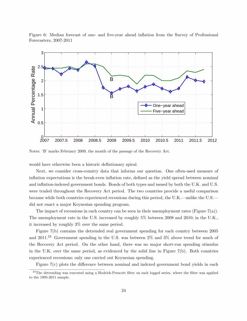
Figure 6: Median forecast of one- and five-year ahead inflation from the Survey of ProfessionalForecasters, 2007-2011
2007 2007.5 2008 2008.5 2009 2009.5 2010 2010.5 2011 2011.5 20120
0.5
1
1.5
2
2.5
3
Ann
ual P
erce
ntag
e R
ate
B
B
One−year aheadFive−year ahead
Notes: ‘B’ marks February 2009, the month of the passage of the Recovery Act.
would have otherwise been a historic deflationary spiral.
Next, we consider cross-country data that informs our question. One often-used measure of
inflation expectations is the break-even inflation rate, defined as the yield spread between nominal
and inflation-indexed government bonds. Bonds of both types and issued by both the U.K. and U.S.
were traded throughout the Recovery Act period. The two countries provide a useful comparison
because while both countries experienced recessions during this period, the U.K.—unlike the U.S.—
did not enact a major Keynesian spending program.
The impact of recessions in each country can be seen in their unemployment rates (Figure 7(a)).
The unemployment rate in the U.S. increased by roughly 5% between 2008 and 2010; in the U.K.,
it increased by roughly 3% over the same period.
Figure 7(b) contains the detrended real government spending for each country between 2005
and 2011.23 Government spending in the U.S. was between 2% and 3% above trend for much of
the Recovery Act period. On the other hand, there was no major short-run spending stimulus
in the U.K. over the same period, as evidenced by the solid line in Figure 7(b). Both countries
experienced recessions; only one carried out Keynesian spending.
Figure 7(c) plots the difference between nominal and indexed government bond yields in each
23The detrending was executed using a Hodrick-Prescott filter on each logged series, where the filter was appliedto the 1995-2011 sample.
24

Figure 7: Unemployment, government spending and expected inflation in the U.S. and U.K., 2005-2011
2005 2006 2007 2008 2009 2010 20114
5
6
7
8
9
10
Per
cent
(a) Unemployment rate
United StatesUnited Kingdom
2005 2006 2007 2008 2009 2010 2011−2
−1
0
1
2
3
Per
cent
age
devi
atio
n
(b) Real government expenditure
United StatesUnited Kingdom
2005 2006 2007 2008 2009 2010 2011−2
−1
0
1
2
3
4
Ann
ual P
erce
ntag
e R
ate
(c) Expected inflation (nominal−indexed yield spreads)
United StatesUnited Kingdom
Note: Government spending is deviation of log spending from an Hodrick-Prescott trend.
25

country. This difference is the break-even inflation rate, which is often used to measure expected
inflation. Consider the break-even inflation rate in the U.S (the diamond-labeled line). From the
beginning of through the fall of 2008, break-even inflation in the U.S. fell from roughly 2.5% to -1.5%.
This is consistent with the market participants forecasting a decline in the price level. During the
three months that followed, roughly following the Democrat presidential and congressional victories,
U.S. break-even inflation increased by roughly 2%. Considered in isolation, this is qualitatively
consistent with the expected inflation channel. That is, the political wins signaled news of an
upcoming Keynesian stimulus, which bid up the expected future real wage relative to a no-stimulus
baseline. In turn, increased marginal cost would cause future nominal price increases.
However, in the U.K. there was a similar increase in expected inflation over the same three
months, despite the fact that the U.K. had no substantial short-run spending stimulus. The British
government’s primary anti-recession instrument was a temporary reduction in the value-added tax
rate. It took effect through the Value Added Tax (Change of Rate) Order in December 2008 and
was then extended as part of the Finance Act 2009. The Finance Act 2009 included only a few
spending programs, such as £1B to support the green-energy sector.
The U.K. experience is counterevidence to a strong expected inflation channel in the U.S. Had
the U.S. expected inflation increase been driven by the Recovery Act, then the channel suggests
that the U.K. should have entered a deflationary spiral following the absence of a British Keynesian
stimulus.
Next, we explain why the jump in U.S. break-even inflation seen in Figure 7(c) was more likely
due to another factor rather than news of the Recovery Act.24 First, the major decrease and then
increase of the U.S. nominal-indexed yield spread in 2008 came largely from a rise and then decline
in the yield on indexed bonds. Figure 8 plots the daily yield on that bond from September through
December of 2008.
The rise in this yield occurred over a period of several months; however, most of the decline
in that yield, and most of the rise in break-even inflation, occurred within a 3 trading day time
span: Wednesday, November 26 to Monday, December 1.25 On November 26, the Federal Reserve
announced its plans to buy $800 billion worth of mortgage-backed securities. December 1 marked
Federal Reserve Chairman Ben Bernanke’s speech to the Austin Chamber of Commerce, outlining
his commitment to continued monetary easing. This included a commitment to continued large-
scale asset purchases along with further federal funds rate cuts.
The dramatic decline in the indexed bond yield aligns to the day with an historic unconventional
monetary policy announcement. This leads us to ask whether any fiscal policy announcements
preceding the Recovery Act aligned with major changes in break-even inflation.
24See Neely (2010) for a further discussion of the issue.25Thanksgiving landed on November 27 of that year.
26

Figure 8: Daily yield on constant-maturity, five-year U.S. Treasury inflation-indexed bonds
9/23/08 10/7/08 10/22/08 11/5/08 11/20/08 12/5/08 12/19/081
1.5
2
2.5
3
3.5
4
4.5
Yie
ld (
%)
Fed chairman describes credit−easing plan, 12/1 →
$800B LSAP plan announced, 11/26 →
Notes: LSAP stands for “large scale asset purchases”.
3.3 Isolating the Spending Shock using Fiscal Policy Announcements
The November 26, 2008 Large Scale Asset Purchase announcement provided one instance where an
interest rate has moved dramatically at the time of an announcement about monetary/credit policy.
This movement implied a large change in break-even inflation, which is sometimes interpreted as a
change in inflation expectations. Along the same line of argument, if the expected inflation channel
of fiscal policy were operative and quantitatively important one might predict that upward jumps
in break-even inflation would occur at the time of expansionary fiscal policy news. We investigate
this possibility for the Recovery Act period.
To accomplish this, we examined newspaper articles, position papers and political speeches—
recording the particular calendar dates that this information became available to the public. This
narrative approach delivered eight distinct key news events between October 12, 2008 and February
18, 2009. These are presented in Table 6. The October 12 news was the release of then-candidates
Barack Obama and Joe Biden’s “Rescue Plan for the Middle Class.” That plan was estimated to
cost $175 billion. Examples of other events include: Obama’s presidential victory and major gains
in Congress on November 3, Obama’s announcement of the first details of his Recovery Plan on
December 6, and the Senate passage of the Recovery Act on February 10.
Next, we calculate the daily break-even inflation rate using the 5 year maturity bonds. By
examining daily data, we are likely able to distinguish these announcements about fiscal policy
27

Table 6: Significant fiscal policy news announcements preceding the 2009 Recovery Act
Event Date 2008
(A) Then-candidates Obama and Biden release “A Rescue Plan for the Middle Class,” a stimulus plan estimated to cost $175 billion
Oct. 12
(B) First newspaper reports that congressional Democrats planning to introduce stimulus plan costing $300 billion.
Oct. 14
(C) Obama wins presidency, Democrats achieve major gains in Congress
Nov. 4
(D) Obama gives address calling for decisive government action including putting 2 million people to work rebuilding roads, bridges and schools
Nov. 15
(E) Senator Charles Schumer, Joint Economic Committee Chair, states that stimulus would need to be between $500 and $700 billion
Nov. 23
(F) Obama announces first details of his recovery plan, including some general categories
Dec. 6
2009 (G) U.S. Senate approves the Recovery Act Feb. 10 (H) Obama signs the Recovery Act into law Feb. 18
from other shocks hitting the economy. Figure 9 plots the break-even inflation rate (APR) time
path for each of the eight events. Each event corresponds to one line, marking the three (calendar)
days before through three days after the event. A break in a particular line occurs when the
corresponding time interval includes one or more non-trading days.
For all but one of the eight events, break-even inflation moves by less than 25 basis points from
before to after announcement. At the time of Nov. 23 event, the Senate Joint Economic Committee
Chair’s announcement that a $500 to $700 billion stimulus would be necessary, break-even inflation
increased 104 basis points.
3.4 Isolating the Spending Shock using Professional Forecasts
The 2008-2009 path of the median value of professional forecasters’ expected inflation presented
earlier should be interpreted with caution because events other than spending changes may have
influenced these forecasters’ expectations. For example, one could imagine that news of the forth-
coming Act (by itself) did substantially increase median inflation expectations, while over that
same time frame, other “offsetting” news arrived that substantially decreased median inflation ex-
pectations. Together these two pieces of news might have summed to the observed small decrease
in the quarter-to-quarter survey responses.
With this concern in mind, we next control for the aggregate time-specific factors that may have
28

Figure 9: Break-even inflation rates (APR) in windows surrounding significant fiscal policy newsannouncements
‐4.0
‐3.0
‐2.0
‐1.0
0.0
1.0
2.0
3.0
4.0
‐4 ‐3 ‐2 ‐1 0 1 2 3 4
Oct. 12
Oct. 14
Nov. 4
Nov. 15
Nov. 23
Dec. 6
Feb. 10
Feb. 18
Calendar days since fiscal stimulus news
influenced the median forecast by examining the data at the individual forecaster level. The panel
consists of 22 forecasters, each of whom completed surveys in 2008:Q3, 2008:Q4 and 2009:Q1 and
whose responses included forecasts of federal government spending, total employment and inflation
expectations.
According to the expected inflation channel, when one of the respondents began predicting a
stimulus, then that respondent ought to simultaneously increase her inflation expectations. Some
notation is useful here. Let ft,j (x) = Ejt (xt+4)−Ej
t−1 (xt+3) where Ejt denotes the expectation of
forecaster j at time t. x is a random variable that may or may not take a time index.
Table 7 reports ft,j (π) and ft,j(gGOV
),i.e. the change in the forecast, from one quarter to
the next, of (i)one-year expected inflation, and (ii) the 1 year-ahead growth rate of real federal
expenditures.26
Each column corresponds to the survey quarter. Each row corresponds to a forecaster; for each
forecaster, numbers set in bold reflect the quarter at which the forecaster has the largest increase
in her spending growth forecast.
Consider, for example, Forecaster 2. Forecaster 2 reported an increase in 1-year-ahead expected
government spending growth of 9.3% in the 2008:Q4 survey. In the following quarter, Forecaster 2
predicted a modest 1.5% increase in her forecast of government spending growth. We interpret the
9.3% increase as reflecting the forecaster responding to news of a potential, upcoming Keynesian
stimulus. Examining the table, Forecaster 2 increased her inflation expectations in 2008:Q4 by only
26To conserve space, we exclude from the table the respondents who reported very little change in governmentspending expectation.
29

Table 7: Change in forecasts of 1-year-ahead inflation and of 1-year-ahead federal governmentspending growth, by forecaster
t=2008:Q4 t=2009:Q1 t=2009:Q2
Gov. Gov. Gov.Forecaster j spending Inflation spending Inflation spending Inflation
1 0.4 -0.5 13.1 -0.6 -2.9 0.02 9.3 0.2 1.5 -0.7 -1.9 0.13 1.4 1.1 8.4 -0.1 0.0 -0.24 0.2 0.6 4.3 -1.2 0.3 -0.35 0.9 -0.5 4.2 -1.8 -1.8 1.16 3.8 0.1 3.7 0.3 1.2 -0.27 -0.2 -1.1 2.0 0.0 3.8 -0.08 2.0 0.3 3.8 0.6 0.4 -0.49 0.8 -0.6 3.3 -0.3 -1.8 0.210 2.9 0.1 0.2 -2.8 -0.7 2.211 -0.0 -2.1 1.8 -0.7 2.9 0.612 -0.8 0.6 -0.4 0.2 2.7 -0.713 0.4 0.2 2.3 0.0 -0.9 1.114 1.9 -0.7 -0.4 0.5 1.0 -2.015 1.7 0.4 1.0 -0.7 -0.6 -0.2
Notes: Government spending column values are Ejt (gGov
t+4 ) − Ejt−1(gGov
t+3 ), where j denotes the forecaster.
Inflation column values are Ejt (πt+4) − Ej
t−1(πt+3). Values in bold indicate the time associated with the
largest change in the forecast of government spending growth, by forecaster. The table excludes forecasters
with very small changes in their forecasts of government spending growth.
30

Table 8: Estimates of response of innovation to 1-year-ahead inflation forecast with respect to a 1percent positive innovation to expected government spending growth forecast
Cross Section Panel Survey quarter(s) used
2008:Q4
(i)
Forecaster largest response quarter
(ii)
2008:Q3, 2008:Q4, 2009:Q1
(iii) Forecast innovation to Δ gov. spending
-0.012 (0.054)
0.029 (0.050)
-0.011 (0.043)
90% CI [-0.125, 0.100] [-0.076, 0.133] [-0.098, 0.075] Time fixed effects? No No Yes R2 0.002 0.010 0.104
Note: Data are from the SPF.
20 basis points relative to the previous quarter.
Examining Table 7, we see that 12 of the forecasters predicted large increases (at least 2.5%)
from one survey quarter to the next in the annual growth rate of government spending. There
was dispersion across forecasters in both the timing and the magnitude of their projected spending
increases; however, none of these increases was associated with large increases in expected inflation.
The largest increase in expected inflation at one of these spikes was 60 basis points.
Next, we run regressions using this forecaster-level data. Our first specification is
ft,j (π) = a+ b× ft,j(gGOV
)+ εt,j
Column (i) of Table 8 reports b when the forecast quarter is 2008:Q4. This is the quarter when
the Democrats won the White House and Congress, making a federal spending program much
more likely. The point estimate is -0.012, which means that a 1 percent positive innovation to a
forecaster’s expected government spending over the following year was associated with a 1.2 basis
point reduction in her 1-year-ahead inflation forecast. The response is not statistically different
from zero.
Column (ii) uses the same regression with one exception. Rather than choosing the same forecast
quarter for each forecaster, the time index for each forecaster is chosen based on each forecaster’s
largest spending innovation, (i.e. the bold-faced numbers in Table 7).27
The point estimate is 0.029. This means that a 1% unanticipated increase in expected gov-
ernment spending growth is associated with a 2.9 basis point increase in expected inflation. The
27The sample also includes the data for the seven forecasters not included in the table.
31

coefficient is not statistically different from zero.
Since the Recovery Act constituted a roughly 3.3% increase in government spending (each
year for three years), the point estimate suggests that the Act was associated with an 8.7 basis
point (= 3.3 × 2.9 basis points) increase in expected inflation. The 90% confidence interval for
this elasticity is (-0.08%, +0.13%). Using the upper bound of this confidence interval, a spending
increase with a magnitude of the Recovery Act would be associated with an increase in expected
inflation of 43 basis points.28
Column (iii) reports the estimated response when the entire panel is used and we include time
fixed effects. The results are similar to the two cross-sectional specifications. Thus, both the panel
and cross-sectional estimates imply we can reject a large expected inflation response to the Act.
4 Existing Research in the Context of Our Work
This section focuses on the existing work on this topic that is particularly relevant to our study.
First, Erceg and Linde (2012) document how the expected inflation channel can lead to a large
output multiplier, while simultaneously having minimal government budgetary costs when an econ-
omy is at the zero lower bound. They then ask why, given the effectiveness of these policies, do
policymakers limit the size of their spending programs under these circumstances? Their answer
is that the timing of the economy’s exit from a liquidity trap is endogenous. Moreover, at higher
spending levels, the economy endogenously leaves the liquidity trap sooner. In turn, this decreases
the size of the multiplier even when the economy is concurrently at the zero lower bound. Thus,
there are diminishing and possibly negative returns to larger and larger spending programs.
Our findings suggest a different answer to their question: the expected inflation channel is
quantitatively weak. Absent this mechanism, government spending is less likely to expand private
economic activity.
Also, Erceg and Linde (2010) note that expected inflation, measured from the median value of
the SPF, and actual inflation in the first two quarters following the passage of the Recovery Act
moved quantitatively much less than implied by the calibrated sticky price model (their Figures 5a
and 5b). We report this feature and also show that the pattern continues in the years following the
Act’s passage. We further show that the pattern is confirmed in a panel analysis of the professional
forecasters, as well as in a cross-country comparison of nominal-indexed bond yield spreads.
28Note that if we take the index ft,j forward one period, there is both a change in the conditioning information andalso a shift forward in the random variable by one quarter. If we wish to perfectly isolate the change in information,we could use a more sophisticated measure. For the inflation innovation, we would have
ft,j (Pt+3/Pt) = Ejt (Pt+3/Pt) − Ej
t−1 (Pt+3/Pt)
Using this measure would mean we would only be able to use 3-quarter-ahead, instead of our 4-quarter-ahead, inflationand spending growth measures. In results not presented here, we have shown that using ft,j (x) has negligible effectson our results.
32
Erceg and Linde (2012) explain how the size of the government spending multiplier, under
a nonresponsive monetary policy, can be tied closely to the duration of price contracts. In one
illustrative calibration (their Figure 3), they show how the output multiplier can be slightly greater
than 1 under 10-quarter contracts and 25 under 10-quarter contracts. This is consistent with our
analysis that a high output multiplier goes hand in hand with a large inflation response.29
In their calibrated medium-scale sticky price model (similar to that of Christiano, et.al. (2005)),
Erceg and Linde (2012) find a muted response of inflation to a government spending shock—there
is a roughly 20-basis-point inflation rate in the first year following an AR(1) spending shock with a
cumulative value equal to 2.5% of one year of steady-state government spending (the dash-dotted
line in their Figure 5). The corresponding impact multiplier is roughly 1 and their cumulative
multiplier is approximately 0.5.30
Next, Davig and Leeper (2011) study government spending shocks in a sticky price model
under several different monetary/fiscal policy scenarios. They document how the expected inflation
channel (although they do not use that term) operates when monetary policy is passive, and not
simply at the zero lower bound. In contrast to Davig and Leeper (2011), our estimation of macro
responses to spending shocks under passive policies using a structural vector-autoregression does
not by itself depend on specifying a particular dynamic equilibrium model.
Next, whereas we find that the expected inflation channel was ineffective during the Recovery
Act episode, Eggertsson (2012) states that the New Deal was very effective in reversing the initial
contraction during the Great Depression. Following the line of reasoning offered in Eggertsson
(2012), we offer a rationale for why the New Deal might have “worked” whereas the Recovery Act
did not. First, the National Industrial Relations Act (NIRA) of 1933 gave goods market power to
large corporations and labor market power to unions, which would have directly exerted upward
pressure on markups and, therefore, inflation. In contrast, the Recovery Act expended a tremendous
dollar amount; however, it did less to influence the degree of market power in the economy. Thus,
the Recovery Act influenced prices more indirectly—through the government’s increased demand
for goods.
Several authors have noted that the channel is most effective when the government spending
ends as soon as monetary policy is no longer passive. Eggertsson (2012) explains that the NIRA
could be ended immediately either by the presidential proclamation or Congress. He interprets this
to mean that the emergency measures would last as long as the shock.
With respect to the Recovery Act, reversing the measures once they were enacted was infeasible.
In the first few months following the Act’s passage, the federal government obligated hundreds of
29Denes and Eggertsson (2009) and Woodford (2011) show that a much larger intertemporal elasticity of substitutionfor consumption, relative to those commonly used, can result in both a large output multiplier and a moderate inflationresponse. A higher intertemporal elasticity can generate a large consumption response, even if the real interest ratedecline is moderate as a result of a moderate increase in expected inflation. Their models are calibrated based ontheir analyses of the economic environment during the Great Depression rather than that for the post-WWII U.S.
30The multiplier increases somewhat when they add rule-of-thumb consumers and financial frictions.
33

billions of dollars to state and local governments, nonprofit organizations and transfer recipients
to be outlaid over the following several years. We contend that the federal government’s attempt
to renege on these commitments (supposing a fast economic recovery followed the Act’s passage)
would have created a political firestorm, and thus was unfeasible.
Our work is also related to several other papers on the expected inflation channel. First,
Cochrane (2013) suggest an alternative to the rational expectations equilibrium concept entitled
the “local-to-frictionless” equilibrium that undoes the large multiplier effect and several paradoxes
in this line of research. His paper provides one potential explanation for why we find a small
expected inflation effect in the post-WWII U.S. Second, Wieland (2013) shows that theoretically,
at the zero-lower bound, negative supply shocks can be expansionary but evidence (from oil supply
disruptions and earthquakes) is inconsistent with this phenomenon. Third, Bachman, Berg and
Sims (2013) examines household-level survey data to assess whether higher inflation expectations
lead to greater readiness to make a durable good purchase. They find that higher expected inflation
reduces a household self-reported likelihood of making the purchase.
5 Conclusion
We conclude by addressing economists’ state of understanding about the Recovery Act’s short-
term economic impact. Researchers have explored two distinct classes of mechanisms by which the
Act, and government stimulus spending more generally, can influence economic activity: through
a traditional mechanism and/or spillovers.
First, the traditional mechanism is that spending increases output and employment in the area
where that stimulus money is spent. According to the traditional Keynesian logic, government
purchases of furnish wages to workers, who in turn purchase goods that further stimulate output
and employment nearby. This traditional mechanism has been estimated using cross-state variation
in Recovery Act spending and economic outcomes. The preponderance of evidence from these
studies is either that there is no statistically significant effect of spending on employment or that
employment increases but at a very high price tag.31
The second class of mechanisms works through spillovers—output or employment goes up be-
cause of spending, but not because spending occurs nearby. The key difference between the spillover
mechanisms from the traditional mechanism is that the effect on economic activity can be unrelated
to the corresponding nearby spending.
The expected inflation channel is one such spillover mechanism that has been hypothesized.
Why is this channel a spillover mechanism? Greater government spending in Iowa has an effect
nationwide on expected inflation. This in itself will tend to increase consumption in Georgia
through a fall in the real interest rate, even if Georgia were to receive no stimulus dollars at all.
31See, for example, Conley and Dupor (2013), Dupor (2013), Wilson (2011) and Feyrer and Sacerdote (2012). Aclosely related paper is Dupor (2012).
34

This paper has provided evidence that this particular channel was quantitatively small during
the Recovery Act episode; other types of spillover mechanisms may have been more significant.
Consider taxes as one example. If Recovery Act spending signaled higher future tax rates,
especially on capital, then this could have reduced economic activity upon news/passage of the
Act. Exploring the magnitude by which higher expected future taxes rates might have reduced
private activity during the Recovery Act episode merits future research.
Next, interstate or interregional movements in goods or factors of production provide other
sources of spillovers. A negative spillover might occur if government spending in one state creates
job openings that draw workers from other states. A positive spillover might occur if government
spending in one state provides income to citizens of that state, who in turn buy goods from other
states.
References
American Recovery and Reinvestment Act, Public Law 111-5, 111th Congress, 17 Feb 2009.
Auerbach, A. and Y. Gorodnichenko (2012), “Measuring the Output Response to Fiscal Policy,”
American Economic Journal: Economic Policy 4, 1-17.
Bachman, R., T. Berg and E. Sims (2013), “Inflation Expectations and Readiness to Spend: Cross-
Sectional Evidence,” NBER Working Paper.
Bernstein, J. and C. Romer (2009), “The Job Impact of the American Recovery and Reinvestment
Plan,” Office of the Vice President-elect, working paper.
Blinder, A. and M. Zandi (2010), “How the Great Recession Was Brought to an End.”
Boivin, J. and M. Giannoni (2006), “Has Monetary Policy Become More Effective?” Review of
Economics and Statistics 88, 445-462.
Carlstrom, C., T. Fuerst and M. Paustian (2012), “Fiscal Multipliers Under an Interest Rate Peg
of Deterministic vs. Stochastic Duration,” Federal Reserve Bank of Cleveland, working paper.
Christiano, L. (2004), “The Zero-Bound, Zero-Inflation Targeting and Output Collapse,” North-
western University, manuscript.
Christiano, L., M. Eichenbaum and C. Evans (2005), “Nominal Rigidities and the Dynamic Effects
of a Shock to Monetary Policy,” Journal of Political Economy 113, 1-45.
Christiano, L., M. Eichenbaum and S. Rebelo (2011), “When Is the Government Spending Multi-
plier Large?” Journal of Political Economy 78-121.
35

Clarida, R., J. and M. Gertler (2000), “Monetary Policy Rules and Macroeconomic Stability:
Evidence and Some Theory,”Quarterly Journal of Economics.
Cochrane, J. (2013), “The New-Keynesian Liquidity Trap,” University of Chicago, working paper.
Conley, T. and B. Dupor (2013), “The American Recovery and Reinvestment Act: Solely a Gov-
ernment Jobs Program?” Journal of Monetary Economics, forthcoming.
Council of Economic Advisers (various quarterly reports), “The Economic Impact of the American
Recovery and Reinvestment Act of 2009.”
Davig, T. and E. Leeper (2011), “Monetary-Fiscal Policy Interactions and Fiscal Stimulus,” Euro-
pean Economic Review 55, 211-227.
Denes, M. and G. Eggertsson (2009), “A Bayseian Approach to Estimating Tax and Spending
Multipliers” Federal Reserve Bank of New York, working paper.
Dupor, B. (2012), “The 2009 Recovery Act: Directly Created and Saved Jobs Were Predominantly
in Government,” The Ohio State University.
Dupor, B. (2013), “Creating Jobs via the 2009 Recovery Act: State Medicaid Grants Compared to
Broadly-Directed Spending,” The Federal Reserve Bank of St. Louis.
Eggertsson, G. (2004), “Monetary and Fiscal Coordination in a Liquidity Trap,” Chap. 3 of “Op-
timal Monetary and Fiscal Policy in the Liquidity Trap,” PhD diss., Princeton Univ.
Eggertsson, G. (2012), “Was the New Deal Contractionary?” American Economic Review 102,
524-555.
Erceg, C. and J. Linde (2010) “Is There a Fiscal Free Lunch in a Liquidity Trap?” Board of
Governors of the Federal Reserve System, working paper.
Erceg, C. and J. Linde (2012), “Is There a Fiscal Free Lunch in a Liquidity Trap?” Board of
Governors of the Federal Reserve System, working paper.
Federal Reserve Bank of Philadelphia (2012),“Survey of Professional Forecasters: Documentation,”
updated August 10.
Feyrer, J. and B. Sacerdote (2012), “Did the Stimulus Stimulate? Effects of the American Recovery
and Reinvestment Act,” Dartmoth College, working paper.
Fisher, J. and R. Peters (2010), “Using Stock Returns to Identify Government Spending Shocks,”
Economic Journal 120, 414-36.
36

Neely, C. (2010), “The Effects of Large-Scale Asset Purchases on TIPS Inflation Expectations,”
Federal Reserve Bank of St. Louis National Economic Trends, September.
Ramey, V. (2011), “Identifying Government Spending Shocks: It’s All in the Timing,” Quarterly
Journal of Economics 126, 1-50.
Ramey, V. and M. Shapiro (1998), “Costly Capital Reallocatoin and the Effects of Government
Spending,” Carnegie-Rochester Conference Series on Public Policy, June
Summers, L. (2008), “Update on Economic Policy Work,” memo to President-Elect Obama, De-
cember 15.
Taylor, John (1999), “A Historical Analysis of Monetary Policy Rules,” in Monetary Policy Rules,
University of Chicago Press.
Taylor, John (2007), Getting Off Track, Hoover Press.
Wieland, J. (2013), “Are Negative Supply Shocks Expansionary at the Zero Lower Bound,” Uni-
versity of California–Berkeley, working paper.
Wilson, D. (2011), “Fiscal Spending Multipliers: Evidence from the 2009 American Recovery and
Reinvestment Act,” Federal Reserve Bank of San Fransico, working paper.
Woodford, M. (2011), “Simple Analytics of the Government Spending Multiplier,” American Eco-
nomic Association Journal: Macroeconomics 3, 1-35.
37