text mining for bioprocess identification fileabstract text mining, also referred to as text data...
TRANSCRIPT

FACULDADE DE ENGENHARIA DA UNIVERSIDADE DO PORTO
Text Mining for BioprocessIdentification
Pedro Couto
Mestrado Integrado em Engenharia Informática e Computação
Supervisor: Rui Camacho
July 27, 2018


Text Mining for Bioprocess Identification
Pedro Couto
Mestrado Integrado em Engenharia Informática e Computação
July 27, 2018


Abstract
Text Mining, also referred to as Text Data Mining, is the process of deriving high quality informa-tion and non-trivial patterns from text documents. It usually starts by transforming free-form textinto a more structured intermediate form, which will later be used to extract important knowledgeand patterns. Text Mining can be more complicated and complex than Data Mining due to thelack of structure and fuzziness inherent to text documents, since it is possible for text to carry thesame message in many different ways. This Information Extraction (IE) technique can be usedin many different areas, one of which is Biomedical Sciences. The volume of published researchmaterial is increasing rapidly, and so, the biomedical knowledge base is too. Besides, Text Miningis particularly difficult in this area due to the fact that many biological processes or concepts havedifferent designations and abbreviations, which makes it a real challenge to thoroughly analyze itall without overlooking something. Biomedical Text Mining (BTM) is the field that deals with theautomatic processing of biomedical literature and the retrieval of biomedical concepts. It coverstasks like Named Entity Recognition (NER), document classification and document summariza-tion, while also using knowledge from other fields like Machine Learning. It’s a promising andnecessary field, because it helps researchers deal with the information overload created by the ex-ponential growth of biomedical publications. The goal of this project is to review the state of theart, and explore the existing approaches to biomedical processes identification in order to come upwith a new one. We used life sciences text corpus available on the Web to assess the quality of thedeveloped tool. We performed several techniques such as Named Entity Recognition, Semanticand Syntactic Analysis, Word dependency, using tools like Genia Tagger, UMLS MetaMap andSpacy, and achieved a good level of identification of entities and biological events on a few corpusof text, as the case studies show.
i

ii

Resumo
Text Mining (Mineração de Texto), também conhecido como Text Data Mining (Mineração deDados de Texto), é o processo de derivar informação de alta qualidade e padrões não triviais apartir de documentos de texto. Começa-se normalmente por tranformar o texto em forma livrenuma representação intermédia mais estruturada, que será mais tarde usada para extrair conhec-imentos e padrões importantes. O Text Mining poderá ser mais difícil e complicado que o DataMining devido à falta de estrutura, confusão e imprecisão inerente aos textos, uma vez que épossível os textos exprimirem a mesma mensagem de várias maneiras diferentes. Esta técnicade extracção de conhecimento (Information Extraction - IE) pode ser usada em diversas áreas,sendo uma delas as Ciências Biomédicas. O volume de materiais de pesquisa a serem publicadostem aumentado exponencialmente, e consequentemente a base de dados biomédicos segue esteaumento. Para além disto, a Mineração de Dados nesta área é particularmente difícil nesta áreadevido ao facto de muitos dos processos e conceitos biológicos terem diferentes designações eabreviações, fazendo com que a análise destes documetos acabe por ser um enorme desafio, e quese torne dificil não deixar alguns detalhes escaparem. Biomedical Text Mining (BTM - Mineraçãode Textos Biomédicos) é a área que lida com o processamento automático de literatura biomédicaprocurando a aquisição de conceitos biomédicos. Engloba tarefas como Named Entity Recog-nition (NER - Reconhecimento de Entidades com Mencionadas), classificação e sumarização dedocumentos, usando também técnicas e conhecimentos de outras áreas como Machine Learning(Aprendizagem de Máquina). É uma área importante e com potêncial, uma vez que ajuda inves-tigadores e cientistas a lidar com a sobrecarga de informação criada pelo aumentos exponencialde publicações biomédicas. O objectivo deste projecto é fazer uma revisão ao estado da arte, eexplorar as abordagens existentes à identificação de processos biomédicos de modoa tentar desen-volver uma nova. Foram usados corpus de textos biomédicos disponiveis na Internet para avaliara qualidade da ferramenta desenvolvida. Foram executados vários processos como Named EntityRecognition, análise semântica e sintática, dependência de palavras através do uso de várias fer-ramentas, como Genia Tagger, UMLS MetaMap e SpaCy, e conseguimos atingir um bom nivelde identificação de entidades e processos biológicos em vários corpus de texto, tal como mostra oestudo.
iii

iv
Acknowledgements
To begin with, I want to thank my family, more precisely, my mother, my father and my brother foralways being there for me, and supporting me, not just during the development of this dissertation,but throughout my whole academic course.I would also like to thank my friends, for all the time we spent together. On one hand, we wereall going through the same, and it was easier to keep pushing through since we could all motivateone another, and on the other, for all the laughs and fun times we had to relieve the stress.A special thanks to my girlfriend, for always believing in me and helping me believe in myself.And finally, I would like to thank professor Rui Camacho, my supervisor, for all the support andguidance. I really could not have done this without him.
Pedro Couto
v

vi

“It is good to travel with hope and courage,but it’s better to travel with knowledge’
Ragnar Lothbrok
vii

viii

Contents
1 Introduction 11.1 Context and Motivation . . . . . . . . . . . . . . . . . . . . . . . . . . . . . . . 11.2 Structure . . . . . . . . . . . . . . . . . . . . . . . . . . . . . . . . . . . . . . . 2
2 Approaches to Text Mining 52.1 Bioprocesses . . . . . . . . . . . . . . . . . . . . . . . . . . . . . . . . . . . . 52.2 Text Mining . . . . . . . . . . . . . . . . . . . . . . . . . . . . . . . . . . . . . 6
2.2.1 Text Representation Schemes . . . . . . . . . . . . . . . . . . . . . . . 62.3 Text Analysis Stages . . . . . . . . . . . . . . . . . . . . . . . . . . . . . . . . 8
2.3.1 Text Preprocessing . . . . . . . . . . . . . . . . . . . . . . . . . . . . . 82.3.2 Classification . . . . . . . . . . . . . . . . . . . . . . . . . . . . . . . . 92.3.3 Random Forest . . . . . . . . . . . . . . . . . . . . . . . . . . . . . . . 102.3.4 Clustering . . . . . . . . . . . . . . . . . . . . . . . . . . . . . . . . . . 102.3.5 Information Extraction . . . . . . . . . . . . . . . . . . . . . . . . . . . 11
2.4 Tools for Text mining . . . . . . . . . . . . . . . . . . . . . . . . . . . . . . . . 122.4.1 GENIA Tagger . . . . . . . . . . . . . . . . . . . . . . . . . . . . . . . 122.4.2 SpaCy . . . . . . . . . . . . . . . . . . . . . . . . . . . . . . . . . . . . 132.4.3 UMLS . . . . . . . . . . . . . . . . . . . . . . . . . . . . . . . . . . . 14
2.5 Web Repositories of Life Sciences Literature . . . . . . . . . . . . . . . . . . . 142.6 Related Work . . . . . . . . . . . . . . . . . . . . . . . . . . . . . . . . . . . . 14
2.6.1 Turku Event Extraction System . . . . . . . . . . . . . . . . . . . . . . 142.7 Conclusion . . . . . . . . . . . . . . . . . . . . . . . . . . . . . . . . . . . . . 15
3 Information Extraction from Text Documents 173.1 Text Data . . . . . . . . . . . . . . . . . . . . . . . . . . . . . . . . . . . . . . 173.2 Text Processing . . . . . . . . . . . . . . . . . . . . . . . . . . . . . . . . . . . 213.3 Genia Tagger . . . . . . . . . . . . . . . . . . . . . . . . . . . . . . . . . . . . 223.4 UMLS MetaMap . . . . . . . . . . . . . . . . . . . . . . . . . . . . . . . . . . 243.5 SpaCy . . . . . . . . . . . . . . . . . . . . . . . . . . . . . . . . . . . . . . . . 253.6 OHSUMED Text Classification . . . . . . . . . . . . . . . . . . . . . . . . . . . 273.7 Chapter Summary . . . . . . . . . . . . . . . . . . . . . . . . . . . . . . . . . . 28
4 Case Studies 294.1 Genia Tagger . . . . . . . . . . . . . . . . . . . . . . . . . . . . . . . . . . . . 294.2 UMLS MetaMap . . . . . . . . . . . . . . . . . . . . . . . . . . . . . . . . . . 304.3 SpaCy + UMLS MetaMap . . . . . . . . . . . . . . . . . . . . . . . . . . . . . 304.4 Final Results . . . . . . . . . . . . . . . . . . . . . . . . . . . . . . . . . . . . 324.5 OHSUMED Corpus . . . . . . . . . . . . . . . . . . . . . . . . . . . . . . . . . 32
ix

CONTENTS
4.6 Chapter Summary . . . . . . . . . . . . . . . . . . . . . . . . . . . . . . . . . . 35
5 Conclusions 375.1 Accomplishments . . . . . . . . . . . . . . . . . . . . . . . . . . . . . . . . . . 375.2 Future Work . . . . . . . . . . . . . . . . . . . . . . . . . . . . . . . . . . . . . 38
References 41
A POS Tags 45
B UMLS Semantic Types and Groups 47
x

List of Figures
1.1 Genia event task example . . . . . . . . . . . . . . . . . . . . . . . . . . . . . . 2
2.1 Visualization of NERs with SpaCy . . . . . . . . . . . . . . . . . . . . . . . . . 132.2 Visualization of Word Dependencies with SpaCy . . . . . . . . . . . . . . . . . 132.3 TEES process representation . . . . . . . . . . . . . . . . . . . . . . . . . . . . 16
3.1 Text Processing Diagram . . . . . . . . . . . . . . . . . . . . . . . . . . . . . . 22
xi

LIST OF FIGURES
xii

List of Tables
2.1 Event types and their arguments for the BioNLP-ST Genia Event . . . . . . . . . 62.2 Genia Tagger training scores . . . . . . . . . . . . . . . . . . . . . . . . . . . . 13
4.1 Genia Tagger Performance . . . . . . . . . . . . . . . . . . . . . . . . . . . . . 304.2 Genia Tagger Total Score . . . . . . . . . . . . . . . . . . . . . . . . . . . . . . 304.3 UMLS MetaMap Performance . . . . . . . . . . . . . . . . . . . . . . . . . . . 314.4 UMLS MetaMap Total Score . . . . . . . . . . . . . . . . . . . . . . . . . . . . 314.5 SpaCy + UMLS MetaMap Performance . . . . . . . . . . . . . . . . . . . . . . 324.6 SpaCy + UMLS MetaMap Total Score . . . . . . . . . . . . . . . . . . . . . . . 324.7 Final Process Performance . . . . . . . . . . . . . . . . . . . . . . . . . . . . . 334.8 Final Process Total Score . . . . . . . . . . . . . . . . . . . . . . . . . . . . . . 334.9 J48 Classification Performance . . . . . . . . . . . . . . . . . . . . . . . . . . . 334.10 J48 Classification Performance with new Dataset . . . . . . . . . . . . . . . . . 344.11 Random Forest Classification Performance . . . . . . . . . . . . . . . . . . . . . 344.12 Random Forest Classification Performance with New Dataset . . . . . . . . . . . 344.13 SGD Classification Performance . . . . . . . . . . . . . . . . . . . . . . . . . . 344.14 SGD Classification Performance with new Dataset . . . . . . . . . . . . . . . . 344.15 IBk Classification Performance . . . . . . . . . . . . . . . . . . . . . . . . . . . 344.16 IBk Classification Performance with new Dataset . . . . . . . . . . . . . . . . . 34
xiii

LIST OF TABLES
xiv

Abbreviations
BioNLP-ST BioNLP Shared TaskBTM Biomedical Text MiningHMM Hidden Markov ModelsIE Information ExtractionIR Information RetrievalML Machine LearningNE Named EntityNER Named Entity RecognitionNLP Natural Language ProcessingPOST Part of Speech TaggingRE Relation ExtractionSVM Support Vector MachinesTEES Turku Event Extraction SystemTF-IDF Term Frequency - Inverse Document FrequencyTM Text MiningUMLS Unified Medical Language SystemVSM Vector Space Model
xv


Chapter 1
Introduction
With all the technological advances that we have been witnessing, information systems have also
had their share of evolution. We live in a time where information is available to everyone provided
by an Internet connection. This increase in information and its availability led to the creation of
methods to better acquire knowledge[GCP14]. Since there is an ever growing amount of material
to read from, people felt the necessity to create tools to acquire the information in faster and
more simple ways. To help us deal with this information overload, there is a process called Text
Mining. It is the automatic process of obtaining useful information from text documents. During
this process the text will be analyzed and transformed into more appropriate representations in
order to summarize and take meaning out of the words. Text Mining can be used with many
different purposes, such as summarizing e-mails, online comments, articles and newspapers etc.
however in this dissertation the interest is in using Text Mining in biomedical documents in order
to extract knowledge from them.
1.1 Context and Motivation
Like it was mentioned above, the amount of information and its availability have been increasing
rapidly, and the biomedical area is no exception. A big part of this growth can be blamed on the
Internet because of its reach and accessibility. Taking advantage of what this network has to offer,
online forums and communities directed to the most diverse fields started appearing, creating a
virtual place where people with the same interests could communicate, exchange opinions and
ideas, as well as share their work or other kinds of content. One of the communities that benefited
from this trend, was that of researchers and academic users, since it allowed them to study and
read published material more easily[Bor12]. In these last years, we have been witnessing a rapid
increase of published material in the biomedical sciences area, and as such, automatic information
extraction methods became almost essential in order to deal with all the information becoming
available. The amount of content to read from is so large, that it became unfeasible and ineffective
1

Introduction
for humans to do it without the help of machines[Jha12]. Moreover, facing the mentioned growth
(that is still occurring), new methods, or improvements to the existing ones are becoming a neces-
sity, and it is the goal of this dissertation to satisfy it. Besides the rapid increase in publications
in this area, the other reason for focusing in the biomedical sciences is that Text Mining becomes
particularly difficult in this field. This is because the typical Information Retrieval tools struggle
to deal with the particularities found in the biomedical literature, such as the lack of normalization
in biomedical documents. There are no strict rules about the representation of proteins or events,
which means there could be different ways of representing the same thing, there is the possibil-
ity of finding some names (genes, proteins, etc.) that are the same as common words of day to
day life, and we also have to deal with abbreviations[ZDFYC07]. Sharing the same goal of help-
ing the biomedical community deal with the retrieval/extraction of information from this growing
amount of documents, the BioNLP-Shared Task challenges the interested in coming up with new
solutions to these problems. In their own words, "The BioNLP Shared Task (BioNLP-ST) series
represents a community-wide trend in text-mining for biology toward fine-grained information
extraction (IE)"1. One of the tasks from this community, namely, the BioNLP-Shared Task Ge-
nia Event task "has been promoting development of fine-grained information extraction (IE) from
biomedical documents", and it is in the light of this event that we will conduct this dissertation,
with the ultimate goal of making it easier for researchers to acquire the knowledge from all these
documents[KKHRS15]. Figure 1.1 show an example of the kind of entities and relations to be
extracted from the text documents. We will try to develop a new approach or a new tool, that can
perform this information extraction more effective and efficiently.
Figure 1.1: Genia event task example
1.2 Structure
Chapter 2 will dive into the process of Text Mining. We will review the state of the art, presenting
the existing approaches and defining the different stages of the whole process, while also describ-
ing how the different tasks and methods that constitute Text Mining work, and how the text will
be transformed into different kinds of representations throughout the whole pipeline of processes.
In this chapter, we will also present some available tools that perform said tasks, and how they can
be used in the pipeline.
Chapter 3 will present the methodology, how the problem was approached, and which tools were
1http://2016.bionlp-st.org/tasks/ge4
2

Introduction
used and how they were used, providing some insight on how they work, as well as their role in
the pipeline.
In Chapter 4 we will present the results, both for the individual tools in order to evaluate their
individual performance, and for the process as a whole. This chapter will also include a discussion
on the results, in order to try to understand the reasons behind them, and what they might suggest.
Finally, the fifth and last Chapter 5, the Conclusion, will be a reflexion on the research and work
done. It will present what accomplishments were achieved, and later, an exploration of future
work options following the work of this dissertation
3

Introduction
4
Chapter 2
Approaches to Text Mining
In this chapter we can find a description on the whole Text Mining process. We will go through
the preparations needed to perform on the data to analyze, providing some insight on the possible
ways of treating free form text into other text representations schemes that allows machines to
"understand" the meaning of said texts. We will also go through the stages of Text Mining while
also listing some of the already existing tools that aim to help on this process. Finally, we will
provide a list of some of the online repositories where we can find articles and biomedical publi-
cations, which in the end, are the target of the Text Mining techniques we will be reviewing and
developing throughout this dissertation.
2.1 Bioprocesses
Bioprocesses, or biological events, which are the target of this work, are series of events or molecu-
lar functions occurring inside living organisms [KKHRS15]. In Table 2.1 we can see which events
need to be addressed in this task as well as their arguments. A "+" sign in front of an argument
means that there could be more than one argument for the same event. Bellow we will provide a
brief description of these biological events[Lei17].
• Gene-expression - Process by which information from a gene is used in the synthesis of a
functional gene product. These gene products are usually proteins.
• Transcription - Process in which a particular segment of DNA is copied into RNA by the
enzyme RNA polymerase. It is the first step in Gene-expression.
• Protein-catabolism - The breakdown of proteins into amino acids and simple derivative
compounds.
• Phosphorylation - Attachment of a phosphoryl group to a molecule. It is an important
process for protein function because it activates or deactivates many enzymes, regulating
their function
5

Approaches to Text Mining
• Localization - Process in which a cellular entity is transported or maintained in a specific
location.
• Binding - An attractive interaction between two or more molecules that results in a stable
association.
• Regulation - A wide range of processes that are used by cells to increase or decrease the
production of specific gene products
Table 2.1: Event types and their arguments for the BioNLP-ST Genia Event
Event Type Primary Argument Secondary ArgumentGene-expression Theme(Protein)Transcription Theme(Protein)Protein-catabolism Theme(Protein)Phosporylation Theme(Protein) Site(Entity)Localization Theme(Protein) AtLoc(Entity), ToLoc(Entity)Binding Theme(Protein)+ Site(Entity)+Regulation Theme(Protein/Event), Cause(Protein/Event) Site(Entity), CSite(Entity)Positive-regulation Theme(Protein/Event), Cause(Protein/Event) Site(Entity), CSite(Entity)Negative-regulation Theme(Protein/Event), Cause(Protein/Event) Site(Entity), CSite(Entity)
2.2 Text Mining
Text Mining, or Text Data Mining, is the process of extracting valuable information from text
data by combining techniques from NLP (Natural Language Processing) and Machine Learning
[HNP05]. It usually starts by processing the input text, transforming it into more structured repre-
sentations, which makes it easier for machines to analyze it. With the resulting structured data, the
goal is to try to derive patterns by modeling relations between the words, trying to create meaning.
Text Mining involves techniques like Part of Speech Tagging (POST), Named Entity Recognition
(NER) and Sentiment Analysis, which will be better understood further ahead.
2.2.1 Text Representation Schemes
Like it was mentioned already, during the process, the text to analyze will suffer some changes
due to the execution of some Natural Language Processing tasks. These tasks will decompose the
text so that a deeper understanding of the various words can be achieved. We will be describing
some of the more common text representation schemes used in Text Mining, as well as how they
can be useful.
• String of characters - This is the most common and general way of representing text data,
since it allows you to represent any language as a sequence of characters. It is not very
helpful in terms of analysis however, because it does not recognize words, only characters,
6

Approaches to Text Mining
and these characters include spaces and punctuation. This type of representation is common
since it is the most fit for human reading, but it is not very adequate for machines to under-
stand its meaning. What it allows though, is to count the character frequency, however, this
will not help much when the goal is to extract knowledge from the sentences.
• Bag of words - This representation is obtained by splitting a String through the space (’ ’)
character (ignoring punctuation), which will result in a group of words. It provides a deeper
understanding to the machine since words are the basic unit in human communication. It
can also be called sequence of words if the order is kept as it was. This "bag" by itself
is not too valuable, since it lacks grammatical and sentimental characteristics, but it opens
the door for more analysis possibilities, which we will see further ahead. Another feature
that usually follows the Bag of words representation is the term count, which means that
if a sentence has repeated words, the bag will simply have one copy of each word, while
indicating how many times it appears.
• N-Grams - With the bag of words, the spacial information of the sentences is completely
lost, which means that we cease to know the order of the words in the original sentences.
The N-Gram, works in a similar way as the Bag of words, however instead of storing every
word, it stores every group of N words. Given the sentence "John likes movies" as example,
with an N=2 (bigram), the resulting set of words would be: ["John likes", "likes movies"].
This way it is possible to keep some spatial information, which allows for a better analysis
of the whole sentences or documents. Moreover, probability is also used with this scheme in
order to obtain groups of words that are relevant and have meaning. This means that we can
use the probability of a word "B" showing up after a certain word "A" in order to access if
the two words together "A B", actually mean something, or if it is relevant to analyze them
together [Wal06].
• Vector Space Model - In this model, each document is represented as a multi-dimensional
vector, being that each coordinate (dimension) of the vector represents the weight of each
term (one or more words, for instance "New York" should be kept together). The weight is
commonly calculated using the TF-IDF (Term Frequency - Inverse Document Frequency)
score, which reflects an evened frequency of the term. It does not only count the frequency,
because that would not be the most appropriate since very common words would have too
high scores (words like "the" or "one"), so it uses the inverse frequency to lower the score
of such words and raise the score of more uncommon ones. Since the documents are repre-
sented as vectors, we can then use the distance or the angle between them to get an idea of
the similarity between documents, or how related they are [VSM].
• Word2vec - It works in a very similar way as the previous representation, however, the
Vector Space Model only related the documents in accordance to term frequency, it has no
syntactic or semantic type of relations. The word2vec is a more advanced vector representa-
tion of terms, that uses distributional hypothesis to create better relations between words or
7

Approaches to Text Mining
terms. This hypothesis hints that you can take meaning out of a word by its context or com-
pany (where the word appears).[Hua] For instance if in two different sentences, there are
two different words in the same position, there is a chance they are semantically or syntacti-
cally related. To demonstrate this we will use these two sentences: "I’m going on Monday",
and "I’m going on Thursday". In this example, the words "Monday" and "Thursday" appear
in the same "position", which hints they might be related or synonyms, which in this case
they are, since they are both days of the week.
2.3 Text Analysis Stages
This section aims to provide some insight on the various tasks that Text Mining depends on. It
will go through text pre-processing tasks, Classification, Clustering and Information Extraction
Algorithms.
2.3.1 Text Preprocessing
Preprocessing the text is a key component in Text Mining, and can be crucial to get the best results.
It transforms the input text in more adequate forms for the machine to better analyze it [HNP05].
We will be describing the most common text preprocessing tasks.
• Tokenization - This step can be reduced to splitting the text through the ’space’ characters,
dividing the sentences into words or terms. Like it was said before, words are the basic unit
of human communication, and as such they provide the best means of analysis. This will
result in a list of tokens (terms), that will be submitted to other tasks. Tokenization, in some
cases, can also delete irrelevant certain irrelevant characters such as punctuation.
• Filtering - In this stage, the goal is to delete irrelevant words, that present few to none
importance to the extraction of knowledge. It is usually the deletion of stop-words (words
without much meaning to the sentences, e.g. prepositions), however some other words with
little relevance can be removed too.
• Part of Speech Tagging - POST is the process of adding tags to the words that identify their
grammatic group (e.g. noun, verb). It is basically a grammatical analysis, that adds another
layer of information, which will better help future processes and analysis, since it allows the
machine to know whether the words are verbs, nouns, adjectives, etc.
• Lemmatization / Stemming - This is the process of reducing the words to their most basic
form, which is often achieved by removing prefixes and/or suffixes. It is usually required
that a Part of Speech tagging be executed, so that the machine can discover which is the
basic form of that word. It will, for example, reduce the verb conjugations to their infinite
form and the nouns and adjectives to their basic, single form, mainly, like mentioned before,
by removing prefixes and suffixes.
8

Approaches to Text Mining
2.3.2 Classification
Classification can be one of the goals of Text Mining. It stands on trying to assign categories that
better describe the type of document being analyzed. Thus, the goal of Classification is to assign
predetermined labels to the various documents in the set [DD16]. In order to assess the quality of
the Classification approach, the F-1 score is commonly used (F-1 or Precision and Recall). There
are different methods available to perform this kind of evaluation, and we will be reviewing some
of them.
2.3.2.1 Naive Bayes
The Naive Bayes method is a probabilistic approach to classification. It is one of the most simple
classifiers as well as one of the most widely used. It is called Naive, because it makes the assump-
tion that all terms’ distribution is independent, which in most cases is obviously not true, however,
despite this assumption, the Naive Bayes Classifier performs notably well [HNP05]. It uses the
Bayes Rule to calculate the probability of a document belonging to a certain label, repeating the
process for all labels, and finally choosing the label with the highest probability. There are three
probabilities needed for this method: the probability of class Y happening, the probability of ob-
ject X happening in class Y, and the probability of object X happening. The final probability value
is calculated like shown:
P[Y |X ] =P[X |Y ] P[Y ]
P[X ]
This method is so popular, mainly because it is fast and accurate.
2.3.2.2 Nearest Neighbor
This method tries to assign a label taking into account the distance between said document, and
the documents from the different labels. It is a proximity based approach, in which this proximity
can be calculated through different ways, and one of these ways, is the distance or angle between
vectors, like we have seen in Vector Space Model and word2vec (visit 2.1.1). As such, the label
whose documents are the nearest to the document being analyzed, is the label that said document
would be assigned to [CH67]. This approach stands on the premise that the closer a document is
to each other, the more likely they are to be related. As such the each document will be assigned
to the label with the most close documents.
2.3.2.3 Decision Tree
Like the name indicates, this method uses a decision tree to assign a label to the document. In
this decision tree, each node represent an attribute, which the document may or may not have,
and the edges represent the "decision", in other words, the presence or absence of said attribute
[HNP05]. In a text domain, these attributes are most likely to be terms, and the decisions will be
made in accordance to the presence or absence of such terms. The document will then start at the
9

Approaches to Text Mining
root node, and it will work its way down until it reaches a leaf node which will reflect which label
must be assigned to it. The taller the decision tree, the more complex it will be, and expectantly
the better the results.
2.3.3 Random Forest
This algorithm can be used in Classification and Regression, and works as a large collection of
Decision Trees. It starts by dividing the sample set, containing all training data, into a random
number of various subsets, each containing a different combination of objects from the original
set. Then, for each subset, it will create a Decision Tree, hence the name Random Forest, due the
the random number of Decision Trees it creates. When classifying an object, each tree will output
its result, or its classification, and the final class it will return, is the class that was returned more
often by all the Decision Trees. Basically the different Decision Trees vote for a final Classification
[Bre01].
2.3.3.1 Support Vector Machines
SVM is a linear classifier, which means that the Classification decision will be made based on the
linear combination of the document’s features. Basically, an hyperplane is defined which separates
the 2 classes or labels. This hyperplane should be calculated in a way that it maximizes the margin,
or distance between the two classes. If it is not possible to define an hyperplane that completely
separates both classes, then an hyperplane is determined so that the least number of objects ends
up in the wrong side [LdC07]. This approach can only be used to classify an object between two
classes, but it presents very good results, and another good feature about this approach is that even
with high dimensional features, the method maintains a good performance.
2.3.4 Clustering
Clustering is a very popular Data Mining algorithm that has been used extensively in the text
domain. It provides functionalities in the range of classification and data visualization. What it
does is divide the documents in groups or clusters by similarity, so that similar documents end up in
the same group. This similarity is calculated using similarity functions, that can vary depending on
the clustering method in use [LA99]. Clustering can be performed with different granularities, in
a way that the analysis can be performed at different levels, that is so that the comparing factor can
be the whole document, paragraphs or even terms. There are many methods inside this category,
and we will be describing the most common ones.
2.3.4.1 Hierarchical Clustering
The name Hierarchical clustering is due to the way the clusters are organized after they have
been clustered using these algorithms, which can be compared to a tree. There are two types of
hierarchical clustering, top-down or divisive, and bottom-up or agglomerative. In the top-down
10

Approaches to Text Mining
approach, all the clusters are in the same group, being consecutively divided into sub clusters
as new conditions are added. In the bottom-up approach, all the documents are separated in the
beginning, and they start to group up into clusters, until in the end there is one super cluster with all
of them. To make the comparisons that originate the clusters, a distance method is used (similar to
vector space model). In the agglomerative approach, there are three merging techniques [HNP05].
1. Single Linkage Clustering - The two most similar documents are used as criteria.
2. Group Average Linkage Clustering - An average of the groups similarity is used as crite-
ria.
3. Complete Linkage Clustering - The least similar documents from 2 groups are used as
criteria.
2.3.4.2 K-means Clustering
This approach divides a group of documents into k clusters. It can be hard to find a good number
k of clusters, so it is also common to use an algorithm to find the best k. This process of finding
k is also referred as Seed Selection, and it can be accomplished using different methods (e.g.
random, buckshot) [LA99]. A simple approach to this type of clustering is, defining k data points
and calculate the distance between each document and those data points. The cluster to which
the document is assigned is the one that is the closest. In some cases, there is also a threshold
of similarity, which means that if a document is not similar enough to any cluster it will not be
assigned to any cluster.
2.3.5 Information Extraction
Information Extraction (IE) is the process or task of extracting useful information from text. This
text can be unstructured, which makes the process harder, or this same text could undergo some
preprocessing tasks beforehand [CL96], like the ones we mentioned earlier, in order to make it
easier to extract knowledge. This process has many applications in Biomedical Text Mining, and
that is why it is the most important in the context of this dissertation. Classifying or Clustering
documents is not really the the area we are trying to improve, but knowledge extraction is. We
will be describing some of the most common and important tasks of IE ahead.
2.3.5.1 Named Entity Recognition
During this process the group of terms will be tagged similarly to the POST process. However, in-
stead of just performing a grammatical analysis, this more sophisticated process will be identifying
the terms in accordance to a certain domain. For that, the task will be provided with dictionaries
and/or ontologies, with whom it may make comparisons to discover more about the word. This
way, it is possible to discover the meaning of the term, and find out if the term is the name of
a person, a city, or whatever it represents in its domain [Sil14]. It basically recognizes what the
11
Approaches to Text Mining
term actually is. That is why it is important to provide a good ontology so the results can be more
accurate. For instance, given a domain about historic buildings, this process could recognize the
term "Big Ben" as the British clock tower, however, if the specific ontology was not provided,
there could be a chance that the task would simply recognize the term as a person.
2.3.5.2 Hidden Markov Models
Hidden Markov Models (HMM), are probabilistic models that are vastly used for instance in the
Named Entity Recognition task. They differ from regular probabilistic models because, unlike
them, HMM take into account the neighbor results [HNP05]. In other words, when assigning
labels or tags to the terms, the Hidden Markov Models will consider one or some previously
assigned labels to help determine the current label, using the probability of such label appearing
after the previous ones. HMM can be represented as finite state automatons, where each state
represents a word and the transitions represent the probabilities of said words appearing after the
word in the current state. This model stands on two assumptions [Blu04]:
• Markov Assumption - The current state is dependent only on the previous state.
• Independence Assumption - The output observation at a certain time is dependent only
on the current state and independent from previous observations and states.
2.3.5.3 Relation Extraction
Relation Extraction (RE) is the task of discovering the semantic relation between terms in a text
[CR10]. These entities are previously discovered using methods like NER, and through RE, an
attempt is made to discover the relation between them [RE09]. The extraction is usually made at a
sentence level. To perform this kind of task, the most common types of methods are Classification
algorithms.
2.4 Tools for Text mining
2.4.1 GENIA Tagger
This tool encompasses most of the text preprocessing tasks discussed previously. It is able to
analyze text data written in English, and perform task like Stemming and Lemmatization, Part
of Speech Tagging and Named Entity Recognition. Besides, a good benefit from this tool is that
it is specifically tuned for biomedical literature, so it is adequate for extracting knowledge from
documents in this field [gen], and relevant to this dissertation. The tool was trained using the
NLPBA data set, and Table 2.2 1 shows the evaluation results for that performance.
1http://www.nactem.ac.uk/GENIA/tagger/
12

Approaches to Text Mining
Table 2.2: Genia Tagger training scores
Entity type Recall Precision F-scoreProtein 81.41 65.82 72.79DNA 66.76 65.64 66.20RNA 68.64 60.45 64.29Cell Line 59.60 56.12 57.81Cell Type 70.54 78.51 74.31Overall 75.78 67.45 71.37
2.4.2 SpaCy
SpaCy is an "industrial strength natural language processing tool"2. It is very complete performing
not only most of the text preprocessing tasks, but going further into some relation extraction and
dependencies modeling. It performs tasks like tokenization, Named Entity Recognition, Part of
Speech tagging, labeled dependency tagging, works in more than 27 languages and it is a fast and
robust platform, trusted by big companies like Airbnb and Quora [spa].
The Named Entity Recognition performed by this tool will not be relevant to this work since it was
not trained to deal with biomedical literature. As such, it recognizes more general purpose NEs,
like organizations and Geopolitical Entities. Another feature SpaCy provides is a visualizer, with
which it is possible to get a visual representation of the relations between words as well as the NEs
it recognizes. Figure 2.1 show the visualization of general purpose Named Entities, not relevant
for the Biomedical Sciences, and Figure 2.2 show the visualization of the word dependencies
extracted by SpaCy using the same sentence 3.
Figure 2.1: Visualization of NERs with SpaCy
Figure 2.2: Visualization of Word Dependencies with SpaCy
2https://spacy.io/3https://spacy.io/usage/spacy-101
13

Approaches to Text Mining
2.4.3 UMLS
Provided by the National Library of Medicine, "The UMLS, or Unified Medical Language Sys-
tem, is a set of files and software that brings together many health and biomedical vocabularies and
standards to enable interoperability between computer systems". It provides terms and codes and
the relations between them, from drugs to medical terms, as well as some Natural Language Pro-
cessing tools. There are two tools worth mentioning in the light of this dissertation: the first is the
Metathesaurus, which is "the biggest component of the UMLS. It is a large biomedical thesaurus
that is organized by concept, or meaning, and it links similar names for the same concept from
nearly 200 different vocabularies. The Metathesaurus also identifies useful relationships between
concepts and preserves the meanings, concept names, and relationships from each vocabulary"4.
The second is the UMLS Metamap, that maps concepts and terms from biomedical texts to the
UMLS Metathesaurus.
2.5 Web Repositories of Life Sciences Literature
The main online knowledge base revolves around the National Library of Medicine (NLM). They
provide us with the aforementioned UMLS (Unified Medical Language Systems), which is a
huge knowledge resource in this field, that integrates the vocabulary from the main biomedical
databases, while also providing a semantic network of medical terms and their relations. Also
provided by NLM we have MEDLINE, a huge database of bibliographic data providing journal
citations and abstracts from articles in the biomedical field, and PubMed, a search engine for
MEDLINE.
Apart from the NLM, there is also the BioNLP Shared Task, which besides challenging everyone
with these tasks and contests aiming to improve the Biomedical Text Mining approaches, also
provide the contestants with biomedical documents, some of them with the expected results after
performing the Text Mining process, i.e. denotations, to better help the users test and compete in
their challenges.
2.6 Related Work
The BioNLP-ST has been around for some years, and has had multiple editions. Since then, many
solutions and projects were developed in the light of this competition, and in this sections we will
be reviewing one of those solutions that really stands out from the others.
2.6.1 Turku Event Extraction System
"Turku Event Extraction System (TEES) is a free and open source natural language processing
system developed for the extraction of events and relations from biomedical text. It is written
4https://www.nlm.nih.gov/research/umls/knowledge_sources/metathesaurus/
14

Approaches to Text Mining
mostly in Python, and should work in generic Unix/Linux environments." 5 [Bjö14] This system,
from the Universirty of Turku started being developed in light of the BioNLP-ST 2009 edition. It
finished in first place, and kept being improved throughout the years. Besides winning in 2009, it
kept competing, entering in the 2011 and 2013 edition, finishing in first place in both of them as
well. Furthermore, it entered two editions of the DDI (Drug-Drug Interactions), having finished
in fourth place in 2011 and getting second and third place in 2013.
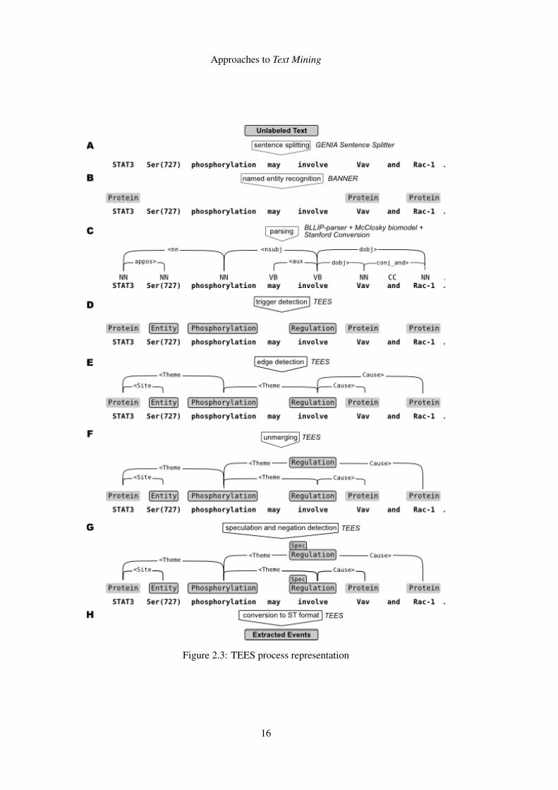
It uses known tools to perform syntactical analysis, text pre-processing and NER, such as GENIA
Sentence Splitter and BANNER. These tools are part of the first step of the system, and are used
to extract entities from the text. Later the system looks for trigger words, like verbs, to detect
relations and interactions. After this, complex events can be constructed and modifiers detected.
The result, will be a set of events returned in the Interaction XML format 6.
The main concept behind TEES’s ability to extract relations and events is a graph representation
for both syntactic and semantic information. In Figure 2.37 we have a visual representation of the
TEES process.
2.7 Conclusion
After reviewing the methods and tasks that constitute Text Mining, and going through some of the
available tools, it is possible to have a more profound understanding of the matter. This allowed
us to know how everything works, the stages the process has to go through, and how they connect,
as well as what tools we can use to perform them.
5https://github.com/jbjorne/TEES6https://github.com/jbjorne/TEES/wiki/Interaction-XML7https://github.com/jbjorne/TEES/wiki/TEES-Overview
15
Approaches to Text Mining
Figure 2.3: TEES process representation
16

Chapter 3
Information Extraction from TextDocuments
In this chapter we will describe our solution. We will start by showing the type of files to be
analyzed, i.e. its structure and contents, in order to shed some light on what kind of tasks might
be required to perform and how its contents will be used in the process. Then we will describe the
process itself, which tools were used, how they were used and what purposes they served, while
showing how the text was transformed.
3.1 Text Data
The text files used to develop our new approach in Biomedical Text Mining, are provided by the
BioNLP-ST 1. Participants of this task are provided with data sets composed of 776 JSON files
with annotated text. These denotations are the terms and expressions that are expected to be found
by the tool, and throughout all these files there is a total of 18694 denotations. Listing 3.1 shows
an example of one such file. Parts of the file were omitted to save space.
1 {
2 "target":"http://pubannotation.org/docs/sourcedb/PMC/sourceid
/1134658/divs/4",
3 "sourcedb":"PMC",
4 "sourceid":"1134658",
5 "divid":4,
1http://2016.bionlp-st.org/tasks/ge4
17

Information Extraction from Text Documents
6 "text":"Human B cells express BMP-6 receptors\nDetailed knowledge
regarding expression of different BMP receptors in B cells is
currently not available. To further elucidate the role of BMPs in
human B cells, we performed western blot analysis for type I and
type II BMP receptors. This analysis revealed that the type I
receptors Act-RIA, BMP-RIB and the type II receptors BMP-RII and
Act-RIIb are expressed on resting human B-cells (Figure 4). Ramos
cells expressed the type I receptors Act-RIA, weakly BMP-RIB and
the type II receptor BMP-RII, but more weakly than normal B
cells (Figure 4). HL60 cells were used for comparison and weakly
expressed Act-RIA and BMP-RII.\nTaken together, these data show
that normal human B cells and Ramos cells express a set of BMP
receptors, previously shown to bind BMP-6 [16].",
7 "project":"bionlp-st-ge-2016-reference",
8 "denotations":[
9 {
10 "id":"T1",
11 "span": {
12 "begin":22,
13 "end":27
14 },
15 "obj":"Protein"
16 },
17 {
18 "id":"T2",
19 "span": {
20 "begin":322,
21 "end":329
22 },
23 "obj":"Protein"
24 },
25 {
26 "id":"T3",
27 "span": {
28 "begin":331,
29 "end":338
30 },
31 "obj":"Protein"
32 },
33 (..........)
18

Information Extraction from Text Documents
34 ],
35 "relations":[
36 {
37 "id":"R1",
38 "pred":"themeOf",
39 "subj":"T2",
40 "obj":"E1"
41 },
42 {
43 "id":"R10",
44 "pred":"themeOf",
45 "subj":"T11",
46 "obj":"E10"
47 },
48 {
49 "id":"R2",
50 "pred":"themeOf",
51 "subj":"T3",
52 "obj":"E2"
53 }
54 (..........)
55 ],
56 "modifications":[
57 {
58 "id":"M1",
59 "pred":"Speculation",
60 "obj":"E1"
61 },
62 {
63 "id":"M2",
64 "pred":"Speculation",
65 "obj":"E2"
66 }
67 (..........)
68 ],
69 "namespaces": [
70 {
71 "prefix":"_base",
72 "uri":"http://bionlp.dbcls.jp/ontology/ge.owl#"
73 }
19

Information Extraction from Text Documents
74 ]
75 }
Listing 3.1: Example of a JSON file from the BioNLP-ST GE Reference Data Set
Some fields of the file are not really relevant to the goal of this dissertation since they only con-
tain information about the files themselves, they could be seen as meta data, e.g. target, sourcedb.
The first relevant field is the text, it is what we will work with, the object to be analyzed and pro-
cessed.
Forward in the file there is a field called denotations. Each denotation has an unique id to iden-
tify it, a field called span and a field called object. The span field indicates the position of the
denotation in the text. It has two subfields, begin and end that, like the name suggests, contain
the indexes of the beginning and ending of the denotation in relation to the whole text. The obj
field, short for object, indicates the category that denotation falls into in the Biomedical domain.
Below is a list of all the possible values for the obj keys that we can find in the files, along with
the respective count from all the files in the dataset:
• Acetylation - 3
• Binding - 571
• DNA - 1
• Deacetylation - 5
• Entity - 438
• Gene_expression - 1320
• Localization - 241
• Negative_regulation - 1039
• Phosphorylation - 316
• Positive_regulation - 1673
• Protein - 12211
• Protein_catabolism - 53
• Protein_domain - 1
• Protein_modification - 9
• Regulation - 587
• Transcription - 220
20

Information Extraction from Text Documents
• Ubiquitination - 6
After the denotations, and only in some files, there is also the field relations (in some texts,
a relation may not be made between the objects mentioned in the denotations). Like the name
indicates, this field exposes the relations between two important objects mentioned in that same
text, i.e. it basically describes how two denotations mentioned in the previous field are connected.
There are three types of relations, which are self-explanatory:
• themeOf
• causeOf
• equivalentTo
Like the denotations, the relations also have an id. The other fields are the pred, short for
predicate, which declares the type of relation (one of the mentioned above), subj, short for subject,
which is the subject of the predicate, and the obj, short for object, is the object of the predicate.
Both the subj and the obj contain an id belonging to one of the denotations present in the same
file. In short, the subject is predicate of object.
Finally, and only in some files as well, there are modifications. These, like the name indicates, are
modifications on some entity present in the text. They are composed of an id, a pred, short for
predicate, which reveals the type of modification, and obj, that points out the object or entity that
is the subject of this modification. The most common modification is "Speculation", and when
present, it indicates that there is speculation about an entity. For instance, if at some point in a
text, it is said that some researcher tried to discover if a certain protein could produce a certain
substance, there would be a modification, pointing at that protein, with a Speculation predicate.
The other most common types of modification is Negation
3.2 Text Processing
The text will go through various processes and tools in an attempt to achieve good results. To
better help us understand how the whole process will work, Figure 3.1 will provides simplified
visual aid.
The first step was to get the text part of the document and store it, in order to allow us to
transform it the way we saw fit. We also extracted the denotations mainly for the purpose of
obtaining their span. With these values, it was possible to extract the exact words from the original
text these denotations were referring to.
As can be seen in Figure 3.1, none of the tools use the full text in the document. To get a better
run with the tools, we first split the text into sentences. It was not really determined how much of
an improvement we could get by making this split, but it was a common advice or even warning
from the tools.
As seen in the left side of the diagram, each sentence will be passed to Genia Tagger and UMLS
21

Information Extraction from Text Documents
Figure 3.1: Text Processing Diagram
MetaMap. The results will be filtered, mainly the Genia Tagger results, and then they will be
stored. On the other side of the diagram, we can see that, instead of sentences, we use SpaCy to
extract noun chunks (Section 3.5) off the text, and then we pass them through MetaMap one by
one, also storing the results. In the final stage, we compare all the results with the denotations, to
get the final results.
3.3 Genia Tagger
After splitting the text into sentences, these will be analyzed one by one by Genia Tagger. "The
tagger outputs the base forms, part-of-speech (POS) tags, chunk tags, and named entity (NE) tags
in the following tab-separated format." [gen]
1 word1 base1 POStag1 chunktag1 NEtag1
2 word2 base2 POStag2 chunktag2 NEtag2
3 ... ... ... ... ...
22

Information Extraction from Text Documents
Listing 3.2: Genia Tagger output format
In Listing (3.2) we can see that the tagger will output five elements for each word it analyzes.
The first, word, is the word as found in the text, base, is the base form of that word, POStag is
the Part of Speech tag, chunktag is the chunk tag in the IOB2 format (I - Inside, O - Outside, B -
Begin), and NEtag, is the Named Entity tag.
Here is an example of a Genia Tagger output using the sentence "Human B cells express BMP-
6 receptors\nDetailed knowledge regarding expression of different BMP receptors in B cells is
currently not available." Genia Tagger’s output of the text can be seen in Listing 3.3.
1 Human Human JJ B-NP B-cell_type
2 B B NN I-NP I-cell_type
3 cells cell NNS I-NP I-cell_type
4 express express VBP B-VP O
5 BMP-6 BMP-6 NN B-NP B-protein
6 receptors\nDetailed receptors\nDetailed JJ I-NP O
7 knowledge knowledge NN I-NP O
8 regarding regard VBG B-VP O
9 expression expression NN B-NP O
10 of of IN B-PP O
11 different different JJ B-NP O
12 BMP BMP NN I-NP B-protein
13 receptors receptor NNS I-NP I-protein
14 in in IN B-PP O
15 B B NN B-NP B-cell_type
16 cells cell NNS I-NP I-cell_type
17 is be VBZ B-VP O
18 currently currently RB B-ADVP O
19 not not RB O O
20 available available JJ B-ADJP O
21 . . . O O
Listing 3.3: Ecample of Genia Tagger output
As we can see, Genia Tagger manages to perform very well when it comes to Named Entity
Recognition. Words that are not recognized NEs have the value of O in the NEtag field.
However, these results do not give any information about the location of the words in relation to
the whole text, and as we saw before, the denotations in the text are provided with a span, which
means that we had to develop a method to search the Genia Tagger results in the original text, so
we could match the results with the actual denotations. This process was lightly facilitated due
to the fact that the results are returned in the same order as they appear in the text. The relevant
results, i.e. results that were recognized as NE, found on the text are stored, along with their newly
found spans.
23

Information Extraction from Text Documents
3.4 UMLS MetaMap
After running Genia Tagger on a sentence, that same sentence will then be forwarded to the UMLS
MetaMap. The strength of this tool does not lie in semantical or grammatical analysis. The main
reason we are using it is its ability of recognizing and mapping detected terms to the UMLS
Metathesaurus. This task was performed in an attempt to get some Named Entities that Genia
Tagger might have missed, and mainly to find NE composed of multiple words. Running the tool
with the same sentence as before, the output can be seen in Listing 3.4.
1 Processing 00000000.tx.1: Human B cells express BMP-6 receptors\nDetailed knowledge
regarding expression of different BMP receptors in B cells is currently not
available.
2
3 Phrase: Human B cells
4 Meta Mapping (913):
5 913 Human cells [Laboratory or Test Result]
6
7 Phrase: express
8
9 Phrase: BMP-6 receptors\nDetailed knowledge regarding expression of different BMP
receptors
10 Meta Mapping (658):
11 589 BMP-6 (bone morphogenetic protein 6) [Amino Acid, Peptide, or Protein,
Biologically Active Substance]
12 737 receptor expression [Genetic Function]
13 571 Knowledge [Intellectual Product]
14 571 Different [Qualitative Concept]
15 Meta Mapping (658):
16 589 BMP-6 (BMP6 protein, human) [Amino Acid, Peptide, or Protein,Biologically
Active Substance]
17 737 receptor expression [Genetic Function]
18 571 Knowledge [Intellectual Product]
19 571 Different [Qualitative Concept]
20
21 Phrase: in B cells
22 Meta Mapping (1000):
23 1000 B cells (B-Lymphocytes) [Cell]
24
25 Phrase: is
26
27 Phrase: currently
28 Meta Mapping (1000):
29 1000 Currently (Current (present time)) [Temporal Concept]
30
31 Phrase: not available.
32 Meta Mapping (1000):
33 1000 Not available [Idea or Concept]
24

Information Extraction from Text Documents
Listing 3.4: Example of UMLS MetaMap output
This output is in Human Readable type. There are other types of output the user can choose
from, like XML Output or Prolog Machine Output, but since this functionality was only discovered
in the final stages, and when this task was already implemented, other output options were not
evaluated, thus it is not clear how this task could have been improved or not.
As we can see in Listing 3.4 the results are returned in groups of Phrases, which are segments of
the input sentence, created by the tool. These phrases are manageable pieces of text that the tool
creates to better evaluate the results. Inside these groups we can find the mappings. The numbers
right next to the Meta Mappings (inside brackets) are the overall scores and in the beginning of
the results inside those same Meta Mappings are the concepts’ scores, which were calculated by
the tool (you can learn more in [Aro01] and [Aro96]). The Meta Maps follow a format: first,
like mentioned before, we get the concept’s score, followed by the UMLS string matched, i.e.
the terms that were recognized from the text. Next, there is an element that is not compulsory
and, when present, is inside brackets, which is the Concept’s Preferred Name, that like the name
suggests, is a more common designation of the found term, or the extended version of the term,
specially if the found term is an abbreviation. Lastly, and inside square brackets, is the concept’s
semantic type(s).
This method returns a lot of mappings, even when a lot of them are not at all relevant. As you
can see in the Example 3.4, the terms "Knowledge" and "Different" were mapped, even though
they are not relevant biomedical terms. Moreover, the tool returns a lot of repeated results, even
in the same Meta Mapping. Having all this into account, it was later required to filter the results
and eliminate some duplicates, so that only the relevant ones would remain. Finally, in similarity
to Genia Tagger, these results were also searched in the original text, in order to extract their spans
so we could compare them with the denotations.
3.5 SpaCy
As mentioned in Chapter 2, the Named Entity Recognition capabilities of this tool are not really
fit for this dissertation, because the NEs it recognizes are more generalized and not specific to
biomedical literature. As such, the reason for using this tool relied on its grammatical and syn-
tactical analysis capabilities. The UMLS MetaMap, does not return a lot of accurate results by
itself. Sometimes, it was observed that some denotations appeared inside some of the mappings
returned by MetaMap, however they were not returned the way it was intended according to the
denotations, or were not highlighted as an entity, even thouh they were in the sentence. However,
when that same denotation was passed as input to MetaMap by itself, the tool would recognize
the term and identify it as expected. That is were SpaCy comes in. One of its main features is the
Dependency Parsing, more specifically the noun chunks. "Noun chunks are ’base noun phrases’ –
flat phrases that have a noun as their head. You can think of noun chunks as a noun plus the words
25

Information Extraction from Text Documents
describing the noun"2 [spa], like, for example "a very deadly disease". With this feature available,
we extracted all the noun chunks returned by SpaCy, and used them as input in MetaMap. This
way, SpaCy would enable us to find more mappings, that could go unnoticed when passed as a
whole sentence. Using the same example sentence as before, here is what SpaCy would return
when looking for noun chunks.
1 (u’Human B cells’, u’cells’, u’nsubj’, u’express’)
2 (u’BMP-6 receptors’, u’receptors’, u’dobj’, u’express’)
3 (u’Detailed knowledge’, u’knowledge’, u’appos’, u’receptors’)
4 (u’expression’, u’expression’, u’pobj’, u’regarding’)
5 (u’different BMP receptors’, u’receptors’, u’pobj’, u’of’)
6 (u’B cells’, u’cells’, u’pobj’, u’in’)
Listing 3.5: Example if Noun Chunks returned by SpaCy
As we can see in listing (3.5), for each noun chunk extracted, SpaCy return a structure with
four elements. Note that the results are in Unicode, that is why there are u’s before each String
type object. They can be ignored however, since they are there simply to show that they are in
fact presented in Unicode. The first element is the noun chunk itself, the second is the root text,
i.e. the noun around which the other words are connected and the third and fourth are called
Root Dependency and Root Head Text, respectively, but they can be ignored since they are not
important for the case. The goal is to use these chunks, one by one as input through MetaMap,
in the expectation that it will return more and better results. Doing exactly that, here is what
MetaMap would return (3.6).
1 Phrase: Human B cells
2 Meta Mapping (913):
3 913 Human cells [Laboratory or Test Result]
4
5 Phrase: BMP-6 receptors
6 Meta Mapping (913):
7 913 BMP Receptors (Bone Morphogenetic Protein Receptors) [Amino Acid, Peptide,
or Protein,Receptor]
8
9 Phrase: Detailed knowledge
10 Meta Mapping (888):
11 694 Detailed (Details) [Qualitative Concept]
12 861 Knowledge [Intellectual Product]
13
14 Phrase: expression
15 Meta Mapping (1000):
16 1000 Expression (Expression procedure) [Therapeutic or Preventive Procedure]
17 Meta Mapping (1000):
18 1000 Expression (Expression (foundation metadata concept)) [Idea or Concept]
2https://spacy.io/usage/linguistic-features
26

Information Extraction from Text Documents
19
20 Phrase: different BMP receptors
21 Meta Mapping (901):
22 660 Different [Qualitative Concept]
23 901 BMP Receptors (Bone Morphogenetic Protein Receptors) [Amino Acid, Peptide,
or Protein,Receptor]
24
25 Phrase: B cells
26 Meta Mapping (1000):
27 1000 B cells (B-Lymphocytes) [Cell]
Listing 3.6: Example results from UMLS MetaMap using noun chunks as input
Even though all these words and expressions were in the same sentence, as we can see, when
we pass them separately, we get different results, the we expect to make a difference in the task of
finding all the denotations.
3.6 OHSUMED Text Classification
Besides running the tool with the datasets from the BioNLP-ST, we also used the tool to clas-
sify texts from a different dataset. The OHSUMED corpus is a large text collection compiled by
William Hersh with 348, 566 references from Medline, the on-line medical information database
[HBLH94]. Since the OHSUMED only contains the titles and abstracts of the articles, the dataset
we are using was created using the full text papers from the NCBI (National Center for Biotechnol-
ogy Information) PubMed Central [GIB+18]. Each document also has a class associated, which
can be one of the two, RELEVANT, or NON_RELEVANT, that, like the name suggest, declares
whether the document is relevant or not for the life sciences. Listing 3.7 presents an example of a
dataset, in a JSON file format. Most of the text was eliminated to save space, since each text is a
full article, thus it is very long.
1 {
2 "pmid" : "17363114",
3 "title" : "The role of mtDNA mutations in the pathogenesis of age-related
hearing loss in mice carrying a mutator DNA polymerase ? ",
4 "abs" : "Mitochondrial DNA (mtDNA) mutations may contribute (...) ",
5 "Introduction" : " 1. Introduction The mitochondrial theory of aging postulates
that reactive oxygen species (ROS) (...)",
6 "methods" : " 2. Materials and methods 2.1. Animals Polg D257A/D257A mice have
been previously described and were backcrossed (...)",
7 "results" : " 3. Results 3.1. Assessment of hearing and histology The (...) ",
8 "conclusions" : "",
9 "class" : "NON_RELEVANT"
10 },
Listing 3.7: OHSUMED dataset
27
Information Extraction from Text Documents
Each document in this dataset has a pmid, which is an id, the following fields, title, abs,
Introduction, methods, results, conclusions, are the contents of the article, the text data. And
finally, there is a field called class, which is basically the class of the document, in other words,
the desired output of the Classification algorithm.
The goal of analyzing these documents, is to see if our tool can in some way improve the results
of some Classification algorithms. To do so, we will run some algorithms on these files as they
are, and take note of the results. We will then run our tool in the files in order to get a Bag
of Words representation of the terms the tool has extracted. Since terms are the attributes used
by the Classification algorithm, the objective is to add the found terms as attributes, and run the
algorithms again to see if the scores improve.
Due to time constraints and the considerable size of the texts, we only managed to analyze 301
documents from the set.
3.7 Chapter Summary
Besides its proven capabilities, the motivation behind the choice of using Genia Tagger lies on
the fact that it can be easily run from the terminal. With a single command, its possible to obtain
the resulting output from the analysis of a sentence. This "feature" of executing the tool from the
terminal, is also shared with MetaMap, although, in this case, it is slightly more difficult since it
requires a couple more commands to start and stop some servers required during execution (Part-
of-Speech Server and the Word Disambiguation Server). As for SpaCy, it was also very simple
since it was built in python, which means after installed, you need simply import it and it can be
used as an external library. All these reasons end up highlighting the initial choice of using Python
as the programming language, which had already turned out to be a very good choice, since it is
adequate for creating scripts and, even though I had already used it before, I found it fairly easy to
learn whenever I encountered any difficulties.
Lastly, taking into account that this was my first exploration and experience in this field, we man-
aged to develop a good process that we expect to return many results. We are aware that there
is still a lot of room for improvement, be it through the implementation of new tasks and tools,
or by improving the the already implemented ones. However, given the time constraints, we be-
lieve there are relevant results to analyze and conclusions to be taken from this experience. The
relevance and accuracy of those results will be examined in the next chapter.
28
Chapter 4
Case Studies
In this chapter we describe the case studies used to assess the developed framework. We will be
reviewing the results and achievements as well as discussing possible reasons for those results and
the implications they might present.
After getting the raw results from all the tools, the next step was to merge them all together to get
a final list with the final results, while keeping the separate lists to measure the scores.
Note that the numbers of denotations and object types will not match the ones presented in Chapter
3.1, because, while developing the process, we realized that in some files there were repeated
denotations, and by repeated, we do not mean that the same word appeared multiple times in the
text, but that some denotations referenced the exact same word, in the exact same span with the
same object type, and as such, these repetitions were eliminated, since if one denotation would
have been found, it means all the repetitions would too.
4.1 Genia Tagger
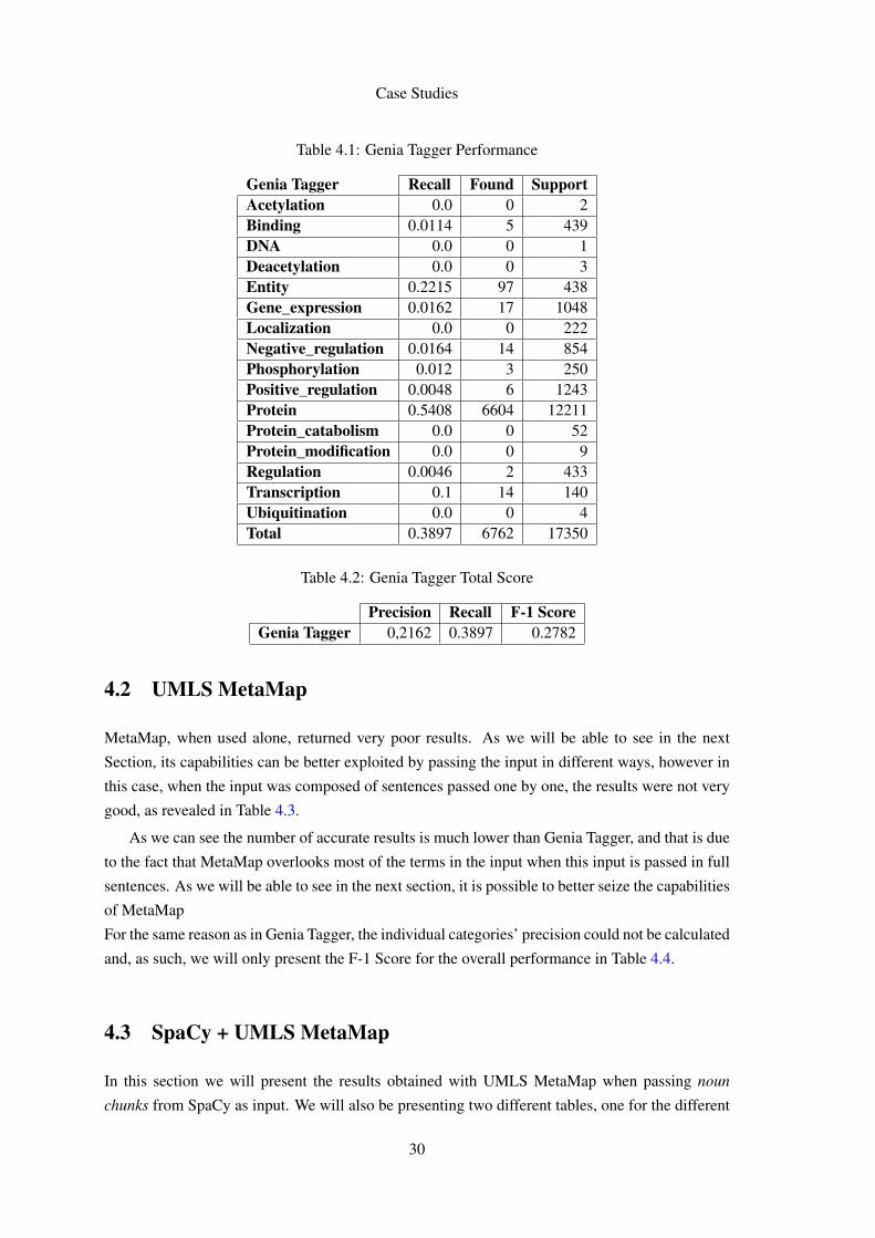
In Table 4.1, we can see the number denotations that Genia Tagger managed to find. We expected
it to perform a bit better, considering the scores from Table 2.2, however, we later recognized
that the way we use Genia Tagger could be improved, since we’re not taking advantage of the
chunktags it returns, but this will be later discussed in Section 5.2. Nevertheless, it is not clear
how much of an improvement we could get, or if those scores would be reached.
In Table 4.2 we can find the F-1 score for the overall performance of Genia Tagger. We did
not use this format in the previous Table 4.1, because it was not possible to calculate the precision
for the individual types of objects. This is because, when the results are returned, the tool does
not label those results with the same category as the denotations (obj field), at least not with the
same words. As such, we could not determine the false positives (results that are returned, but are
not correct solutions) for the individual categories, we could only do it for the overall performance
seeing that we know the total number of results.
29
Case Studies
Table 4.1: Genia Tagger Performance
Genia Tagger Recall Found SupportAcetylation 0.0 0 2Binding 0.0114 5 439DNA 0.0 0 1Deacetylation 0.0 0 3Entity 0.2215 97 438Gene_expression 0.0162 17 1048Localization 0.0 0 222Negative_regulation 0.0164 14 854Phosphorylation 0.012 3 250Positive_regulation 0.0048 6 1243Protein 0.5408 6604 12211Protein_catabolism 0.0 0 52Protein_modification 0.0 0 9Regulation 0.0046 2 433Transcription 0.1 14 140Ubiquitination 0.0 0 4Total 0.3897 6762 17350
Table 4.2: Genia Tagger Total Score
Precision Recall F-1 ScoreGenia Tagger 0,2162 0.3897 0.2782
4.2 UMLS MetaMap
MetaMap, when used alone, returned very poor results. As we will be able to see in the next
Section, its capabilities can be better exploited by passing the input in different ways, however in
this case, when the input was composed of sentences passed one by one, the results were not very
good, as revealed in Table 4.3.
As we can see the number of accurate results is much lower than Genia Tagger, and that is due
to the fact that MetaMap overlooks most of the terms in the input when this input is passed in full
sentences. As we will be able to see in the next section, it is possible to better seize the capabilities
of MetaMap
For the same reason as in Genia Tagger, the individual categories’ precision could not be calculated
and, as such, we will only present the F-1 Score for the overall performance in Table 4.4.
4.3 SpaCy + UMLS MetaMap
In this section we will present the results obtained with UMLS MetaMap when passing noun
chunks from SpaCy as input. We will also be presenting two different tables, one for the different
30
Case Studies
Table 4.3: UMLS MetaMap Performance
UMLS MetaMap Recall Found SupportAcetylation 0.0 0 2Binding 0.0228 14 439DNA 0.0 0 1Deacetylation 0.0 0 3Entity 0.0502 22 438Gene_expression 0.0897 94 1048Localization 0.0045 1 222Negative_regulation 0.0258 23 854Phosphorylation 0.1120 28 250Positive_regulation 0.0459 57 1243Protein 0.0991 1215 12211Protein_catabolism 0.0 0 52Protein_modification 0.0 0 9Regulation 0.0185 8 433Transcription 0.0214 3 140Ubiquitination 0.0 0 4Total 0.0844 1465 17350
Table 4.4: UMLS MetaMap Total Score
Precision Recall F-1 ScoreUMLS MetaMap 0,0195 0.0844 0.0317
types of categories, Table 4.5, and another one with the score of the overall performance, Table
4.6.
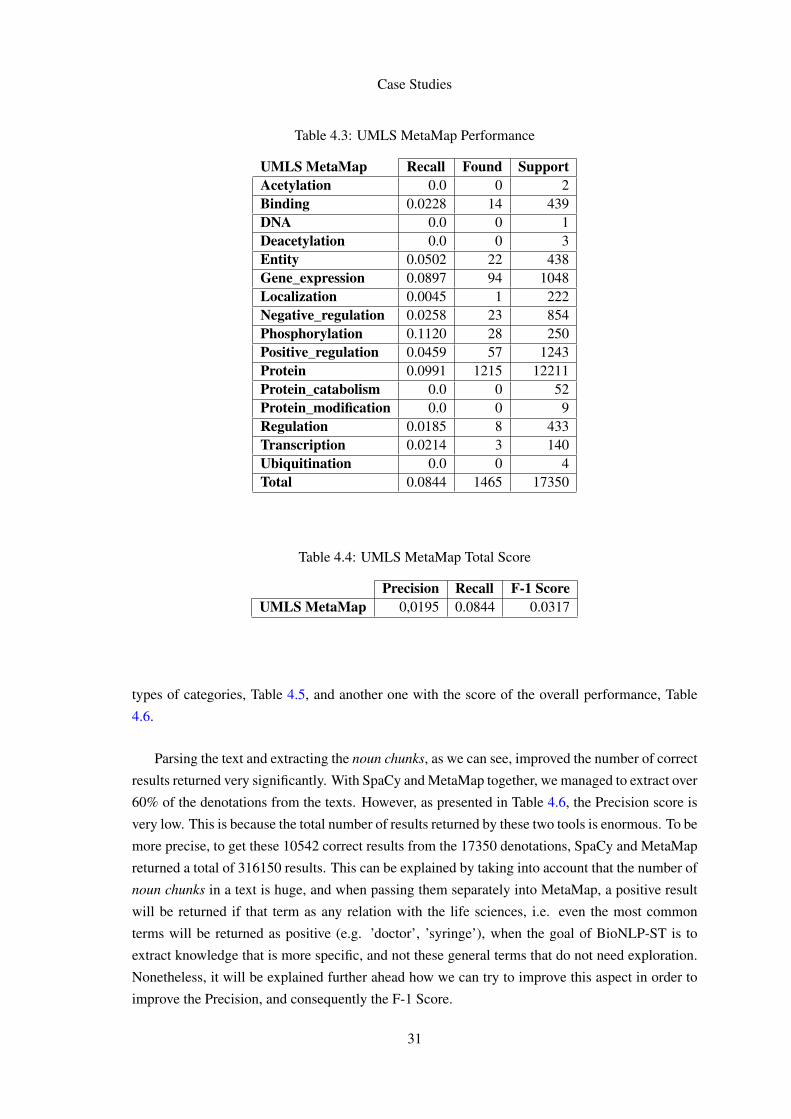
Parsing the text and extracting the noun chunks, as we can see, improved the number of correct
results returned very significantly. With SpaCy and MetaMap together, we managed to extract over
60% of the denotations from the texts. However, as presented in Table 4.6, the Precision score is
very low. This is because the total number of results returned by these two tools is enormous. To be
more precise, to get these 10542 correct results from the 17350 denotations, SpaCy and MetaMap
returned a total of 316150 results. This can be explained by taking into account that the number of
noun chunks in a text is huge, and when passing them separately into MetaMap, a positive result
will be returned if that term as any relation with the life sciences, i.e. even the most common
terms will be returned as positive (e.g. ’doctor’, ’syringe’), when the goal of BioNLP-ST is to
extract knowledge that is more specific, and not these general terms that do not need exploration.
Nonetheless, it will be explained further ahead how we can try to improve this aspect in order to
improve the Precision, and consequently the F-1 Score.
31

Case Studies
Table 4.5: SpaCy + UMLS MetaMap Performance
SpaCy + UMLS MetaMap Recall Found SupportAcetylation 1.0 2 2Binding 0.5718 251 439DNA 0.0 0 1Deacetylation 1.0 3 3Entity 0.4384 192 438Gene_expression 0.645 676 1048Localization 0.455 101 222Negative_regulation 0.4707 402 854Phosphorylation 0.676 169 250Positive_regulation 0.4867 605 1243Protein 0.636 7766 12211Protein_catabolism 0.7692 40 52Protein_modification 0.2222 2 9Regulation 0.5127 222 433Transcription 0.7786 109 140Ubiquitination 0.5 2 4Total 0.6076 10542 17350
Table 4.6: SpaCy + UMLS MetaMap Total Score
Precision Recall F-1 ScoreSpacy + UMLS MetaMap 0.1247 0.6076 0.2069
4.4 Final Results
Finally, we merge all the results from the separate tools presented above, in order to obtain the
final results from the whole process. Like before, we will display a table with the performance for
the different categories, Table 4.7, and another one for the overall score Table 4.8.
Taking into account all the scores displayed before for all the tools separately, the final total
results are in accordance to what was expected, i.e. a high score of Recall and a low score of
Precision, which means that even though a big majority of the denotations were found, raising the
Recall, there were lot of false positives being returned, which lowered Precision to a bigger extent,
which in the end pulled the final F-1 Score to a low value.
4.5 OHSUMED Corpus
Using the data mining software Weka, we ran some Classification algorithms on the texts from
the OHSUMED Corpus. We will present the tables with the respective results for the following
algorithms: J48 Decision Tree in Table 4.9, Random Forest in Table 4.11, Stochastic Gradient
Descent (SGD, SVM) in Table 4.13 and IBk (Nearest Neighbor) in Table 4.15.
We used 10-fold Cross Validation to divide the dataset into training sets and test sets. This means
32

Case Studies
Table 4.7: Final Process Performance
Complete Process Recall Found SupportAcetylation 1.0 2 2Binding 0.5809 255 439DNA 0.0 0 1Deacetylation 1.0 3 3Entity 0.5091 223 438Gene_expression 0.6584 690 1048Localization 0.455 101 222Negative_regulation 0.4883 417 854Phosphorylation 0.684 171 250Positive_regulation 0.5012 623 1243Protein 0.7492 9149 12211Protein_catabolism 0.7692 40 52Protein_modification 0.2222 2 9Regulation 0.5173 224 433Transcription 0.7857 110 140Ubiquitination 0.5 2 4Total 0.6923 12012 17350
Table 4.8: Final Process Total Score
Precision Recall F-1 ScoreFinal Process 0.0705 0.6923 0.1279
that the original data set is divided in 10 groups, and then the model will be run 10 times. In each
of those times one of the groups will be the test set while the other 9 will be the training set. This
way, all of the data will be both part of the training set and the test set. In the end the results will
be an average of the results from each run.
After adding the new found terms as attributes to the dataset, we ran all the algorithms again
with the new dataset, hoping for an improvement in the Classification scores. The results for
J48 Decision Tree can be seen in Table 4.10, Random Forest in Table 4.12, Stochastic Gradient
Descent (SGD, SVM) in Table 4.14 and IBk (Nearest Neighbor) in Table 4.16.
Table 4.9: J48 Classification Performance
J48 Precision Recall F-1 ScoreRELEVANT 0.934 0.916 0.925NON_RELEVANT 0.913 0.932 0.924Average 0.924 0.924 0.923
33

Case Studies
Table 4.10: J48 Classification Performance with new Dataset
J48 Precision Recall F-1 ScoreRELEVANT 0.918 0.948 0.933NON_RELEVANT 0.944 0.912 0.927Average 0.931 0.930 0.930
Table 4.11: Random Forest Classification Performance
Random Forest Precision Recall F-1 ScoreRELEVANT 0.849 0.916 0.881NON_RELEVANT 0.904 0.830 0.865Average 0.876 0.874 0.873
Table 4.12: Random Forest Classification Performance with New Dataset
Random Forest Precision Recall F-1 ScoreRELEVANT 0.800 0.883 0.840NON_RELEVANT 0.863 0.769 0.813Average 0.831 0.827 0.827
Table 4.13: SGD Classification Performance
SGD Precision Recall F-1 ScoreRELEVANT 0.811 0.838 0.824NON_RELEVANT 0.824 0.796 0.810Average 0.817 0.817 0.817
Table 4.14: SGD Classification Performance with new Dataset
SGD Precision Recall F-1 ScoreRELEVANT 0.825 0.825 0.825NON_RELEVANT 0.816 0.816 0.816Average 0.821 0.821 0.821
Table 4.15: IBk Classification Performance
IBk Precision Recall F-1 ScoreRELEVANT 0.513 0.929 0.661NON_RELEVANT 0.500 0.075 0.130Average 0.506 0.512 0.402
Table 4.16: IBk Classification Performance with new Dataset
IBk Precision Recall F-1 ScoreRELEVANT 0.513 0.903 0.654NON_RELEVANT 0.500 0.102 0.169Average 0.507 0.512 0.417
34

Case Studies
4.6 Chapter Summary
As mentioned before, the process developed did return relevant results, as revealed by the Recall
Score, however, at the same time it also returned a lot of irrelevant ones, which affected strongly
the final F-1 Score. Given the time constraints the process could not be perfected, even though we
recognize that there are aspects that could be improved. For instance, the usage of Genia Tagger
could be improved by taking better advantage of its syntactical analysis capabilities in hope of
improving the number and accuracy of the results, i.e. using the chunktags it returns in order to
compose expressions with more than one word. Moreover, there could be an attempt of reducing
the number of irrelevant results from both the UMLS MetaMap method, by mapping the results
with other ontologies, thesaurus or dictionaries, in hopes of eliminating some of returned results.
Nevertheless, these results show promise seeing that a big part of the denotations were in fact
found.
As for the OHSUMED corpus, the results satisfied our expectations, seeing that, out of the four
algorithms chosen, the results improved slightly for three of them, having worsened for only for
the Random Forest algorithm.
35

Case Studies
36

Chapter 5
Conclusions
In this last chapter we will be discussing the accomplishments of this work, exploring on what
was done right, and what could have been improved, while trying to explain the meaning of these
accomplishments. Then we will expose some future work options, or methods and processes that
could be adopted in the following of this dissertation, that would improve and upgrade the current
process.
5.1 Accomplishments
As presented in Chapter 4, with the process we managed to extract over 69% of the denotations
from the BioNLP datasets. Even if this outcome, came at the cost of a really low Precision score,
we think it shows some promise, seeing that the most of the correct results are already being
returned, it is now a matter of perfecting the process in an attempt of reducing the number of
irrelevant results, thus improving the Precision.
Also in the previous chapter, we can see that the method that most contributed for the high Recall
score achieved was the conjugation of SpaCy with UMLS MetaMap, however, this method also
greatly lowered the Precision, along with MetaMap, due to the huge number of possible results it
returned. In comparison to the UMLS MetaMap run on its own, adding SpaCy did make a huge
impact on the results. As for Genia Tagger, the results were a bit disappointing, but we will be
addressing this situation in the next section.
Due to time constraints, this was what we could achieve, and thus we could not get into trying
to classify the results obtained, which would be the next step. Also, another goal of the BioNLP
Shared Task, was to extract the relations between entities and the modifications, which we also
did not manage to address. It took more time than anticipated to learn about Text Mining and all
the processes it involves, to really understand how everything works and how to proceed, specially
when I had no experience in this field. Time really was a set back, however, if we had more, we
think we would be able to really make some progress and improvements, as we have an idea of
37
Conclusions
how we would proceed, and as I am more informed and familiarized with this area, we have a
more clear thought on what would be needed to perform next.
The quality of the tool can also be proven through the analysis of the OHSUMED corpus, seeing
that three out of four Classification algorithms performed better when using a dataset with our
added attributes.
5.2 Future Work
Genia Tagger did not perform quite like we were expecting, having achieved a score that was
lower than what we hoped for. One of the reasons behind this, is the format of the output (Section
3.3). It will return the results word-by-word, and because of this, we are only handling one word
results. One way we think would improve its scores, is by taking advantage of the chunktags, in
an attempt of joining more than one word to obtain more results. These chunktags are presented
in the IOB2, which means that each word will have a tag associated, indicating where said word
is located in relation to the chunk it belongs to (e.g. in the expression "lung cancer", "lung" would
have a B tag, and "cancer" would have an I tag). With this, whenever we found a word with an "I"
tag, we could trace back the words until we find a "B" tag, allowing us to then obtain an expression
with more than one word, thus developing new results that were being overlooked before.
Another improvement to be implemented is a more extensive use of ontologies, thesaurus and dic-
tionaries in order to reduce the number of irrelevant results returned, mainly by the methods using
UMLS MetaMap. By searching the terms returned, we could eliminate the ones that found no
match, reducing the number of false positives and consequently improving the process’ precision.
We also had in mind using more tools in hopes of getting better and more results, however this
proved impossible due to the time constraints. There were a couple of tools that we tried embed-
ding in the process, however we did not manage to do it, seeing that we were already too late in
the game. We are referring to BANNER and ABNER, which present very good scores in NER for
Biomedical literature [LG08] [Set05]. Besides being too late in the game, we found these tools
to be harder to implement in the process for a number of reasons. For instance, both of the tools
were developed in Java which makes it harder to use in a python program. Also, none of the tools
could be run from the terminal, in ABNER’s case, it even had a Graphic interface, which made it
more challenging to call it and obtain the results, since it focused more on providing more graphic
results. Finally, there is not much support online, so we found it hard to discover a way of calling
these tools from a python program, seeing that we could not find guides or tutorials to work with
these tools, at least not updated ones. Besides these two tools, we also considered exploring and
experimenting with the Turku Event Extraction System.
After having extracted the maximum number of denotations with the best possible score, the next
step would be to classify them, using Data Mining Classification Algorithms. Provided by all the
extracted terms, the goal would the to classify them into one of the categories from the denota-
tions (Section 3.1, and 4 in the results tables). The performance of this Classification would later
38

Conclusions
be evaluated using the F-1 Score as well. This process would involve trying out different algo-
rithms in hopes of finding the one that would outperform the others and achieve the highest score.
After this whole process, and even though we were still a little bit far from this stage, the next
step would be to try to perform the Relation Extraction. We did not really get into it, however
we had already though about it. Some research was made about this part, and we discovered a
tool for this purpose, SemRep, which stands for Semantic Representation or Semantic Knowledge
Representation. It can be found in the National Institutes of Health website, and as they describe
it "SemRep is a UMLS-based program that extracts three-part propositions, called semantic pred-
ications, from sentences in biomedical text. Predications consist of a subject argument, an object
argument, and the relation that binds them"1 [RF03]. Using an example they provide, given the
sentence "We used hemofiltration to treat a patient with digoxin overdose that was complicated by
refractory hyperkalemia." SemRep extract the following predications 5.1.
1 Hemofiltration-TREATS-Patients
2 Digoxin overdose-PROCESS_OF-Patients
3 hyperkalemia-COMPLICATES-Digoxin overdose
4 Hemofiltration-TREATS(INFER)-Digoxin overdose
Listing 5.1: SemRep output
Since we have not tried to work with it, we cannot know for sure, but we expect it to be easy
to use since it is UMLS based, and it is from the National Library of Medicine, just like UMLS
MetaMap, so we do not expect it to be harder than it, moreover, it is available for Linux, which is
a good indication that it can run from the terminal, similarly to MetaMap.
1https://semrep.nlm.nih.gov/
39

Conclusions
40
References
[Aro96] Alan R Aronson. Metamap technical notes. Technical report, Technical report,United States National Library of Medicine, Bethesda, MD, 1996.
[Aro01] Alan R Aronson. Metamap evaluation. Unpublished manuscript, 2001.
[Bjö14] Jari Björne. Biomedical Event Extraction with Machine Learning. PhD thesis, Uni-versity of Turku, 2014.
[Blu04] Phil Blunsom. Hidden markov models. Lecture notes, August, 15(18-19):48, 2004.
[Bor12] Christine L. Borgman. The conundrum of sharing research data. Journal of theAmerican Society for Information Science and Technology, 63(6):1059–1078, April2012.
[Bre01] Leo Breiman. Random forests. Machine learning, 45(1):5–32, 2001.
[CH67] Thomas Cover and Peter Hart. Nearest neighbor pattern classification. IEEE trans-actions on information theory, 13(1):21–27, 1967.
[CL96] Jim Cowie and Wendy Lehnert. Information extraction. Communications of theACM, 39(1):80–91, 1996.
[CR10] Yee Seng Chan and Dan Roth. Exploiting background knowledge for relation ex-traction. In Proceedings of the 23rd International Conference on ComputationalLinguistics, pages 152–160. Association for Computational Linguistics, 2010.
[DD16] Miss Deepa S Deulkar and RR Deshmukh. Data mining classification. ImperialJournal of Interdisciplinary Research, 2(4), 2016.
[GCP14] Sonali Vijay Gaikwad, Archana Chaugule, and Pramod Patil. Text mining meth-ods and techniques. International Journal of Computer Applications, 85(17):42–45,January 2014.
[gen] Genia tagger. available at http://www.nactem.ac.uk/GENIA/tagger/. Ac-cessed: 2018-06-20.
[GIB+18] Carlos Gonçalves, Eva Lorenzo Iglesias, Lourdes Borrajo, Rui Camacho, A SearaVieira, and Célia Talma Gonçalves. Learnsec: A framework for full text analysis. InInternational Conference on Hybrid Artificial Intelligence Systems, pages 502–513.Springer, 2018.
[HBLH94] William Hersh, Chris Buckley, TJ Leone, and David Hickam. Ohsumed: an inter-active retrieval evaluation and new large test collection for research. In SIGIR’94,pages 192–201. Springer, 1994.
41

REFERENCES
[HNP05] Andreas Hotho, Andreas Nürnberger, and Gerhard Paass. A brief survey of textmining. 20:19–62, 01 2005.
[Hua] Steeve Huang. Word2vec and fasttext word embedding with gensim. To-wards Data Science, available at https://towardsdatascience.com/word-embedding-with-word2vec-and-fasttext-a209c1d3e12c. Ac-cessed: 2018-06-15.
[Jha12] Alok Jha. Text mining: what do publishers have against this hi-tech research tool?Technical report, The Guardian, May 2012.
[KKHRS15] Jin-Dong Kim, Jung-jae Kim, Xu Han, and Dietrich Rebholz-Schuhmann. Extend-ing the evaluation of genia event task toward knowledge base construction and com-parison to gene regulation ontology task. BMC bioinformatics, 16(10):S3, 2015.
[LA99] Bjornar Larsen and Chinatsu Aone. Fast and effective text mining using linear-time document clustering. In Proceedings of the fifth ACM SIGKDD internationalconference on Knowledge discovery and data mining, pages 16–22. ACM, 1999.
[LdC07] Ana Carolina Lorena and André CPLF de Carvalho. Uma introdução às supportvector machines. Revista de Informática Teórica e Aplicada, 14(2):43–67, 2007.
[Lei17] Vânia Leite. Biological Processes Identification in Texts. PhD thesis, Universidadedo Porto, 2017.
[LG08] Robert Leaman and Graciela Gonzalez. Banner: an executable survey of advancesin biomedical named entity recognition. In Biocomputing 2008, pages 652–663.World Scientific, 2008.
[nlm] U.s. national library of medicine. By U.s. Department of Health and Human Ser-vices, available at https://www.nlm.nih.gov/. Accessed: 2018-06-20.
[RE09] Raul Rodriguez-Esteban. Biomedical text mining and its applications. PLoS com-putational biology, 5(12):e1000597, 2009.
[RF03] Thomas C Rindflesch and Marcelo Fiszman. The interaction of domain knowledgeand linguistic structure in natural language processing: interpreting hypernymicpropositions in biomedical text. Journal of biomedical informatics, 36(6):462–477,2003.
[Set05] Burr Settles. Abner: an open source tool for automatically tagging genes, proteinsand other entity names in text. Bioinformatics, 21(14):3191–3192, 2005.
[Sil14] Matheus Coppetti Silveira. Named entity recognition. 2014.
[spa] Spacy - industrial-strength natural language processing. By Explosion AI, availableat https://spacy.io/. Accessed: 2018-06-20.
[uml] Unified medical language system (umls). By U.s. Department of Health and HumanServices, available at https://www.nlm.nih.gov/research/umls/. Ac-cessed: 2018-06-20.
[VSM] Vector space model. Technical University of Denmark, available at http://cogsys.imm.dtu.dk/thor/projects/multimedia/textmining/node5.html. Accessed: 2018-06-15.
42

REFERENCES
[Wal06] Hanna M Wallach. Topic modeling: beyond bag-of-words. In Proceedings of the23rd international conference on Machine learning, pages 977–984. ACM, 2006.
[ZDFYC07] Pierre Zweigenbaum, Dina Demner-Fushman, Hong Yu, and Kevin B Cohen. Fron-tiers of biomedical text mining: current progress. Briefings in bioinformatics,8(5):358–375, 2007.
43

REFERENCES
44

Appendix A
POS Tags
A list of all the Part of Speech Tags.
1 CC Coordinating conjunction
2 CD Cardinal number
3 DT Determiner
4 EX Existential there
5 FW Foreign word
6 IN Preposition or subordinating conjunction
7 JJ Adjective
8 JJR Adjective, comparative
9 JJS Adjective, superlative
10 LS List item marker
11 MD Modal
12 NN Noun, singular or mass
13 NNS Noun, plural
14 NNP Proper noun, singular
15 NNPS Proper noun, plural
16 PDT Predeterminer
17 POS Possessive ending
18 PRP Personal pronoun
19 PRP$ Possessive pronoun
20 RB Adverb
21 RBR Adverb, comparative
22 RBS Adverb, superlative
23 RP Particle
24 SYM Symbol
25 TO to
26 UH Interjection
27 VB Verb, base form
28 VBD Verb, past tense
29 VBG Verb, gerund or present participle
30 VBN Verb, past participle
31 VBP Verb, non-3rd person singular present
32 VBZ Verb, 3rd person singular present
45

POS Tags
33 WDT Wh-determiner
34 WP Wh-pronoun
35 WP$ Possessive wh-pronoun
36 WRB Wh-adverb
46

Appendix B
UMLS Semantic Types and Groups
A list of the semantic types and groups recognized by UMLS MetaMap (the first line is the repre-
sentation format).
1 Semantic Group Abbrev|Semantic Group Name|Type Unique Identifier (TUI)|Full
Semantic Type Name
2
3 ACTI|Activities & Behaviors|T052|Activity
4 ACTI|Activities & Behaviors|T053|Behavior
5 ACTI|Activities & Behaviors|T056|Daily or Recreational Activity
6 ACTI|Activities & Behaviors|T051|Event
7 ACTI|Activities & Behaviors|T064|Governmental or Regulatory Activity
8 ACTI|Activities & Behaviors|T055|Individual Behavior
9 ACTI|Activities & Behaviors|T066|Machine Activity
10 ACTI|Activities & Behaviors|T057|Occupational Activity
11 ACTI|Activities & Behaviors|T054|Social Behavior
12 ANAT|Anatomy|T017|Anatomical Structure
13 ANAT|Anatomy|T029|Body Location or Region
14 ANAT|Anatomy|T023|Body Part, Organ, or Organ Component
15 ANAT|Anatomy|T030|Body Space or Junction
16 ANAT|Anatomy|T031|Body Substance
17 ANAT|Anatomy|T022|Body System
18 ANAT|Anatomy|T025|Cell
19 ANAT|Anatomy|T026|Cell Component
20 ANAT|Anatomy|T018|Embryonic Structure
21 ANAT|Anatomy|T021|Fully Formed Anatomical Structure
22 ANAT|Anatomy|T024|Tissue
23 CHEM|Chemicals & Drugs|T116|Amino Acid, Peptide, or Protein
24 CHEM|Chemicals & Drugs|T195|Antibiotic
25 CHEM|Chemicals & Drugs|T123|Biologically Active Substance
26 CHEM|Chemicals & Drugs|T122|Biomedical or Dental Material
27 CHEM|Chemicals & Drugs|T118|Carbohydrate
28 CHEM|Chemicals & Drugs|T103|Chemical
29 CHEM|Chemicals & Drugs|T120|Chemical Viewed Functionally
30 CHEM|Chemicals & Drugs|T104|Chemical Viewed Structurally
47
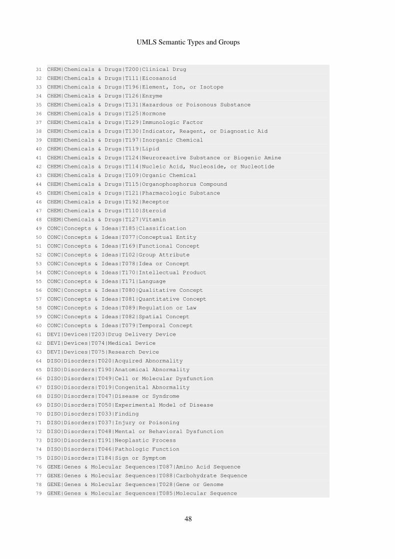
UMLS Semantic Types and Groups
31 CHEM|Chemicals & Drugs|T200|Clinical Drug
32 CHEM|Chemicals & Drugs|T111|Eicosanoid
33 CHEM|Chemicals & Drugs|T196|Element, Ion, or Isotope
34 CHEM|Chemicals & Drugs|T126|Enzyme
35 CHEM|Chemicals & Drugs|T131|Hazardous or Poisonous Substance
36 CHEM|Chemicals & Drugs|T125|Hormone
37 CHEM|Chemicals & Drugs|T129|Immunologic Factor
38 CHEM|Chemicals & Drugs|T130|Indicator, Reagent, or Diagnostic Aid
39 CHEM|Chemicals & Drugs|T197|Inorganic Chemical
40 CHEM|Chemicals & Drugs|T119|Lipid
41 CHEM|Chemicals & Drugs|T124|Neuroreactive Substance or Biogenic Amine
42 CHEM|Chemicals & Drugs|T114|Nucleic Acid, Nucleoside, or Nucleotide
43 CHEM|Chemicals & Drugs|T109|Organic Chemical
44 CHEM|Chemicals & Drugs|T115|Organophosphorus Compound
45 CHEM|Chemicals & Drugs|T121|Pharmacologic Substance
46 CHEM|Chemicals & Drugs|T192|Receptor
47 CHEM|Chemicals & Drugs|T110|Steroid
48 CHEM|Chemicals & Drugs|T127|Vitamin
49 CONC|Concepts & Ideas|T185|Classification
50 CONC|Concepts & Ideas|T077|Conceptual Entity
51 CONC|Concepts & Ideas|T169|Functional Concept
52 CONC|Concepts & Ideas|T102|Group Attribute
53 CONC|Concepts & Ideas|T078|Idea or Concept
54 CONC|Concepts & Ideas|T170|Intellectual Product
55 CONC|Concepts & Ideas|T171|Language
56 CONC|Concepts & Ideas|T080|Qualitative Concept
57 CONC|Concepts & Ideas|T081|Quantitative Concept
58 CONC|Concepts & Ideas|T089|Regulation or Law
59 CONC|Concepts & Ideas|T082|Spatial Concept
60 CONC|Concepts & Ideas|T079|Temporal Concept
61 DEVI|Devices|T203|Drug Delivery Device
62 DEVI|Devices|T074|Medical Device
63 DEVI|Devices|T075|Research Device
64 DISO|Disorders|T020|Acquired Abnormality
65 DISO|Disorders|T190|Anatomical Abnormality
66 DISO|Disorders|T049|Cell or Molecular Dysfunction
67 DISO|Disorders|T019|Congenital Abnormality
68 DISO|Disorders|T047|Disease or Syndrome
69 DISO|Disorders|T050|Experimental Model of Disease
70 DISO|Disorders|T033|Finding
71 DISO|Disorders|T037|Injury or Poisoning
72 DISO|Disorders|T048|Mental or Behavioral Dysfunction
73 DISO|Disorders|T191|Neoplastic Process
74 DISO|Disorders|T046|Pathologic Function
75 DISO|Disorders|T184|Sign or Symptom
76 GENE|Genes & Molecular Sequences|T087|Amino Acid Sequence
77 GENE|Genes & Molecular Sequences|T088|Carbohydrate Sequence
78 GENE|Genes & Molecular Sequences|T028|Gene or Genome
79 GENE|Genes & Molecular Sequences|T085|Molecular Sequence
48
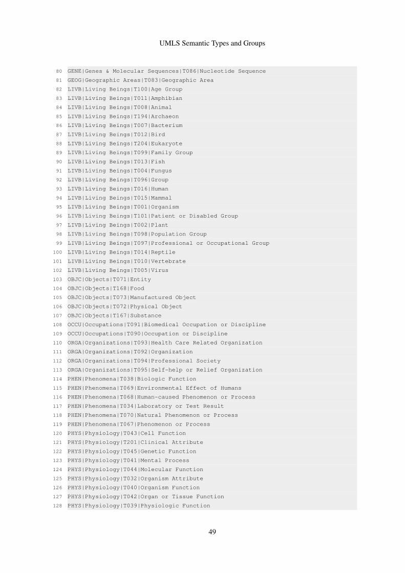
UMLS Semantic Types and Groups
80 GENE|Genes & Molecular Sequences|T086|Nucleotide Sequence
81 GEOG|Geographic Areas|T083|Geographic Area
82 LIVB|Living Beings|T100|Age Group
83 LIVB|Living Beings|T011|Amphibian
84 LIVB|Living Beings|T008|Animal
85 LIVB|Living Beings|T194|Archaeon
86 LIVB|Living Beings|T007|Bacterium
87 LIVB|Living Beings|T012|Bird
88 LIVB|Living Beings|T204|Eukaryote
89 LIVB|Living Beings|T099|Family Group
90 LIVB|Living Beings|T013|Fish
91 LIVB|Living Beings|T004|Fungus
92 LIVB|Living Beings|T096|Group
93 LIVB|Living Beings|T016|Human
94 LIVB|Living Beings|T015|Mammal
95 LIVB|Living Beings|T001|Organism
96 LIVB|Living Beings|T101|Patient or Disabled Group
97 LIVB|Living Beings|T002|Plant
98 LIVB|Living Beings|T098|Population Group
99 LIVB|Living Beings|T097|Professional or Occupational Group
100 LIVB|Living Beings|T014|Reptile
101 LIVB|Living Beings|T010|Vertebrate
102 LIVB|Living Beings|T005|Virus
103 OBJC|Objects|T071|Entity
104 OBJC|Objects|T168|Food
105 OBJC|Objects|T073|Manufactured Object
106 OBJC|Objects|T072|Physical Object
107 OBJC|Objects|T167|Substance
108 OCCU|Occupations|T091|Biomedical Occupation or Discipline
109 OCCU|Occupations|T090|Occupation or Discipline
110 ORGA|Organizations|T093|Health Care Related Organization
111 ORGA|Organizations|T092|Organization
112 ORGA|Organizations|T094|Professional Society
113 ORGA|Organizations|T095|Self-help or Relief Organization
114 PHEN|Phenomena|T038|Biologic Function
115 PHEN|Phenomena|T069|Environmental Effect of Humans
116 PHEN|Phenomena|T068|Human-caused Phenomenon or Process
117 PHEN|Phenomena|T034|Laboratory or Test Result
118 PHEN|Phenomena|T070|Natural Phenomenon or Process
119 PHEN|Phenomena|T067|Phenomenon or Process
120 PHYS|Physiology|T043|Cell Function
121 PHYS|Physiology|T201|Clinical Attribute
122 PHYS|Physiology|T045|Genetic Function
123 PHYS|Physiology|T041|Mental Process
124 PHYS|Physiology|T044|Molecular Function
125 PHYS|Physiology|T032|Organism Attribute
126 PHYS|Physiology|T040|Organism Function
127 PHYS|Physiology|T042|Organ or Tissue Function
128 PHYS|Physiology|T039|Physiologic Function
49

UMLS Semantic Types and Groups
129 PROC|Procedures|T060|Diagnostic Procedure
130 PROC|Procedures|T065|Educational Activity
131 PROC|Procedures|T058|Health Care Activity
132 PROC|Procedures|T059|Laboratory Procedure
133 PROC|Procedures|T063|Molecular Biology Research Technique
134 PROC|Procedures|T062|Research Activity
135 PROC|Procedures|T061|Therapeutic or Preventive Procedure
50