texpoint fonts used in emf. read the texpoint manual before you delete this box.: a a

Sumit Gulwani(Microsoft Research, Redmond)

The Reachability-Bound Problem

Florian Zuleger(TU Darmstadt)

Sudeep Juvekar(UC-Berkeley)

Joint work with

Let ¼ be some control location inside a procedure.

• Safety: Is ¼ never visited?– Violation is a finite trace

• Liveness: Is ¼ visited at most finite number of times?– Violation is an infinite trace

• Reachability-Bound: Symbolic bound on maximum visits to ¼.– Quantitative question as opposed to Boolean.– Checking validity of a given bound is a safety property.– Checking precision is not even a trace property.– The problem is challenging!

2

The Reachability-Bound Problem

• Programs consume a variety of resources.– CPU time, Memory, Network Bandwidth, Power

• It is important to bound use of such resources.– Economic incentives– Better user experience– Hard constraints on availability of resources

• Real-time/embedded systems, Low power/bandwidth devices

• This requires computing bounds on # of visits to control-locations that consume these resources.– Memory Allocated = §¼ [Visits(¼) £ BytesAllocated(¼)]

– Asymptotic Time Complexity = §H [Visits(H)], where H ranges over loop headers. 3

Motivation 1: Resource Bound Analysis

• Program execution affects certain quantitative properties of data.– Secrecy: information leakage.– Robustness: error/uncertainty propagation.

• Bounding such properties requires computing bound on # of visits to control-locations that affect such properties of the data.

4

Motivation 2: Quantitative Analysis of Data

• Time Complexity = Visits(¼1) + Visits(¼2)– Visits(¼1) · n and Visits(¼2) · n2

• Memory Allocated = Visits(¼3) £ SizeOf(C)

– Visits(¼3) · n2

5

Example (.Net Library)

Inputs: int n, bool[] A i := 0; ¼1: while (i < n) { j := i+1; ¼2: while (j < n) { if (A[j]) { ¼3: B[n] := new C(); } j++; } i++; }

• Time Complexity = Visits(¼1) + Visits(¼2)– Visits(¼1) · n and Visits(¼2) · n2

• Memory Allocated = Visits(¼3) £ SizeOf(C)

– Visits(¼3) · n

– Nested loop does not necessarily imply quadratic complexity. 6


Inputs: int n, bool[] A i := 0; ¼1: while (i < n) { j := i+1; ¼2: while (j < n) { if (A[j]) { ¼3: B[n] := new C(); j--; n--; } j++; } i++; }

Examine the loop induced by the control-flow graph starting at , and the next visit to it.

• Loop has one path.– Compute ranking function using constraint-based or

proof rules based technique.• Loop has multiple paths.

– Compose ranking functions for paths using proof rules.– One proof rule each for Max, Sum, and Product

composition.• Loop has inner loops.

– Summarize inner loops by precise disjunctive invariants using forward iterative technique (abstract interpretation).

• Loop has other loops before it.– Perform backward symbolic execution (using proof

rules to trace across loops) to express bound in terms of inputs.

7

Algorithm: A variety of fixed-point techniques


Loop has one path.– Compute ranking function using constraint-based or

proof rules based technique.• Loop has multiple paths.






8


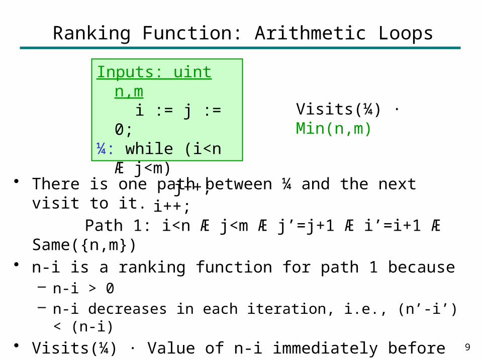
• There is one path between ¼ and the next visit to it. Path 1: i<n Æ j<m Æ j’=j+1 Æ i’=i+1 Æ

Same({n,m}) • n-i is a ranking function for path 1 because

– n-i > 0– n-i decreases in each iteration, i.e., (n’-i’) < (n-i)

• Visits(¼) · Value of n-i immediately before the loop = n

• Similarly, m-j is also a ranking function and Visits(¼) · m

9

Ranking Function: Arithmetic Loops

Inputs: uint n,m i := j := 0;¼: while (i<n Æ

j<m) j++;

i++;

Visits(¼) · Min(n,m)

• Guess a ranking function e– For each (syntactically appearing) inequality e1 ¸

e2 in P, guess e1-e2 to be a candidate.

• Check whether e is a ranking function by validating the following constraints using an SMT solver.

P ) e¸0 P ) (e[X’/X] · e-1)

• The proof rule based technique extends readily to cases other than integer arithmetic.– E.g., loops that iterate over bit-vectors or data-

structures 10

Computing Ranking Functions: Proof Rule Technique

• The proof-rule based technique is not complete. Consider the following example.– P: x¸0 Æ y¸0 Æ x’=y Æ y’=x-1– Neither x nor y is a ranking function, but x+y is.

• There is a “complete” method to find linear ranking functions [Podelski, Rybalchenko, VMCAI ‘04] – Let ranking function be of form a1x + a2y + a3

– We want to find a1, a2, a3 such that for all x,y

• P ) (a1x+a2y+a3) ¸ 0 and

• P ) (a1x’+a2y’+a3) · (a1x+a2y+a3) -1– Farkas Lemma can be used to reduces the above

system of quantified equations to that of linear inequalities.

11

Computing Ranking Functions: Constraint-based Technique

Ranking Function: Bitvector Loops (SQL)

12

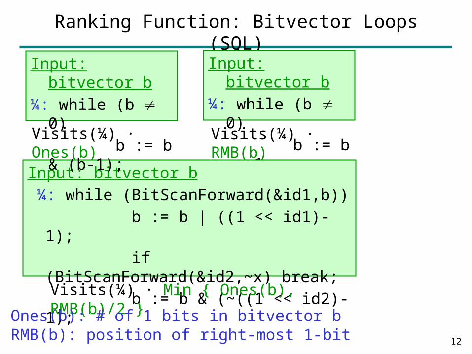
Input: bitvector b¼: while (b 0) b := b <<

1;Visits(¼) · RMB(b)

Input: bitvector b ¼: while (BitScanForward(&id1,b)) b := b | ((1 << id1)-1); if (BitScanForward(&id2,~x)

break; b := b & (~((1 << id2)-1);

Visits(¼) · Min { Ones(b), RMB(b)/2 }

Input: bitvector b¼: while (b 0) b := b & (b-

1);Visits(¼) · Ones(b)

Ones(b): # of 1 bits in bitvector bRMB(b): position of right-most 1-bit

Ranking Function: Data-structure Loops

13

Input: List L¼: while (L Null) L := L.Next;

Visits(¼) · Length(L, Next)

Input: ICollection C¼: foreach(Element e in

C) …Requires analysis of C.MoveNext() method.In case of virtual method, we define Visits(¼) to be C.count



proof rule based technique. Loop has multiple paths.






14


Composition of Ranking Functions

15

Inputs: uint n,m

i := j := 0;¼: while (i<n) if (j<m)

j++; else i++;

Visits(¼) · n + m

Inputs: uint n,m i := j := 0;¼: while (i<n) if (j<m) j++;

else {i++; j:=0;}

Visits(¼) · n £ (1+m)

Inputs: uint n,m i := j := 0;¼: while (j<m Ç

i<n) j++; i++;

Visits(¼) · Max(n,m)

Path 1: j<m Æ j’=j+1 Æ i’=i+1Path 2: i<n Æ j’=j+1 Æ i’=i+1

Path 1: i<n Æ j<m Æ j’=j+1 Path 2: i<n Æ j¸m Æ i’=i+1

Path 1: i<n Æ j<m Æ j’=j+1 Path 2: i<n Æ j¸m Æ i’=i+1 Æ j’=0

Let r1, r2 be ranking functions for p1, p2 respectively. Non-Interference NI(p1,p2,r2):• Non-enabling condition: p1 ± p2 = false• Rank preserving condition: p1 ) r2[x’/x] · r2

Proof Rule: If NI(p1,p2,r2) and NI(p2,p1,r1), then: Bound(p1 Ç p2) =

Example: p1: (i<n Æ i’=i+1 Æ Same({j,n,m}) )p2: (j<m Æ j’=j+1 Æ Same({i,n,m}) )r1: n-i, r2: m-jBound(p1 Ç p2) = Max(0, n-i) + Max(0, m-j) = n + m

16

Proof Rule for Additive Composition

Max(0, r1) + Max(0,r2)

Let r1, r2 be ranking functions for p1, p2 respectively.

Proof Rule: If NI(p2,p1,r1), then: Bound(p1 Ç p2) =

where u2(X) is an upper bound on r2[X’/X] as implied by p1.

Example: p1: (i<n Æ i’=i+1 Æ j’=0 Æ Same({n,m}))p2: (j<m Æ j’=j+1 Æ Same({i,n,m}))r1: n-i, r2: m-jBound(p1 Ç p2) = Max(0,n-i) * [1 + Max(0,m-j)] = n * (1+m) 17

Proof Rule for Multiplicative Composition

Max(0,r1) + Max(0,r2) + Max(0,u2)*Max(0,r1)

Let r1, r2 be ranking functions for p1, p2 respectively. Cooperative Interference CI(p1,r1,p2,r2):• Non-enabling condition: p1 ± p2 = false• Rank decrease condition: p1 ) r2[x’/x] · Max(r1,r2)-

1

Proof Rule: If CI(p1, r1, p2, r2) and CI(p2,r2,p1,r1), then:

Bound(p1 Ç p2) =

Example: p1: (i<n Æ i’=i+1 Æ j’=j+1 Æ Same({n,m}) )p2: (j<m Æ i’=i+1 Æ j’=j+1 Æ Same({n,m}) )r1: n-i, r2: m-jBound(p1 Ç p2) = Max(0, n-i, m-j) = Max(n,m)

18

Proof Rule for Max Composition

Max(0, r1, r2)



proof rule based technique.• Loop has multiple paths.


composition. Loop has inner loops.




19


• A loop with body T can be replaced by TransitiveClosure(T).

• We say that a relation R is TransitiveClosure(T) if Id ) R and R ± T ) R where Id is the relation X’=X

• Precise transitive closures can be computed using iterative fixed-point techniques such as abstract interpretation or model checking.

• Example of TransitiveClosure(s1 Ç s2)

20

Transitive Closure

s1: i’=i+1 Æ j’=0

s2: i’=i Æ j’=j+1

(i’¸i+1 Æ j’¸0) Ç (i’=i Æ j’¸j)

Visits(¼3) · n

21


Inputs: int n, bool[] A i := 0; ¼1: while (i < n) { j := i+1; ¼2: while (j < n) { if (A[j]) { ¼3: B[n] := new C(); j--; n--; } j++; } i++; }

22

Split Control Location

B[n] := new C;

yesπ3j--;n--;

no A[j]

i := 0;

j := i+1;

i := i+1;

j := j+1;

yes

yes

no

no

end

i < n

j < n

begin

B[n] := new C;

j--;n--;

yesno

π3a

A[j] π3b

i := 0;

j := i+1;

i := i+1;

j := j+1;

yes

yes

no

no

begin

end

i < n

j < n

23

Split Control Location

B[n] := new C;

j--;n--;

yesno

π3a

A[j] π3b

i := 0;

j := i+1;

i := i+1;

j := j+1;

yes

yes

no

no

begin

end

i < n

j < n

j := i+1;

i := i+1;

B[n] := new C;

j := j+1;

j--;n--;

π3a

π3b

yes

yes

yes

no

no

i < nj < n

A[j]

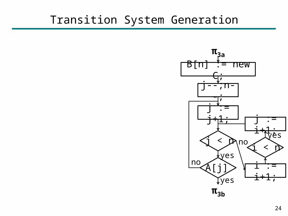
j < n

24

Transition System Generation

j := i+1;

i := i+1;

B[n] := new C;

j := j+1;

j--;n--;

π3a

π3b

yes

yes

yes

no

no

i < n

A[j]

j < n

• Transition-system T1 of inner loop (j¸n Æ i<n-1 Æ i’=i+1 Æ j’=i+2)• T1’ = Transitive Closure(T1) = (i’=iÆj’=j) Ç (j¸n Æ i<n-1 Æ i’>i Æ

j’¸i+2)

25


j := i+1;

i := i+1;

B[n] := new C;

j := j+1;

j--;n--;

π3a

π3b

yes

yes

yes

no

no

i < n

A[j]

• Transition-system T1 of inner loop: (j¸n Æ i<n-1 Æ i’=i+1 Æ j’=i+2)• T1’ = Transitive Closure(T1) = (i’=iÆj’=j) Ç (j¸n Æ i<n-1 Æ i’>i Æ

j’¸i+2)

26


B[n] := new C;

j := j+1;

j--;n--;

π3a

π3b

yes

noA[j]

T1‘


j’¸i+2)• Transition-system T2 of outer loop (j<n-1 Æj’=j+1 Æi’=i) Ç (i<n-1 Æi’>i

Æj’¸i+2)• T2’ = Transitive Closure(T2) = (j’¸j Æ i’=i) Ç (i<n-1 Æ i’>i Æ

j’¸i+2)

27


B[n] := new C;

j := j+1;

j--;n--;

π3a

π3b

yes

noA[j]

T1‘


j’¸i+2)• Transition-system T2 of outer loop (j<n-1 Æj’=j+1 Æi’=i) Ç (i<n-1 Æi’>i

Æj’¸i+2)• T2’ = Transitive Closure(T2) = (j’¸j Æ i’=i) Ç (i<n-1 Æ i’>i Æ

j’¸i+2)• Transition-system(¼3)

(n’=n-1 Æ j<n-1 Æ j’¸j Æ i’=i) Ç (n’=n-1 Æ i<n-1 Æ i’>i Æ j’¸i+2)

28


B[n] := new C;

j--;n--;

π3a

π3b

T2‘

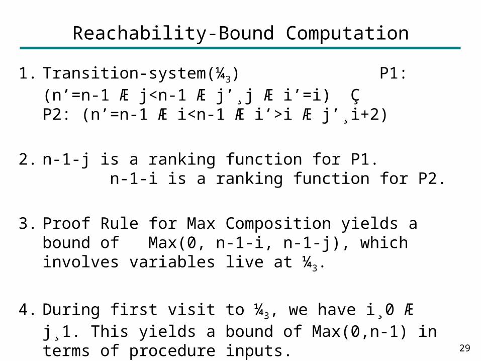
1. Transition-system(¼3) P1: (n’=n-1 Æ j<n-1 Æ j’¸j Æ i’=i) Ç

P2: (n’=n-1 Æ i<n-1 Æ i’>i Æ j’¸i+2)

2. n-1-j is a ranking function for P1. n-1-i is a ranking function for P2.

3. Proof Rule for Max Composition yields a bound of Max(0, n-1-i, n-1-j), which involves variables live at ¼3.

4. During first visit to ¼3, we have i¸0 Æ j¸1. This yields a bound of Max(0,n-1) in terms of procedure inputs.

29

Reachability-Bound Computation



proof rule based technique.• Loop has multiple paths.




Loop has other loops before it.– Perform backward symbolic execution (using proof


30


Visits(¼) = C3.Count · C1.Count

31

Backward Symbolic Execution (.Net Library)

Inputs: List<int> C1, List<int> C2

List<int> C3 = new List<int>();

AddElements(C3,C1); DeleteElements(C3,C2); ¼: foreach (int e in C3) … AddElements(List<int> L1, List<int>

L2) foreach (int e in L2) L1.Add(e);

• Backward Propagation may require tracing back across procedure calls and loops.

DeleteElements(List<int> L1, List<int> L2)

foreach (int e in L2) if (L1.Contains(e)) L1.Delete(e);

Use algorithm for computing Visits to relate values of a variable before and after a loop.

32

Backward Symbolic Execution across Loops

n := mwhile (e) { S1 ¼: n :=

n+3; S2}

nafter · nbefore + 3£Visits(¼)

• Computes symbolic computational complexity of procedures.

• Built over Phoenix Compiler Infrastructure and analyzes .Net binaries.

• Uses Z3 SMT solver as the logical reasoning engine.– Can reason about various data-types: arithmetic, bit-

vector, boolean, list/collection variables.• Takes between 0.1 to 1 second to analyze each loop.• Success ratio of 60-90% for computing loop bounds.• Representative failure cases:

– Lack of global invariant analysis.• for (i:=0; i<n; i := i+g);• for (i:=0; ig; i := i+1);

– Failure to resolve virtual method calls. 33

SPEED Tool

Limitations and potential Extensions• Worst-case bounds (as opposed to average bounds)

– Challenge: Requires modeling average/representative inputs.

– Use profiling/user-annotations to rule out exceptional paths.

• Static cost model for timing analysis– Challenge: Difficult to model low-level architectural

details like caches, pipelines. – Profiling may help generate a precise cost model.

• Imprecision (may generate higher bounds than possible)– Challenge: Undecidable problem in general.– Possible to generate proof of precision of bounds.

• Sequential Programs (as opposed to Concurrent programs)– Challenge: Variety of concurrent programming models;

scheduling policies; # of processors– Might be possible to model some of them.

34

• Detailed lecture notes available at http://www.cs.uoregon.edu/research/summerschool/summer09

• Bound computation using Recurrence Relations– Albert, Arenas, Genaim, Puebla, SAS ‘08

• Termination– Disjunctively well-founded ranking functions

• Cook, Podelski, Rybalchenko, PLDI 2006– Size-change abstraction

• Ben-Amran, CAV 2009• Worst Case Execution Time

– R. Wilhelm et.al., ACM TECS 2007

35

Related Work

• Bound Computation: An important application area that can leverage advances in static program analysis.

• An effective solution involved a variety of techniques for reasoning about loops/fixed-points.– Iterative techniques for summarizing inner loops.– Constraint-based techniques for ranking functions. – Proof-rule based technique for composition of ranking

functions and bound computation in terms of inputs.

• Several important/open/challenging problems.– Concurrent Procedures, Average-case Bounds

36

Conclusion

texpoint fonts used in emf. read the texpoint manual before you delete this box.: a a

Documents

loop headers

proof rules

inner loops

given bound

visits1 visits2visits1

new c j

multiple paths

control location