texas instruments ti-82 graphics calculator i.1 getting - cengage

Part I: Texas Instruments TI-82 Graphics Calculator

I.1 Getting started with the TI-82

I.1.1 Basics: Press the ON key to begin using your TI-82 calculator. If you need to adjust the display contrast, first press 2nd, then press and hold (the up arrow key) to lighten or (the down arrow key)to darken. As you press and hold or , an integer between 0 (lightest) and 9 (darkest) appears in theupper right corner of the display. When you have finished with the calculator, turn it off to conserve batterypower by pressing 2nd and then OFF.

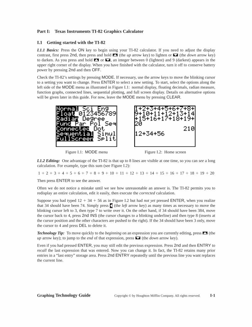
Check the TI-82’s settings by pressing MODE. If necessary, use the arrow keys to move the blinking cursorto a setting you want to change. Press ENTER to select a new setting. To start, select the options along theleft side of the MODE menu as illustrated in Figure I.1: normal display, floating decimals, radian measure,function graphs, connected lines, sequential plotting, and full screen display. Details on alternative optionswill be given later in this guide. For now, leave the MODE menu by pressing CLEAR.

Figure I.1: MODE menu Figure I.2: Home screen

I.1.2 Editing: One advantage of the TI-82 is that up to 8 lines are visible at one time, so you can see a longcalculation. For example, type this sum (see Figure I.2):

Then press ENTER to see the answer.

Often we do not notice a mistake until we see how unreasonable an answer is. The TI-82 permits you toredisplay an entire calculation, edit it easily, then execute the corrected calculation.

Suppose you had typed as in Figure I.2 but had not yet pressed ENTER, when you realizethat 34 should have been 74. Simply press (the left arrow key) as many times as necessary to move theblinking cursor left to 3, then type 7 to write over it. On the other hand, if 34 should have been 384, movethe cursor back to 4, press 2nd INS (the cursor changes to a blinking underline) and then type 8 (inserts atthe cursor position and the other characters are pushed to the right). If the 34 should have been 3 only, movethe cursor to 4 and press DEL to delete it.

Technology Tip: To move quickly to the beginning on an expression you are currently editing, press (theup arrow key); to jump to the end of that expression, press (the down arrow key).

Even if you had pressed ENTER, you may still edit the previous expression. Press 2nd and then ENTRY torecall the last expression that was entered. Now you can change it. In fact, the TI-82 retains many priorentries in a “last entry” storage area. Press 2nd ENTRY repeatedly until the previous line you want replacesthe current line.

12 � 34 � 56

1 � 2 � 3 � 4 � 5 � 6 � 7 � 8 � 9 � 10 � 11 � 12 � 13 � 14 � 15 � 16 � 17 � 18 � 19 � 20

Graphing Technology Guide Copyright © by Houghton Mifflin Company. All rights reserved. I-1

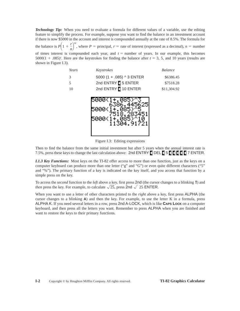
Technology Tip: When you need to evaluate a formula for different values of a variable, use the editingfeature to simplify the process. For example, suppose you want to find the balance in an investment accountif there is now $5000 in the account and interest is compounded annually at the rate of 8.5%. The formula for

the balance is where principal, rate of interest (expressed as a decimal), number

of times interest is compounded each year, and number of years. In our example, this becomesHere are the keystrokes for finding the balance after 5, and 10 years (results are

shown in Figure I.3).

Years Keystrokes Balance

3 5000 (1 + .085) ^ 3 ENTER $6386.45

5 2nd ENTRY 5 ENTER $7518.28

10 2nd ENTRY 10 ENTER $11,304.92

Figure I.3: Editing expressions

Then to find the balance from the same initial investment but after 5 years when the annual interest rate is7.5%, press these keys to change the last calculation above: 2nd ENTRY DEL 5 7 ENTER.

I.1.3 Key Functions: Most keys on the TI-82 offer access to more than one function, just as the keys on acomputer keyboard can produce more than one letter (“g” and “G”) or even quite different characters (“5”and “%”). The primary function of a key is indicated on the key itself, and you access that function by asimple press on the key.

To access the second function to the left above a key, first press 2nd (the cursor changes to a blinking ) andthen press the key. For example, to calculate press 2nd 25 ENTER.

When you want to use a letter of other characters printed to the right above a key, first press ALPHA (thecursor changes to a blinking A) and then the key. For example, to use the letter K in a formula, press ALPHA K. If you need several letters in a row, press 2nd A-LOCK, which is like CAPS LOCK on a computerkeyboard, and then press all the letters you want. Remember to press ALPHA when you are finished andwant to restore the keys to their primary functions.

� �25,

➞

t � 3,5000�1 � .085)t.t �

n �r �P �P�1 �rn�

nt

,

I-2 Copyright © by Houghton Mifflin Company. All rights reserved. TI-82 Graphics Calculator

I.1.4 Order of Operations: The TI-82 performs calculations according to the standard algebraic rules.Working outwards from inner parentheses, calculations are performed from left to right. Powers and rootsare evaluated first, followed by multiplications and divisions, and then additions and subtractions.

Note that the TI-82 distinguishes between subtraction and the negative sign. If you wish to enter a negativenumber, it is necessary to use (-) key. For example, you would evaluate by pressing (-) 5 – (4 (-) 3 ) ENTER to get 7.

Enter these expressions to practice using your TI-82.

Expression Keystrokes Display

7 – 5 3 ENTER -8

(7 – 5) 3 ENTER 6

120 – 10 ENTER 20

(120 – 10) ENTER 12100

24 ÷ 2 ^ 3 ENTER 3

(24 ÷ 2) ^ 3 ENTER 1728

(7 – (-) 5 ) (-) 3 ENTER -36

I.1.5 Algebraic Expressions and Memory: Your calculator can evaluate expressions such as after

you have entered a value for N. Suppose you want Press 200 STO ALPHA N ENTER to store

the value of 200 in memory location N. Whenever you use N in an expression, the calculator will substitute

the value 200 until you make a change by storing another number in N. Next enter the expression

by typing ALPHA N ( ALPHA N + 1 ) ÷ 2 ENTER. For you will find that

The contents of any memory location may be revealed by typing just its letter name and then ENTER. Andthe TI-82 retains memorized values even when it is turned off, so long as its batteries are good.

I.1.6 Repeated Operations with ANS: The result of your last calculation is always stored in memorylocation ANS and replaces any previous result. This makes it easy to use the answer from one computationin another computation. For example, press 30 + 15 ENTER so that 45 is the last result displayed. Thenpress 2nd ANS ÷ 9 ENTER and get 5 because

With a function like division, you press the key after you enter an argument. For such functions, wheneveryou would start a new calculation with the previous answer followed by pressing the function key, you maypress just the function key. So instead of 2nd ANS ÷ 9 in the previous example, you could have pressedsimply ÷ 9 to achieve the same result. This technique also works for these functions: + – .x -1�x2�

�

45 � 9 � 5.

N�N � 1�2

� 20,100.N � 200,

N�N � 1�2

�N � 200.

N�N � 1�2

��7 � �5� � �3

�242 �

3

2423

x 2�120 � 10�2

x 2120 � 102

��7 � 5� � 3

�7 � 5 � 3

�

�5 � (4 � �3)


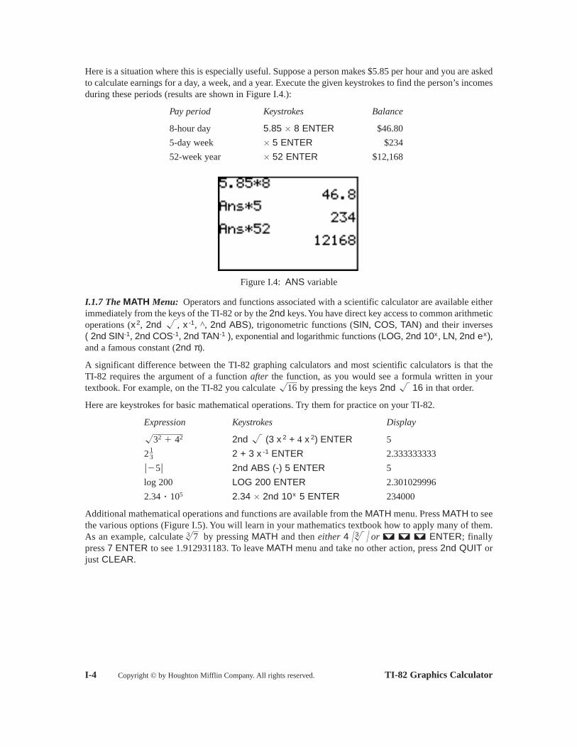
Here is a situation where this is especially useful. Suppose a person makes $5.85 per hour and you are askedto calculate earnings for a day, a week, and a year. Execute the given keystrokes to find the person’s incomesduring these periods (results are shown in Figure I.4.):

Pay period Keystrokes Balance

8-hour day 5.85 8 ENTER $46.80

5-day week 5 ENTER $234

52-week year 52 ENTER $12,168

Figure I.4: ANS variable

I.1.7 The MATH Menu: Operators and functions associated with a scientific calculator are available eitherimmediately from the keys of the TI-82 or by the 2nd keys. You have direct key access to common arithmeticoperations ( , 2nd , , ^, 2nd ABS), trigonometric functions (SIN, COS, TAN) and their inverses ( 2nd SIN , 2nd COS , 2nd TAN ), exponential and logarithmic functions (LOG, 2nd , LN, 2nd ),and a famous constant (2nd π).

A significant difference between the TI-82 graphing calculators and most scientific calculators is that the TI-82 requires the argument of a function after the function, as you would see a formula written in yourtextbook. For example, on the TI-82 you calculate by pressing the keys 2nd 16 in that order.

Here are keystrokes for basic mathematical operations. Try them for practice on your TI-82.


2nd (3 + 4 ) ENTER 5

2 + 3 ENTER 2.333333333

2nd ABS (-) 5 ENTER 5

log 200 LOG 200 ENTER 2.301029996

2.34 2nd 5 ENTER 234000

Additional mathematical operations and functions are available from the MATH menu. Press MATH to seethe various options (Figure I.5). You will learn in your mathematics textbook how to apply many of them.As an example, calculate by pressing MATH and then either 4 � � or ENTER; finallypress 7 ENTER to see 1.912931183. To leave MATH menu and take no other action, press 2nd QUIT orjust CLEAR.

3� 3�7

10x�2.34 � 105

�5x -121

3

x 2x 2� �32 � 42

� �16

ex10x-1-1-1x -1� x2

�

�

�


Figure I.5: MATH menu

The factorial of a nonnegative integer is the product of all the integers from 1 up to the given integer. Thesymbol for factorial is the exclamation point. So 4! (pronounced four factorial ) is Youwill learn more about applications of factorials in your textbook, but for now use the TI-82 to calculate 4!The factorial command is located in the MATH menu’s PRB sub-menu. to compute 4!, press thesekeystrokes: 4 MATH 4 ENTER or 4 MATH ENTER ENTER.

Note that you can select a sub-menu from the MATH menu by pressing either or . It is easier to press once than to press three times to get to the PRB sub-menu.

I.2 Functions and Graphs

I.2.1 Evaluating Functions: Suppose you received a monthly salary of $1975 plus a commission of 10% of sales. Let your sales in dollars; then your wages in dollars are given by the equation

If your January sales were $2230 and your February sales were $1865, what was your income during those months?

Here’s one method to use your TI-82 to perform this task. Press the Y= key at the top of the calculator todisplay the function editing screen (Figure I.6). You may enter as many as ten different functions for the TI-82 to use at one time. If there is already a function , press or as many times as necessary tomove the cursor to and then press CLEAR to delete whatever was there. Then enter the expression

by pressing these keys: 1975 + .10 X,T, . (The X,T, key lets you enter the variable X easilywithout having to use the ALPHA key.) Now press 2nd QUIT to return to the main calculations screen.

Figure I.6: Y= screen Figure I.7: Evaluating a function

��1975 � .10xY1

Y1

W � 1975 � .10x.Wx �

1 � 2 � 3 � 4 � 24.


Assign the value 2230 to the variable by using these keystrokes (see Figure I.7): 2230 STO X,T, .Then press 2nd : to allow another expression to be entered on the same command line. Next press thefollowing keystrokes to evaluate and find January’s wages: 2nd Y-VARS 1 [Function] 1 [ ] ENTER. Itis not necessary to repeat all these steps to find the February wages. Simply press 2nd ENTRY to recall theentire previous line, change 2230 to 1865, and press ENTER. Each time the TI-82 evaluates the function ,it uses the current value of

Figure I.8: Function notation

Like your textbook, the TI-82 uses standard function notation. So, to evaluate whenpress 2nd Y-VARS 1 1 (2230) ENTER (see Figure I.8). Then to evaluate

press 2nd ENTRY to recall the last line, change 2230 to 1865, and press ENTER.

You may also have the TI-82 make a table of values for the function. Press 2nd TblSet to set up the table(Figure I.9). Move the blinking cursor onto Ask beside Indpnt:, then press ENTER. This configurationpermits you to input values for one at a time. Now press 2nd TABLE, enter 2230 in the X column, andpress ENTER (see Figure I.10). Continue to enter additional values for X and the calculator automaticallycompletes the table with corresponding values of . Press 2nd QUIT to leave the TABLE screen.

Figure I.9: TblSet screen Figure I.10: Table of values

For a table containing values for 2, 3, 4, 5, and so on, set TblMin 1 to start at �Tbl 1 toincrement in steps of 1, and both Indpnt and Depend to Auto.

Technology Tip: The TI-82 does not require multiplication to be expressed between variables, so meansIt is often easier to press two or three ’s together than to search for the square key or the powers key. Of

course, expressed multiplication is also not required between a constant and variable. So, to enterin the TI-82, you might save keystrokes and press just these keys: 2 X,T, X,T,

X,T, + 3 X,T, X,T, 4 X,T, + 5.��2x3 � 3x2 � 4x � 5

xx3.xxx

�x � 1,�x � 1,

Y1

x

Y1�1865),Y1�x� � 1975 � .10x,Y1�2230�

x.Y1

Y1Y1

��x


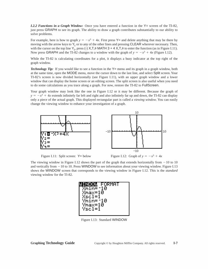
I.2.2 Functions in a Graph Window: Once you have entered a function in the Y= screen of the TI-82,just press GRAPH to see its graph. The ability to draw a graph contributes substantially to our ability tosolve problems.

For example, here is how to graph First press Y= and delete anything that may be there bymoving with the arrow keys to or to any of the other lines and pressing CLEAR wherever necessary. Then,with the cursor on the top line press (-) X,T, MATH 3 + 4 X,T, to enter the function (as in Figure I.11).Now press GRAPH and the TI-82 changes to a window with the graph of (Figure I.12).

While the TI-82 is calculating coordinates for a plot, it displays a busy indicator at the top right of the graph window.

Technology Tip: If you would like to see a function in the Y= menu and its graph in a graph window, bothat the same time, open the MODE menu, move the cursor down to the last line, and select Split screen. YourTI-82’s screen is now divided horizontally (see Figure I.11), with an upper graph window and a lowerwindow that can display the home screen or an editing screen. The split screen is also useful when you needto do some calculations as you trace along a graph. For now, restore the TI-82 to FullScreen.

Your graph window may look like the one in Figure I.12 or it may be different. Because the graph ofextends infinitely far left and right and also infinitely far up and down, the TI-82 can display

only a piece of the actual graph. This displayed rectangular part is called a viewing window. You can easilychange the viewing window to enhance your investigation of a graph.

Figure I.11: Split screen: Y= below Figure I.12: Graph of

The viewing window in Figure I.12 shows the part of the graph that extends horizontally from to 10and vertically from to 10. Press WINDOW to see information about your viewing window. Figure I.13shows the WINDOW screen that corresponds to the viewing window in Figure I.12. This is the standardviewing window for the TI-82.

Figure I.13: Standard WINDOW

�10�10

y � �x3 � 4x

10

−10

−10 10

y � �x3 � 4x

y � �x3 � 4x��Y1,

Y1

y � �x3 � 4x.


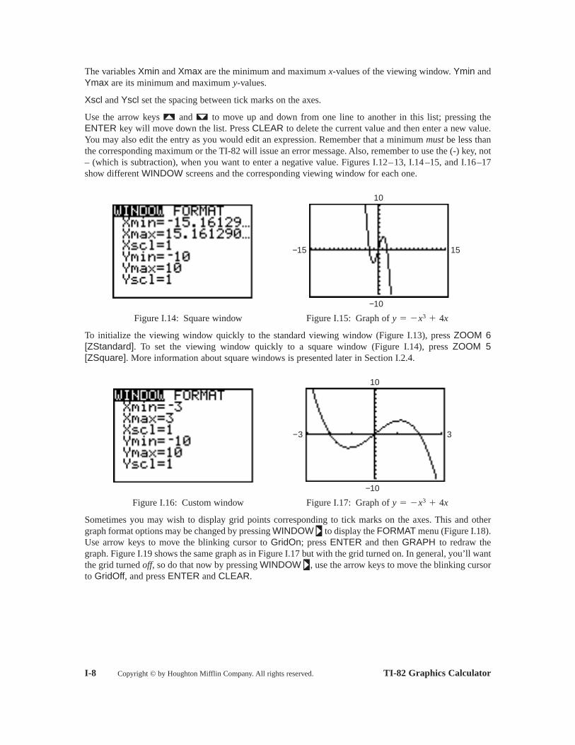
The variables Xmin and Xmax are the minimum and maximum values of the viewing window. Ymin andYmax are its minimum and maximum values.

Xscl and Yscl set the spacing between tick marks on the axes.

Use the arrow keys and to move up and down from one line to another in this list; pressing theENTER key will move down the list. Press CLEAR to delete the current value and then enter a new value.You may also edit the entry as you would edit an expression. Remember that a minimum must be less thanthe corresponding maximum or the TI-82 will issue an error message. Also, remember to use the (-) key, not– (which is subtraction), when you want to enter a negative value. Figures I.12–13, I.14 –15, and I.16–17show different WINDOW screens and the corresponding viewing window for each one.

Figure I.14: Square window Figure I.15: Graph of

To initialize the viewing window quickly to the standard viewing window (Figure I.13), press ZOOM 6[ZStandard]. To set the viewing window quickly to a square window (Figure I.14), press ZOOM 5[ZSquare]. More information about square windows is presented later in Section I.2.4.

Figure I.16: Custom window Figure I.17: Graph of

Sometimes you may wish to display grid points corresponding to tick marks on the axes. This and othergraph format options may be changed by pressing WINDOW to display the FORMAT menu (Figure I.18).Use arrow keys to move the blinking cursor to GridOn; press ENTER and then GRAPH to redraw thegraph. Figure I.19 shows the same graph as in Figure I.17 but with the grid turned on. In general, you’ll wantthe grid turned off, so do that now by pressing WINDOW , use the arrow keys to move the blinking cursorto GridOff, and press ENTER and CLEAR.

y � �x3 � 4x

10

−10

−3 3

y � �x3 � 4x

10

−10

−15 15

y-x-


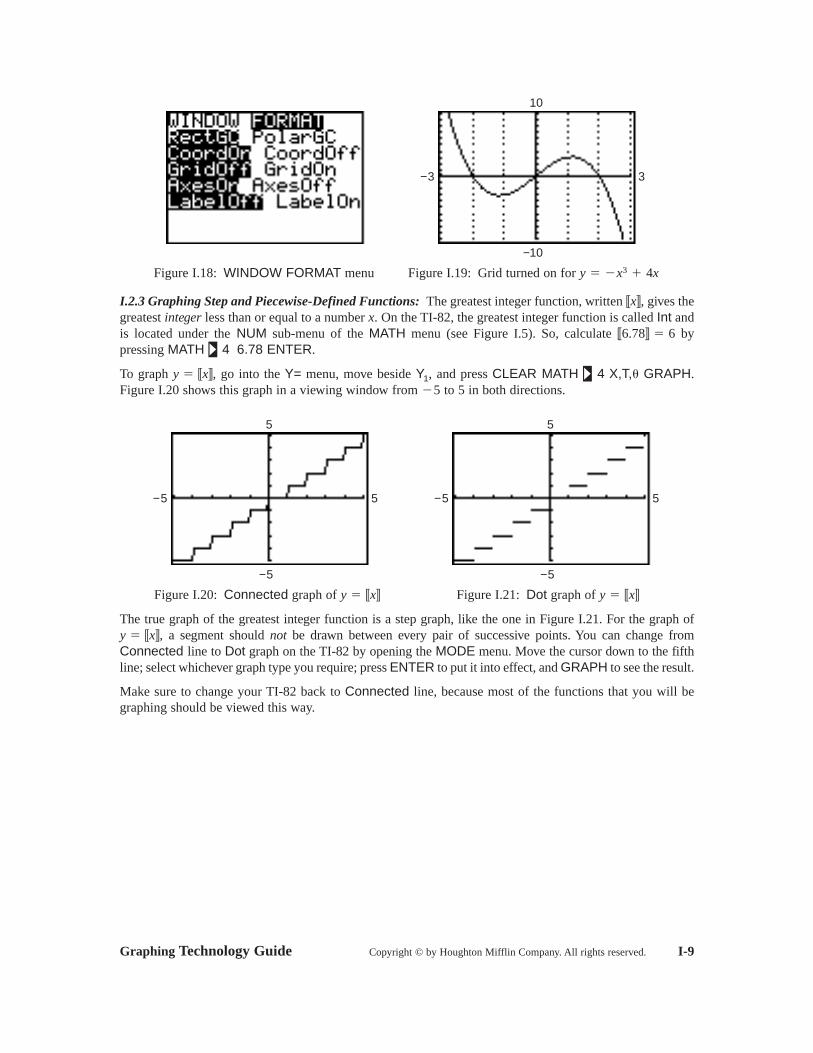
Figure I.18: WINDOW FORMAT menu Figure I.19: Grid turned on for

I.2.3 Graphing Step and Piecewise-Defined Functions: The greatest integer function, written gives thegreatest integer less than or equal to a number On the TI-82, the greatest integer function is called Int andis located under the NUM sub-menu of the MATH menu (see Figure I.5). So, calculate bypressing MATH 4 6.78 ENTER.

To graph go into the Y= menu, move beside and press CLEAR MATH 4 X,T, GRAPH.Figure I.20 shows this graph in a viewing window from to 5 in both directions.

Figure I.20: Connected graph of Figure I.21: Dot graph of

The true graph of the greatest integer function is a step graph, like the one in Figure I.21. For the graph ofa segment should not be drawn between every pair of successive points. You can change from

Connected line to Dot graph on the TI-82 by opening the MODE menu. Move the cursor down to the fifthline; select whichever graph type you require; press ENTER to put it into effect, and GRAPH to see the result.

Make sure to change your TI-82 back to Connected line, because most of the functions that you will begraphing should be viewed this way.

y � x�,

y � x�y � x�

5

−5

−5 5

5

−5

−5 5

�5�Y1,y � x�,

6.78� � 6x.

x�,

y � �x3 � 4x

10

−10

−3 3


The TI-82 can graph piecewise-defined functions by using the options in the TEST menu (Figure I.22) thatis displayed by pressing 2nd TEST. Each TEST function returns the value 1 if the statement is true, and thevalue 0 if the statement is false.

Figure I.22: 2nd TEST menu

For example, to graph the function (using Dot graph) enter the following keystrokes

Y= ( X,T, + 1) ( X,T, 2nd TEST 5 0 ) + ( X,T, – 1 ) ( X,T, 2nd TEST 4 0 ) (Figure I.23). Thenchange the mode to Dot graph and press GRAPH to display the graph. Figure I.24 shows this graph in aviewing window from to 5 in both directions.

Figure I.23: Piecewise-defined function Figure I.24: Piecewise-defined graph

I.2.4 Graphing a Circle: Here is a useful technique for graphs that are not functions, but that can be “split”into a top part and a bottom part, or into multiple parts. Suppose you wish to graph the circle whose equationis First solve for and get an equation for the top semicircle, and for thebottom semicircle, Then graph the two semicircles simultaneously.

Use the following keystrokes to draw the circle’s graph. Enter as and as (see Figure I.25) by pressing Y= CLEAR 2nd ( 36 X,T, ) ENTER CLEAR (-) 2nd

( 36 X,T, ). Then press GRAPH to draw them both.� x2�

� � x2�� Y2

��36 � x2Y1�36 � x2

y � ��36 � x2.y � �36 � x2,yx2 � y2 � 36.

5

−5

−5 5

�5

�� x2

f �x� � �x2 � 1,x � 1,

x < 0x ≥ 0


Figure I.25: Two semicircles Figure I.26: Circle’s graph – standard WINDOW

If your range were set to the standard viewing window, your graph would look like Figure I.26. Now thisdoes not look like a circle, because the units along the axes are not the same. This is where the squareviewing window is important. Press ZOOM 5 and see a graph that appears more circular.

Figure I.27: Figure I.28: A “square” circle

Technology Tip: Another way to get a square graph is to change the range variables so that the value ofYmax - Ymin is approximately times Xmax - Xmin. For example, see the WINDOW in Figure I.27 andthe corresponding graph in Figure I.28. This method works because the dimensions of the TI-82’s displayare such that the ratio of vertical to horizontal is approximately

The two semicircles in Figure I.28 do not connect because of an idiosyncrasy in the way the TI-82 plots a graph.

Back when you entered as and as you could have entered as and savedsome keystrokes. Try this by going back to the Y= menu and pressing to move the cursor down to Then press CLEAR (-) 2nd Y-VARS 1 1. The graph should be just as it was before.

I.2.5 TRACE: Graph from Section I.2.2 in the standard viewing window. (Remember toclear any other functions in the Y= screen.) Press any of the arrow keys , , , and see the cursormove from the center of the viewing window. The coordinates of the cursor’s location are displayed at thebottom of the screen, as in Figure I.29, in floating decimal format. This cursor is called a free-moving cursorbecause it can move from dot to dot anywhere in the graph window.

y � �x3 � 4x

Y2.Y2-Y1Y2,��36 � x2Y1�36 � x2

23.

23

verticalhorizontal

�1624

�23

8

−8

−12 12

10

−10

−10 10


Figure I.29: Free-moving cursor

Remove the free-moving cursor and its coordinates from the window by pressing GRAPH, CLEAR, orENTER. Press an arrow key again and the free-moving cursor will reappear at the same point you left it.

Figure I.30: TRACE

Press TRACE to enable the left and right arrow keys to move the cursor from point to point along thegraph of the function. The cursor is no longer free-moving, but is now constrained to the function. Thecoordinates that are displayed belong to points on the function’s graph, so the coordinate is the calculatedvalue of the function at the corresponding coordinate (Figure I.30).

Now plot a second function, along with Press Y=, move the cursor to the line,and enter then press GRAPH to see both functions.

Figure I.31: Two functions Figure I.32: and

Note in Figure I.31 that the equal signs next to and are both highlighted. This means both functionswill be graphed as shown in Figure I.32. In the Y= screen, move the cursor directly on top of the equal signnext to and press ENTER. This equal sign should no longer be highlighted (see Figure I.33). Now pressGRAPH and see that only is plotted (Figure I.34).Y2

Y1

Y2Y1

y � �.25xy � �x3 � 4x

10

−10

−10 10

�.25x,Y2y � �x3 � 4x.y � �.25x,

x-y-

10

−10

−10 10

10

−10

−10 10


Figure I.33: Y= screen with only active Figure I.34: Graph of

Many different functions can be stored in the Y= list and any combination of them may be graphedsimultaneously. You can make a function active or inactive for graphing by pressing ENTER on its equalsign to highlight (activate) or remove the highlight (deactivate). Now go back to the Y= screen and do whatis needed in order to graph but not

Now activate both functions so that both graphs are plotted. Press TRACE and the cursor appears first onthe graph of because it is higher up in the Y= list. You know that the cursor is on this function,

, because of the numeral 1 that is displayed in the upper right corner of the screen (see Figure I.30). Pressthe up or down arrow key to move the cursor vertically to the graph of Now the numeral2 is displayed in the upper right corner of the screen. Next press the left and right arrow keys to trace alongthe graph of When more than one function is plotted, you can move the trace cursor verticallyfrom one graph to another with the and keys.

Technology Tip: Trace along the graph of and press and hold either or . Eventually you willreach the left or right edge of the window. Keep pressing the arrow key and the TI-82 will allow you tocontinue the trace by panning the viewing window. Check the WINDOW screen to see that Xmin and Xmaxare automatically updated.

If you trace along the graph of the cursor will eventually move above or below the viewingwindow. The cursor’s coordinates on the graph will still be displayed, though the cursor itself can no longerbe seen. When you are tracing along a graph, press ENTER and the window will quickly pan over so thatthe cursor’s position on the function is centered in a new viewing window. This feature is especially helpfulwhen you trace near or beyond the edge of the current viewing window.

The TI-82’s display has 95 horizontal columns of pixels and 63 vertical rows. So when you trace a curveacross a graph window, you are actually moving from Xmin to Xmax in 94 equal jumps, each called You

would calculate the size of each jump to be . Sometimes you may want the jumps to

be friendly numbers like 0.1 or 0.25 so that, when you trace along the curve, the coordinates will beincremented by such a convenient amount. Just set your viewing window for a particular increment bymaking Xmax = Xmin For example, if you want Xmin and set Xmax

Likewise, set Ymax = Ymin 62 if you want the vertical increment to besome special

To center your window around a particular point, and also have a certain set Xmin = 47and Xmax Likewise, make Ymin and Ymax For example,to center a window around the origin with both horizontal and vertical increments of 0.25, set therange so that Xmin Xmax Ymin

and Ymax � 0 � 31 � 0.25 � 7.75.�7.75,� 0 � 31 � 0.25 �� 0 � 47 � 0.25 � 11.75,� 0 � 47 � 0.25 � �11.75,

�0, 0),� k � 31 � �y.� k � 31 � �y� h � 47 � �x.

� �x�h�x,�h, k),

�y.�y��5 � 94 � 0.3 � 23.2.

��x � 0.3,�5�� 94 � �x.�x

x-

Xmax � Xmin94

�x �

�x.

y � �x3 � 4x,

y � �.25x

y � �.25x.

y � �.25x.Y1

y � �x3 � 4x

Y2.Y1

y � �.25xY2

10

−10

−10 10


See the benefit by first graphing in a standard viewing window. Trace near its intercept,which is and move towards its intercept, which is Then press ZOOM 4 [ZDecimal] andtrace again near the intercepts.

I.2.6 ZOOM: Plot again the two graphs for and for There appears to be anintersection near The TI-82 provides several ways to enlarge the view around this point. You canchange the viewing window directly by pressing WINDOW and editing the values of Xmin, Xmax, Ymin,and Ymax. Figure I.36 shows a new viewing window for the range displayed in Figure I.35. The cursor hasbeen moved near the point of intersection; move your cursor closer to get the best approximation possiblefor the coordinates in the intersection.

Figure I.35: New WINDOW Figure I.36: Closer view

A more efficient method for enlarging the view is to draw a new viewing window with the cursor. Start againwith a graph of the two functions and in a standard viewing window (press ZOOM 6 for the standard window).

Now imagine a small rectangular box around the enter section point, near Press ZOOM 1 [ZBox](Figure I.37) to draw a box to define this new viewing window. Use the arrow keys to move the cursor, whosecoordinates are displayed at the bottom of the window, to one corner of the new viewing window you imagine.

Figure I.37: ZOOM menu Figure I.38: One corner selected

Press ENTER to fix the corner where you have moved the cursor; it changes shape and becomes a blinkingsquare (Figure I.38). Use the arrow keys again to move the cursor to the diagonally opposite corner of thenew rectangle (Figure I.39), then press ENTER. The rectangular area you have enclosed will now enlarge tofill the graph window (Figure I.40).

You may cancel the zoom any time before you press this last ENTER. Press ZOOM once more and startover. Press CLEAR or GRAPH to cancel the zoom, or press 2nd QUIT to cancel the zoom and return tothe home screen.

10

−10

−10 10

x � 2.

y � �.25xy � �x3 � 4x

2.5

−2.5

1.5 2.5

x � 2.y � �.25x.y � �x3 � 4x

��1, 0�.x-�0, 1�,y-y � x2 � 2x � 1


Figure I.39: Box drawn Figure I.40: New viewing window

You can also quickly magnify a graph around the cursor’s location. Return once more to the standard viewingwindow for the graph of the two functions and Press ZOOM 2 [Zoom In] andthen press arrow keys to move the cursor as close as you can to the point of intersection near (see Figure I.41). Then press ENTER and the calculator draws a magnified graph, centered at the cursor’sposition (Figure I.42). The range variables are changed to reflect this new viewing window. Look in theWINDOW menu to verify this.

Figure I.41: Before a zoom in Figure I.42: After a zoom in

As you see in the ZOOM menu (Figure I.37), the TI-82 can Zoom In (press ZOOM 2) or Zoom Out (pressZOOM 3). Zoom out to see a larger view of the graph, centered at the cursor position. You can change the horizontal and vertical scale of the magnification by pressing ZOOM 4 [SetFactors...] (see figure I.43)and editing XFact and YFact, the horizontal and vertical magnification factors (see Figure I.44).

The default zoom factor is 4 in both directions. It is not necessary for XFact and YFact to be equal.Sometimes, you may prefer to zoom in one direction only, so the other factor should be set to 1. As usual,press 2nd QUIT to leave the ZOOM menu.

Figure I.43: ZOOM MEMORY menu Figure I.44: ZOOM MEMORY SetFactors...

1.85

−3.15

−0.59 4.41

10

−10

−10 10

x � 2y � �.25x.y � �x3 � 4x

0.65

−1.29

1.49 2.77

10

−10

−10 10


Technology Tip: The TI-82 remembers the window it displayed before a zoom. So, if you should zoom intoo much and lose the curve, press ZOOM 1 [ZPrevious] to go back to the window before. If you want

to execute a series of zooms but then return to a particular window, press ZOOM 2 [ZoomSto] to store

the current window’s dimensions. Later, press ZOOM 3 [ZoomRcl] to recall the stored window.

I.2.7 Value: Graph in the standard viewing window (Figure I.12). The TI-82 can calculatethe value of this function for any given (between the Xmin and Xmax values).

Press 2nd CALC to display the CALCULATE menu (see Figure I.45), then press 1 [value]. The graph ofthe function is displayed and you are prompted to enter a value for Press 1 ENTER. The value youentered and its corresponding value are shown at the bottom of the screen and the cursor is located at thepoint on the graph (see Figure I.46).

Figure I.45: CALCULATE menu Figure I.46: Finding a value

Note that if you have more than one graph on the screen, the upper right corner of the TI-82 screen willdisplay the numeral corresponding to the equation of the function in the Y= list whose value is beingcalculated. Press the up or down arrow key to move the cursor vertically between functions at theentered value.

I.2.8 Relative Minimums and Maximums: Graph once again in the standard viewing win-dow (Figure I.12). This function appears to have a relative minimum near and a relative maximumnear 1. You may zoom and trace to approximate these extreme values.

First trace along the curve near the relative minimum. Notice by how much the values and values changeas you move from point to point. Trace along the curve until the coordinate is as small as you can get it,so that you are as close as possible to the relative minimum, and zoom in (press ZOOM 2 ENTER or use azoom box). Now trace again along the curve and, as you move from point to point, see that the coordinateschange by smaller amounts than before. Keep zooming and tracing until you find the coordinates of therelative minimum point as accurately as you need them, approximately

Figure I.47: Finding a minimum

10

−10

−10 10

��1.15, �3.08�.

y-y-x-

�xx � �1

y � �x3 � 4x

x-

10

−10

−10 10

�1, 3�y-

x-x.

xy � �x3 � 4x


Follow a similar procedure to find the relative maximum. Trace along the curve until the coordinate is asgreat as you can get it, so that you are as close as possible to the relative maximum, and zoom in. The relativemaximum point on the graph of is approximately

The TI-82 can automatically find the relative minimum and relative maximum points. Press 2nd CALC todisplay the CALCULATE menu (Figure I.45). Choose 3 [minimum] to calculate the minimum value of thefunction and 4 [maximum] for the maximum. You will be prompted to trace the cursor along the graph firstto a point left of the minimum/maximum (press ENTER to set this lower bound). Then move to a point rightof the minimum/maximum and set an upper bound and press ENTER. Note the two arrows at the top of thedisplay marking the lower and upper bounds (as in Figure I.47).

Next move the cursor along the graph between the two bounds and as close to the minimum/maximum asyou can; this serves as a guess for the TI-82 to start its search. Good choices for the lower bound, upperbound, and guess can help the calculator work more efficiently and quickly. Press ENTER and thecoordinates of the relative minimum/maximum point will be displayed (see Figure I.48).

Figure I.48: Relative minimum on

Note that if you have more than one graph on the screen, the upper right corner of the TI-82 screen willdisplay the numeral corresponding to the equation of the function in the Y= list whose minimum/maximumis being calculated.

I.2.9 Inverse Functions: The TI-82 draws the inverse function of a one-to-one function. Graph as in the standard viewing window (see Figure I.49). Next, press 2nd DRAW to display the DRAW menu.Use to move down and then choose 8 to draw the inverse function (see Figure I.50). Press 2nd Y-VARS

1 1 ENTER (see Figure I.51). These keystrokes instruct the TI-82 to draw the inverse function of . Theoriginal function and its inverse function will be displayed (see Figure I.52). Note that the calculator mustbe in function mode in order to use DrawInv.

To clear the graph of the inverse function, press 2nd DRAW 1 [ClrDraw].

Figure I.49: Graph of Figure I.50: DRAW menuy � x3 � 1

10

−10

−10 10

Y1

Y1

y � x3 � 1

y � �x3 � 4x

10

−10

−10 10

�1.15, 3.08�.y � �x3 � 4x

y-


Figure I.51: DrawInv Figure I.52: Graph of and its inverse function

I.2.10 Tangent Lines: Once again, graph in the standard viewing window (see Figure I.49). TheTI-82 can draw the tangent line to a graph of a function at a specified point.

While on the home screen, press 2nd DRAW 5 [Tangent(] 2nd Y-VARS 1 1 , 1 ) ENTER (see Figure I.53).These keystrokes instruct the TI-82 to draw the tangent line to the graph of at 1. The graph of theoriginal function and the tangent line to the graph at will be displayed (see Figure I.54).

To clear the tangent line, press 2nd DRAW 1.

Figure I.53: Tangent Figure I.54: Graph of and tangent line at

I.3 Solving Equations and Inequalities

I.3.1 Intercepts and Intersections: Tracing and zooming are also used to locate an intercept of a graph,where a curve crosses the axis. For example, the graph of crosses the axis three times (seeFigure I.55). After tracing over to the intercept point that is farthest to the left, zoom in (Figure I.56).Continue this process until you have located all three intercepts with as much accuracy as you need. Thethree intercepts of are approximately 0, and 2.828.

Figure I.55: Graph of Figure I.56: Near an intercept of y � x3 � 8xx-y � x3 � 8x

2.18

−2.82

−5.27 −0.27

10

−10

−10 10

�2.828,y � x3 � 8xx-

x-x-y � x3 � 8xx-x-

x � 1y � x3 � 1

10

−10

−10 10

x � 1x �Y1

y � x3 � 1

y � x3 � 1

10

−10

−10 10


Technology Tip: As you zoom in, you may also wish to change the spacing between tick marks on the axisso that the viewing window shows scale marks near the intercept point. Then the accuracy of yourapproximation will be such that the error is less than the distance between two tick marks. Change the scaleon the TI-82 from the WINDOW menu. Move the cursor down to Xscl and enter an appropriate value.

The intercept of a function’s graph is a root of the equation So press 2nd CALC to display theCALCULATE menu (Figure I.45) and choose 2 [root] to find a root of this function. Set a lower bound,upper bound, and guess as described in Section I.2.8. The TI-82 shows the coordinates of the point andindicates that it is a root (Figure I.57).

Figure I.57: A root of

TRACE and ZOOM are especially important for locating the intersection points of two graphs, say thegraphs of and Trace along one of the graphs until you arrive close to anintersection point. Then press or to jump to the other graph. Notice that the coordinate does notchange, but the coordinate is likely to be different (see Figures I.58 and I.59).

When the two coordinates are as close as they can get, you have come as close as you now can to the pointof intersection. so zoom in around the intersection point, then trace again until the two coordinates are asclose as possible. Continue this process until you have located the point of intersection with as much accu-racy as necessary. The points of intersection are approximately and

Figure I.58: Trace on Figure I.59: Trace on

You can also find the point of intersection of two graphs by pressing 2nd CALC 5 [intersect]. Trace withthe cursor first along one graph near the intersection and press ENTER; then trace with the cursor along theother graph and press ENTER. Marks are placed on the graphs at these points. Finally, move the cursornear the point of intersection and press ENTER again. Coordinates of the intersection will be displayed atthe bottom of the window. More will said about the intersect feature in Section I.3.3.

�

y � �.25xy � �x3 � 4x

3.2

−3.2

−4.7 4.7

3.2

−3.2

−4.7 4.7

�2.062, 0.515�.�0, 0�,��2.062, 0.515�,

y-y-

y-x-

y � �.25x.y � �x3 � 4x

y � x3 � 8x

10

−10

−10 10

f �x� � 0.x-

x-

x-


I.3.2 Solving Equations by Graphing: Suppose you need to solve the equation Firstgraph in a window large enough to exhibit all its intercepts, corresponding to all theequation’s real roots. Then use zoom and trace, or the TI-82’s roots finder, to locate each one. In fact, thisequation has just one real solution,

Remember that when an equation has more than one intercept, it may be necessary to change the viewingwindow a few times to locate all of them.

Technology Tip: To solve an equation like you may first rewrite it in general form,and proceed as above. However, you may also graph the two functions

and then zoom and trace to locate their point of intersection.

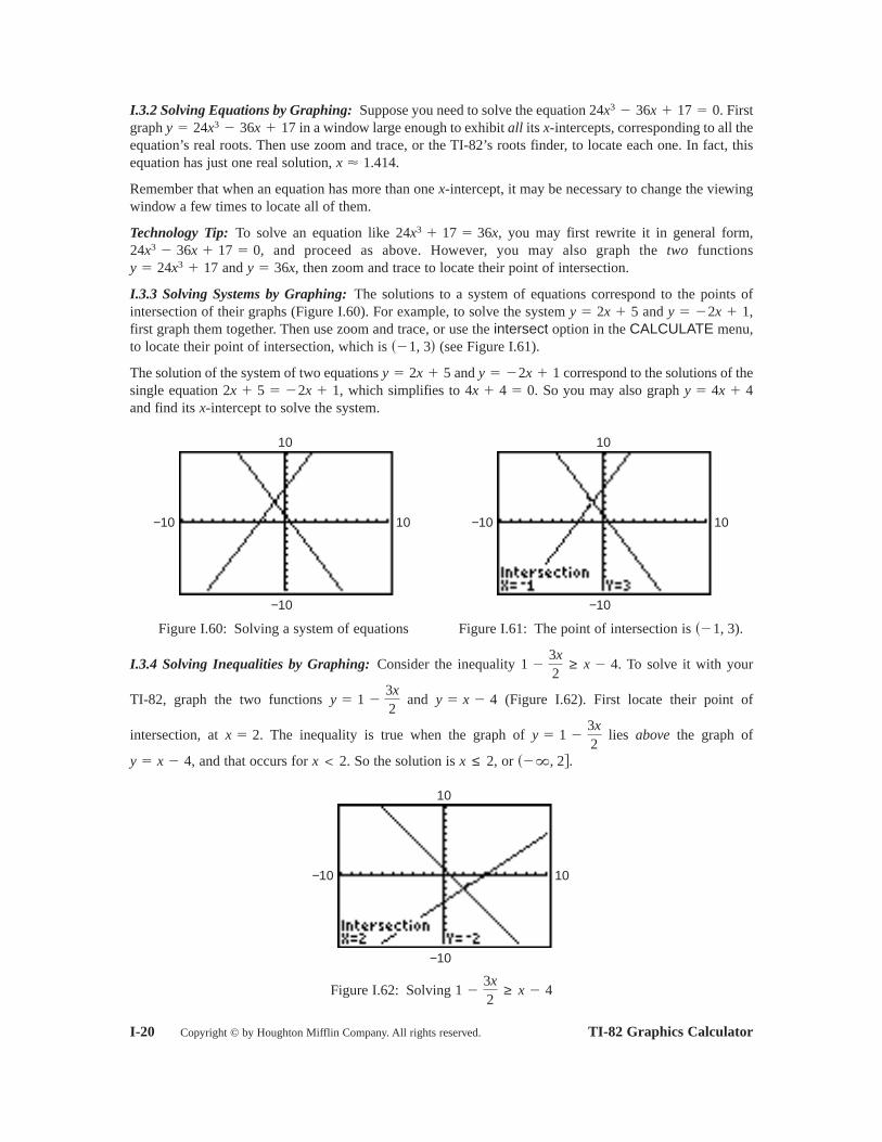
I.3.3 Solving Systems by Graphing: The solutions to a system of equations correspond to the points ofintersection of their graphs (Figure I.60). For example, to solve the system and first graph them together. Then use zoom and trace, or use the intersect option in the CALCULATE menu,to locate their point of intersection, which is (see Figure I.61).

The solution of the system of two equations and correspond to the solutions of thesingle equation which simplifies to So you may also graph and find its intercept to solve the system.

Figure I.60: Solving a system of equations Figure I.61: The point of intersection is

I.3.4 Solving Inequalities by Graphing: Consider the inequality To solve it with your

TI-82, graph the two functions and (Figure I.62). First locate their point of

intersection, at The inequality is true when the graph of lies above the graph of

and that occurs for So the solution is or

Figure I.62: Solving 1 �3x2

≥ x � 4

10

−10

−10 10

��, 2 .x ≤ 2,x < 2.y � x � 4,

y � 1 �3x2

x � 2.

y � x � 4y � 1 �3x2

1 �3x2

≥ x � 4.

��1, 3).

10

−10

−10 10

10

−10

−10 10

x-y � 4x � 44x � 4 � 0.2x � 5 � �2x � 1,

y � �2x � 1y � 2x � 5

��1, 3�

y � �2x � 1,y � 2x � 5

y � 36x,y � 24x3 � 1724x3 � 36x � 17 � 0,

24x3 � 17 � 36x,

x-

x � 1.414.

x-y � 24x3 � 36x � 1724x3 � 36x � 17 � 0.


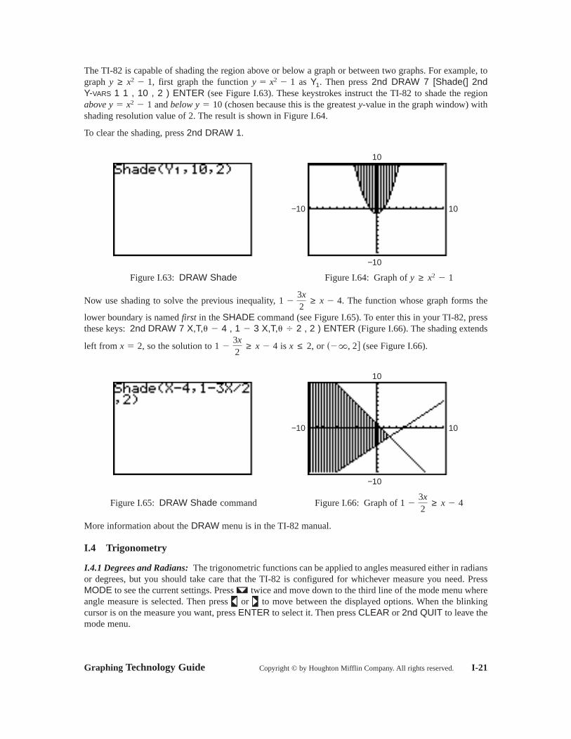
The TI-82 is capable of shading the region above or below a graph or between two graphs. For example, tograph first graph the function as . Then press 2nd DRAW 7 [Shade(] 2nd Y-VARS 1 1 , 10 , 2 ) ENTER (see Figure I.63). These keystrokes instruct the TI-82 to shade the regionabove and below (chosen because this is the greatest value in the graph window) withshading resolution value of 2. The result is shown in Figure I.64.

To clear the shading, press 2nd DRAW 1.

Figure I.63: DRAW Shade Figure I.64: Graph of

Now use shading to solve the previous inequality, The function whose graph forms the

lower boundary is named first in the SHADE command (see Figure I.65). To enter this in your TI-82, pressthese keys: 2nd DRAW 7 X,T, 4 , 1 3 X,T, 2 , 2 ) ENTER (Figure I.66). The shading extends

left from so the solution to is or (see Figure I.66).

Figure I.65: DRAW Shade command Figure I.66: Graph of

More information about the DRAW menu is in the TI-82 manual.

I.4 Trigonometry

I.4.1 Degrees and Radians: The trigonometric functions can be applied to angles measured either in radiansor degrees, but you should take care that the TI-82 is configured for whichever measure you need. PressMODE to see the current settings. Press twice and move down to the third line of the mode menu whereangle measure is selected. Then press or to move between the displayed options. When the blinkingcursor is on the measure you want, press ENTER to select it. Then press CLEAR or 2nd QUIT to leave themode menu.

1 �3x2

≥ x � 4

10

−10

−10 10

��, 2 x ≤ 2,1 �3x2

≥ x � 4x � 2,

��

1 �3x2

≥ x � 4.

y ≥ x2 � 1

10

−10

−10 10

y-y � 10y � x2 � 1

Y1y � x2 � 1y ≥ x2 � 1,


It’s a good idea to check the angle measure setting before executing a calculation that depends on a particularmeasure. You may change a mode setting at any time and not interfere with pending calculations. Try thefollowing keystrokes to see this in action.


sin 45 MODE ENTER CLEARSIN 45 ENTER .7071067812

sin SIN 2nd ENTER .0548036651

sin MODE ENTERCLEAR SIN 2ND ENTER 0

sin 45 SIN 45 ENTER .8509035245

sin SIN ( 2nd ÷ 6 ) ENTER .5

The first line of keystrokes sets the TI-82 in degree mode and calculates the sine of 45 degrees. While thecalculator is still in degree mode, the second line of keystrokes calculates the sine of degrees, Thethird line changes the radian mode just before calculating the sine of radians. The fourth line calculates

the sine of 45 radians. Finally, the fifth line calculates the sine of radians (the calculator remains in

radian mode).

The TI-82 makes it possible to mix degrees and radians in a calculation. Execute these keystrokes to calculate

as shown in Figure I.67. TAN 45 2nd ANGLE 1 [ ° ] + SIN ( 2nd ÷ 6 ) 2nd ANGLE

3 [ r ] ENTER. Do you get 1.5 whether your calculator is set either in degree mode or in radian mode?

Figure I.67: Angle measure

I.4.2 Graphs of Trigonometric Functions: When you graph a trigonometric function, you need to paycareful attention to the viewing window and to your angle measure configuration. For example, graph

in the standard viewing window in radian mode. Trace along the curve to see where it is. Zoom

in to a better window, or use the period and amplitude to establish better WINDOW values.

Technology Tip: Because when in radian mode, set and to cover theinterval from 0 to 2.

� 6.3Xmax� 0Xmin � 3.1,

y �sin 30x

30

tan 45� � sin

6

6

3.1415�.

6

�

�


Next graph in the standard window first, then press ZOOM 7 [ZTrig] to change to a special

window for trigonometric functions in which the Xscl is or and the vertical range is from

to 4. The TI-82 plots consecutive points and then connects them with a segment, so the graph is notexactly what you should expect. You may wish to change from Connected line to Dot graph (see Section I.2.3)when you plot the tangent function.

I.5 Scatter Plots

I.5.1 Entering Data: This table shows total prize money (in millions of dollars) awarded at the Indianapolis500 race from 1995 to 2003. (Source: Indy Racing League)

We’ll now use the TI-82 to construct a scatter plot that represents these points and to find a linear model thatapproximates the given data.

The TI-82 holds data in up to six lists. Before entering this new data, press STAT 4 [ClrList] 2nd L1, 2ndL2 , 2nd L3 , 2nd L4 , 2nd L5 , 2nd L6 ENTER to clear all data lists. This can also be done from withinthe list editor by highlighting each list title (L1, etc) and pressing CLEAR ENTER.

Now press STAT 1 [Edit] to reach the list editor. Instead of entering the full year, let represent 1995,represent 1996, and so on. Here are the keystrokes for the first three years: 5 ENTER 6 ENTER

7 ENTER and so on, then press to move to the first element of the next list and press 8.06 ENTER 8.11ENTER 8.61 ENTER and so on (see Figure I.68). Press 2nd QUIT when you have finished.

Figure I.68: Entering data points

You may edit statistical data in the same way you edit expressions in the home screen. Move the cursor toany value you wish to change, then type the correction. To insert or delete data, move the cursor over thedata point you wish to add or delete. Press 2nd INS and a new data point is created; press DEL and the datapoint is deleted.

I.5.2 Plotting Data: Once all the data points have been entered, press to display the Plot1

screen. Press ENTER to turn Plot1 on, select the other options shown in figure I.69, and press GRAPH.(Make sure that you have cleared or turned off any functions in the Y= screen, or those functions will begraphed simultaneously.) Figure I.70 shows this plot in a window from 0 to 15 in both directions. You maynow press TRACE to move from data point to data point.

2nd STATPLOT

1

x � 6x � 5

�4

90�

2� 1.5708

y � tan x


Year 1995 1996 1997 1998 1999 2000 2001 2002 2003

Prize (in millions) $8.06 $8.11 $8.61 $8.72 $9.05 $9.48 $9.61 $10.03 $10.15

Figure I.69: Plot1 menu Figure I.70: Scatter plot

To draw the scatter plot in a window adjusted automatically to include all the data you entered, pressZOOM 9 [ZoomStat].

When you no longer want to see the scatter plot, press , move the cursor to OFF, and press

ENTER. The TI-82 still retains all the data you entered.

I.5.3 Regression Line: The TI-82 calculates the slope and intercept for the line that best fits all the data.The TI-82 can calculate regression lines in two equivalent forms. After the data points have been entered,press STAT 5 [LinReg(ax + b)] ENTER to calculate a linear regression model with the slope named aand the intercept named b (Figure I.71). By pressing STAT 9 [LinReg(a + bx)] ENTER, the TI-82produces a linear regression model with the roles of a and b reversed. The number r (between and 1) iscalled the correlation coefficient and measures how well the linear regression equation fits the data. Thecloser is to 1, the better the fit; the closer is to 0, the worse the fit.

Turn Plot1 on again, if it is not currently displayed. Graph the regression line by pressing Y=,inactivating any existing functions, moving to a free line or clearing one, then pressing VARS 5 [Statistics...]

7 [RegEQ] GRAPH. See how well this line fits with your data points (Figure I.72).

Figure I.71: Linear regression model Figure I.72: Linear regression line

I.5.4 Other Regression Models: After data points have been entered, you can choose from seven differentregression models. They are all located in the CALC sub-menu of the STAT menu.

15

00 15

y � ax � b

rr

�1y-

y-

2nd STATPLOT

1

15

00 15


I.6 Matrices

I.6.1 Making a Matrix: The TI-82 can display and use five different matrices (A through E). Here’s how to

store this matrix in your calculator.

Press MATRX to see the matrix menu (Figure I.73); then press or just to switch to the matrix EDITmenu. Whenever you enter the matrix EDIT menu, the cursor starts at the top matrix. Move to another matrixby repeatedly pressing . For now, press ENTER to edit matrix

The display will show the dimension of matrix if the matrix exists; otherwise, it will display Change the dimensions of matrix to by pressing 3 ENTER 4 ENTER. Simply press ENTER oran arrow key to accept an existing dimension. The matrix shown in the window changes in size to reflect achanged dimension.

Figure I.73: MATRX menu Figure I.74: Editing a matrix

Use the arrow keys or press ENTER repeatedly to move the cursor to a matrix element you want to change.If you press ENTER, you will move right across a row and then back to the first column of the next row. Atthe right edge of the screen in Figure I.74, there are dashes to indicate more columns than are shown. Go tothem by pressing as many times as necessary. The ordered pair at the bottom left of the screen show thecursor’s current location withing the matrix. The element in the second row and first column in Figure I.74is highlighted, so the ordered pair at the bottom of the window is 2 , 1, and the screen shows that element’scurrent value. Continue to enter all the elements of matrix press ENTER after inputting each value.

When you are finished, leave the matrix editing screen by pressing 2nd QUIT to return to the home screen.

I.6.2 Matrix Math: From the home screen you can perform many calculations with matrices. To see matrixpress MATRX 1 ENTER (Figure I.75).

Perform the scalar multiplication 2 by pressing 2 MATRX 1 ENTER. The resulting matrix is displayedon the screen. To replace matrix by 2 press 2 MATRX 1 STO MATRX 2 ENTER (see FigureI.76), or if you do this immediately after calculating press only STO MATRX 2 ENTER. PressMATRX 2 to verify that the dimensions and entries of matrix have been changed automatically toreflect these new values.

�B �2�A ,

��A ,�B �A

�A ,

�A ;

3 � 4�A 1 � 1.�A

�A .

�1

�12

�23

�5

305

94

17�3 � 4


Figure I.75: Matrix Figure I.76: Matrix

Add the two matrices say and , create (with the same dimensions as ) and then press MATRX

1 MATRX 2 ENTER. Subtraction is performed in a similar manner. Now set the dimensions of matrix

to and enter the matrix: as For matrix multiplication of by press

MATRX 3 MATRX 1 ENTER. If you tried to multiply by your TI-82 would signal an errorbecause the dimensions of the two matrices do not permit multiplication in this way.

I.6.3 Row Operations: Here are the keystrokes necessary to perform elementary row operations on a matrix.Your textbook provides more careful explanation of the elementary row operations and their uses.

To interchange the second and third rows of the matrix that was defined in Figure I.75, press MATRX 8 [rowSwap( ] MATRX 1 , 2 , 3 ) ENTER (see Figure I.77). The format of this command isrowSwap(matrix, row1, row 2).

To add row 2 and row 3 and store the results in row 3, press MATRX 9 [row + ( ] MATRX 1 , 2 , 3 )ENTER. The format of this command is row+(matrix, row1, row2).

To multiply row 2 by and store the results in row 2, thereby replacing row 2 with new values, pressMATRX 0 [*row( ] (-) 4 , MATRX 1 , 2 ) ENTER. The format of this command *row(scalar,matrix, row ).

Figure I.77: Interchange rows 2 and 3 Figure I.78: Add times row 2 to row 3

To multiply row 2 by and add the results to row 3, thereby replacing row 3 with new values, pressMATRX ALPHA A [*row + (] (-) 4 , MATRX 1 , 2 , 3 ) ENTER (see Figure I.78). The format of thiscommand is *row+(scalar, matrix, row1, row2).

Technology Tip: Note that your TI-82 does not store a matrix obtained as the result of any row operations.So when you need to perform several row operations in succession, it is a good idea to store the result ofeach one in a temporary place. You may wish to use matrix to hold such intermediate results.

For example, use elementary row operations to solve this system of linear equations: � x � 2y�x � 3y2x � 5y

� 3z �

�

� 5z �

9�417

.

�E

�4

�4

�4

�A

�C ,�A �

�A ,�C �C .�21

0�5

3�1�2 � 3�C

�

�A �B �B �A

�B �A


First enter this augmented matrix as in your TI-82 : Next store this matrix in

(press MATRX 1 STO MATRX 5 ENTER) so you may keep the original in case you need to recall it.

Here are the row operations and their associated keystrokes. At each step, the result is stored in andreplaces the previous matrix The matrix in row-echelon form is shown in Figure I.79.

Row Operation Keystrokes

Add row 1 to row 2. MATRX 9 MATRX 5 , 1 , 2 )STO MATRX 5 ENTER

Add times row 1 to row 3. MATRX ALPHA A (-) 2 , MATRX 5 , 1 , 3 )STO MATRX 5 ENTER

Add row 2 to row 3. MATRX 9 MATRX 5 , 2 , 3 )STO MATRX 5 ENTER

Multiply row 3 by MATRX 0 1 ÷ 2 , MATRX 5 , 3 )STO MATRX 5 ENTER

Figure I.79: Row-echelon form of matrix after row operations

So, and

I.6.4 Determinants and Inverses: Enter this square matrix as To calculate its

determinant go to the home screen and press MATRX 1 [det] MATRX 1 ENTER.

You should find that the determinant is 2, as shown in Figure I.80.

Because the determinant of the matrix is not zero, it has an inverse, Press MATRX 1 ENTER tocalculate the inverse of matrix , also shown in Figure I.80.

Now let’s solve a system of linear equations by matrix inversion. Once more, consider

The coefficient matrix for this system is the matrix that was entered as matrix in the

previous example.

�A �1

�12

�23

�5

305�,

� x � 2y�x � 3y2x � 5y

� 3z �

�

� 5z �

9�417

.

�A x -1�A -1.

1�1

2

�23

�5

305,

�1

�12

�23

�5

305�.�A :3 � 3

x � 1.y � �1,z � 2,

�

12.

�

�

�2

�

�E .�E

��E

�1

�12

�23

�5

305

9�417�.�A


Figure I.80: and Figure I.81: Solution matrix

Now enter the matrix as Then press MATRX 1 MATRX 2 ENTER to calculate the

solution matrix (Figure I.81). The solution is still and

I.7 Sequences

I.7.1 Iteration with ANS Key: The ANS feature permits you to perform iteration, the process of evaluating

a function repeatedly. As an example, calculate for Then calculate for the answer

to the previous calculation. Continue to use each answer as in the next calculation. Here are keystrokes toaccomplish this iteration on TI-82 calculator (see the results in Figure I.82). Notice that when you use ANSin place of in a formula, it is sufficient to press ENTER to continue an iteration.

Iteration Keystrokes Display

1 27 ENTER 27

2 ( 2nd ANS 1 ) 3 ENTER 8.666666667

3 ENTER 2.555555556

4 ENTER .5185185185

5 ENTER -.1604938272

Figure I.82: Iteration

Press ENTER several more times and see what happens with this iteration. You may wish to try it again witha different starting value.

I.7.2 Terms of Sequences: Another way to display the terms of a sequence is to enter the sequence and thenumber of terms you want listed. For example, to find the first five terms of the sequence press 2nd LIST 5 [seq( ] (-) ALPHA N + 4, ALPHA N , 1 , 5 , 1 ) ENTER (see Figure I.83). The formatof this command is seq(expression, variable, begin, end, increment ).

un � �n � 4,

��

n

n

n �n � 1

3n � 27.

n � 13

z � 2.y � �1,x � 1,

�x -1�B .�9

�417�3 � 1

�A -1�A


Figure I.83: Terms of sequence

I.7.3 Arithmetic and Geometric Sequences: Use iteration with the ANS variable to determine the termof a sequence. For example, find the 18th term of an arithmetic sequence whose first term is 7 and whosecommon difference is 4. Enter the first term 7, then start the progression with the recursion formula,2nd ANS4 ENTER. This yields the 2nd term, so press ENTER sixteen more times to find the 18th term,75. For a geometric sequence whose common ration is 4, start the progression with 2nd ANS 4 ENTER.

You can also define the sequence recursively with the TI-82 by selecting Seq in the MODE menu (seeFigure I.1). Once again, let’s find the 18th term of an arithmetic sequence whose first term is 7 and whosecommon difference is 4. Press Mode ENTER 2nd QUIT. Then press Y= to edit eitherthe TI-82’s two sequences, and Make by pressing 2nd + 4. Now make by pressing WINDOW and setting UnStart = 7 and nStart = 1 (because the first term is where ).Press 2nd QUIT to leave this menu and return to the home screen. To find the 18th term of this sequence,calculate by pressing 2nd Y-VARS 4 1 ( 18 ) ENTER (see Figure I.84).

Figure I.84: Sequence mode

Of course, you could use the explicit formula for the term of an arithmetic sequence,First enter values for the variables and then evaluate the formula by pressing ALPHA A + ( ALPHA N 1 ) ALPHA D ENTER. For a geometric sequence whose term is given by enter values for the variables and then evaluate the formula by pressing ALPHA A ALPHA R ^ ( ALPHA N 1 ) ENTER.

To use the explicit formula in Seq MODE, make by pressing Y= and then 7 + ( 2nd n 1 ) 4 ENTER 2nd QUIT. Once more, calculate by pressing 2nd Y-VARS 4 1 ( 18 ) ENTER.

There are more instructions for using sequence mode in the TI-82 manual.

I.7.4 Sums of Sequences: You can find the sum of a sequence by combining the sum feature on the MATHsub-menu of the LIST menu with the seq( feature on the OPS sub-menu of the LIST menu. The format ofthe sum command is sum list, start, end, where the optional arguments start and end determine whichelements of list are summed. The format of the seq( command is seq(expression, variable, begin, end,increment ), where the argument increment indicates the difference between successive points at whichexpression is evaluated.

u18��un � 7 � �n � 1� � 4

�n,r,a,

tn � a � rn�1,nth�n,d,a,

tn � a � �n � 1�d.nth

u18

n � 1u1

u1 � 7Un -1un � un�1 � 4Vn.Un

�

nth

un � �n � 4


For example, suppose you want to find the sum Press 2nd LIST 5 [sum] 2nd LIST 5 [seq(]

4 ( .3 ) ^ ALPHA N , ALPHA N , 1 , 12 , 1 ) ENTER (Figure I.85). Note that the sum command doesnot need a starting or ending point, because every term in the sequence is being summed. Also, any letter canbe used for the variable in the sum, i.e., the N could just have easily been an A or a K.

Now calculate the sum starting at by using 2nd ENTRY to edit the starting value. You should obtaina sum of approximately 5.714284803.

Figure I.85:

I.8 Parametric and Polar Graphs

I.8.1 Graphing Parametric Equations: The TI-82 plots up to six pairs of parametric equations as easily asit plots functions. In the MODE menu (Figure I.1), go to the fourth line from the top, and change the settingto Par. Be sure, if the independent parameter is an angle measure, that the angle measure in the MODE menuis set to whichever you need, Radian or Degree.

For example, here are the keystrokes needed to graph the parametric equations and First check that angles are currently being measured in radians and change to parametric mode. Then pressY = ( COS X,T, ) ^ 3 ENTER ( SIN X,T, ) ^ 3 ENTER (Figure I.86). Note that when you press thevariable key X,T, you get a T because the calculator is in parametric mode.

Figure I.86: Parametric Y= menu Figure I.87: Parametric WINDOW menu

Press WINDOW to set the graphing window and to initialize the values of T. In the standard window, the

values of T go from 0 to in steps of with the view from to 10 in both directions. In

order to provide a better viewing window, press ENTER three times to move the cursor down, then set thewindow to extend from to 2 in both directions (Figure I.87). Press GRAPH to see the parametric graph(Figure I.88).

�2

�10

24� 0.1309,2

��

y � sin3 t.x � cos3 t

�12

n�14�0.3�n

n � 0

�12

n�14�0.3�n.


Figure I.88: Parametric graph of and

You may ZOOM and TRACE along parametric graphs just as you did with function graphs. However, unlikewith function graphs, the cursor will not move to values outside of the T range, so the left arrow will not

work when T and the right arrow will not work when T As you trace along this graph, noticethat the cursor moves in the counterclockwise direction as T increases.

I.8.2 Rectangular-Polar Coordinate Conversion: The 2nd ANGLE menu provides functions forconverting between rectangular and polar coordinate systems. These functions use the current angle measuresetting, so it is a good idea to check the default angle measure before any conversion. Of course, you mayoverride the current angle measure setting, as explained in Section I.4.1. For the following examples, the TI-82 is set to radian measure.

Given the rectangular coordinates convert from these rectangular coordinates to polarcoordinates by pressing 2nd ANGLE 5 [R �Pr(] 4 , (-) 3 ) ENTER to display the value of Nowpress 2nd ANGLE 6 [R � P (] 4 , (-) 3 ) ENTER to display the value of (see Figure I.89).

Figure I.89: Rectangular to polar coordinates Figure I.90: Polar to rectangular coordinates

Suppose To convert from these polar coordinates to rectangular coordinates press 2ndANGLE 7 [P � Rx(] 3 , 2nd ) ENTER to display the coordinate. Now press 2nd ANGLE 8 [P � Ry(]3 , 2nd ) ENTER to display the coordinate (see Figure I.90).

I.8.3 Graphing Polar Equations: The TI-82 graphs polar functions in the form In the fourth lineof the MODE menu, select Pol for polar graphs. You may now graph up to six different polar functions at atime. Be sure that the angle measure has been set to whichever you need, Radian or Degree. Here we willuse radian measure.

For example, to graph press Y= for the polar graph editing screen. Then enter the expressionfor r1 by pressing 4 SIN X,T, Note that when you press the variable key X,T, you get a because

the calculator is in polar mode (see Figure I.91). Choose a good viewing window and an appropriate intervaland increment for In Figure I.92, the viewing window is roughly “square” and extends from and 6horizontally and from to 4 vertically.�4

�6�.

��,�.4 sin �r � 4 sin �,

r � f ��.

y-x-

�x, y�,�r, �� 3, �.

��r.�r, ��

�x, y� � �4, �3�,

� 2.� 0,

y � sin3 tx � cos3 t

2

−2

−2 2


Figure I.91: Polar Y= menu Figure I.92: Polar graph of

Figure I.92 shows rectangular coordinates of the cursor’s location on the graph. You may sometimes wish totrace along the curve and see polar coordinates of the cursor’s location. The first line of the WINDOWFORMAT menu (Figure I.18) has options for displaying the cursor’s position in rectangular (RectGC) orpolar (PolarGC) form.

I.9 Probability and Statistics

I.9.1 Random Numbers: The command rand generates a number between 0 and 1. You will find thiscommand in the PRB (probability) sub-menu of the MATH menu. Press MATH 1 [rand] ENTER togenerate a random number. Press ENTER to generate another number; keep pressing ENTER to generatemore of them.

If you need a random number between, say, 0 and 10, then press 10 MATH 1 ENTER. To get a randomnumber between 5 and 15, press 5 + 10 MATH 1 ENTER.

I.9.2 Permutations and Combinations: To calculate the number of permutations of 12 objects taken 7 at atime, press 12 MATH 2 [nPr] 7 ENTER. So, as shown in Figure I.93.

Figure I.93: and

For the number of combinations of 12 objects taken 7 at a time, press 12 MATH 3 [nCr] 7 ENTER.So, as shown in Figure I.93.

I.9.3 Probability of Winning: A state lottery is configured so that each player chooses six different numbersfrom 1 to 40. If these six numbers match the six numbers drawn by the State Lottery Commission, the playerwins the top prize. There are ways for the six numbers to be drawn. If you purchase a single lottery ticket, your probability of winning is 1 in Press 1 ÷ 40 MATH 3 6 ENTER to calculate yourchances, but don’t be disappointed.

40C6.40C6

12C7 � 792,12C7,

12C712P7

12P7 � 3,991,680,12P7,

r � 4 sin �

4

−4

−6 6


I.9.4 Sum of Data: The following data are a student’s scores on 8 quizzes and 2 tests throughout analgebra course.

25, 20, 18, 89, 17, 24, 23, 22, 25, 93

To find the total points earned by the student, first enter the data using the TI-82’s list editor, as shown inFigure I.94. Then press 2nd LIST 5 2ND ENTER. From Figure I.95, the student earned 356 pointsthroughout the algebra course.

Figure I.94: List editor Figure I.95: Sum

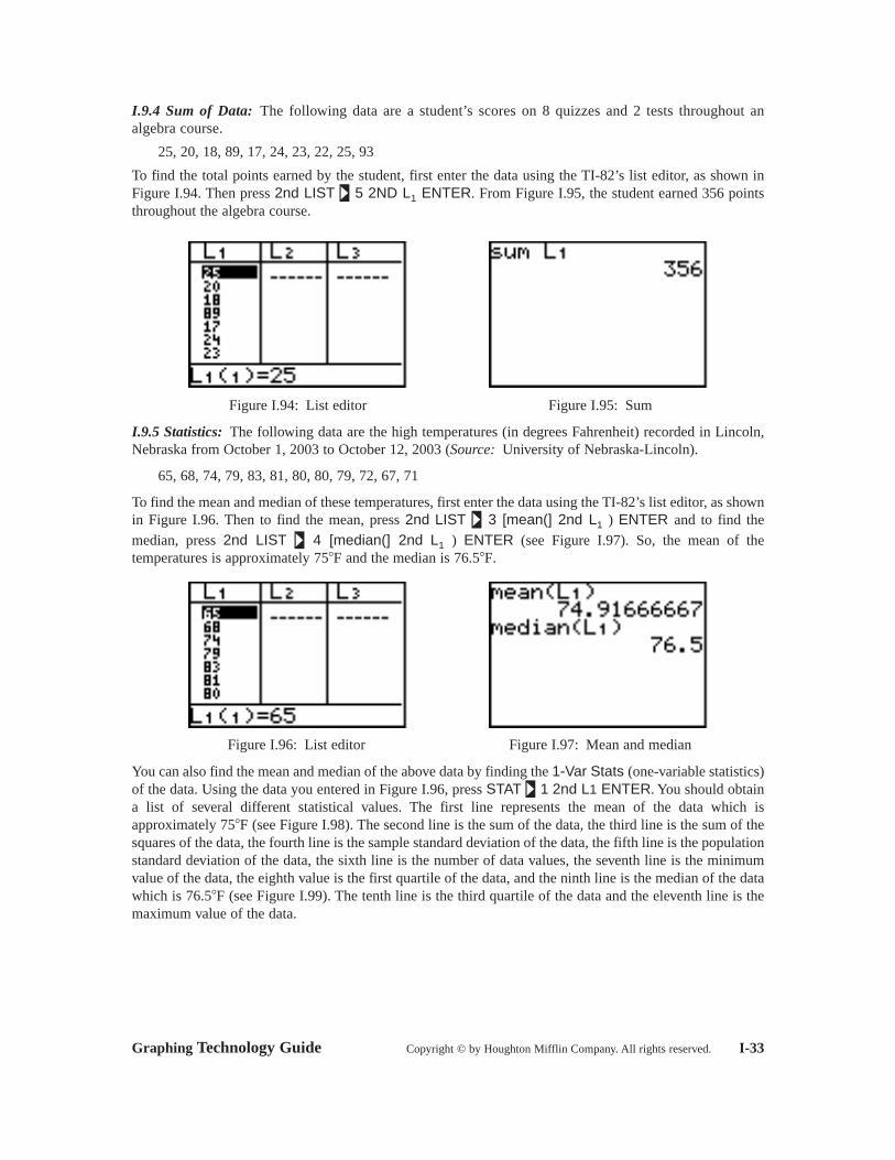
I.9.5 Statistics: The following data are the high temperatures (in degrees Fahrenheit) recorded in Lincoln,Nebraska from October 1, 2003 to October 12, 2003 (Source: University of Nebraska-Lincoln).

65, 68, 74, 79, 83, 81, 80, 80, 79, 72, 67, 71

To find the mean and median of these temperatures, first enter the data using the TI-82’s list editor, as shownin Figure I.96. Then to find the mean, press 2nd LIST 3 [mean(] 2nd ) ENTER and to find the

median, press 2nd LIST 4 [median(] 2nd ) ENTER (see Figure I.97). So, the mean of thetemperatures is approximately and the median is

Figure I.96: List editor Figure I.97: Mean and median

You can also find the mean and median of the above data by finding the 1-Var Stats (one-variable statistics)of the data. Using the data you entered in Figure I.96, press STAT 1 2nd L1 ENTER. You should obtaina list of several different statistical values. The first line represents the mean of the data which isapproximately (see Figure I.98). The second line is the sum of the data, the third line is the sum of thesquares of the data, the fourth line is the sample standard deviation of the data, the fifth line is the populationstandard deviation of the data, the sixth line is the number of data values, the seventh line is the minimumvalue of the data, the eighth value is the first quartile of the data, and the ninth line is the median of the datawhich is (see Figure I.99). The tenth line is the third quartile of the data and the eleventh line is themaximum value of the data.

76.5�F

75�F

76.5�F.75�FL1

L1

L1


Figure I.98: 1-Var Stats Figure I.99: 1-Var Stats

You can scroll through the list of statistical values by pressing or .

I.10 Programming

I.10.1 Entering a Program: The TI-82 is a programmable calculator that can store sequences of commandsfor later replay. Press PRGM to access the programming menu. The TI-82 has space for many programs,each called by a title you give it. The title should be descriptive and can be eight characters, letters, ornumerals long (but the first character must be a letter).

In the program, each line begins with a colon : supplied automatically by the calculator. Any command youcould enter directly in the TI-82’s home screen can be entered as a line in a program. There are also specialprogramming commands.

You may interrupt programming input at any stage by pressing 2nd QUIT. To return later for more editing,press PRGM , move the cursor down to the program’s name, and press ENTER.

You may remove a program from memory by pressing 2nd MEM 2 [Delete…] 6 [Prgm…]. Then move thecursor to the program’s name and press ENTER to delete the entire program.

I.10.2 Executing a Program: To execute a program you entered, press PRGM and then the number or letterit was named. If you have forgotten its name, use the arrow keys to move through the program listing to findits description. Then press ENTER to select the program and enter again to execute it.

If you need to interrupt a program during execution, press ON.

The instruction manual for your TI-82 gives detailed information about programming. Refer to it to learnmore about programming and how to use other features of your calculator.


texas instruments ti-82 graphics calculator i.1 getting - cengage

Documents