Contents lists available at ScienceDirect

Ecological Complexity

journal homepage: www.elsevier.com/locate/ecocom

Original Research Article

Testing the River Continuum Concept with geostatistical stream-networkmodels

Stefano Larsena,b,⁎, Maria Cristina Brunoa, Ian P. Vaughanc, Guido Zolezzia

a Department of Civil, Environmental and Mechanical Engineering, University of Trento, Trento, ItalybDepartment of Sustainable Agro-ecosystems and Bioresources, Research and Innovation Centre, Fondazione Edmund Mach, San Michele all'Adige, Italyc Cardiff School of Biosciences, Cardiff University, Wales, UK

A R T I C L E I N F O

Keywords:Functional feeding groupsMacroinvertebratesLongitudinal gradientSemivariogramsAutocorrelationAdige River

A B S T R A C T

The River Continuum Concept (RCC) provided one of the first unifying frameworks in fluvial ecosystem theory.While the RCC predictions held in many empirical tests, other research highlighted how the model overlookedsources of heterogeneity at different scales e.g. the effects of tributaries. Disentangling these effects requires anassessment of variation in key ecosystem variables over the longitudinal and lateral dimension of river networks.However, so far, no empirical tests have employed a spatially explicit statistical approach to this assessment.

Here, we show how recently-developed spatially-explicit models for river networks can be used to test pre-dictions of the RCC whilst taking into account cross-scale sources of heterogeneity. We used macroinvertebratedata from 195 monitoring sites from 1st to 4th order streams spread across the Adige River network (NE Italy).We compared theoretical expectations with empirical semivariograms that incorporated network topology toassess the continuity and patchiness in the proportion of invertebrates functional feeding groups (FFG) overEuclidean and in-stream distances. Geostatistical stream-network models were then used to quantify the influ-ence of the longitudinal gradient relative to local-scale water quality and land-use drivers, while accounting fornetwork spatial autocorrelation.

Patterns in the semivariograms based on flow-connected relationships were characterised by a nestedstructure associated with heterogeneity at multiple scales. Therefore, the longitudinal variation in FFG wasbetter described by a patchy discontinuum rather than a gradient, implying that both in-stream processes andlandscape factors influenced stream ecosystem function. The overall shift in FFG along the longitudinal profilewas generally consistent with the RCC predictions, although the best models often included water quality andlocal land-use predictors. Stream-network models further indicated that up to 90% of residual variation(mean=50%) was accounted for by spatial autocorrelation, especially among flow-connected communities.Accounting for such autocorrelation not only improved model performance relative to non-spatial approaches,but indicated that most flow-connected communities were spatially correlated to some extent. This has clearimplications for the assessment of the RCC tenets. This is the first test of the river continuum model that ex-plicitly accounted for stream network topology and autocorrelation. Results indicated that in the Adige River,macroinvertebrates feeding groups exhibited heterogeneity along the longitudinal gradient, which appearedpunctuated by local habitat transitions. Such transitions could be associated with artificial impoundments thatalter the natural continuity of river processes, and we advocate the use of spatially explicit network models totest the RCC in more natural contexts.

1. Introduction

The distribution and diversity of aquatic organisms in river net-works is predominantly influenced by the downstream direction ofwater flow and by the physical changes occurring along the long-itudinal gradient (Townsend, 1996; Ward, 1989). This concept is at the

heart of early conceptual models aimed at idealizing the structure andfunction of communities along river systems such as the river zonation(Hawkes, 1975; Illies, 1961) and the River Continuum concepts(Vannote et al., 1980). In particular, the River Continuum Concept(RCC) provides a useful conceptualisation of river networks as openecosystems characterised by a continuum of physical changes and

https://doi.org/10.1016/j.ecocom.2019.100773Received 18 March 2019; Received in revised form 21 May 2019; Accepted 20 July 2019

⁎ Corresponding author at: Department of Civil, Environmental and Mechanical Engineering, University of Trento, Trento, Italy.E-mail addresses: stefano.larsen@fmach.it, larsen.stefano@gmail.com (S. Larsen).

Ecological Complexity 39 (2019) 100773

1476-945X/ © 2019 Elsevier B.V. All rights reserved.

T

associated ecological responses, in which the type and availability oforganic matter, the structure of invertebrate communities and thepartitioning of resources shift gradually along the longitudinal gradient.Although the RCC is a simplification that overlooks the patchy nature ofriver systems associated with local geology, tributary effects and lateralfloodplain inputs (e.g. Thorp et al., 2006), it remains one of the mostinfluential concepts in river science (4.949 citations as of Match 2019;ISI Web of Science database). One of the key strengths of the RCC is thatit proposes testable hypotheses regarding changes in stream metabolism(P/R), the main trophic basis of production (carbon sources) and theconsequent adjustment of consumer communities (functional feedinggroups; Cummins, 2016)

Empirical tests of the RCC provided support for its predictions,especially in temperate North American rivers (Curtis et al., 2018;Hawkins and Sedell, 1981; Minshall et al., 1985, 1983; Rosi-Marshalland Wallace, 2002; Webster, 2007), and more recently in differentbiomes and climatic zones (Greathouse and Pringle, 2006; Jiang et al.,2011; Tomanova et al., 2007). Studies that have criticised the RCCgenerally emphasise the local heterogeneity of river systems (Perry andSchaeffer, 1987; Statzner and Higler, 1985; Townsend, 1989). For in-stance, Pool (2002) argued that local factors such as reach geomor-phology or bedrock geology could override longitudinal gradients, sothat stream communities in a given segment may be just as similar tocommunities far up or downstream as they are to those in neighbouringstretches. The issue of quantifying the relative contributions of ‘global’river gradients and local heterogeneity is currently acknowledged (e.g.Thorp, 2014), and may in part stem from the methodological challengesof describing patterns and testing alternative hypotheses in dendriticnetworks. Standard statistical methods are unable to handle the com-plexities resulting from linear river reaches arranged into complexbranching networks and the influence of directional water movement(Peterson et al., 2013). Spatial autocorrelations are, in fact, particularlycomplex in river systems as their intensity varies with the connectivityand directionality within the network (Isaak et al., 2014). In this case,models based on Euclidean distances, for instance, might be insufficient

to represent the unique spatial relationships found in river systems(Peterson et al., 2013). These considerations are particularly relevantfor the RCC where one fundamental aspect of the continuum is thatecological processes in downstream reaches are linked to those occur-ring upstream (e.g. Minshall et al., 1985). Moreover, critics to thecontinuum model emphasised how river systems display heterogeneityat multiple spatial scales besides the longitudinal dimension (Perry andSchaeffer, 1987; Poole, 2002). It is therefore surprising that none of theprevious empirical tests of the RCC model employed any spatially ex-plicit approach that could either account for autocorrelation or utilisethe spatial variance as part of the study.

Fortunately, recent advances in the field of geospatial statisticsadapted to dendritic networks provide the tools to quantify the mainscales of spatial variation within river networks and allow for morerigorous tests of hypotheses such as the RCC (Peterson and Hoef, 2010;Ver Hoef and Peterson, 2010). Two developments in particular arevaluable for assessing RCC. The first is the generalisation of the stan-dard geostatistical tool, the semivariogram, to river networks (calledTorgegrams; Peterson et al., 2013). Variograms quantify spatial struc-ture and can reveal the dominant scales of environmental processes(Cressie, 1993). Specifically, semivariograms depict the autocorrelationof a given variable calculating the semivariance between pairs of ob-servations for a range of watercourse distance lags (h) as:

∑= − +=

γ hN h

z s z s h( ) 12 ( )

[ ( ) ( )]i

N

i i1

2

where N(h) is the number of observation pairs separated by distance lagh, z(si) is the value of the variable in location si, and z(si+h) is the valueat distance h from si.

The shapes of the semivariograms can be compared with theoreticalexpectations reflecting hypothesised spatial structures and dependency(Fig. 1).

In river networks, semivariograms can be calculated based on threespatial distances among sampling locations: flow-connected (water-course distance between locations connected by water flow), flow-

Fig. 1. Hypothetical distribution of avariable mapped along a river network(e.g. proportion of one feeding groupin the community) and the associatedsemivariograms. In A), there is nospatial structure in the variance at thesampled scale. The intercept of thesemivariance function (called‘nugget’) represents the variance dueto sampling error or variation at scalesfiner than the shortest separation dis-tance. In B), spatial dependency atlarge-scale reflects a single dominantgradient of variation from upstream todownstream. The values where thesemivariance function reaches a pla-teau (called ‘range’), indicates thedistance at which values are con-sidered independent from each other.In C), small-scale heterogeneity re-flects patchiness and discontinuitywhere, for instance, factors influen-cing the variable operate at fine scales,and the range is reached at shorterdistances. In D), nested heterogeneityreflects a combination of small-scalepatchiness embedded in a larger-scalegradient (with multiple inflectionpoints). In this case, patterns are in-fluenced by factors operating at mul-tiple scales. Figure is re-drawn afterMcGuire et al. (2014).

S. Larsen, et al. Ecological Complexity 39 (2019) 100773

2

unconnected (watercourse distance between any locations in the net-work) and Euclidean. Specifically, semivariograms of flow-connectedrelationship describe the effects of hydrologic transport and upstreamdependence and can thus indicate whether the longitudinal gradientrepresents the dominant scale of variability in the distribution of carbonsources and consumers (a key tenet of the RCC). Conversely, patternsfrom the semivariograms based on flow-unconnected and Euclideanrelationships can inform on the influence of adjacent tributaries andwider landscape properties independent of network position, respec-tively (McGuire et al. 2014). Thus, when used deductively, empiricalspatial patterns can help formulate hypotheses regarding the mainprocesses influencing the distribution of the variables of interest(McIntire and Fajardo, 2009).

The second major development is stream-network models that ex-tend conventional linear models to account for the branching structureof the network and the directionality of water flow, as well as the 2-Dterrestrial matrix in which the network is embedded. Therefore, theycan simultaneously account for both along-channel and across catch-ment (Euclidean) patterns of autocorrelation (Ver Hoef andPeterson, 2010). Notably, equivalent models that assume differenttypes of spatial correlation (e.g. flow-connected, flow-unconnected andEuclidean, the latter ignoring the network structure) can be comparedto assess alternative hypotheses regarding spatial dependency.

In this study, we first used semivariograms based on Euclidean andstream-network distances (Torgegrams) to visualise patterns and scalesof variability in the distribution of macroinvertebrate functionalfeeding groups (FFG) along the longitudinal river gradients (consistentwith RCC), and across the whole catchment in a large Alpine rivernetwork. We focussed on invertebrate FFG because their variation overthe continuum represents a central prediction of the RCC, linking basalcarbon sources to consumer communities. Moreover, macroinvertebratedata are routinely collected for bio-monitoring purposes and theirfeeding habits are well known (Schmidt-Kloiber and Hering, 2015).Subsequently, we used geostatistical stream-network models to quan-tify the importance of the longitudinal gradient relative to local scalehabitat variables, while accounting for spatial autocorrelation withinthe network. Whilst previous studies have considered the shift of in-vertebrate FFG along the river gradient (Greathouse and Pringle, 2006;Grubaugh et al., 1996; Jiang et al., 2011; Minshall et al., 1985), this isthe first time a geostatistical approach has been employed that speci-fically accounts for spatial autocorrelation in dendritic networks.

The RCC was originally based on forested temperate high-reliefbasins in North America. While the Adige River conforms to these as-pects, its longitudinal continuity is altered by numerous hydropowerdams distributed over the basin (Chiogna et al., 2016a; Larsen et al.,2019), which are expected to alter the natural continuity of river pro-cesses (Hoenighaus et al., 2007; Humphries et al., 2014). Therefore, thepresent study should not be considered as a formal test of the validity ofthe RCC model. Rather, we propose a statistically robust approach totest its predictions to a case study that well represents many Alpineriver catchments across Europe and North America.

2. Study area and dataset

The Adige River (Fig. 2) is the third largest river basin in Italy,covering more than 12,000 km2. Most of the Adige River drains theAlpine region with elevation reaching 3400m a.s.l. Climate is typicallyAlpine with dry winters, snow and glacier melt in spring and ratherhumid summers and autumns (Lutz et al., 2016). Since the beginning oflast century, more than 30 dams have been built across the wholenetwork (i.e. dams are distributed over 1st to 4th order streams), mostlyfor hydropower generation. These dams have altered the natural flowregimes of many reaches (Larsen et al., 2019; Zolezzi et al., 2009), andlikely disrupted the natural continuum of sediment and organic mattertransport.

Macroinvertebrate data were collected as part of the institutional

monitoring programmes of the Environmental Protection Agencies ofthe Provinces of Trento and Bolzano. Sampling occurred between 2009and 2014 in 195 reaches from 1st to 4th order streams (between 130 and1980m a.s.l.). Sites were sampled multiple times in different seasons. Inany given year, between 91 and 161 sites (median=113) were in-cluded. The number of samples per site ranged between 2 and 12 (mean= 4.8), but most sites (80%) were sampled 3–9 times, mostly in springand autumns. Macroinvertebrate densities were averaged to representthe typical community composition of a reach and remove seasonaleffects. Sampling followed the multi-habitat approach where 10-re-plicate Surber samples were distributed over a 20–50m reach in pro-portion to the different microhabitat types present (Hering et al., 2004).Macroinvertebrates were identified to genus and family level(Appendix A).

3. Methods

3.1. Ecological trait and local environmental data

Information about invertebrate feeding traits was gathered from theonline database on the ecology of freshwater organisms (www.freshwaterecology.info; Schmidt-Kloiber and Hering, 2015). To testthe RCC predictions, we considered the following feeding groups: gra-zers, shredders, gatherers, filterers and predators. A fuzzy approach wasused to assign each taxon an affinity score for each feeding group, thusavoiding restricting taxa to a specific feeding group and effectivelytaking into account intra-specific variability (Chevenet et al., 1994).Affinities at family and genus levels were obtained by averaging scoresover the species known to occur in the region. Affinity scores were thenstandardised between 0 and 1 and then weighted by each taxon's re-lative abundance (using the ‘functcomp’ command within the FDpackage in R) to calculate the community-wide proportion of FFG foreach site (Schmera et al., 2014).

To quantify the position along the longitudinal river continuum foreach of the 195 study reaches, a synthetic variable was created usingprincipal component analysis (PCA) of Strahler stream order, distancefrom ‘mouth’ (i.e. most downstream reach), altitude and upstreamcatchment area. The first principal component (‘Longitudinal PC1’)explained c. 60% of the variation and was negatively correlated withdistance from ‘mouth’ and altitude, and positively correlated withStrahler order and catchment area (Table 1). This PC reflected thelongitudinal position and allowed us to score each sample location overthe network according to a continuous longitudinal gradient that ac-counted for multiple aspects (Jiang et al., 2011; Tomanova et al., 2007;Vaughan et al., 2013).

ArcMap 10.5 and the STARS toolset (Peterson and Hoef, 2014) wereused to calculate distance matrices (flow-connected, flow-unconnectedand Euclidean), upstream catchment areas and the spatial weightsneeded in the network-models (see below). Shapefiles of the rivernetwork and catchment topography were obtained by the Environ-mental Protection Agencies of the Provinces of Trento and Bolzano.

Three reach-scale environmental variables were also included in theanalyses. The first two were the proportions of agricultural and forestland cover within a 1-km buffer around each sampling location asproxies for allochthonous input and shading, i.e., among the maincontributing factors to the longitudinal gradients in the RCC. The thirdvariable was the stream water physico-chemical status, expressed bythe WFD (Water Framework Directive, EU 2000/60) LIMeco index(Livello di Inquinamento dai Macrodescrittori per lo stato ecologico),which is the official water-quality indicator in Italy. This is a multi-metric index that scores water quality based on threshold levels fordissolved oxygen, ammonia and nitrate concentrations and total phos-phorus (see Azzellino et al., 2015).

S. Larsen, et al. Ecological Complexity 39 (2019) 100773

3

3.2. Semivariograms

Empirical variograms and Torgegrams were compared with theo-retical expectations (Fig. 1) and used to examine the dominant spatialscale of variation in the proportion of feeding groups along and acrossthe river network. For instance, a continuous single scale of variation inthe proportion of a feeding group along the river continuum wouldproduce variograms like those in Fig. 1B. Conversely, a completedominance of local-scale drivers would produce variograms likeFig. 1C, while a patchy continuum would generate variograms such asFig. 1D. Using Euclidean and in-stream distances, the continuity andpatchiness of the spatial patterns can be separately examined over the2D and longitudinal dimensions of river networks.

Torgegrams were also used as preliminary exploratory analysis tovisually examine the patterns in semivariance between flow-connectedand flow-unconnected site pairs in order to guide the selection of au-tocovariance function in the subsequent stream-network modelling(Ver Hoef et al., 2014).

3.3. Stream network models

In a subsequent analysis, we used stream-network models (Ver Hoefet al., 2014; Ver Hoef and Peterson, 2010) to quantify the importance ofthe longitudinal continuum (expressed as the Longitudinal PC1) re-lative to local-scale environmental factors (i.e. water quality and land-use) as predictors of FFG proportions. All the spatial data necessary toanalyse stream-network models were generated in ArcMap 10.5 usingthe STARS toolset. We accounted for the complex autocorrelationstructure of dendritic networks using Euclidean as well as in-streamflow-connected and flow-unconnected autocovariance functions.

Stream-network models are variance components models that takethe general form:

= + + + +y Xβ z z z εTU TD E

where y is the response variable vector (here: logit transformed pro-portion of feeding groups), X is the matrix of covariates (here: long-itudinal PC1, LIMeco, land-use), zTU+zTD+zE are vectors of zero-meanrandom variables with autocorrelation structure based on tail-up, tail-down and Euclidean functions, and ɛ is the vector of random in-dependent errors. The tail-up and tail-down autocovariance structuresare moving-average functions that quantify autocorrelation amongflow-connected and flow-unconnected locations, respectively (Isaaket al., 2014; Peterson et al., 2013). The autocovariance functions cantake different forms, including linear-with-sill, spherical, Mariah andexponential models (Garreta et al., 2009), but spatial models are gen-erally robust against their mis-specification (Garreta et al., 2009; Isaaket al., 2014). Specifically, the tail-up function permits correlation

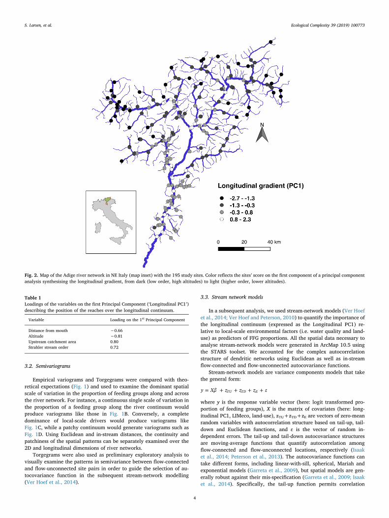
Fig. 2. Map of the Adige river network in NE Italy (map inset) with the 195 study sites. Color reflects the sites’ score on the first component of a principal componentanalysis synthesising the longitudinal gradient, from dark (low order, high altitudes) to light (higher order, lower altitudes).

Table 1Loadings of the variables on the first Principal Component (‘Longitudinal PC1’)describing the position of the reaches over the longitudinal continuum.

Variable Loading on the 1st Principal Component

Distance from mouth −0.66Altitude −0.81Upstream catchment area 0.80Strahler stream order 0.72

S. Larsen, et al. Ecological Complexity 39 (2019) 100773

4

exclusively between sites that are flow-connected (sites not connectedare assumed independent) and uses a weighting approach to up- anddown-weight samples that occur upstream of a given location. Here, weused upstream catchment area as surrogate of discharge for theweighting procedure. In this case, the moving-average autocorrelationfunction is split at confluences so that locations on larger streams have astronger influence on downstream communities than locations insmaller streams (Peterson et al., 2013). The tail-down function allowscorrelation among both flow-connected and unconnected samples andtherefore a spatial weighting measure is not necessary (Isaak et al.,2014). Finally, the Euclidean functions is based on Euclidean distancesas in the traditional spatial statistics methods. Therefore, stream-net-work models are flexible tools that can incorporate multiple informa-tion into a single model (Ver Hoef and Peterson, 2010). Moreover, byallowing errors to be differently autocorrelated over the longitudinaland lateral network dimension they can indirectly account for the ef-fects of unmeasured variables that have a spatial pattern (e.g. soil,underlying bedrock geology).

The values of FFG in the communities were logit-transformed asrecommended for proportional data (Warton and Hui, 2011) andparameter estimation was based on maximum-likelihood. Covariateselection was then based on Akaike Information Criterion (AIC;Burnham and Anderson, 2002), but to describe overall model perfor-mance we also report root-mean-square prediction errors (RMSPE),which specifically focus on model predictive power. Overall modeldevelopment was a step-wise process. We first included all predictors(i.e. longitudinal PC1, LIMeco, and local land-use) and the full mixtureof autocovariance functions, which included an exponential tail-up,tail-down and Euclidean models (Ver Hoef et al., 2014). Then we used amanual step-wise approach to remove non-significant predictors fromthe model. We then refined the spatial component comparing (or re-moving) different functions for the tail-up, tail-down and Euclideanautocovariance structure to select the final model with the lowest AIC.The spatial components were investigated after the selection of cov-ariates since the model accounts for spatial autocorrelation in the errorsafter the effects of the covariates have been removed. Therefore, pat-terns of spatial dependency are data and model specific and can changeif the covariates change (e.g. Frieden et al., 2014). The efficacy of theselected spatial model relative to a non-spatial model (ignoring anyspatial autocorrelation) was also evaluated (Isaak et al., 2014). Spatialstream-network models were run in R (R Core Team, 2017) using theSSN package (Ver Hoef et al., 2014). For each site, raw data about FFGproportions, taxon richness, Longitudinal PC1, and geographic co-ordinates are given as Supplementary Material.

4. Results

4.1. Empirical semivariograms

The semivariograms for Euclidean and flow-unconnected relation-ships (Fig. 3) were consistent with the presence of a single dominantspatial structure, with variance progressively increasing with distancefor all FFGs. These patterns resemble Fig. 1B and suggest the presenceof a catchment-wide gradient. Conversely, when accounting for flow-connections (limiting the modelled spatial autocorrelation to occur onlyamong sites connected by water flow), nested spatial structuresemerged that are associated with heterogeneity at multiple scales (i.e.multiple inflection points at different distances, resembling Fig. 1D).The flow-connected semivariogram is the most relevant to the RCC, andshows that the spatial distribution of FFG does not vary as a continuumalong the longitudinal gradient, but is highly heterogeneous.

The semivariogram for taxonomic richness was mostly indicative ofa single scale of variation, especially across the lateral dimension of thestream network (Euclidean and flow-unconnected relationships).Patterns from the flow-connected relationships exhibited some hetero-geneity, which was less marked than that characterising FFG, and with

an inflection point evident at larger distances.

4.2. Stream-network models

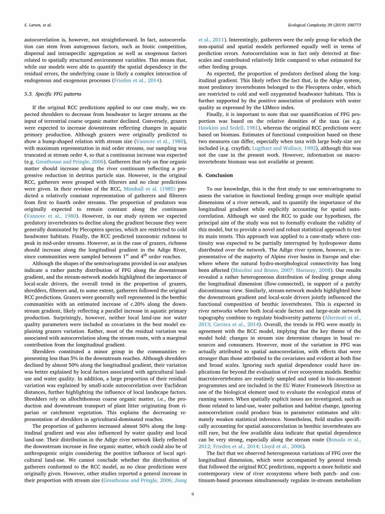
Stream network models were in broad agreement with the RCCpredictions (Table 2; Fig. 4), with an increase in grazers and gatherersalong the longitudinal gradient, and a decrease in the shredders. Fil-terers were not related to the longitudinal gradient while, contrary tothe original RCC predictions, predators declined. Taxon richness wasunrelated to the longitudinal profile. However, the relative importanceof local-scale drivers and the influence of spatial autocorrelation dif-fered substantially among FFG (Table 2).

4.3. Grazers

Grazers were primarily represented by Ephemeroptera (Baetis,Ecdyonurus) and Chironomidae.

Longitudinal PC1 explained 8% of the variance in the proportion ofgrazers in the non-spatial model (i.e. ignoring any spatial autocorrela-tion), which declined to 5% when autocorrelation was accounted for.There was no evidence for an effect of land-use or water quality para-meters.

Overall, the model with the lowest AIC and RMSPE was the spatialmodel with a tail-up and Euclidean autocovariance functions. Most ofthe residual variation (77%) was captured by the tail-up autocovariancefunction at a relatively large scale (estimated range of c.60 km). Thisindicates that grazer communities in flow-connected sites exhibitedspatial autocorrelation that accounted for most of their variation alongthe network.

4.4. Shredders

The proportion of shredders (mostly represented by Limnephilidae,Leuctra and Gammaridae) declined along the longitudinal gradient,which alone explained 17% of their variation in the non-spatial modeland about 16% in the spatial-model.

However, according to the AIC, the best models describing shred-ders variation did not include the longitudinal gradient, but only theLIMeco index and the proportion of agricultural land-use for 1-kmbuffer around the site. The non-spatial and the spatial models wereequally supported according to the AIC (delta AIC = 0.2), although thespatial model had smaller prediction errors. In the spatial model, mostof the residual variation was accounted for by a small-scale Euclideanautocovariance function (estimated range=1.5 km).

These results indicated that, overall, the variation in the proportionof shredders over the network was mostly influenced by local scalefactors rather than by the longitudinal gradient.

4.5. Gatherers

The proportion of gatherers (represented by Ephemeroptera andPlecoptera such as Serratella and Amphinemura among others) increasedalong the longitudinal river gradient, which alone explained 19 and18% of their variance in the non-spatial and spatial model, respectively.

According to the AIC, the most supported model was the non-spatialmodel that included the longitudinal gradient as well as the LIMeco andthe agricultural land-use. The best spatial model required only a small-scale tail-up function (estimated range= 8 km), which accounted forabout 17% of the residual variation. Overall, the proportion of gath-erers appeared determined by both local scale factors and the long-itudinal position along the network with relatively fine-scale auto-correlation among flow-connected communities.

4.6. Filterers

Filterers (mostly Hydropsychidae and Simuliidae) did not show any

S. Larsen, et al. Ecological Complexity 39 (2019) 100773

5

significant relationship with the longitudinal gradient in either non-spatial or spatial models. The most supported model was a spatialmodel with only the LIMeco index as covariate and a tail-down (re-presenting flow-unconnected relationships) and Euclidean auto-covariance functions, which accounted for a similar proportion of re-sidual variation. The best non-spatial model included the LIMeco indexand the proportion of woodland in 1-km buffer. Both models howevershowed high residual errors (∼1) indicating that the proportion of filterfeeders was influenced by other factors besides the one considered here.Contrary to what observed in other feeding groups, autocorrelationamong flow-connected filterer communities was not included in thebest spatial models. Rather, autocorrelation occurred mostly across thelateral dimension of the network as modelled by the tail-down andEuclidean functions (relationship between locations not upstream-downstream of each other).

4.7. Predators

Predators primarily included Plecoptera (Isoperla, Perlodes) andTrichoptera Rhyacophilidae.

In contrast to the RCC prediction, the proportion of predators de-clined along the longitudinal gradient, which alone explained 29 and27% of variation in the non-spatial and spatial model respectively. Thenon-spatial model was the most supported and included the long-itudinal gradient and the LIMeco index as covariates, jointly accountingfor 41% of predators’ variation. The spatial model had, however, thelowest prediction errors and included the same covariates with a large-scale tail-up (range= 100 km) and Euclidean autocovariance functions

that accounted for 40% of residual variation.

4.8. Taxon richness

Taxonomic richness was not related to the longitudinal river gra-dient. The best non-spatial and spatial models selected partially dif-ferent covariates. The most supported model included a tail-up andEuclidean autocovariance functions that jointly explained c.40% of theresidual variation, while the selected covariates only explained 8%. Theestimated range for the flow-connected autocovariance model wasmuch longer than the total length of the river network (1000 km), in-dicating that measurements of invertebrate richness in all flow-con-nected communities were correlated to some extent.

5. Discussion

The River Continuum Concept is one of the most influential theo-retical frameworks in river ecology, idealising river network as openecosystems in which the physical template and the associated ecologicalprocesses change predictably along the longitudinal continuum. TheRCC immediately stirred a lively debate that stimulated empirical testsas well as conceptual revisions (e.g. Minshall et al., 1985; Statzner andHigler, 1985). Critics to the RCC argued that the model overlooked theimportance of lateral floodplain inputs, tributary effects, and fine-scaleheterogeneity, as well as human impacts (Perry and Schaeffer, 1987;Poole, 2002). As such, ecological processes and functions along theriver network were better described by punctuated discontinuity ratherthan by a continuum.

Fig. 3. Empirical semivariograms of the proportion of feeding traits and taxon richness based on Euclidean, flow-connected and flow-unconnected distances. Note thechange in the y-axis. The number of observation pairs from which semivariances are calculated differs among distance lags, with fewer pairs contributing to measuresat larger distances. The semivariance values are expressed as x1000, except for taxon richness.

S. Larsen, et al. Ecological Complexity 39 (2019) 100773

6

Testing the key tenets of the RCC and its caveats rely upon detectingspatial patterns and discriminating between patterns generated by dif-ferent processes. So far, however, empirical tests of the RCC - eithersupporting or confuting its predictions – have not used spatially explicitstatistical approaches. Ignoring spatial autocorrelation (i.e. non-in-dependence) among field measurements can produce bias in parameterestimates and increase the chance of Type I errors (Legendre, 1993). Inaddition, patterns of spatial autocorrelation, which are often perceivedas data nuisance, can instead be used to appraise the dominant scale ofvariation in a given variable (Dray et al., 2012). This has clear im-plications for the assessment of the RCC model, or any spatial patternsin river networks.

Here we combined the analyses of semivariograms with geostatis-tical stream-network models, to (i) assess the continuity and hetero-geneity in the proportion of invertebrate feeding groups over the

longitudinal and lateral dimensions of the network and (ii) quantify therelative importance of the longitudinal gradient vs. local drivers, whilespecifically accounting for the spatial autocorrelation inherent to den-dritic networks.

5.1. Semivariograms

The semivariograms indicated that in the Adige river network var-iation in feeding groups along the longitudinal continuum (flow-con-nected relationships) was characterised by nested spatial structureswith multiple inflection points. This supports the hypothesis thatdownstream variation in carbon sources and associated consumers werebetter represented by a patchy discontinuum rather than by a gradient(Rice et al., 2001). This implies that both in-stream factors and local-scale drivers influenced invertebrates’ structure and function along the

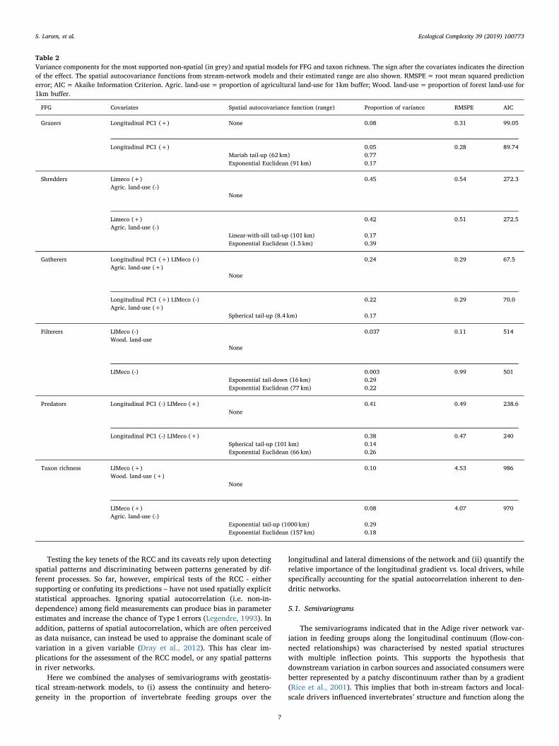
Table 2Variance components for the most supported non-spatial (in grey) and spatial models for FFG and taxon richness. The sign after the covariates indicates the directionof the effect. The spatial autocovariance functions from stream-network models and their estimated range are also shown. RMSPE= root mean squared predictionerror; AIC=Akaike Information Criterion. Agric. land-use= proportion of agricultural land-use for 1km buffer; Wood. land-use=proportion of forest land-use for1km buffer.

FFG Covariates Spatial autocovariance function (range) Proportion of variance RMSPE AIC

Grazers Longitudinal PC1 (+) None 0.08 0.31 99.05

Longitudinal PC1 (+) 0.05 0.28 89.74Mariah tail-up (62 km) 0.77Exponential Euclidean (91 km) 0.17

Shredders Limeco (+) 0.45 0.54 272.3Agric. land-use (-)

None

Limeco (+) 0.42 0.51 272.5Agric. land-use (-)

Linear-with-sill tail-up (101 km) 0.17Exponential Euclidean (1.5 km) 0.39

Gatherers Longitudinal PC1 (+) LIMeco (-) 0.24 0.29 67.5Agric. land-use (+)

None

Longitudinal PC1 (+) LIMeco (-) 0.22 0.29 70.0Agric. land-use (+)

Spherical tail-up (8.4 km) 0.17

Filterers LIMeco (-) 0.037 0.11 514Wood. land-use

None

LIMeco (-) 0.003 0.99 501Exponential tail-down (16 km) 0.29Exponential Euclidean (77 km) 0.22

Predators Longitudinal PC1 (-) LIMeco (+) 0.41 0.49 238.6None

Longitudinal PC1 (-) LIMeco (+) 0.38 0.47 240Spherical tail-up (101 km) 0.14Exponential Euclidean (66 km) 0.26

Taxon richness LIMeco (+) 0.10 4.53 986Wood. land-use (+)

None

LIMeco (+) 0.08 4.07 970Agric. land-use (-)

Exponential tail-up (1000 km) 0.29Exponential Euclidean (157 km) 0.18

S. Larsen, et al. Ecological Complexity 39 (2019) 100773

7

longitudinal gradient. Part of the observed discontinuity in FFG varia-tion along the Adige River is likely associated with the presence ofartificial impoundments. Hydropower dams are expected to alter therelative availability of different carbon sources in complex ways, bychanging not only flow patterns, but also temperature regime and waterchemistry (Zolezzi et al., 2011, 2009). For instance, consumers inreaches below dams often derive their carbon sources from local pro-duction and riparian input rather than upstream transport, thuscreating a gap in the downstream transition (Hoenighaus et al., 2007;Poole, 2002). Assessing this, however, would require more detailedlocal-scale sampling up- and downstream of impoundments.

Conversely, patterns of variation over the whole catchment, ig-noring the effects of flow direction, (flow-unconnected and Euclideanrelationships), were consistent with the presence of large-scale spatialstructure, with little or no fine-scale heterogeneity (cf. Fig. 1B). Thesesemivariograms describe relationships among communities associatedwith wider landscape properties (e.g. gradient in underlying catchmentgeology; Chiogna et al., 2016b) and showed that similarity in the pro-portion of feeding groups generally decreased with spatial separation.

The shape of the semivariograms for taxonomic richness indicated arather homogeneous distribution, especially over Euclidean and flow-unconnected distances and with large estimated ranges. Indeed, whilecomposition is expected to differ with increasing spatial separation(Soininen et al., 2007), the richness of communities can be similar overlarge distances and across a range of conditions (Bonada et al., 2012;Larsen et al., 2018). Moreover, the variance from flow-connected re-lationships was always lower than that based on lateral relationships,indicating that connected communities were generally more similar toeach other in terms of taxon richness.

It is important to note, however, that the shape of the variograms isinfluenced by the overall sampling design and especially by theminimum and maximum distance between samples as well as the dis-persal capacity of the organisms involved (Ettema and Wardle, 2002).Therefore, variograms across different studies and/or organisms shouldbe compared with caution.

5.2. Stream-network models

When significant, the effect of longitudinal gradient explained be-tween 5% and 29% of variation. However, the best models did not al-ways include the longitudinal gradient as covariate, as in the case ofshredders and taxon richness. It is well known that many factors acrossa range of scales influence macroinvertebrate richness and function(e.g. Karaus et al., 2013; Richards et al., 1997), with effect that can beindependent from the longitudinal dimension. This was evident here inthe inclusion of local land-use and water quality in most of the sup-ported models. Moreover, stream-network models indicated that FFGexhibited predictable spatial patterns that could not be accounted for bylocal variables with substantial autocorrelation especially among flow-connected communities. Taken together the autocovariance functionsexplained between 17% and 94% of residual variation with a mean of50%. That is, half of the variation in the proportion of feeding groupswas, on average, accounted for by spatial autocorrelation either alongthe stream route or across the network. Accounting for this auto-correlation always improved model performance as measured by theprediction errors (RMSE), as often observed in other studies usingstream-network models (Isaak et al., 2014).

Autocorrelation among flow-connected locations is the most re-levant to the RCC because it represents the relationship along thedownstream continuum. Tail-up functions alone explained between14% and 77% of variation, with an estimated range that varied greatly,from 6 km, to 100 km and up to 1000 km in the case of taxon richness.This means that most flow-connected communities exhibited some de-gree of spatial correlation. Therefore, the most relevant continuum inthe Adige river system appears to be the spatial correlation that existsamong flow-connected locations.

The importance of spatial autocorrelation over the lateral dimensionwas well captured by the Euclidean autocovariance function. This ex-plained up to 39% of variation in feeding groups with effects estimatedat both fine (1.6 km range) and large-scale (150 km range). This againindicates that landscape features and local drivers other than the po-sition along the continuum contributed to the observed variation infeeding groups.

Understanding the processes underpinning the observed

Fig. 4. Plot of the proportion of feedingtraits and taxonomic richness along theriver longitudinal dimension as ex-pressed by the first PC (Adige rivernetwork; 195 reaches). A linear re-gression line is shown when the re-lationship was significant. Note: theregression lines are corrected for spa-tial autocorrelation employing the fullmixture of autocovariance functions.

S. Larsen, et al. Ecological Complexity 39 (2019) 100773

8

autocorrelation is, however, not straightforward. In fact, autocorrela-tion can stem from autogenous factors, such as biotic competition,dispersal and intraspecific aggregation as well as exogenous factorsrelated to spatially structured environment variables. This means that,while our models were able to quantify the spatial dependency in theresidual errors, the underlying cause is likely a complex interaction ofendogenous and exogenous processes (Frieden et al., 2014).

5.3. Specific FFG patterns

If the original RCC predictions applied to our case study, we ex-pected shredders to decrease from headwater to larger streams as theinput of terrestrial coarse organic matter declined. Conversely, grazerswere expected to increase downstream reflecting changes in aquaticprimary production. Although grazers were originally predicted toshow a hump-shaped relation with stream size (Vannote et al., 1980),with maximum representation in mid order streams, our sampling wastruncated at stream order 4, so that a continuous increase was expected(e.g. Greathouse and Pringle, 2006). Gatherers that rely on fine organicmatter should increase along the river continuum reflecting a pro-gressive reduction in detritus particle size. However, in the originalRCC, gatherers were grouped with filterers and no clear predictionswere given. In their revision of the RCC, Minshall et al. (1985) pre-dicted a relatively constant representation of gatherers and filterersfrom first to fourth order streams. The proportion of predators wasoriginally expected to remain constant along the continuum(Vannote et al., 1980). However, in our study system we expectedpredatory invertebrates to decline along the gradient because they weregenerally dominated by Plecoptera species, which are restricted to coldheadwater habitats. Finally, the RCC predicted taxonomic richness topeak in mid-order streams. However, as in the case of grazers, richnessshould increase along the longitudinal gradient in the Adige River,since communities were sampled between 1st and 4th order reaches.

Although the shapes of the semivariograms provided in our analysesindicate a rather patchy distribution of FFG along the downstreamgradient, and the stream-network models highlighted the importance oflocal-scale drivers, the overall trend in the proportion of grazers,shredders, filterers and, to some extent, gatherers followed the originalRCC predictions. Grazers were generally well represented in the benthiccommunities with an estimated increase of c.20% along the down-stream gradient, likely reflecting a parallel increase in aquatic primaryproduction. Surprisingly, however, neither local land-use nor waterquality parameters were included as covariates in the best model ex-plaining grazers variation. Rather, most of the residual variation wasassociated with autocorrelation along the stream route, with a marginalcontribution from the longitudinal gradient.

Shredders constituted a minor group in the communities re-presenting less than 5% in the downstream reaches. Although shreddersdeclined by almost 50% along the longitudinal gradient, their variationwas better explained by local factors associated with agricultural land-use and water quality. In addition, a large proportion of their residualvariation was explained by small-scale autocorrelation over Euclideandistances, further highlighting the influence of local landscape factors.Shredders rely on allochthonous coarse organic matter, i.e., the pro-duction and downstream transport of plant litter originating from ri-parian or catchment vegetation. This explains the decreasing re-presentation of shredders in agricultural-dominated reaches.

The proportion of gatherers increased almost 50% along the long-itudinal gradient and was also influenced by water quality and localland-use. Their distribution in the Adige river network likely reflectedthe downstream increase in fine organic matter, which could also be ofanthropogenic origin considering the positive influence of local agri-cultural land-use. We cannot conclude whether the distribution ofgatherers conformed to the RCC model, as no clear predictions wereoriginally given. However, other studies reported a general increase intheir proportion with stream size (Greathouse and Pringle, 2006; Jiang

et al., 2011). Interestingly, gatherers were the only group for which thenon-spatial and spatial models performed equally well in terms ofprediction errors. Autocorrelation was in fact only detected at fine-scales and contributed relatively little compared to what estimated forother feeding groups.

As expected, the proportion of predators declined along the long-itudinal gradient. This likely reflect the fact that, in the Adige system,most predatory invertebrates belonged to the Plecoptera order, whichare restricted to cold and well oxygenated headwater habitats. This isfurther supported by the positive association of predators with waterquality as expressed by the LIMeco index.

Finally, it is important to note that our quantification of FFG pro-portion was based on the relative densities of the taxa (as e.g.Hawkins and Sedell, 1981), whereas the original RCC predictions werebased on biomass. Estimates of functional composition based on thesetwo measures can differ, especially when taxa with large body-size areincluded (e.g. crayfish; Lugthart and Wallace, 1992), although this wasnot the case in the present work. However, information on macro-invertebrate biomass was not available at present.

6. Conclusion

To our knowledge, this is the first study to use semivariograms toassess the variation in functional feeding groups over multiple spatialdimensions of a river network, and to quantify the importance of thelongitudinal gradient while explicitly accounting for spatial auto-correlation. Although we used the RCC to guide our hypotheses, theprincipal aim of the study was not to formally evaluate the validity ofthis model, but to provide a novel and robust statistical approach to testits main tenets. This approach was applied to a case-study where con-tinuity was expected to be partially interrupted by hydropower damsdistributed over the network. The Adige river system, however, is re-presentative of the majority of Alpine river basins in Europe and else-where where the natural hydro-morphological connectivity has longbeen affected (Maiolini and Bruno, 2007; Marnezy, 2008). Our resultsrevealed a rather heterogeneous distribution of feeding groups alongthe longitudinal dimension (flow-connected), in support of a patchydiscontinuous view. Similarly, stream-network models highlighted howthe downstream gradient and local-scale drivers jointly influenced thefunctional composition of benthic invertebrates. This is expected inriver networks where both local-scale factors and large-scale networktopography combine to regulate biodiversity patterns (Altermatt et al.,2013; Carrara et al., 2014). Overall, the trends in FFG were mostly inagreement with the RCC model, implying that the key theme of themodel hold: changes in stream size determine changes in basal re-sources and consumers. However, most of the variation in FFG wasactually attributed to spatial autocorrelation, with effects that werestronger than those attributed to the covariates and evident at both fineand broad scales. Ignoring such spatial dependence could have im-plications far beyond the evaluation of river ecosystem models. Benthicmacroinvertebrates are routinely sampled and used in bio-assessmentprogrammes and are included in the EU Water Framework Directive asone of the biological element used to evaluate the ecological status ofrunning waters. When spatially explicit issues are investigated, such asthose related to land-use, water pollution and habitat change, ignoringautocorrelation could produce bias in parameter estimates and ulti-mately weaken statistical inference. Nonetheless, field studies specifi-cally accounting for spatial autocorrelation in benthic invertebrates arestill rare, but the few available data indicate that spatial dependencecan be very strong, especially along the stream route (Bonada et al.,2012; Frieden et al., 2014; Lloyd et al., 2006).

The fact that we observed heterogeneous variations of FFG over thelongitudinal dimension, which were accompanied by general trendsthat followed the original RCC predictions, supports a more holistic andcontemporary view of river ecosystems where both patch- and con-tinuum-based processes simultaneously regulate in-stream metabolism

S. Larsen, et al. Ecological Complexity 39 (2019) 100773

9

and biodiversity (Collins et al., 2018; Humphries et al., 2014). Whilethe Adige River might not be the most appropriate system for testingthe RCC model due to extensive human modification, this is a probleminherent to many RCC tests (e.g. Collins et al., 2018; Greathouse andPringle, 2006), including the use of relatively impaired systems inNorth America for the development of the model itself (Statzner andHigler, 1985). We advocate the use of spatially explicit approaches suchas the one used here for future evaluations of river ecosystem models inmore pristine catchments.

Acknowledgements

This project has received funding from the European Union'sHorizon 2020 research and innovation programme under the MarieSkłodowska-Curie Grant Agreement No. 748969, awarded to SL. Theauthors want to thank the Environmental Agency of the AutonomousProvince of Trento (APPA-TN) and the Environmental Agency of theAutonomous Province of Bolzano (APPA-BZ) for providing the macro-invertebrates and LIMeco datasets, and Elisa Stella for the shapefilesused for the GIS-based analyses. Two anonymous reviewers providedvaluable suggestions that improved the manuscript.

Supplementary materials

Supplementary material associated with this article can be found, in the online version, at doi:10.1016/j.ecocom.2019.100773.

Appendix A. Taxa list and feeding traits profile used in the study.

Grazer Shredder Gatherer Filterer Predator Other

TurbellariaCrenobia 0 0 0 0 1 0GastropodaBithynidae 0.3 0 0.2 0 0 0.5Hydrobiidae 1 0 0 0 0 0Lymnaeidae 0.43 0.24 0.16 0 0 0.18Physidae 0.48 0.2 0.15 0 0 0.18Planorbidae 0.6 0.2 0 0 0 0.2Pisidiidae 0 0 0 0 0 1BivalviaAncylidae 1 0 0 0 0 0OligochaetaEnchytraeidae 0 0 1 0 0 0Haplotaxidae 0 0 1 0 0 0Lumbriculidae 0 0 1 0 0 0Naididae 0.46 0 0.46 0 0.08 0CrustaceaAsellidae 0.2 0.55 0.25 0 0 0Gammaridae 0.05 0.65 0.2 0 0 0.1INSECTAEphemeropteraBaetidaeBaetis 0.52 0 0.48 0 0 0Cloeon 0.5 0 0.5 0 0 0CaenidaeCaenis 0 0 1 0 0 0EphemerellidaeSerratella 0.5 0 0.5 0 0 0HeptageniidaeEcdyonurus 0.61 0 0.39 0 0 0Epeorus 0.93 0 0.07 0 0 0Rhithrogena 1 0 0 0 0 0LeptophlebiidaeHabroleptoides 0 0 1 0 0 0OdonataCoenagrionidae 0 0 0 0 1 0Cordulegaster 0 0 0 0 1 0PlecopteraCapnidaeCapnia 0.17 0.53 0.3 0 0 0ChloroperlidaeChloroperla 0.1 0.1 0.2 0 0.6 0Siphonoperla 0.1 0.1 0.2 0 0.6 0LeuctridaeLeuctra 0.3 0.3 0.4 0 0 0NemouridaeAmphinemura 0.37 0.23 0.4 0 0 0Nemoura 0.01 0.66 0.33 0 0 0Protonemura 0.29 0.49 0.22 0 0 0PerlidaePerla 0.1 0 0 0 0.9 0Dinocras 0.1 0 0 0 0.9 0PerlodidaeDictyogenus 0.05 0.05 0.15 0 0.75 0Isoperla 0.09 0.09 0.09 0 0.73 0

S. Larsen, et al. Ecological Complexity 39 (2019) 100773

10

Perlodes 0.15 0.05 0.05 0 0.75 0TaeniopterygidaeBrachyptera 0.68 0.03 0.3 0 0 0Rhabdiopteryx 0.2 0.6 0.2 0 0 0Taeniopteryx 0.3 0.2 0.5 0 0 0ColeopteraDytiscidae 0 0 0 0 0.95 0.05Elmidae 0.71 0.01 0.14 0 0 0.14Haliplidae 0.22 0.02 0.02 0 0.23 0.52Hydraenidae 0.51 0.02 0.02 0.01 0.42 0.02Hydrophilidae 0.12 0.07 0.15 0 0.66 0DipteraAthericidae 0 0 0 0 1 0Blephariceridae 1 0 0 0 0 0Chironomidae 0.57 0.03 0.34 0 0.04 0.02Dixidae 0 0 0.43 0.57 0 0Pediciidae 0 0 0 0 1 0Simuliidae 0 0 0 1 0 0Tipulidae 0 0.8 0.2 0 0 0TrichopteraBrachycentridae 0.3 0.17 0 0.33 0.2 0Ecnomidae 0.74 0 0.19 0.01 0.06 0Glossosomatidae 0.8 0 0.2 0 0 0Goeridae 0.9 0 0.1 0 0 0Hydropsychidae 0.19 0 0.01 0.51 0.29 0Hydroptilidae 0.35 0 0.15 0 0.04 0.46Limnephilidae 0.27 0.44 0.05 0.03 0.21 0Odontoceridae 0.3 0.3 0 0 0.4 0Philopotamidae 0 0 0 1 0 0Polycentropodidae 0 0 0 0.1 0.9 0Rhyacophilidae 0 0.03 0 0 0.97 0Sericostomatidae 0 0.9 0 0 0.1 0

References

Altermatt, F., Seymour, M., Martinez, N., 2013. River network properties shape α-di-versity and community similarity patterns of aquatic insect communities across majordrainage basins. J. Biogeogr. 40 (12), 2249–2260. https://doi.org/10.1111/jbi.12178.

Azzellino, A., Canobbio, S., Çervigen, S., Marchesi, V., Piana, A., 2015. Disentangling themultiple stressors acting on stream ecosystems to support restoration priorities.Water Sci. Technol. 72, 293. https://doi.org/10.2166/wst.2015.177.

Bonada, N., Dolédec, S., Statzner, B., 2012. Spatial autocorrelation patterns of streaminvertebrates: exogenous and endogenous factors. J. Biogeogr. 39 (1), 56–68. https://doi.org/10.1111/j.1365-2699.2011.02562.x.

Burnham, K.P., Anderson, D.R., 2002. Model Selection and Multimodel Inference: APractical Information-Theoretic Approach, 2nd ed. Springer-Verlag, New York.

Carrara, F., Rinaldo, A., Giometto, A., Altermatt, F., 2014. Complex interaction of den-dritic connectivity and hierarchical patch size on biodiversity in river-like landscapes.Am. Nat. 183 (1), 13–25. https://doi.org/10.1086/674009.

Chevenet, F., Doléadec, S., Chessel, D., 1994. A fuzzy coding approach for the analysis oflong-term ecological data. Freshw. Biol. 31, 295–309. https://doi.org/10.1111/j.1365-2427.1994.tb01742.x.

Chiogna, G., Majone, B., Cano Paoli, K., Diamantini, E., Stella, E., Mallucci, S., Lencioni,V., Zandonai, F., Bellin, A., 2016a. A review of hydrological and chemical stressors inthe Adige catchment and its ecological status. Sci. Total Environ. 540, 429–443.https://doi.org/10.1016/j.scitotenv.2015.06.149.

Chiogna, G., Majone, B., Cano Paoli, K., Diamantini, E., Stella, E., Mallucci, S., Lencioni,V., Zandonai, F., Bellin, A., 2016b. A review of hydrological and chemical stressors inthe Adige catchment and its ecological status. Sci. Total Environ. 540, 429–443.https://doi.org/10.1016/j.scitotenv.2015.06.149. 5th Special Issue SCARCE: RiverConservation under Multiple stressors: Integration of ecological status, pollution andhydrological variability.

Collins, S.E., Matter, S.F., Buffam, I., Flotemersch, J.E., 2018. A patchy continuum?Stream processes show varied responses to patch‐ and continuum‐based analyses.Ecosphere 9, e02481. https://doi.org/10.1002/ecs2.2481.

Cressie, N., 1993. Statistics for Spatial data, Wiley Series in Probability and Statistics.Wiley, London.

Cummins, K.W., 2016. Combining taxonomy and function in the study of stream mac-roinvertebrates. J. Limnol. https://doi.org/10.4081/jlimnol.2016.1373.

Curtis, W.J., Gebhard, A.E., Perkin, J.S., 2018. The river continuum concept predicts preyassemblage structure for an insectivorous fish along a temperate riverscape. Freshw.Sci. 37, 618–630. https://doi.org/10.1086/699013.

Dray, S., Pélissier, R., Couteron, P., Fortin, M.-.J., Legendre, P., Peres-Neto, P.R., Bellier,E., Bivand, R., Blanchet, F.G., Cáceres, M.D., Dufour, A.-.B., Heegaard, E., Jombart,T., Munoz, F., Oksanen, J., Thioulouse, J., Wagner, H.H., 2012. Community ecologyin the age of multivariate multiscale spatial analysis. Ecol. Monogr. 82, 257–275.https://doi.org/10.1890/11-1183.1.

Ettema, C., Wardle, D.A., 2002. Spatial soil ecology. Trends Ecol. Evol. 17, 177–183.https://doi.org/10.1016/S0169-5347(02)02496-5.

Frieden, J.C., Peterson, E.E., Angus Webb, J., Negus, P.M., 2014. Improving the predictivepower of spatial statistical models of stream macroinvertebrates using weighted au-tocovariance functions. Environ. Model. Softw. 60, 320–330. https://doi.org/10.1016/j.envsoft.2014.06.019.

Garreta, V., Monestiez, P., Ver Hoef, J.M., 2009. Spatial modelling and prediction on rivernetworks: up model, down model or hybrid? Environmetrics. https://doi.org/10.1002/env.995. n/a-n/a.

Greathouse, E.A., Pringle, C.M., 2006. Does the river continuum concept apply on atropical island? Longitudinal variation in a Puerto Rican stream. Can. J. Fish. Aquat.Sci. 63, 134–152. https://doi.org/10.1139/f05-201.

Grubaugh, J.W., Wallace, J.B., Houston, E.S., 1996. Longitudinal changes of macro-invertebrate communities along an Appalachian stream continuum53, 14.

Hawkes, H.A., 1975. River zonation and classification. River Ecology. University ofCalifornia Press.

Hawkins, C.P., Sedell, J.R., 1981. Longitudinal and seasonal changes in functional or-ganization of macroinvertebrate communities in four Oregon streams. Ecology 62,387–397. https://doi.org/10.2307/1936713.

Hering, D., Moog, O., Sandin, L., Verdonschot, P.F.M., 2004. Overview and application ofthe AQEM assessment system. Hydrobiologia 516, 1–20. https://doi.org/10.1023/B:HYDR.0000025255.70009.a5.

Hoenighaus, D.J., Winemiller, K.O., Agostinho, A.A., 2007. Landscape-scale hydrologiccharacteristics differentiate patterns of carbon flow in large-river food webs.Ecosystems 10, 1019–1033. https://doi.org/10.1007/s10021-007-9075-2.

Humphries, P., Keckeis, H., Finlayson, B., 2014. The river wave concept: integrating riverecosystem models. Bioscience 64, 870–882. https://doi.org/10.1093/biosci/biu130.

Illies, J., 1961. Versuch einer allgemeinen biozönotischen Gliederung der Fließgewässer.Int. Rev. Gesamten Hydrobiol. Hydrogr. 46, 205–213. https://doi.org/10.1002/iroh.19610460205.

Isaak, D.J., Peterson, E.E., Ver Hoef, J.M., Wenger, S.J., Falke, J.A., Torgersen, C.E.,Sowder, C., Steel, E.A., Fortin, M.-.J., Jordan, C.E., Ruesch, A.S., Som, N., Monestiez,P., 2014. Applications of spatial statistical network models to stream data: spatialstatistical network models for stream data. Wiley Interdiscip. Rev. Water 1, 277–294.https://doi.org/10.1002/wat2.1023.

Jiang, X., Xiong, J., Xie, Z., Chen, Y., 2011. Longitudinal patterns of macroinvertebratefunctional feeding groups in a Chinese river system: a test for river continuum con-cept (RCC). Quat. Int. 244, 289–295. https://doi.org/10.1016/j.quaint.2010.08.015.

Karaus, U., Larsen, S., Guillong, H., Tockner, K., 2013. The contribution of lateral aquatichabitats to insect diversity along river corridors in the Alps. Landsc. Ecol. 28,1755–1767. https://doi.org/10.1007/s10980-013-9918-5.

Larsen, S., Bruno, M.C., Zolezzi, G., 2019. WFD ecological status indicator shows poorcorrelation with flow parameters in a large Alpine catchment. Ecol. Indic. 98,704–711. https://doi.org/10.1016/j.ecolind.2018.11.047.

Larsen, S., Chase, J.M., Durance, I., Ormerod, S.J., 2018. Lifting the veil: richness mea-surements fail to detect systematic biodiversity change over three decades. Ecology99, 1316–1326. https://doi.org/10.1002/ecy.2213.

Legendre, P., 1993. Spatial Autocorrelation: trouble or New Paradigm? Ecology 74,1659–1673. https://doi.org/10.2307/1939924.

Lloyd, N.J., Nally, R.M., Lake, P.S., 2006. Spatial scale of autocorrelation of assemblages

S. Larsen, et al. Ecological Complexity 39 (2019) 100773

11

of benthic invertebrates in two upland rivers in South-Eastern Australia and its im-plications for biomonitoring and impact assessment in streams. Environ. Monit.Assess. 115, 69–85. https://doi.org/10.1007/s10661-006-5253-5.

Lugthart, G.J., Wallace, J.B., 1992. Effects of disturbance on benthic functional structureand production in mountain streams. J. North Am. Benthol. Soc. 11, 138–164.https://doi.org/10.2307/1467381.

Lutz, S.R., Mallucci, S., Diamantini, E., Majone, B., Bellin, A., Merz, R., 2016.Hydroclimatic and water quality trends across three Mediterranean river basins. Sci.Total Environ. 571, 1392–1406. https://doi.org/10.1016/j.scitotenv.2016.07.102.

Maiolini, B., Bruno, M.C., 2007. The River Continuum Concept Revisited: Lessons fromthe Alps. Innsbruck University Press.

Marnezy, A., 2008. Alpine dams. From hydroelectric power to artificial snow. J. Alp. Res.Rev. Géographie Alp. 103–112. https://doi.org/10.4000/rga.430.

Minshall, G.W., Cummins, K.W., Petersen, R.C., Cushing, C.E., Bruns, D.A., Sedell, J.R.,Vannote, R.L., 1985. Developments in stream ecosystem theory. Can. J. Fish. Aquat.Sci. 42, 1045–1055. https://doi.org/10.1139/f85-130.

McGuire, K.J., Torgersen, C.E., Likens, G.E., Buso, D.C., Lowe, W.H., Bailey, S.W., 2014.Network analysis reveals multiscale controls on streamwater chemistry. Proc NatlAcad Sci 111, 7030–7035.

McIntire, E.J.B., Fajardo, A., 2009. Beyond description: the active and effective way toinfer processes from spatial patterns. Ecology 90 (1), 46–56.

Minshall, G.W., Petersen, R.C., Cummins, K.W., Bott, T.L., Sedell, J.R., Cushing, C.E.,Vannote, R.L., 1983. Interbiome comparison of stream ecosystem dynamics. Ecol.Monogr. 53, 1–25. https://doi.org/10.2307/1942585.

Perry, J.A., Schaeffer, D.J., 1987. The longitudinal distribution of riverine benthos: a riverdis-continuum? Hydrobiologia 148, 257–268. https://doi.org/10.1007/BF00017528.

Peterson, E.E., Hoef, J.M.V., 2014. STARS: an ArcGIS toolset used to calculate the spatialinformation needed to fit spatial statistical models to stream network data. J. Stat.Softw. 56. https://doi.org/10.18637/jss.v056.i02.

Peterson, E.E., Hoef, J.M.V., 2010. A mixed-model moving-average approach to geosta-tistical modeling in stream networks. Ecology 91, 644–651. https://doi.org/10.1890/08-1668.1.

Peterson, E.E., Ver Hoef, J.M., Isaak, D.J., Falke, J.A., Fortin, M.-.J., Jordan, C.E.,McNyset, K., Monestiez, P., Ruesch, A.S., Sengupta, A., Som, N., Steel, E.A., Theobald,D.M., Torgersen, C.E., Wenger,, S.J., 2013. Modelling dendritic ecological networksin space: an integrated network perspective. Ecol. Lett. 16, 707–719. https://doi.org/10.1111/ele.12084.

Poole, G.C., 2002. Fluvial landscape ecology: addressing uniqueness within the riverdiscontinuum. Freshw. Biol. 47, 641–660. https://doi.org/10.1046/j.1365-2427.2002.00922.x.

R Core Team, 2017. R: A language and environment for statistical computing. RFoundation for Statistical Computing, Vienna, Austria. URL https://www.R-project.org/.

Rice, S.P., Greenwood, M.T., Joyce, C.B., 2001. Tributaries, sediment sources, and thelongitudinal organisation of macroinvertebrate fauna along river systems. Can. J.Fish. Aquat. Sci. 58, 824–840. https://doi.org/10.1139/cjfas-58-4-824.

Richards, C., Haro, R., Johnson, L., Host, G., 1997. Catchment and reach-scale propertiesas indicators of macroinvertebrate species traits. Freshw. Biol. 37, 219–230. https://doi.org/10.1046/j.1365-2427.1997.d01-540.x.

Rosi-Marshall, E.J., Wallace, J.B., 2002. Invertebrate food webs along a stream resourcegradient. Freshw. Biol. 47, 129–141. https://doi.org/10.1046/j.1365-2427.2002.00786.x.

Schmera, D., Podani, J., Erős, T., Heino, J., 2014. Combining taxon-by-trait and taxon-by-site matrices for analysing trait patterns of macroinvertebrate communities: a re-joinder to Monaghan & Soares ( ). Freshw. Biol. 59, 1551–1557. https://doi.org/10.1111/fwb.12369.

Schmidt-Kloiber, A., Hering, D., 2015. www.freshwaterecology.info – An online tool thatunifies, standardises and codifies more than 20,000 European freshwater organismsand their ecological preferences. Ecol. Indic. 53, 271–282. https://doi.org/10.1016/j.ecolind.2015.02.007.

Soininen, J., McDonald, R., Hillebrand, H., 2007. The distance decay of similarity inecological communities. Ecography 30, 3–12. https://doi.org/10.1111/j.0906-7590.2007.04817.x.

Statzner, B., Higler, B., 1985. Questions and comments on the river continuum concept.Can. J. Fish. Aquat. Sci. 42, 1038–1044. https://doi.org/10.1139/f85-129.

Thorp, J.H., 2014. Metamorphosis in river ecology: from reaches to macrosystems.Freshw. Biol. 59, 200–210. https://doi.org/10.1111/fwb.12237.

Thorp, J.H., Thoms, M.C., Delong, M.D., 2006. The riverine ecosystem synthesis: bio-complexity in river networks across space and time. River Res. Appl. 22, 123–147.https://doi.org/10.1002/rra.901.

Tomanova, S., Tedesco, P.A., Campero, M., Van Damme, P.A., Moya, N., Oberdorff, T.,2007. Longitudinal and altitudinal changes of macroinvertebrate functional feedinggroups in neotropical streams: a test of the river continuum concept. Fundam. Appl.Limnol. Arch. Für Hydrobiol. 170, 233–241. https://doi.org/10.1127/1863-9135/2007/0170-0233.

Townsend, C.R., 1996. Concepts in river ecology: pattern and process in the catchmenthierarchy. Large Rivers 3–21. https://doi.org/10.1127/lr/10/1996/3.

Townsend, C.R., 1989. The patch dynamics concept of stream community ecology. J.North Am. Benthol. Soc. 8, 36–50. https://doi.org/10.2307/1467400.

Vannote, R.L., Minshall, G.W., Cummins, K.W., Sedell, J.R., Cushing, C.E., 1980. The rivercontinuum concept. Can. J. Fish. Aquat. Sci. 37, 130–137. https://doi.org/10.1139/f80-017.

Vaughan, I.P., Merrix-Jones, F.L., Constantine, J.A., 2013. Successful predictions of rivercharacteristics across England and Wales based on ordination. Geomorphology 194,121–131. https://doi.org/10.1016/j.geomorph.2013.03.036.

Ver Hoef, J.M., Peterson, E.E., 2010. A moving average approach for spatial statisticalmodels of stream networks. J. Am. Stat. Assoc. 105, 6–18. https://doi.org/10.1198/jasa.2009.ap08248.

Ver Hoef, J.M., Peterson, E.E., Clifford, D., Shah, R., 2014. SSN : an r package for spatialstatistical modeling on stream networks. J. Stat. Softw. 56. https://doi.org/10.18637/jss.v056.i03.

Ward, J.V., 1989. The four-dimensional nature of lotic ecosystems. J. North Am. Benthol.Soc. 8, 2–8. https://doi.org/10.2307/1467397.

Warton, D.I., Hui, F.K.C., 2011. The arcsine is asinine: the analysis of proportions inecology. Ecology 92, 3–10. https://doi.org/10.1890/10-0340.1.

Webster, J.R., 2007. Spiraling down the river continuum: stream ecology and the U-shaped curve. J. North Am. Benthol. Soc. 26, 375–389. https://doi.org/10.1899/06-095.1.

Zolezzi, G., Bellin, A., Bruno, M.C., Maiolini, B., Siviglia, A., 2009. Assessing hydrologicalalterations at multiple temporal scales: Adige River, Italy. Water Resour. Res. 45.https://doi.org/10.1029/2008WR007266.

Zolezzi, G., Siviglia, A., Toffolon, M., Maiolini, B., 2011. Thermopeaking in Alpinestreams: event characterization and time scales. Ecohydrology 4, 564–576. https://doi.org/10.1002/eco.132.

S. Larsen, et al. Ecological Complexity 39 (2019) 100773

12