testing the difference between two means, two … the difference between sample means, using the z...
TRANSCRIPT
Objectives
After completing this chapter, you should be able to
1 Test the difference between sample means,using the z test.
2 Test the difference between two means forindependent samples, using the t test.
3 Test the difference between two means fordependent samples.
4 Test the difference between two proportions.
5 Test the difference between two variances orstandard deviations.
Outline
Introduction
9–1 Testing the Difference BetweenTwo Means: Using the z Test
9–2 Testing the Difference Between Two Meansof Independent Samples: Using the t Test
9–3 Testing the Difference BetweenTwo Means: Dependent Samples
9–4 Testing the Difference Between Proportions
9–5 Testing the Difference Between TwoVariances
Summary
9–1
99Testing the DifferenceBetween Two Means,Two Proportions, andTwo Variances
C H A P T E R
blu34978_ch09.qxd 8/13/08 6:06 PM Page 471
Confirming Pages
472 Chapter 9 Testing the Difference Between Two Means, Two Proportions, and Two Variances
9–2
StatisticsToday
To Vaccinate or Not to Vaccinate? Small or Large?Influenza is a serious disease among the elderly, especially those living in nursing homes.Those residents are more susceptible to influenza than elderly persons living in the com-munity because the former are usually older and more debilitated, and they live in aclosed environment where they are exposed more so than community residents to thevirus if it is introduced into the home. Three researchers decided to investigate the use ofvaccine and its value in determining outbreaks of influenza in small nursing homes.
These researchers surveyed 83 licensed homes in seven counties in Michigan. Partof the study consisted of comparing the number of people being vaccinated in smallnursing homes (100 or fewer beds) with the number in larger nursing homes (more than100 beds). Unlike the statistical methods presented in Chapter 8, these researchers usedthe techniques explained in this chapter to compare two sample proportions to see if therewas a significant difference in the vaccination rates of patients in small nursing homescompared to those in large nursing homes. See Statistics Today—Revisited at the end ofthe chapter.
Source: Nancy Arden, Arnold S. Monto, and Suzanne E. Ohmit, “Vaccine Use and the Risk of Outbreaks in a Sampleof Nursing Homes During an Influenza Epidemic,” American Journal of Public Health 85, no. 3 (March 1995),pp. 399–401. Copyright 1995 by the American Public Health Association.
IntroductionThe basic concepts of hypothesis testing were explained in Chapter 8. With the z, t, andx2 tests, a sample mean, variance, or proportion can be compared to a specific popula-tion mean, variance, or proportion to determine whether the null hypothesis should berejected.
There are, however, many instances when researchers wish to compare two samplemeans, using experimental and control groups. For example, the average lifetimes of twodifferent brands of bus tires might be compared to see whether there is any difference intread wear. Two different brands of fertilizer might be tested to see whether one is betterthan the other for growing plants. Or two brands of cough syrup might be tested to seewhether one brand is more effective than the other.
blu34978_ch09.qxd 8/13/08 6:06 PM Page 472
Confirming Pages
In the comparison of two means, the same basic steps for hypothesis testing shownin Chapter 8 are used, and the z and t tests are also used. When comparing two meansby using the t test, the researcher must decide if the two samples are independent ordependent. The concepts of independent and dependent samples will be explained inSections 9–2 and 9–3.
The z test can be used to compare two proportions, as shown in Section 9–4. Finally,two variances can be compared by using an F test as shown in Section 9–5.
Section 9–1 Testing the Difference Between Two Means: Using the z Test 473
9–3
9–1 Testing the Difference Between Two Means: Using the z TestSuppose a researcher wishes to determine whether there is a difference in the average ageof nursing students who enroll in a nursing program at a community college and thosewho enroll in a nursing program at a university. In this case, the researcher is not inter-ested in the average age of all beginning nursing students; instead, he is interested incomparing the means of the two groups. His research question is, Does the mean age ofnursing students who enroll at a community college differ from the mean age of nursingstudents who enroll at a university? Here, the hypotheses are
H0: m1 � m2
H1: m1 � m2
where
m1 � mean age of all beginning nursing students at the community collegem2 � mean age of all beginning nursing students at the university
Another way of stating the hypotheses for this situation is
H0: m1 � m2 � 0
H1: m1 � m2 � 0
If there is no difference in population means, subtracting them will give a difference ofzero. If they are different, subtracting will give a number other than zero. Both methodsof stating hypotheses are correct; however, the first method will be used in this book.
Objective
Test the differencebetween samplemeans, using thez test.
1
Assumptions for the Test to Determine the Difference Between Two Means
1. The samples must be independent of each other. That is, there can be no relationshipbetween the subjects in each sample.
2. The standard deviations of both populations must be known, and if the sample sizes areless than 30, the populations must be normally or approximately normally distributed.
The theory behind testing the difference between two means is based on selectingpairs of samples and comparing the means of the pairs. The population means need notbe known.
All possible pairs of samples are taken from populations. The means for each pair ofsamples are computed and then subtracted, and the differences are plotted. If both popu-lations have the same mean, then most of the differences will be zero or close to zero.
blu34978_ch09.qxd 8/13/08 6:06 PM Page 473
Confirming Pages
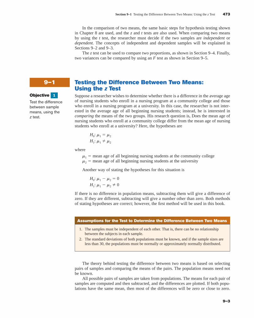
Occasionally, there will be a few large differences due to chance alone, some positive andothers negative. If the differences are plotted, the curve will be shaped like a normal dis-tribution and have a mean of zero, as shown in Figure 9–1.
The variance of the difference � is equal to the sum of the individual variancesof and . That is,
where
So the standard deviation of � is
As2
1
n1�s2
2
n2
X2X1
s 2X1
�s2
1
n1 and s2
X2�s2
2
n2
� s 2X1
� s 2X2
2X1� X2s
X2X1
X2X1
474 Chapter 9 Testing the Difference Between Two Means, Two Proportions, and Two Variances
9–4
Figure 9–1
Differences of Meansof Pairs of Samples
0
Distribution of X–1 � X–2
Unusual Stats
Adult children wholive with their parentsspend more than2 hours a day doinghousehold chores.According to a study,daughters contributeabout 17 hours aweek and sons about14.4 hours.
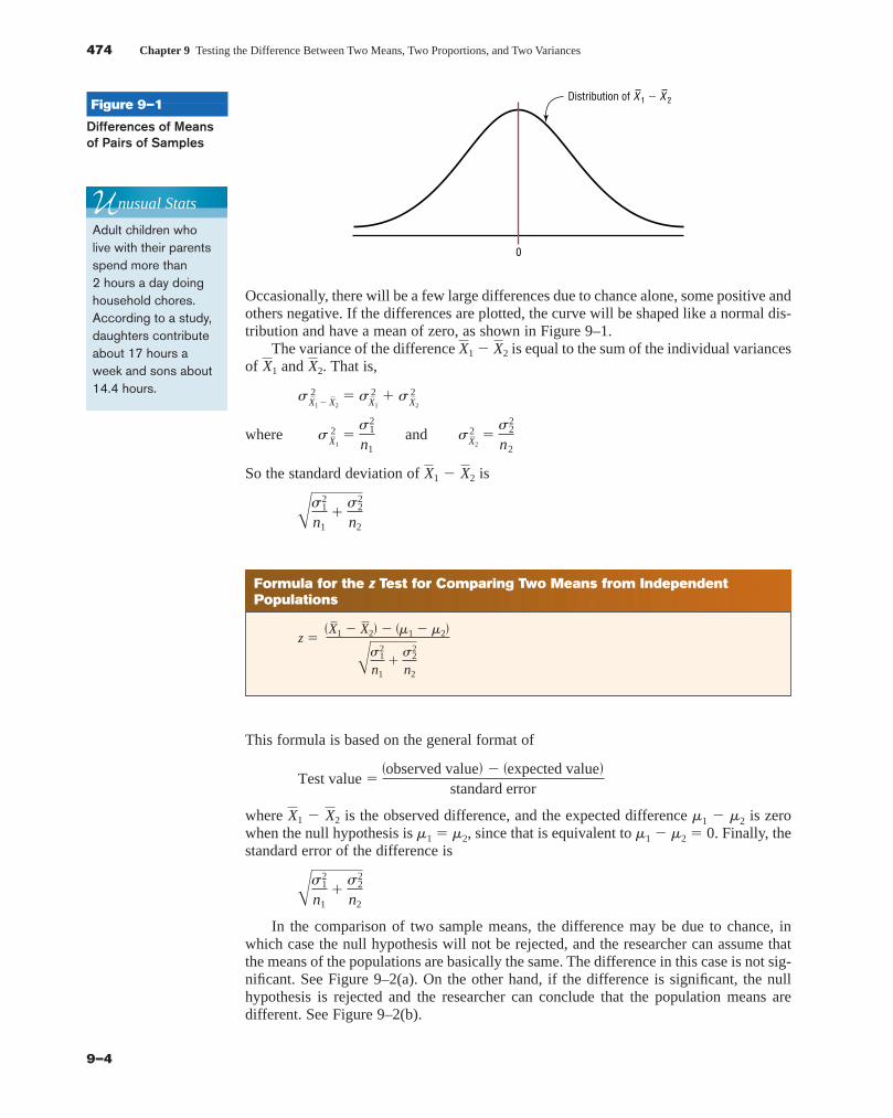
Formula for the z Test for Comparing Two Means from IndependentPopulations
z � �X1 � X2� � �m1 � m2�
As2
1
n1�s2
2
n2
This formula is based on the general format of
where � is the observed difference, and the expected difference m1 � m2 is zerowhen the null hypothesis is m1 � m2, since that is equivalent to m1 � m2 � 0. Finally, thestandard error of the difference is
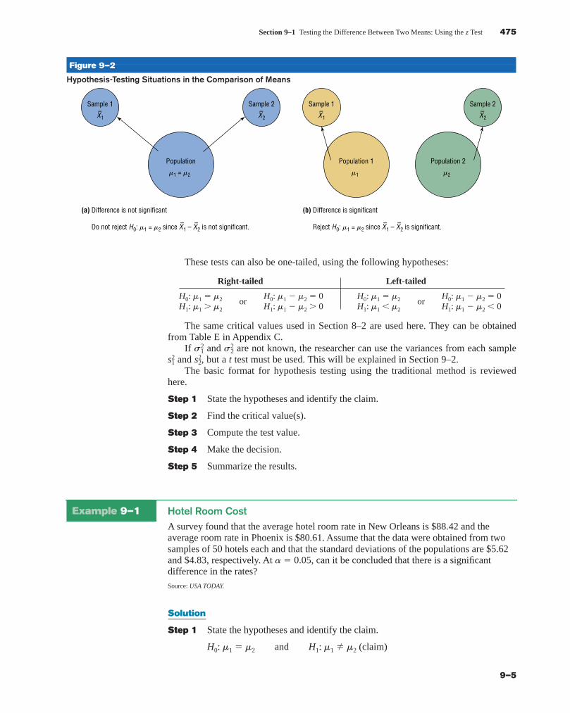
In the comparison of two sample means, the difference may be due to chance, inwhich case the null hypothesis will not be rejected, and the researcher can assume thatthe means of the populations are basically the same. The difference in this case is not sig-nificant. See Figure 9–2(a). On the other hand, if the difference is significant, the nullhypothesis is rejected and the researcher can conclude that the population means aredifferent. See Figure 9–2(b).
As2
1
n1�s2
2
n2
X2X1
Test value ��observed value� � �expected value�
standard error
blu34978_ch09.qxd 8/13/08 6:06 PM Page 474
Confirming Pages
These tests can also be one-tailed, using the following hypotheses:
Right-tailed Left-tailed
H0: m1 � m2 H0: m1 � m2 � 0 H0: m1 � m2 H0: m1 � m2 � 0H1: m1 � m2
orH1: m1 � m2 � 0 H1: m1 � m2
orH1: m1 � m2 � 0
The same critical values used in Section 8–2 are used here. They can be obtainedfrom Table E in Appendix C.
If and are not known, the researcher can use the variances from each sampleand , but a t test must be used. This will be explained in Section 9–2.
The basic format for hypothesis testing using the traditional method is reviewedhere.
Step 1 State the hypotheses and identify the claim.
Step 2 Find the critical value(s).
Step 3 Compute the test value.
Step 4 Make the decision.
Step 5 Summarize the results.
s22s2
1
s22s2
1
Section 9–1 Testing the Difference Between Two Means: Using the z Test 475
9–5
Sample 1
(a) Difference is not significant (b) Difference is significant
X–1
Population
�1 = �2
Sample 2
X–2
Sample 2
X–2
Sample 1
X–1
Reject H0: �1 = �2 since X–1 – X–2 is significant.Do not reject H0: �1 = �2 since X–1 – X–2 is not significant.
Population 2
�2
Population 1
�1
Figure 9–2
Hypothesis-Testing Situations in the Comparison of Means
Example 9–1 Hotel Room CostA survey found that the average hotel room rate in New Orleans is $88.42 and theaverage room rate in Phoenix is $80.61. Assume that the data were obtained from twosamples of 50 hotels each and that the standard deviations of the populations are $5.62and $4.83, respectively. At a � 0.05, can it be concluded that there is a significantdifference in the rates?Source: USA TODAY.
Solution
Step 1 State the hypotheses and identify the claim.
H0: m1 � m2 and H1: m1 � m2 (claim)
blu34978_ch09.qxd 8/13/08 6:06 PM Page 475
Confirming Pages
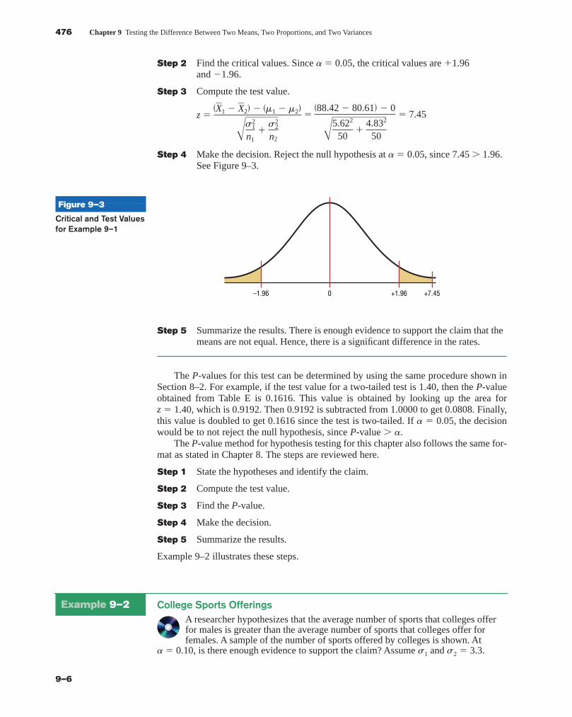
Step 2 Find the critical values. Since a � 0.05, the critical values are �1.96and �1.96.
Step 3 Compute the test value.
Step 4 Make the decision. Reject the null hypothesis at a � 0.05, since 7.45 � 1.96.See Figure 9–3.
z ��X1 � X2� � �m1 � m2�
As2
1
n1�s2
2
n2
��88.42 � 80.61� � 0
A5.622
50�
4.832
50
� 7.45
476 Chapter 9 Testing the Difference Between Two Means, Two Proportions, and Two Variances
9–6
Figure 9–3
Critical and Test Valuesfor Example 9–1
0 +7.45+1.96–1.96
Step 5 Summarize the results. There is enough evidence to support the claim that themeans are not equal. Hence, there is a significant difference in the rates.
The P-values for this test can be determined by using the same procedure shown inSection 8–2. For example, if the test value for a two-tailed test is 1.40, then the P-valueobtained from Table E is 0.1616. This value is obtained by looking up the area forz � 1.40, which is 0.9192. Then 0.9192 is subtracted from 1.0000 to get 0.0808. Finally,this value is doubled to get 0.1616 since the test is two-tailed. If a � 0.05, the decisionwould be to not reject the null hypothesis, since P-value � a.
The P-value method for hypothesis testing for this chapter also follows the same for-mat as stated in Chapter 8. The steps are reviewed here.
Step 1 State the hypotheses and identify the claim.
Step 2 Compute the test value.
Step 3 Find the P-value.
Step 4 Make the decision.
Step 5 Summarize the results.
Example 9–2 illustrates these steps.
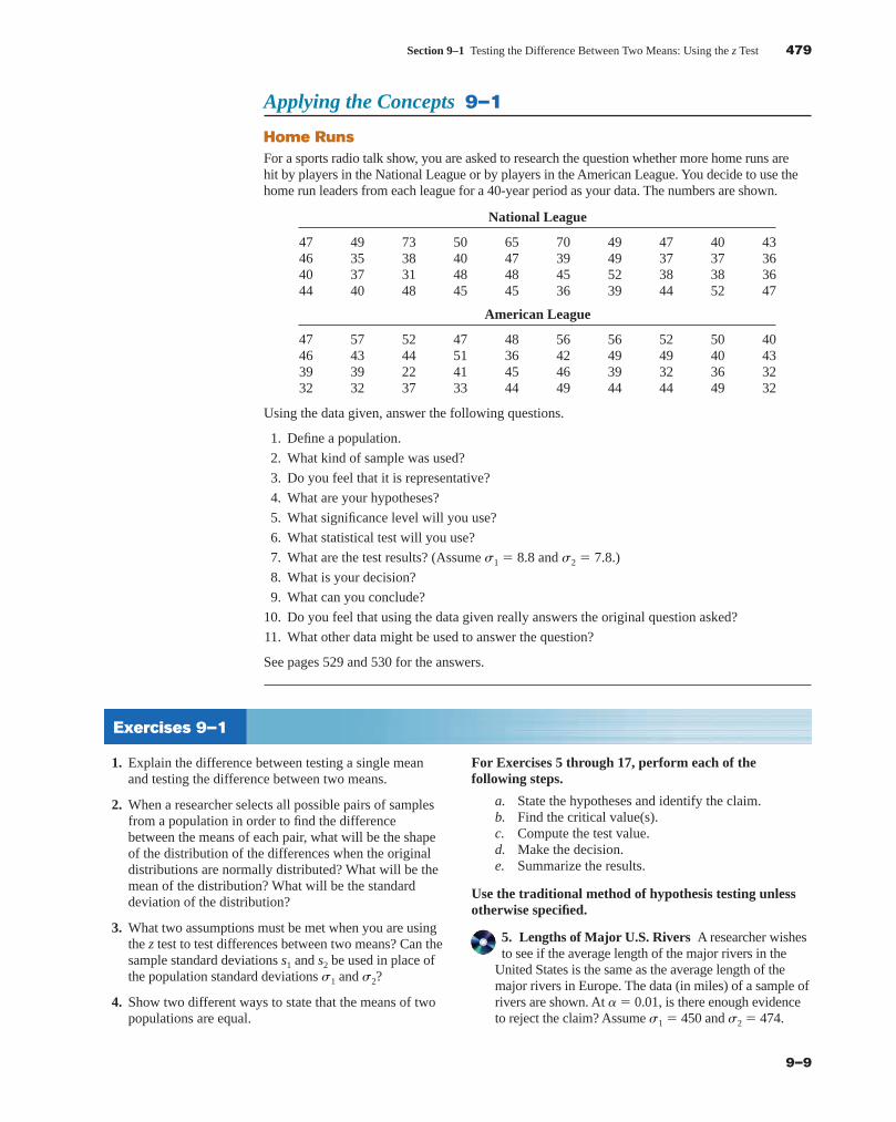
Example 9–2 College Sports OfferingsA researcher hypothesizes that the average number of sports that colleges offerfor males is greater than the average number of sports that colleges offer forfemales. A sample of the number of sports offered by colleges is shown. At
a � 0.10, is there enough evidence to support the claim? Assume s1 and s2 � 3.3.
blu34978_ch09.qxd 8/13/08 6:06 PM Page 476
Confirming Pages

Males Females
6 11 11 8 15 6 8 11 13 86 14 8 12 18 7 5 13 14 66 9 5 6 9 6 5 5 7 66 9 18 7 6 10 7 6 5 5
15 6 11 5 5 16 10 7 8 59 9 5 5 8 7 5 5 6 58 9 6 11 6 9 18 13 7 109 5 11 5 8 7 8 5 7 67 7 5 10 7 11 4 6 8 7
10 7 10 8 11 14 12 5 8 5Source: USA TODAY.
Solution
Step 1 State the hypotheses and identify the claim.
H0: m1 � m2 and H1: m1 � m2 (claim)
Step 2 Compute the test value. Using a calculator or the formula in Chapter 3, findthe mean for each data set.
For the males � 8.6 and s1 � 3.3
For the females � 7.9 and s2 � 3.3
Substitute in the formula.
Step 3 Find the P-value. For z � 1.06, the area is 0.8554, and 1.0000 � 0.8554 �0.1446, or a P-value of 0.1446.
Step 4 Make the decision. Since the P-value is larger than a (that is, 0.1446 � 0.10),the decision is to not reject the null hypothesis. See Figure 9–4.
Step 5 Summarize the results. There is not enough evidence to support the claim thatcolleges offer more sports for males than they do for females.
z � �X1 � X2� � �m1 � m2�
As2
1
n1�s2
2
n2
��8.6 � 7.9� � 0
A3.32
50�
3.32
50
� 1.06*
X2
X1
Section 9–1 Testing the Difference Between Two Means: Using the z Test 477
9–7
Figure 9–4
P-Value and A Value forExample 9–2
0
0.10
0.1446
*Note: Calculator results may differ due to rounding.
Sometimes, the researcher is interested in testing a specific difference in meansother than zero. For example, he or she might hypothesize that the nursing students at a
blu34978_ch09.qxd 8/13/08 6:06 PM Page 477
Confirming Pages
community college are, on average, 3.2 years older than those at a university. In this case,the hypotheses are
H0: m1 � m2 � 3.2 and H1: m1 � m2 � 3.2
The formula for the z test is still
wherem1 �m2 is the hypothesized difference or expected value. In this case,m1 �m2 � 3.2.Confidence intervals for the difference between two means can also be found. When
you are hypothesizing a difference of zero, if the confidence interval contains zero, thenull hypothesis is not rejected. If the confidence interval does not contain zero, the nullhypothesis is rejected.
Confidence intervals for the difference between two means can be found by usingthis formula:
z � �X1 � X2� � �m1 � m2�
As2
1
n1�s2
2
n2
478 Chapter 9 Testing the Difference Between Two Means, Two Proportions, and Two Variances
9–8
Formula for the z Confidence Interval for Difference Between Two Means
� �X1 � X2� � za�2As2
1
n 1�s2
2
n 2
�X1 � X2� � za�2As2
1
n 1�s2
2
n 2� m1 � m2
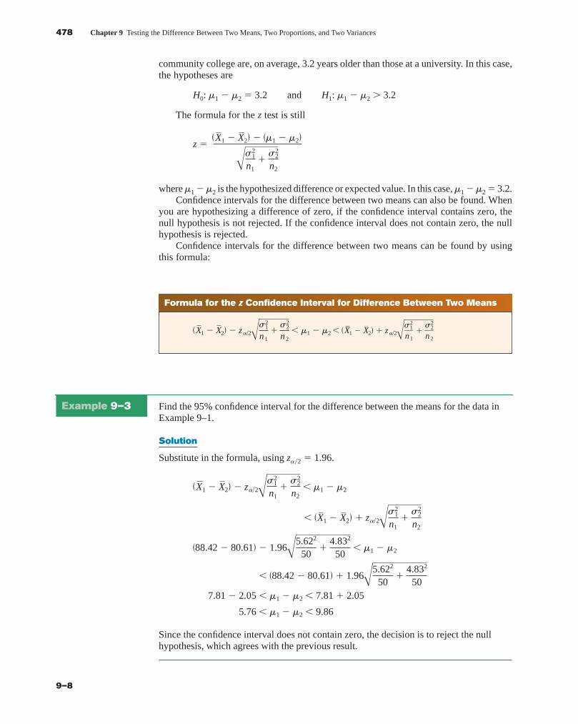
Example 9–3 Find the 95% confidence interval for the difference between the means for the data inExample 9–1.
Solution
Substitute in the formula, using za�2 � 1.96.
Since the confidence interval does not contain zero, the decision is to reject the nullhypothesis, which agrees with the previous result.
5.76 � m1 � m2 � 9.86
7.81 � 2.05 � m1 � m2 � 7.81 � 2.05
� �88.42 � 80.61� � 1.96A5.622
50�
4.832
50
�88.42 � 80.61� � 1.96A5.622
50�
4.832
50� m1 � m2
� �X1 � X2� � za�2As2
1
n1�s2
2
n2
�X1 � X2� � za�2As2
1
n1�s2
2
n2� m1 � m2
blu34978_ch09.qxd 8/13/08 6:06 PM Page 478
Confirming Pages
Applying the Concepts 9–1
Home RunsFor a sports radio talk show, you are asked to research the question whether more home runs arehit by players in the National League or by players in the American League. You decide to use thehome run leaders from each league for a 40-year period as your data. The numbers are shown.
National League
47 49 73 50 65 70 49 47 40 4346 35 38 40 47 39 49 37 37 3640 37 31 48 48 45 52 38 38 3644 40 48 45 45 36 39 44 52 47
American League
47 57 52 47 48 56 56 52 50 4046 43 44 51 36 42 49 49 40 4339 39 22 41 45 46 39 32 36 3232 32 37 33 44 49 44 44 49 32
Using the data given, answer the following questions.
1. Define a population.
2. What kind of sample was used?
3. Do you feel that it is representative?
4. What are your hypotheses?
5. What significance level will you use?
6. What statistical test will you use?
7. What are the test results? (Assume s1 � 8.8 and s2 � 7.8.)
8. What is your decision?
9. What can you conclude?
10. Do you feel that using the data given really answers the original question asked?
11. What other data might be used to answer the question?
See pages 529 and 530 for the answers.
Section 9–1 Testing the Difference Between Two Means: Using the z Test 479
9–9
1. Explain the difference between testing a single meanand testing the difference between two means.
2. When a researcher selects all possible pairs of samplesfrom a population in order to find the differencebetween the means of each pair, what will be the shapeof the distribution of the differences when the originaldistributions are normally distributed? What will be themean of the distribution? What will be the standarddeviation of the distribution?
3. What two assumptions must be met when you are usingthe z test to test differences between two means? Can thesample standard deviations s1 and s2 be used in place ofthe population standard deviations s1 and s2?
4. Show two different ways to state that the means of twopopulations are equal.
For Exercises 5 through 17, perform each of thefollowing steps.
a. State the hypotheses and identify the claim.b. Find the critical value(s).c. Compute the test value.d. Make the decision.e. Summarize the results.
Use the traditional method of hypothesis testing unlessotherwise specified.
5. Lengths of Major U.S. Rivers A researcher wishesto see if the average length of the major rivers in the
United States is the same as the average length of themajor rivers in Europe. The data (in miles) of a sample ofrivers are shown. At a� 0.01, is there enough evidenceto reject the claim? Assume s1 � 450 and s2 � 474.
Exercises 9–1
blu34978_ch09.qxd 8/13/08 6:06 PM Page 479
Confirming Pages
United States Europe
729 560 434 481 724 820329 332 360 532 357 505450 2315 865 1776 1122 496330 410 1036 1224 634 230329 800 447 1420 326 626600 1310 652 877 580 210
1243 605 360 447 567 252525 926 722 824 932 600850 310 430 634 1124 1575532 375 1979 565 405 2290710 545 259 675 454300 470 425
Source: The World Almanac and Book of Facts.
6. Wind Speeds The average wind speed in Casper,Wyoming, has been found to 12.7 miles per hour, and inPhoenix, Arizona, it is 6.2 miles per hour. To test therelationship between the averages, the average windspeed was calculated for a sample of 31 days for eachcity. The results are reported below. Is there sufficientevidence at a� 0.05 to conclude that the average windspeed is greater in Casper than in Phoenix?
Casper Phoenix
Sample size 31 31Sample mean 12.85 mph 7.9 mphPopulation standard deviation 3.3 mph 2.8 mphSource: World Almanac.
7. Commuting Times The Bureau of the Census reportsthat the average commuting time for citizens of bothBaltimore, Maryland, and Miami, Florida, is approxi-mately 29 minutes. To see if their commuting timesappear to be any different in the winter, random sam-ples of 40 drivers were surveyed in each city and theaverage commuting time for the month of January wascalculated for both cities. The results are providedbelow. At the 0.05 level of significance, can it beconcluded that the commuting times are different inthe winter?
Miami Baltimore
Sample size 40 40Sample mean 28.5 min 35.2 minPopulation standard deviation 7.2 min 9.1 minSource: www.census.gov
8. Heights of 9-Year-Olds At age 9 the average weight(21.3 kg) and the average height (124.5 cm) for bothboys and girls are exactly the same. A random sampleof 9-year-olds yielded these results. Estimate the meandifference in height between boys and girls with 95%confidence. Does your interval support the given claim?
Boys Girls
Sample size 60 50Mean height, cm 123.5 126.2Population variance 98 120Source: www.healthepic.com
9. Length of Hospital Stays The average length of“short hospital stays” for men is slightly longer thanthat for women, 5.2 days versus 4.5 days. A randomsample of recent hospital stays for both men andwomen revealed the following. At a � 0.01, is theresufficient evidence to conclude that the average hospitalstay for men is longer than the average hospital stay forwomen?
Men Women
Sample size 32 30Sample mean 5.5 days 4.2 daysPopulation standard deviation 1.2 days 1.5 days
Source: www.cdc.gov/nchs
10. Home Prices A real estate agent compares the sellingprices of homes in two municipalities in southwesternPennsylvania to see if there is a difference. The resultsof the study are shown. Is there enough evidence toreject the claim that the average cost of a home in bothlocations is the same? Use a � 0.01.
Scott Ligonier
*Based on information from RealSTATs.
11. Women Science Majors In a study of women sciencemajors, the following data were obtained on twogroups, those who left their profession within a fewmonths after graduation (leavers) and those whoremained in their profession after they graduated(stayers). Test the claim that those who stayed had ahigher science grade point average than those who left.Use a � 0.05.
Leavers Stayers
� 3.16 � 3.28s1 � 0.52 s2 � 0.46n1 � 103 n2 � 225
Source: Paula Rayman and Belle Brett, “Women Science Majors: What Makes a Difference in Persistence after Graduation?” The Journal of Higher Education.
12. ACT Scores A survey of 1000 students nationwideshowed a mean ACT score of 21.4. A survey of 500Ohio scores showed a mean of 20.8. If the populationstandard deviation in each case is 3, can we concludethat Ohio is below the national average? Use a � 0.05.
Source: Report of WFIN radio.
13. Money Spent on College Sports A schooladministrator hypothesizes that colleges spend more
for male sports than they do for female sports. A sampleof two different colleges is selected, and the annualexpenses (in dollars) per student at each school areshown. At a � 0.01, is there enough evidence tosupport the claim? Assume s1 � 3830 and s2 � 2745.
X2X1
n2 � 40n 1 � 35s2 � $4731s1 � $5602X2 � $98,043*X1 � $93,430*
480 Chapter 9 Testing the Difference Between Two Means, Two Proportions, and Two Variances
9–10
blu34978_ch09.qxd 8/13/08 6:06 PM Page 480
Confirming Pages
Males
7,040 6,576 1,664 12,919 8,60522,220 3,377 10,128 7,723 2,0638,033 9,463 7,656 11,456 12,2446,670 12,371 9,626 5,472 16,1758,383 623 6,797 10,160 8,725
14,029 13,763 8,811 11,480 9,54415,048 5,544 10,652 11,267 10,1268,796 13,351 7,120 9,505 9,5717,551 5,811 9,119 9,732 5,2865,254 7,550 11,015 12,403 12,703
Females
10,333 6,407 10,082 5,933 3,9917,435 8,324 6,989 16,249 5,9227,654 8,411 11,324 10,248 6,0309,331 6,869 6,502 11,041 11,5975,468 7,874 9,277 10,127 13,3717,055 6,909 8,903 6,925 7,058
12,745 12,016 9,883 14,698 9,9078,917 9,110 5,232 6,959 5,8327,054 7,235 11,248 8,478 6,5027,300 993 6,815 9,959 10,353
Source: USA TODAY.
14. Monthly Social Security Benefits The averagemonthly Social Security benefit in 2004 for retiredworkers was $954.90 and for disabled workers was$894.10. Researchers used data from the Social Securityrecords to test the claim that the difference in monthlybenefits between the two groups was greater than $30.Based on the following information, can theresearchers’ claim be supported at the 0.05 level ofsignificance?
Retired Disabled
Sample size 60 60Mean benefit $960.50 $902.89Population standard deviation $98 $101
Source: New York Times Almanac.
15. Self-Esteem Scores In the study cited in Exercise 11,the researchers collected the data shown here on a self-esteem questionnaire. At a � 0.05, can it be concludedthat there is a difference in the self-esteem scores of thetwo groups? Use the P-value method.
Leavers Stayers
� 3.05 � 2.96s1 � 0.75 s2 � 0.75n1 � 103 n2 � 225Source: Paula Rayman and Belle Brett, “Women Science Majors: What Makes a Difference in Persistence after Graduation?” The Journal of Higher Education.
16. Ages of College Students The dean of studentswants to see whether there is a significant difference in
ages of resident students and commuting students. Sheselects a sample of 50 students from each group. The agesare shown here. At a� 0.05, decide if there is enough
X2X1
evidence to reject the claim of no difference in the agesof the two groups. Use the standard deviations from thesamples and the P-value method. Assume s1 � 3.68 ands2 � 4.7.
Resident students
22 25 27 23 26 28 26 2425 20 26 24 27 26 18 1918 30 26 18 18 19 32 2319 19 18 29 19 22 18 2226 19 19 21 23 18 20 1822 21 19 21 21 22 18 2019 23
Commuter students
18 20 19 18 22 25 24 3523 18 23 22 28 25 20 2426 30 22 22 22 21 18 2019 26 35 19 19 18 19 3229 23 21 19 36 27 27 2020 21 18 19 23 20 19 1920 25
17. Problem-Solving Ability Two groups of students aregiven a problem-solving test, and the results are com-pared. Find the 90% confidence interval of the truedifference in means.
Mathematics majors Computer science majors
� 83.6 � 79.2s1 � 4.3 s2 � 3.8n1 � 36 n2 � 36
18. Credit Card Debt The average credit card debt for arecent year was $9205. Five years earlier the averagecredit card debt was $6618. Assume sample sizes of 35were used and the population standard deviations ofboth samples were $1928. Is there enough evidence tobelieve that the average credit card debt has increased?Use a � 0.05. Give a possible reason as to why or whynot the debt was increased.Source: CardWeb.com
19. Literacy Scores Adults aged 16 or older were assessedin three types of literacy in 2003: prose, document, andquantitative. The scores in document literacy were thesame for 19- to 24-year-olds and for 40- to 49-year-olds.A random sample of scores from a later year showed thefollowing statistics.
Population Mean standard Sample
Age group score deviation size
19–24 280 56.2 4040–49 315 52.1 35
Construct a 95% confidence interval for the truedifference in mean scores for these two groups. Whatdoes your interval say about the claim that there is nodifference in mean scores?Source: www.nces.ed.gov
X2X1
Section 9–1 Testing the Difference Between Two Means: Using the z Test 481
9–11
blu34978_ch09.qxd 8/13/08 6:06 PM Page 481
Confirming Pages
482 Chapter 9 Testing the Difference Between Two Means, Two Proportions, and Two Variances
9–12
21. Exam Scores at Private and Public Schools A re-searcher claims that students in a private school haveexam scores that are at most 8 points higher than thoseof students in public schools. Random samples of 60 stu-dents from each type of school are selected and given anexam. The results are shown. At a� 0.05, test the claim.
Extending the ConceptsPrivate school Public school
� 110 � 104s1 � 15 s2 � 15n1 � 60 n2 � 60
X2X1
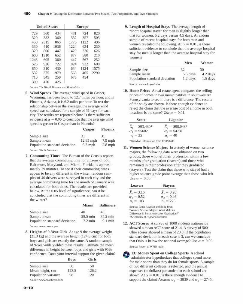
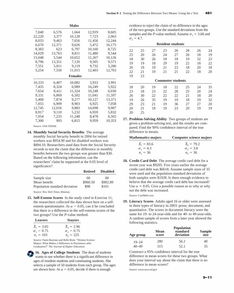
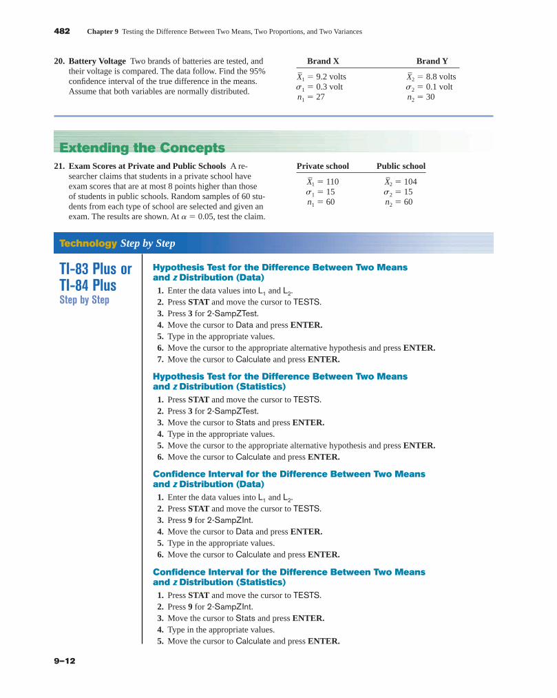
Hypothesis Test for the Difference Between Two Means and z Distribution (Data)1. Enter the data values into L1 and L2.2. Press STAT and move the cursor to TESTS.3. Press 3 for 2-SampZTest.4. Move the cursor to Data and press ENTER.5. Type in the appropriate values.6. Move the cursor to the appropriate alternative hypothesis and press ENTER.7. Move the cursor to Calculate and press ENTER.
Hypothesis Test for the Difference Between Two Means and z Distribution (Statistics)1. Press STAT and move the cursor to TESTS.2. Press 3 for 2-SampZTest.3. Move the cursor to Stats and press ENTER.4. Type in the appropriate values.5. Move the cursor to the appropriate alternative hypothesis and press ENTER.6. Move the cursor to Calculate and press ENTER.
Confidence Interval for the Difference Between Two Means and z Distribution (Data)1. Enter the data values into L1 and L2.2. Press STAT and move the cursor to TESTS.3. Press 9 for 2-SampZInt.4. Move the cursor to Data and press ENTER.5. Type in the appropriate values.6. Move the cursor to Calculate and press ENTER.
Confidence Interval for the Difference Between Two Means and z Distribution (Statistics)1. Press STAT and move the cursor to TESTS.2. Press 9 for 2-SampZInt.3. Move the cursor to Stats and press ENTER.4. Type in the appropriate values.5. Move the cursor to Calculate and press ENTER.
Technology Step by Step
TI-83 Plus orTI-84 PlusStep by Step
20. Battery Voltage Two brands of batteries are tested, andtheir voltage is compared. The data follow. Find the 95%confidence interval of the true difference in the means.Assume that both variables are normally distributed.
Brand X Brand Y
� 9.2 volts � 8.8 voltss1 � 0.3 volt s2 � 0.1 voltn1 � 27 n2 � 30
X2X1
blu34978_ch09.qxd 8/13/08 6:06 PM Page 482
Confirming Pages
Section 9–1 Testing the Difference Between Two Means: Using the z Test 483
9–13
ExcelStep by Step
z Test for the Difference Between Two MeansExcel has a two-sample z test included in the Data Analysis Add-in. To perform a z test for thedifference between the means of two populations, given two independent samples, do this:
1. Enter the first sample data set into column A.
2. Enter the second sample data set into column B.
3. If the population variances are not known but n � 30 for both samples, use the formulas=VAR(A1:An) and =VAR(B1:Bn), where An and Bn are the last cells with data in eachcolumn, to find the variances of the sample data sets.
4. Select the Data tab from the toolbar. Then select Data Analysis.
5. In the Analysis Tools box, select z test: Two sample for Means.
6. Type the ranges for the data in columns A and B and type a value (usually 0) for theHypothesized Mean Difference.
7. If the population variances are known, type them for Variable 1 and Variable 2. Otherwise,use the sample variances obtained in step 3.
8. Specify the confidence level Alpha.
9. Specify a location for the output, and click [OK].
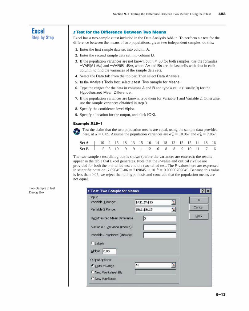
Example XL9–1
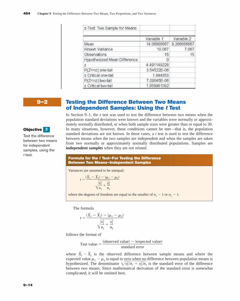
Test the claim that the two population means are equal, using the sample data providedhere, at a� 0.05. Assume the population variances are � 10.067 and � 7.067.
Set A 10 2 15 18 13 15 16 14 18 12 15 15 14 18 16
Set B 5 8 10 9 9 11 12 16 8 8 9 10 11 7 6
The two-sample z test dialog box is shown (before the variances are entered); the resultsappear in the table that Excel generates. Note that the P-value and critical z value areprovided for both the one-tailed test and the two-tailed test. The P-values here are expressedin scientific notation: 7.09045E-06 � 7.09045 10�6 � 0.00000709045. Because this valueis less than 0.05, we reject the null hypothesis and conclude that the population means arenot equal.
s 2Bs 2
A
Two-Sample z TestDialog Box
blu34978_ch09.qxd 8/13/08 6:06 PM Page 483
Confirming Pages
484 Chapter 9 Testing the Difference Between Two Means, Two Proportions, and Two Variances
9–14
9–2 Testing the Difference Between Two Meansof Independent Samples: Using the t TestIn Section 9–1, the z test was used to test the difference between two means when thepopulation standard deviations were known and the variables were normally or approxi-mately normally distributed, or when both sample sizes were greater than or equal to 30.In many situations, however, these conditions cannot be met—that is, the populationstandard deviations are not known. In these cases, a t test is used to test the differencebetween means when the two samples are independent and when the samples are takenfrom two normally or approximately normally distributed populations. Samples areindependent samples when they are not related.
Objective
Test the differencebetween two meansfor independentsamples, using thet test.
2
Formula for the t Test—For Testing the Difference Between Two Means—Independent Samples
Variances are assumed to be unequal:
where the degrees of freedom are equal to the smaller of n1 � 1 or n2 � 1.
t � �X1 � X2� � �m1 � m2�
As2
1
n1�
s22
n2
The formula
follows the format of
where � is the observed difference between sample means and where theexpected value m1 � m2 is equal to zero when no difference between population means ishypothesized. The denominator is the standard error of the differencebetween two means. Since mathematical derivation of the standard error is somewhatcomplicated, it will be omitted here.
2s12 n1 � s2
2 n2
X2X1
Test value ��observed value� � �expected value�
standard error
t � �X1 � X2� � �m1 � m2�
As2
1
n1�
s22
n2
blu34978_ch09.qxd 8/13/08 6:06 PM Page 484
Confirming Pages
Section 9–2 Testing the Difference Between Two Means of Independent Samples: Using the t Test 485
9–15
Example 9–4 Farm SizesThe average size of a farm in Indiana County, Pennsylvania, is 191 acres. The average sizeof a farm in Greene County, Pennsylvania, is 199 acres. Assume the data were obtainedfrom two samples with standard deviations of 38 and 12 acres, respectively, and samplesizes of 8 and 10, respectively. Can it be concluded at a� 0.05 that the average size of thefarms in the two counties is different? Assume the populations are normally distributed.Source: Pittsburgh Tribune-Review.
Solution
Step 1 State the hypotheses and identify the claim for the means.
H0: m1 � m2 and H1: m1 � m2 (claim)
Step 2 Find the critical values. Since the test is two-tailed, since a � 0.05, and sincethe variances are unequal, the degrees of freedom are the smaller of n1 � 1or n2 � 1. In this case, the degrees of freedom are 8 � 1 � 7. Hence, fromTable F, the critical values are �2.365 and �2.365.
Step 3 Compute the test value. Since the variances are unequal, use the first formula.
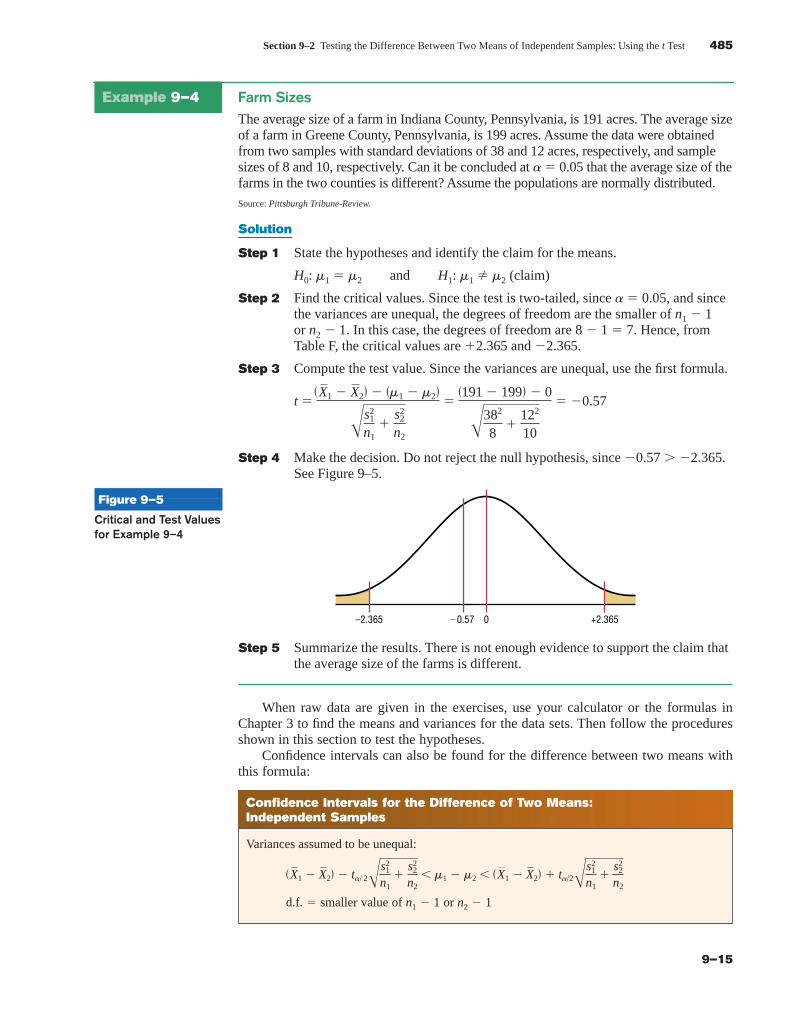
Step 4 Make the decision. Do not reject the null hypothesis, since �0.57 � �2.365.See Figure 9–5.
t � �X1 � X2� � �m1 � m2�
As2
1
n1�
s22
n2
��191 � 199� � 0
A382
8�
122
10
� �0.57
Figure 9–5
Critical and Test Valuesfor Example 9–4
0 +2.365�0.57–2.365
Confidence Intervals for the Difference of Two Means: Independent Samples
Variances assumed to be unequal:
d.f. � smaller value of n1 � 1 or n2 � 1
�X1 � X2� � ta� 2As2
1
n1�
s22
n2� m1 � m2 � �X1 � X2� � ta�2A
s21
n1�
s22
n2
Step 5 Summarize the results. There is not enough evidence to support the claim thatthe average size of the farms is different.
When raw data are given in the exercises, use your calculator or the formulas inChapter 3 to find the means and variances for the data sets. Then follow the proceduresshown in this section to test the hypotheses.
Confidence intervals can also be found for the difference between two means withthis formula:
blu34978_ch09.qxd 8/13/08 6:06 PM Page 485
Confirming Pages
486 Chapter 9 Testing the Difference Between Two Means, Two Proportions, and Two Variances
9–16
Example 9–5 Find the 95% confidence interval for the data in Example 9–4.
Solution
Substitute in the formula.
Since 0 is contained in the interval, the decision is to not reject the null hypothesis H0: m1 � m2.
In many statistical software packages, a different method is used to compute thedegrees of freedom for this t test. They are determined by the formula
This formula will not be used in this textbook.There are actually two different options for the use of t tests. One option is used when
the variances of the populations are not equal, and the other option is used when the vari-ances are equal. To determine whether two sample variances are equal, the researchercan use an F test, as shown in Section 9–5.
When the variances are assumed to be equal, this formula is used and
follows the format of
For the numerator, the terms are the same as in the previously given formula. However,a note of explanation is needed for the denominator of the second test statistic. Since bothpopulations are assumed to have the same variance, the standard error is computed withwhat is called a pooled estimate of the variance. A pooled estimate of the variance isa weighted average of the variance using the two sample variances and the degrees offreedom of each variance as the weights. Again, since the algebraic derivation of thestandard error is somewhat complicated, it is omitted.
Note, however, that not all statisticians are in agreement about using the F test beforeusing the t test. Some believe that conducting the F and t tests at the same level of sig-nificance will change the overall level of significance of the t test. Their reasons arebeyond the scope of this textbook. Because of this, we will assume that s1 � s2 in thistextbook.
Test value ��observed value� � �expected value�
standard error
t � �X1 � X2� � �m1 � m2�
A�n1 � 1�s2
1 � �n2 � 1�s22
n1 � n2 � 2 A
1n1
�1n2
d.f. ��s2
1�n1 � s22�n2�2
�s21�n1�2��n1 � 1� � �s2
2�n2�2��n2 � 1�
�41.02 � m1 � m2 � 25.02
� �191 � 199� � 2.365A382
8�
122
10
�191 � 199� � 2.365A382
8�
122
10� m1 � m2
� �X1 � X2� � ta2As2
1
n1�
s22
n2
�X1 � X2� � ta2As2
1
n1�
s22
n2� m1 � m2
blu34978_ch09.qxd 8/13/08 6:06 PM Page 486
Confirming Pages
Section 9–2 Testing the Difference Between Two Means of Independent Samples: Using the t Test 487
9–17
Applying the Concepts 9–2
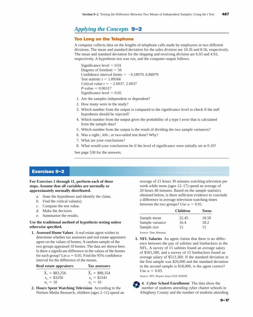
Too Long on the TelephoneA company collects data on the lengths of telephone calls made by employees in two differentdivisions. The mean and standard deviation for the sales division are 10.26 and 8.56, respectively.The mean and standard deviation for the shipping and receiving division are 6.93 and 4.93,respectively. A hypothesis test was run, and the computer output follows.
Significance level � 0.01Degrees of freedom � 56Confidence interval limits � �0.18979, 6.84979Test statistic t � 1.89566Critical value t � �2.0037, 2.0037P-value � 0.06317Significance level � 0.05
1. Are the samples independent or dependent?2. How many were in the study?3. Which number from the output is compared to the significance level to check if the null
hypothesis should be rejected?4. Which number from the output gives the probability of a type I error that is calculated
from the sample data?5. Which number from the output is the result of dividing the two sample variances?6. Was a right-, left-, or two-tailed test done? Why?7. What are your conclusions?8. What would your conclusions be if the level of significance were initially set at 0.10?
See page 530 for the answers.
For Exercises 1 through 11, perform each of thesesteps. Assume that all variables are normally orapproximately normally distributed.
a. State the hypotheses and identify the claim.b. Find the critical value(s).c. Compute the test value.d. Make the decision.e. Summarize the results.
Use the traditional method of hypothesis testing unlessotherwise specified.
1. Assessed Home Values A real estate agent wishes todetermine whether tax assessors and real estate appraisersagree on the values of homes. A random sample of thetwo groups appraised 10 homes. The data are shown here.Is there a significant difference in the values of the homesfor each group? Let a� 0.05. Find the 95% confidenceinterval for the difference of the means.
Real estate appraisers Tax assessors
� $83,256 � $88,354s1 � $3256 s2 � $2341n1 � 10 n2 � 10
2. Hours Spent Watching Television According to theNielsen Media Research, children (ages 2–11) spend an
X2X1
average of 21 hours 30 minutes watching television perweek while teens (ages 12–17) spend an average of20 hours 40 minutes. Based on the sample statisticsobtained below, is there sufficient evidence to concludea difference in average television watching timesbetween the two groups? Use a � 0.01.
Children Teens
Sample mean 22.45 18.50Sample variance 16.4 18.2Sample size 15 15Source: Time Almanac.
3. NFL Salaries An agent claims that there is no differ-ence between the pay of safeties and linebackers in theNFL. A survey of 15 safeties found an average salaryof $501,580, and a survey of 15 linebackers found anaverage salary of $513,360. If the standard deviation inthe first sample was $20,000 and the standard deviationin the second sample is $18,000, is the agent correct?Use a � 0.05.Source: NFL Players Assn./USA TODAY.
4. Cyber School Enrollment The data show thenumber of students attending cyber charter schools in
Allegheny County and the number of students attending
Exercises 9–2
blu34978_ch09.qxd 8/13/08 6:06 PM Page 487
Confirming Pages
488 Chapter 9 Testing the Difference Between Two Means, Two Proportions, and Two Variances
9–18
cyber schools in counties surrounding AlleghenyCounty. At a� 0.01 is there enough evidence to supportthe claim that the average number of students in schooldistricts in Allegheny County who attend cyber schoolsis greater than those who attend cyber schools in schooldistricts outside Allegheny County? Give a factor thatshould be considered in interpreting this answer.
Allegheny County Outside Allegheny County
25 75 38 41 27 32 57 25 38 14 10 29Source: Pittsburgh Tribune-Review.
5. Ages of Homes Whiting, Indiana, leads the “Top 100Cities with the Oldest Houses” list with the average ageof houses being 66.4 years. Farther down the list residesFranklin, Pennsylvania, with an average house age of59.4 years. Researchers selected a random sample of 20houses in each city and obtained the following statistics.At a � 0.05, can it be concluded that the houses inWhiting are older? Use the P-value method.
Whiting Franklin
Mean age 62.1 years 55.6 yearsStandard deviation 5.4 years 3.9 years
Source: www.city-data.com
6. Missing Persons A researcher wishes to test theclaim that, on average, more juveniles than adults are
classified as missing persons. Records for the last5 years are shown. At a � 0.10, is there enoughevidence to support the claim?
Juveniles 65,513 65,934 64,213 61,954 59,167
Adults 31,364 34,478 36,937 35,946 38,209
Source: USA TODAY.
7. IRS Tax Return Help The local branch of the InternalRevenue Service spent an average of 21 minuteshelping each of 10 people prepare their tax returns.The standard deviation was 5.6 minutes. A volunteertax preparer spent an average of 27 minutes helping14 people prepare their taxes. The standard deviationwas 4.3 minutes. At a � 0.02, is there a difference inthe average time spent by the two services? Find the98% confidence interval for the two means.
8. Volunteer Work of College Students Females andmales alike from the general adult population volunteeran average of 4.2 hours per week. A random sample of20 female college students and 18 male college studentsindicated these results concerning the amount of timespent in volunteer service per week. At the 0.01 level ofsignificance, is there sufficient evidence to conclude thata difference exists between the mean number of volunteerhours per week for male and female college students?
Male Female
Sample mean 2.5 3.8Sample variance 2.2 3.5Sample size 18 20Source: New York Times Almanac.
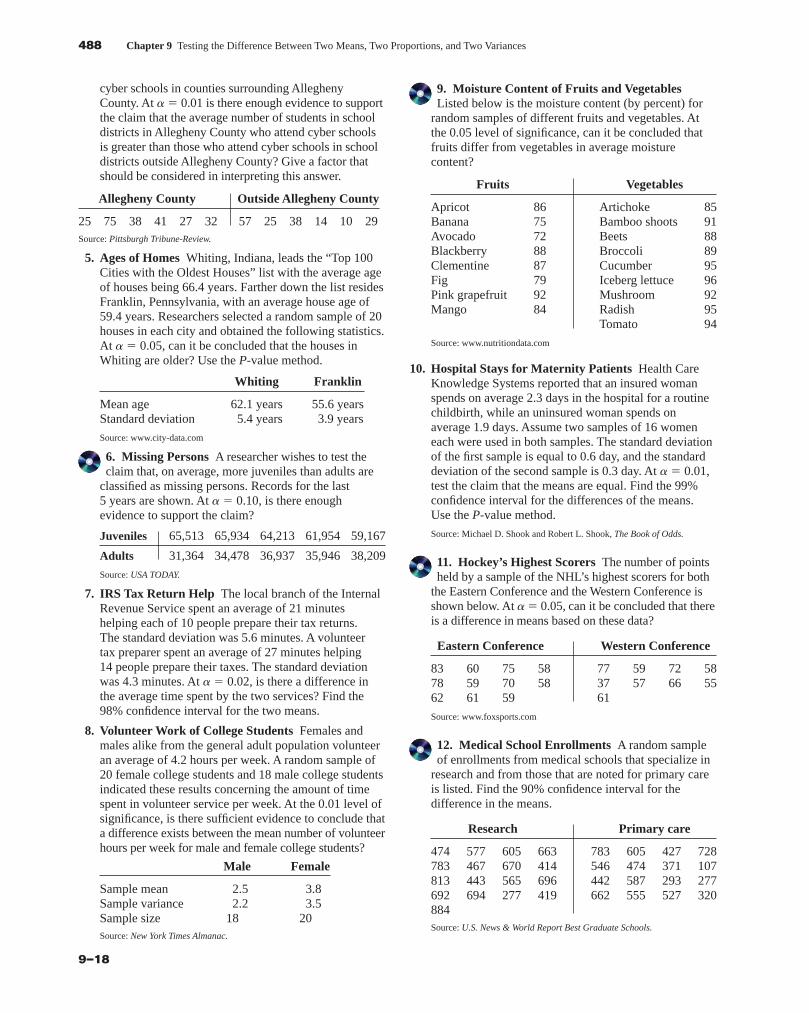
9. Moisture Content of Fruits and VegetablesListed below is the moisture content (by percent) for
random samples of different fruits and vegetables. Atthe 0.05 level of significance, can it be concluded thatfruits differ from vegetables in average moisturecontent?
Fruits Vegetables
Apricot 86 Artichoke 85Banana 75 Bamboo shoots 91Avocado 72 Beets 88Blackberry 88 Broccoli 89Clementine 87 Cucumber 95Fig 79 Iceberg lettuce 96Pink grapefruit 92 Mushroom 92Mango 84 Radish 95
Tomato 94
Source: www.nutritiondata.com
10. Hospital Stays for Maternity Patients Health CareKnowledge Systems reported that an insured womanspends on average 2.3 days in the hospital for a routinechildbirth, while an uninsured woman spends onaverage 1.9 days. Assume two samples of 16 womeneach were used in both samples. The standard deviationof the first sample is equal to 0.6 day, and the standarddeviation of the second sample is 0.3 day. At a � 0.01,test the claim that the means are equal. Find the 99%confidence interval for the differences of the means.Use the P-value method.
Source: Michael D. Shook and Robert L. Shook, The Book of Odds.
11. Hockey’s Highest Scorers The number of pointsheld by a sample of the NHL’s highest scorers for both
the Eastern Conference and the Western Conference isshown below. At a� 0.05, can it be concluded that thereis a difference in means based on these data?
Eastern Conference Western Conference
83 60 75 58 77 59 72 5878 59 70 58 37 57 66 5562 61 59 61
Source: www.foxsports.com
12. Medical School Enrollments A random sampleof enrollments from medical schools that specialize in
research and from those that are noted for primary careis listed. Find the 90% confidence interval for thedifference in the means.
Research Primary care
474 577 605 663 783 605 427 728783 467 670 414 546 474 371 107813 443 565 696 442 587 293 277692 694 277 419 662 555 527 320884Source: U.S. News & World Report Best Graduate Schools.
blu34978_ch09.qxd 8/13/08 6:44 PM Page 488
Confirming Pages
Section 9–2 Testing the Difference Between Two Means of Independent Samples: Using the t Test 489
9–19
13. Out-of-State Tuitions The out-of-state tuitions(in dollars) for random samples of both public and
private four-year colleges in a New England state arelisted. Find the 95% confidence interval for thedifference in the means.
Private Public
13,600 13,495 7,050 9,00016,590 17,300 6,450 9,75823,400 12,500 7,050 7,871
16,100Source: New York Times Almanac.
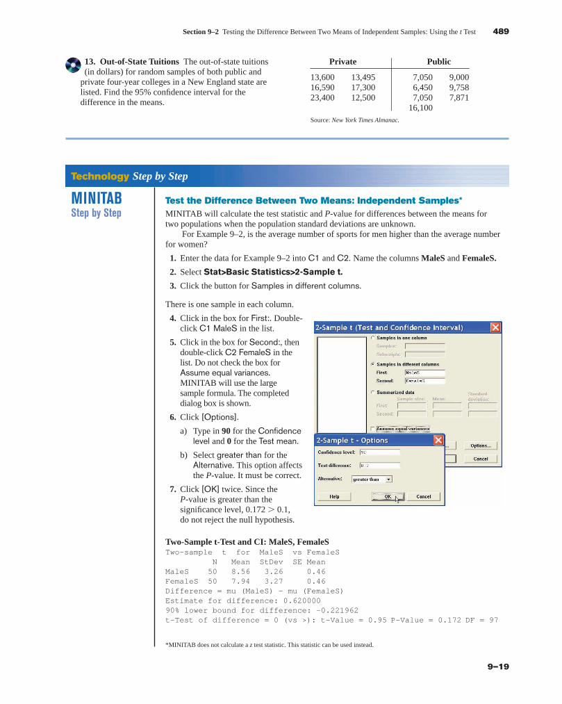
Test the Difference Between Two Means: Independent Samples*MINITAB will calculate the test statistic and P-value for differences between the means fortwo populations when the population standard deviations are unknown.
For Example 9–2, is the average number of sports for men higher than the average numberfor women?
1. Enter the data for Example 9–2 into C1 and C2. Name the columns MaleS and FemaleS.
2. Select Stat>Basic Statistics>2-Sample t.
3. Click the button for Samples in different columns.
There is one sample in each column.
4. Click in the box for First:. Double-click C1 MaleS in the list.
5. Click in the box for Second:, thendouble-click C2 FemaleS in thelist. Do not check the box forAssume equal variances.MINITAB will use the largesample formula. The completeddialog box is shown.
6. Click [Options].
a) Type in 90 for the Confidencelevel and 0 for the Test mean.
b) Select greater than for theAlternative. This option affectsthe P-value. It must be correct.
7. Click [OK] twice. Since theP-value is greater than thesignificance level, 0.172 � 0.1,do not reject the null hypothesis.
Two-Sample t-Test and CI: MaleS, FemaleSTwo-sample t for MaleS vs FemaleS
N Mean StDev SE MeanMaleS 50 8.56 3.26 0.46FemaleS 50 7.94 3.27 0.46Difference = mu (MaleS) - mu (FemaleS)Estimate for difference: 0.62000090% lower bound for difference: -0.221962t-Test of difference = 0 (vs >): t-Value = 0.95 P-Value = 0.172 DF = 97
Technology Step by Step
MINITABStep by Step
*MINITAB does not calculate a z test statistic. This statistic can be used instead.
blu34978_ch09.qxd 8/13/08 6:44 PM Page 489
Confirming Pages
490 Chapter 9 Testing the Difference Between Two Means, Two Proportions, and Two Variances
9–20
TI-83 Plus orTI-84 PlusStep by Step
Hypothesis Test for the Difference Between Two Means and t Distribution (Statistics)
1. Press STAT and move the cursor to TESTS.2. Press 4 for 2-SampTTest.3. Move the cursor to Stats and press ENTER.
4. Type in the appropriate values.
5. Move the cursor to the appropriate alternative hypothesis and press ENTER.
6. On the line for Pooled, move the cursor to No (standard deviations are assumed not equal)and press ENTER.
7. Move the cursor to Calculate and press ENTER.
Confidence Interval for the Difference Between Two Means and t Distribution (Data)
1. Enter the data values into L1 and L2.2. Press STAT and move the cursor to TESTS.3. Press 0 for 2-SampTInt.4. Move the cursor to Data and press ENTER.
5. Type in the appropriate values.
6. On the line for Pooled, move the cursor to No (standard deviations are assumed not equal)and press ENTER.
7. Move the cursor to Calculate and press ENTER.
Confidence Interval for the Difference Between Two Means and t Distribution (Statistics)
1. Press STAT and move the cursor to TESTS.2. Press 0 for 2-SampTInt.3. Move the cursor to Stats and press ENTER.
4. Type in the appropriate values.
5. On the line for Pooled, move the cursor to No (standard deviations are assumed not equal)and press ENTER.
6. Move the cursor to Calculate and press ENTER.
ExcelStep by Step
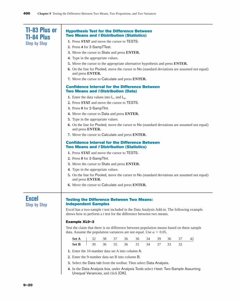
Testing the Difference Between Two Means: Independent SamplesExcel has a two-sample t test included in the Data Analysis Add-in. The following exampleshows how to perform a t test for the difference between two means.
Example XL9–2
Test the claim that there is no difference between population means based on these sampledata. Assume the population variances are not equal. Use a � 0.05.
Set A 32 38 37 36 36 34 39 36 37 42
Set B 30 36 35 36 31 34 37 33 32
1. Enter the 10-number data set A into column A.
2. Enter the 9-number data set B into column B.
3. Select the Data tab from the toolbar. Then select Data Analysis.
4. In the Data Analysis box, under Analysis Tools select t-test: Two-Sample AssumingUnequal Variances, and click [OK].
blu34978_ch09.qxd 8/13/08 6:06 PM Page 490
Confirming Pages
Section 9–3 Testing the Difference Between Two Means: Dependent Samples 491
9–21
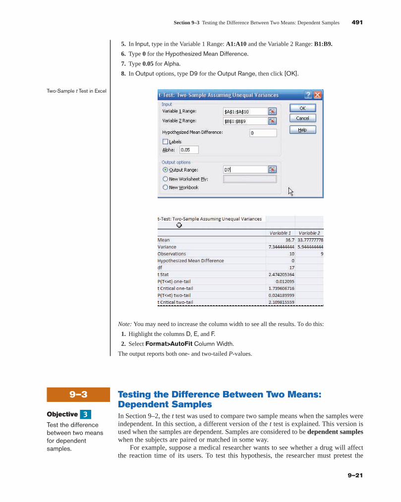
5. In Input, type in the Variable 1 Range: A1:A10 and the Variable 2 Range: B1:B9.
6. Type 0 for the Hypothesized Mean Difference.
7. Type 0.05 for Alpha.
8. In Output options, type D9 for the Output Range, then click [OK].
Note: You may need to increase the column width to see all the results. To do this:
1. Highlight the columns D, E, and F.
2. Select Format>AutoFit Column Width.
The output reports both one- and two-tailed P-values.
9–3 Testing the Difference Between Two Means: Dependent SamplesIn Section 9–2, the t test was used to compare two sample means when the samples wereindependent. In this section, a different version of the t test is explained. This version isused when the samples are dependent. Samples are considered to be dependent sampleswhen the subjects are paired or matched in some way.
For example, suppose a medical researcher wants to see whether a drug will affectthe reaction time of its users. To test this hypothesis, the researcher must pretest the
Objective
Test the differencebetween two meansfor dependentsamples.
3
Two-Sample t Test in Excel
blu34978_ch09.qxd 8/13/08 6:06 PM Page 491
Confirming Pages
492 Chapter 9 Testing the Difference Between Two Means, Two Proportions, and Two Variances
9–22
subjects in the sample first. That is, they are given a test to ascertain their normal reactiontimes. Then after taking the drug, the subjects are tested again, using a posttest. Finally, themeans of the two tests are compared to see whether there is a difference. Since the samesubjects are used in both cases, the samples are related; subjects scoring high on the pretestwill generally score high on the posttest, even after consuming the drug. Likewise, thosescoring lower on the pretest will tend to score lower on the posttest. To take this effect intoaccount, the researcher employs a t test, using the differences between the pretest valuesand the posttest values. Thus only the gain or loss in values is compared.
Here are some other examples of dependent samples. A researcher may want todesign an SAT preparation course to help students raise their test scores the second timethey take the SAT. Hence, the differences between the two exams are compared. A med-ical specialist may want to see whether a new counseling program will help subjects loseweight. Therefore, the preweights of the subjects will be compared with the postweights.
Besides samples in which the same subjects are used in a pre-post situation, there areother cases where the samples are considered dependent. For example, students mightbe matched or paired according to some variable that is pertinent to the study; then onestudent is assigned to one group, and the other student is assigned to a second group. Forinstance, in a study involving learning, students can be selected and paired according totheir IQs. That is, two students with the same IQ will be paired. Then one will be assignedto one sample group (which might receive instruction by computers), and the other stu-dent will be assigned to another sample group (which might receive instruction by thelecture discussion method). These assignments will be done randomly. Since a student’sIQ is important to learning, it is a variable that should be controlled. By matching sub-jects on IQ, the researcher can eliminate the variable’s influence, for the most part.Matching, then, helps to reduce type II error by eliminating extraneous variables.
Two notes of caution should be mentioned. First, when subjects are matched accordingto one variable, the matching process does not eliminate the influence of other variables.Matching students according to IQ does not account for their mathematical ability or theirfamiliarity with computers. Since not all variables influencing a study can be controlled, itis up to the researcher to determine which variables should be used in matching. Second,when the same subjects are used for a pre-post study, sometimes the knowledge that theyare participating in a study can influence the results. For example, if people are placed in aspecial program, they may be more highly motivated to succeed simply because they havebeen selected to participate; the program itself may have little effect on their success.
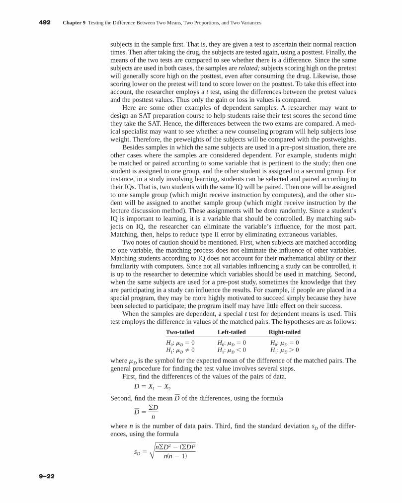
When the samples are dependent, a special t test for dependent means is used. Thistest employs the difference in values of the matched pairs. The hypotheses are as follows:
Two-tailed Left-tailed Right-tailed
H0: mD � 0 H0: mD � 0 H0: mD � 0H1: mD � 0 H1: mD � 0 H1: mD � 0
where mD is the symbol for the expected mean of the difference of the matched pairs. Thegeneral procedure for finding the test value involves several steps.
First, find the differences of the values of the pairs of data.
D � X1 � X2
Second, find the mean of the differences, using the formula
where n is the number of data pairs. Third, find the standard deviation sD of the differ-ences, using the formula
sD �An�D2 � ��D�2
n�n � 1�
D ��Dn
D
blu34978_ch09.qxd 8/13/08 6:06 PM Page 492
Confirming Pages
Section 9–3 Testing the Difference Between Two Means: Dependent Samples 493
9–23
Fourth, find the estimated standard error of the differences, which is
Finally, find the test value, using the formula
The formula in the final step follows the basic format of
where the observed value is the mean of the differences. The expected value mD is zero ifthe hypothesis is mD � 0. The standard error of the difference is the standard deviation ofthe difference, divided by the square root of the sample size. Both populations must benormally or approximately normally distributed. Example 9–6 illustrates the hypothesis-testing procedure in detail.
Test value ��observed value� � �expected value�
standard error
t � D � mD
sD �2n with d.f. � n � 1
sD �sD
2n
sD
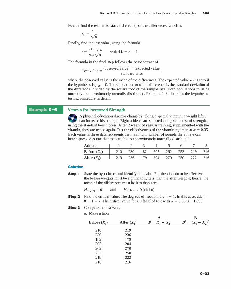
Example 9–6 Vitamin for Increased StrengthA physical education director claims by taking a special vitamin, a weight liftercan increase his strength. Eight athletes are selected and given a test of strength,
using the standard bench press. After 2 weeks of regular training, supplemented with thevitamin, they are tested again. Test the effectiveness of the vitamin regimen at a � 0.05.Each value in these data represents the maximum number of pounds the athlete canbench-press. Assume that the variable is approximately normally distributed.
Athlete 1 2 3 4 5 6 7 8
Before (X1) 210 230 182 205 262 253 219 216
After (X2) 219 236 179 204 270 250 222 216
Solution
Step 1 State the hypotheses and identify the claim. For the vitamin to be effective,the before weights must be significantly less than the after weights; hence, themean of the differences must be less than zero.
H0: mD � 0 and H1: mD � 0 (claim)
Step 2 Find the critical value. The degrees of freedom are n � 1. In this case, d.f. �8 � 1 � 7. The critical value for a left-tailed test with a � 0.05 is �1.895.
Step 3 Compute the test value.
a. Make a table.A B
Before (X1) After (X2) D � X1 � X2 D2 � (X1 � X2)2
210 219230 236182 179205 204262 270253 250219 222216 216
blu34978_ch09.qxd 8/13/08 6:06 PM Page 493
Confirming Pages
494 Chapter 9 Testing the Difference Between Two Means, Two Proportions, and Two Variances
9–24
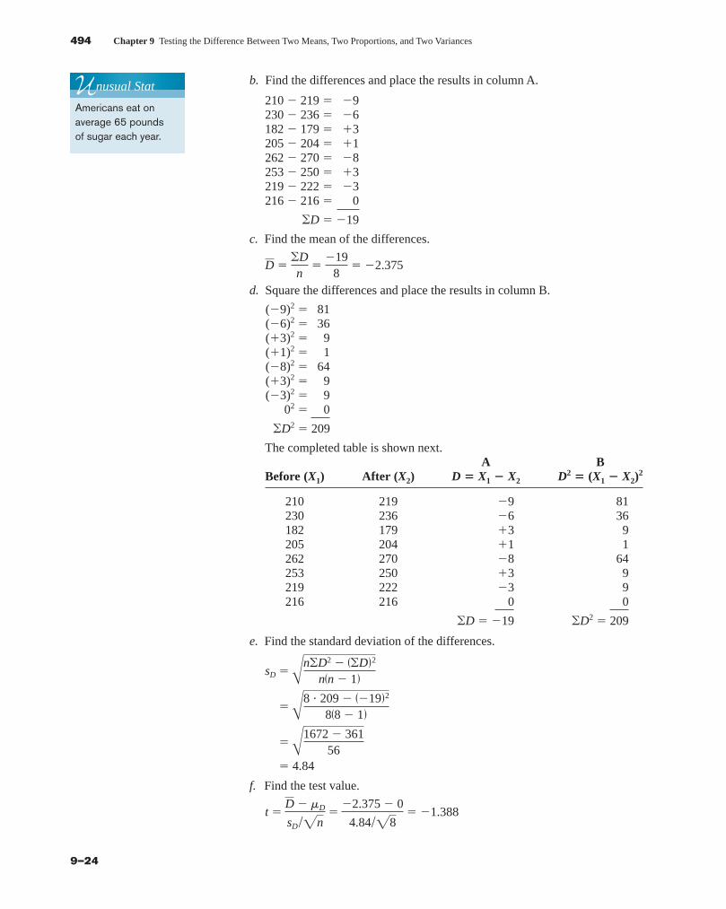
b. Find the differences and place the results in column A.
210 � 219 � �9230 � 236 � �6182 � 179 � �3205 � 204 � �1262 � 270 � �8253 � 250 � �3219 � 222 � �3216 � 216 � 0
�D � �19
c. Find the mean of the differences.
d. Square the differences and place the results in column B.
(�9)2 � 81(�6)2 � 36(�3)2 � 9(�1)2 � 1(�8)2 � 64(�3)2 � 9(�3)2 � 9
02 � 0
�D2 � 209
The completed table is shown next.A B
Before (X1) After (X2) D � X1 � X2 D2 � (X1 � X2)2
210 219 �9 81230 236 �6 36182 179 �3 9205 204 �1 1262 270 �8 64253 250 �3 9219 222 �3 9216 216 0 0
�D � �19 �D2 � 209
e. Find the standard deviation of the differences.
f. Find the test value.
t �D � mD
sD �2n�
�2.375 � 0
4.84�28� �1.388
� 4.84
�A1672 � 361
56
�A8 • 209 � ��19�2
8�8 � 1�
sD �An�D2 � ��D�2
n�n � 1�
D ��Dn
��19
8� �2.375
Unusual Stat
Americans eat onaverage 65 poundsof sugar each year.
blu34978_ch09.qxd 8/13/08 6:06 PM Page 494
Confirming Pages
Section 9–3 Testing the Difference Between Two Means: Dependent Samples 495
9–25
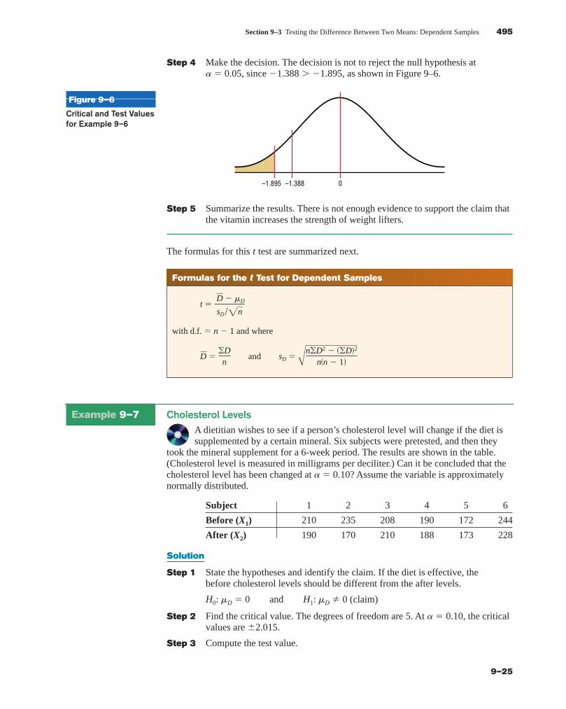
Step 4 Make the decision. The decision is not to reject the null hypothesis at a � 0.05, since �1.388 � �1.895, as shown in Figure 9–6.
Figure 9–6
Critical and Test Valuesfor Example 9–6
0–1.388–1.895
Step 5 Summarize the results. There is not enough evidence to support the claim thatthe vitamin increases the strength of weight lifters.
The formulas for this t test are summarized next.
Formulas for the t Test for Dependent Samples
with d.f. � n � 1 and where
D ��Dn
and sD �An�D2 � ��D�2
n�n � 1�
t � D � mD
sD �2n
Example 9–7 Cholesterol LevelsA dietitian wishes to see if a person’s cholesterol level will change if the diet issupplemented by a certain mineral. Six subjects were pretested, and then they
took the mineral supplement for a 6-week period. The results are shown in the table.(Cholesterol level is measured in milligrams per deciliter.) Can it be concluded that thecholesterol level has been changed at a � 0.10? Assume the variable is approximatelynormally distributed.
Subject 1 2 3 4 5 6
Before (X1) 210 235 208 190 172 244
After (X2) 190 170 210 188 173 228
Solution
Step 1 State the hypotheses and identify the claim. If the diet is effective, the before cholesterol levels should be different from the after levels.
H0: mD � 0 and H1: mD � 0 (claim)
Step 2 Find the critical value. The degrees of freedom are 5. At a � 0.10, the criticalvalues are �2.015.
Step 3 Compute the test value.
blu34978_ch09.qxd 8/13/08 6:06 PM Page 495
Confirming Pages
496 Chapter 9 Testing the Difference Between Two Means, Two Proportions, and Two Variances
9–26
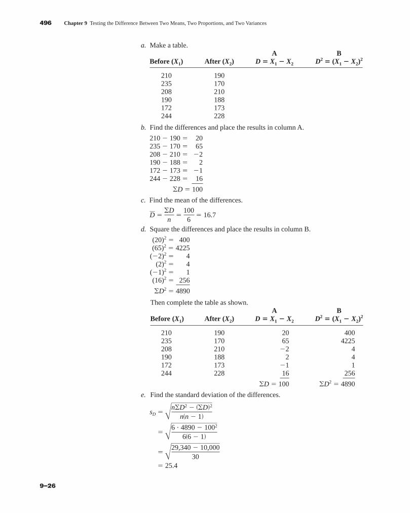
a. Make a table.A B
Before (X1) After (X2) D � X1 � X2 D2 � (X1 � X2)2
210 190235 170208 210190 188172 173244 228
b. Find the differences and place the results in column A.
210 � 190 � 20235 � 170 � 65208 � 210 � �2190 � 188 � 2172 � 173 � �1244 � 228 � 16
�D � 100
c. Find the mean of the differences.
d. Square the differences and place the results in column B.
(20)2 � 400(65)2 � 4225
(�2)2 � 4(2)2 � 4
(�1)2 � 1(16)2 � 256
�D2 � 4890
Then complete the table as shown.A B
Before (X1) After (X2) D � X1 � X2 D2 � (X1 � X2)2
210 190 20 400235 170 65 4225208 210 �2 4190 188 2 4172 173 �1 1244 228 16 256
�D � 100 �D2 � 4890
e. Find the standard deviation of the differences.
� 25.4
�A29,340 � 10,000
30
�A6 • 4890 � 1002
6�6 � 1�
sD �An�D2 � ��D�2
n�n � 1�
D ��Dn
�1006
� 16.7
blu34978_ch09.qxd 8/13/08 6:06 PM Page 496
Confirming Pages
Section 9–3 Testing the Difference Between Two Means: Dependent Samples 497
9–27
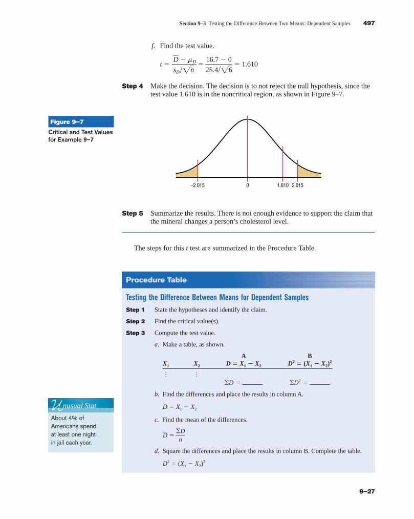
f. Find the test value.
Step 4 Make the decision. The decision is to not reject the null hypothesis, since thetest value 1.610 is in the noncritical region, as shown in Figure 9–7.
t � D � mD
sD �2n�
16.7 � 0
25.4�26� 1.610
Figure 9–7
Critical and Test Valuesfor Example 9–7
0 1.610 2.015–2.015
Step 5 Summarize the results. There is not enough evidence to support the claim thatthe mineral changes a person’s cholesterol level.
The steps for this t test are summarized in the Procedure Table.
Procedure Table
Testing the Difference Between Means for Dependent SamplesStep 1 State the hypotheses and identify the claim.
Step 2 Find the critical value(s).
Step 3 Compute the test value.
a. Make a table, as shown.
A BX1 X2 D � X1 � X2 D2 � (X1 � X2)
2
�D � �D2 �
b. Find the differences and place the results in column A.
D � X1 � X2
c. Find the mean of the differences.
d. Square the differences and place the results in column B. Complete the table.
D2 � (X1 � X2)2
D ��Dn
……
Unusual Stat
About 4% ofAmericans spendat least one night in jail each year.
blu34978_ch09.qxd 8/13/08 6:06 PM Page 497
Confirming Pages
498 Chapter 9 Testing the Difference Between Two Means, Two Proportions, and Two Variances
9–28
The P-values for the t test are found in Table F. For a two-tailed test with d.f. � 5and t � 1.610, the P-value is found between 1.476 and 2.015; hence, 0.10 � P-value �0.20. Thus, the null hypothesis cannot be rejected at a � 0.10.
If a specific difference is hypothesized, this formula should be used
where mD is the hypothesized difference.For example, if a dietitian claims that people on a specific diet will lose an average
of 3 pounds in a week, the hypotheses are
H0: mD � 3 and H1: mD � 3
The value 3 will be substituted in the test statistic formula for mD.Confidence intervals can be found for the mean differences with this formula.
t � D � mD
sD �2n
Procedure Table (continued )
e. Find the standard deviation of the differences.
f. Find the test value.
Step 4 Make the decision.
Step 5 Summarize the results.
t � D � mD
sD �2n with d.f. � n � 1
sD �An �D2 � ��D�2
n�n � 1�
Example 9–8 Find the 90% confidence interval for the data in Example 9–7.
Solution
Substitute in the formula.
Since 0 is contained in the interval, the decision is to not reject the null hypothesis H0: mD � 0.
�4.19 � mD � 37.59 16.7 � 20.89 � mD � 16.7 � 20.89
16.7 � 2.015 •25.4
26� mD � 16.7 � 2.015 •
25.4
26
D � ta2sD
2n� mD � D � ta2
sD
2n
Confidence Interval for the Mean Difference
d.f. � n � 1
D � ta �2sD
2n� mD � D � ta �2
sD
2n
blu34978_ch09.qxd 8/13/08 6:06 PM Page 498
Confirming Pages
Section 9–3 Testing the Difference Between Two Means: Dependent Samples 499
9–29
Applying the Concepts 9–3
Air QualityAs a researcher for the EPA, you have been asked to determine if the air quality in the UnitedStates has changed over the past 2 years. You select a random sample of 10 metropolitan areasand find the number of days each year that the areas failed to meet acceptable air qualitystandards. The data are shown.
Year 1 18 125 9 22 138 29 1 19 17 31
Year 2 24 152 13 21 152 23 6 31 34 20
Source: The World Almanac and Book of Facts.
Based on the data, answer the following questions.
1. What is the purpose of the study?
2. Are the samples independent or dependent?
3. What hypotheses would you use?
4. What is(are) the critical value(s) that you would use?
5. What statistical test would you use?
6. How many degrees of freedom are there?
7. What is your conclusion?
8. Could an independent means test have been used?
9. Do you think this was a good way to answer the original question?
See page 530 for the answers.
Speaking of Statistics
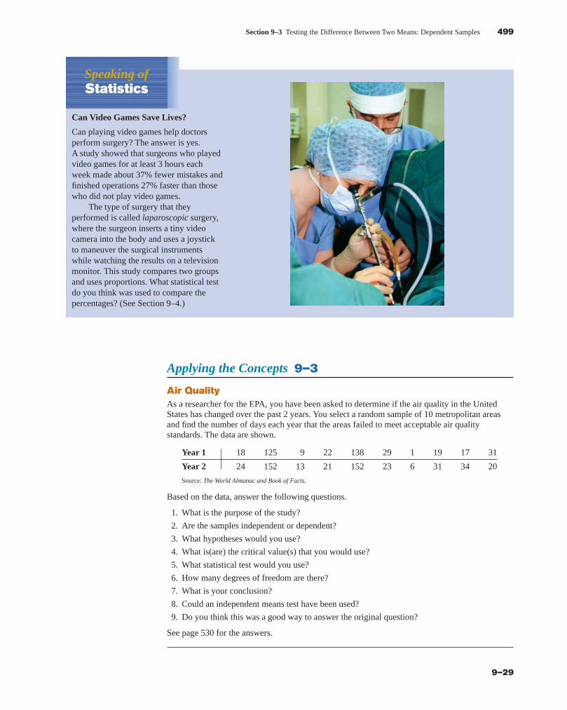
Can Video Games Save Lives?
Can playing video games help doctorsperform surgery? The answer is yes.A study showed that surgeons who playedvideo games for at least 3 hours eachweek made about 37% fewer mistakes andfinished operations 27% faster than thosewho did not play video games.
The type of surgery that theyperformed is called laparoscopic surgery,where the surgeon inserts a tiny videocamera into the body and uses a joystickto maneuver the surgical instrumentswhile watching the results on a televisionmonitor. This study compares two groupsand uses proportions. What statistical testdo you think was used to compare thepercentages? (See Section 9–4.)
blu34978_ch09.qxd 8/13/08 6:06 PM Page 499
Confirming Pages
500 Chapter 9 Testing the Difference Between Two Means, Two Proportions, and Two Variances
9–30
1. Classify each as independent or dependent samples.
a. Heights of identical twinsb. Test scores of the same students in English and
psychologyc. The effectiveness of two different brands of
aspirind. Effects of a drug on reaction time, measured by a
before-and-after teste. The effectiveness of two different diets on two
different groups of individuals
For Exercises 2 through 10, perform each of thesesteps. Assume that all variables are normally orapproximately normally distributed.
a. State the hypotheses and identify the claim.b. Find the critical value(s).c. Compute the test value.d. Make the decision.e. Summarize the results.
Use the traditional method of hypothesis testing unlessotherwise specified.
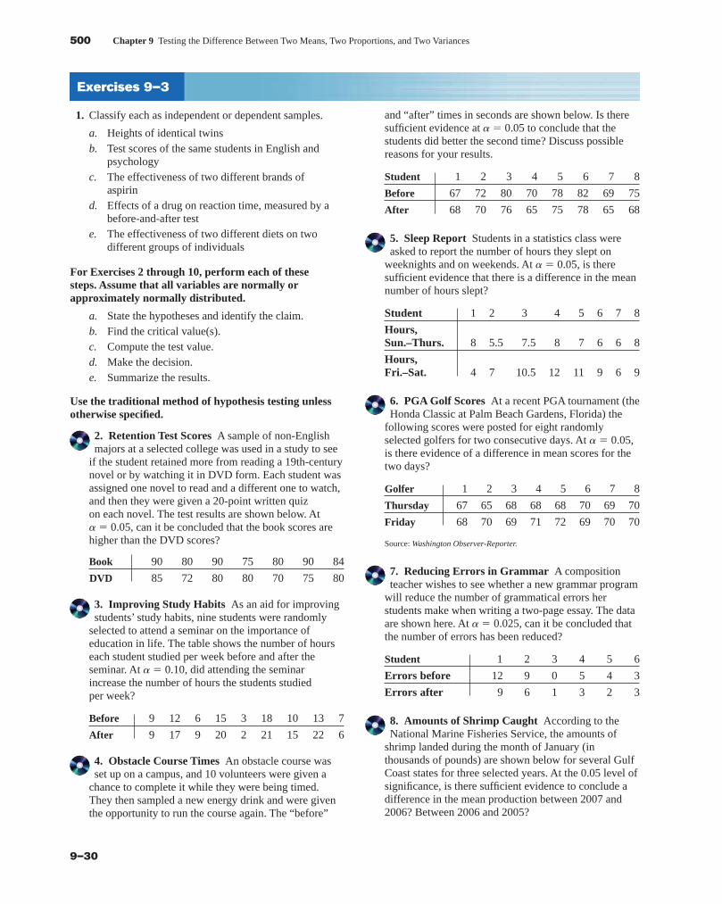
2. Retention Test Scores A sample of non-Englishmajors at a selected college was used in a study to see
if the student retained more from reading a 19th-centurynovel or by watching it in DVD form. Each student wasassigned one novel to read and a different one to watch,and then they were given a 20-point written quizon each novel. The test results are shown below. Ata � 0.05, can it be concluded that the book scores arehigher than the DVD scores?
Book 90 80 90 75 80 90 84
DVD 85 72 80 80 70 75 80
3. Improving Study Habits As an aid for improvingstudents’ study habits, nine students were randomly
selected to attend a seminar on the importance ofeducation in life. The table shows the number of hourseach student studied per week before and after theseminar. At a � 0.10, did attending the seminarincrease the number of hours the students studiedper week?
Before 9 12 6 15 3 18 10 13 7
After 9 17 9 20 2 21 15 22 6
4. Obstacle Course Times An obstacle course wasset up on a campus, and 10 volunteers were given a
chance to complete it while they were being timed.They then sampled a new energy drink and were giventhe opportunity to run the course again. The “before”
and “after” times in seconds are shown below. Is theresufficient evidence at a � 0.05 to conclude that thestudents did better the second time? Discuss possiblereasons for your results.
Student 1 2 3 4 5 6 7 8
Before 67 72 80 70 78 82 69 75
After 68 70 76 65 75 78 65 68
5. Sleep Report Students in a statistics class wereasked to report the number of hours they slept on
weeknights and on weekends. At a � 0.05, is theresufficient evidence that there is a difference in the meannumber of hours slept?
Student 1 2 3 4 5 6 7 8
Hours, Sun.–Thurs. 8 5.5 7.5 8 7 6 6 8
Hours, Fri.–Sat. 4 7 10.5 12 11 9 6 9
6. PGA Golf Scores At a recent PGA tournament (theHonda Classic at Palm Beach Gardens, Florida) the
following scores were posted for eight randomlyselected golfers for two consecutive days. At a � 0.05,is there evidence of a difference in mean scores for thetwo days?
Golfer 1 2 3 4 5 6 7 8
Thursday 67 65 68 68 68 70 69 70
Friday 68 70 69 71 72 69 70 70
Source: Washington Observer-Reporter.
7. Reducing Errors in Grammar A compositionteacher wishes to see whether a new grammar program
will reduce the number of grammatical errors herstudents make when writing a two-page essay. The dataare shown here. At a � 0.025, can it be concluded thatthe number of errors has been reduced?
Student 1 2 3 4 5 6
Errors before 12 9 0 5 4 3
Errors after 9 6 1 3 2 3
8. Amounts of Shrimp Caught According to theNational Marine Fisheries Service, the amounts of
shrimp landed during the month of January (inthousands of pounds) are shown below for several GulfCoast states for three selected years. At the 0.05 level ofsignificance, is there sufficient evidence to conclude adifference in the mean production between 2007 and2006? Between 2006 and 2005?
Exercises 9–3
blu34978_ch09.qxd 8/13/08 6:06 PM Page 500
Confirming Pages

Section 9–3 Testing the Difference Between Two Means: Dependent Samples 501
9–31
Florida Alabama Mississippi Louisiana Texas
2007 344.4 207.0 169.0 1711.5 861.8
2006 1262.0 960.0 529.0 1969.0 1405.0
2005 944.0 541.0 330.0 2300.0 613.0Source: www.st.nmfs.gov
9. Pulse Rates of Identical Twins A researcherwanted to compare the pulse rates of identical twins to
see whether there was any difference. Eight sets of twinswere selected. The rates are given in the table as numberof beats per minute. At a � 0.01, is there a significantdifference in the average pulse rates of twins? Find the
Ward A B C D E F G H I J K L M N O P
1994 184 414 22 99 116 49 24 50 282 25 141 45 12 37 9 17
1999 161 382 22 109 120 52 28 50 297 40 148 56 20 38 9 19
Source: Pittsburgh Tribune-Review.
11. Instead of finding the mean of the differences betweenX1 and X2 by subtracting X1 � X2, you can find it byfinding the means of X1 and X2 and then subtracting the
Extending the Conceptsmeans. Show that these two procedures will yield thesame results.
Test the Difference Between Two Means: Dependent SamplesFor Example 9–6, test the effectiveness of the vitamin regimen. Is there a difference in thestrength of the athletes after the treatment?
1. Enter the data into C1 and C2. Name thecolumns Before and After.
2. Select Stat>Basic Statistics>Paired t.
3. Double-click C1 Before for First sample.
4. Double-click C2 After for Secondsample. The second sample will besubtracted from the first. The differencesare not stored or displayed.
5. Click [Options].
6. Change the Alternative to less than.
7. Click [OK] twice.
Technology Step by Step
MINITABStep by Step
99% confidence interval for the difference of the two.Use the P-value method.
Twin A 87 92 78 83 88 90 84 93
Twin B 83 95 79 83 86 93 80 86
10. Assessed Land Values A reporter hypothesizesthat the average assessed values of land in a large city
have changed during a 5-year period. A random sampleof wards is selected, and the data (in millions of dollars)are shown. At a � 0.05, can it be concluded that theaverage taxable assessed values have changed? Use theP-value method.
blu34978_ch09.qxd 8/13/08 6:06 PM Page 501
Confirming Pages
502 Chapter 9 Testing the Difference Between Two Means, Two Proportions, and Two Variances
9–32
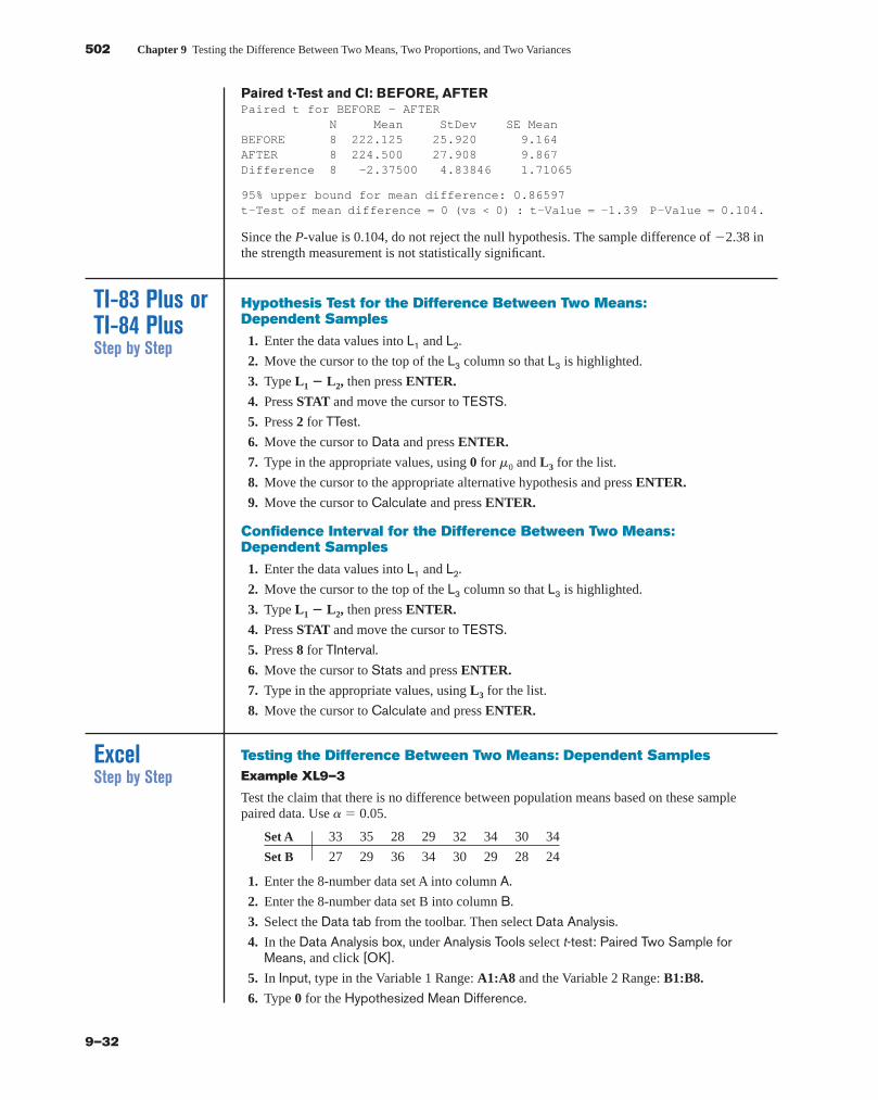
Hypothesis Test for the Difference Between Two Means: Dependent Samples
1. Enter the data values into L1 and L2.2. Move the cursor to the top of the L3 column so that L3 is highlighted.
3. Type L1 � L2, then press ENTER.
4. Press STAT and move the cursor to TESTS.5. Press 2 for TTest.6. Move the cursor to Data and press ENTER.
7. Type in the appropriate values, using 0 for m0 and L3 for the list.
8. Move the cursor to the appropriate alternative hypothesis and press ENTER.
9. Move the cursor to Calculate and press ENTER.
Confidence Interval for the Difference Between Two Means: Dependent Samples
1. Enter the data values into L1 and L2.2. Move the cursor to the top of the L3 column so that L3 is highlighted.
3. Type L1 � L2, then press ENTER.
4. Press STAT and move the cursor to TESTS.5. Press 8 for TInterval.6. Move the cursor to Stats and press ENTER.
7. Type in the appropriate values, using L3 for the list.
8. Move the cursor to Calculate and press ENTER.
TI-83 Plus orTI-84 PlusStep by Step
ExcelStep by Step
Testing the Difference Between Two Means: Dependent SamplesExample XL9–3
Test the claim that there is no difference between population means based on these samplepaired data. Use a� 0.05.
Set A 33 35 28 29 32 34 30 34
Set B 27 29 36 34 30 29 28 24
1. Enter the 8-number data set A into column A.2. Enter the 8-number data set B into column B.3. Select the Data tab from the toolbar. Then select Data Analysis.4. In the Data Analysis box, under Analysis Tools select t-test: Paired Two Sample for
Means, and click [OK].5. In Input, type in the Variable 1 Range: A1:A8 and the Variable 2 Range: B1:B8.
6. Type 0 for the Hypothesized Mean Difference.
Paired t-Test and CI: BEFORE, AFTERPaired t for BEFORE - AFTER
N Mean StDev SE MeanBEFORE 8 222.125 25.920 9.164AFTER 8 224.500 27.908 9.867Difference 8 -2.37500 4.83846 1.71065
95% upper bound for mean difference: 0.86597t-Test of mean difference = 0 (vs < 0) : t-Value = -1.39 P-Value = 0.104.
Since the P-value is 0.104, do not reject the null hypothesis. The sample difference of �2.38 inthe strength measurement is not statistically significant.
blu34978_ch09.qxd 8/13/08 6:06 PM Page 502
Confirming Pages
Section 9–4 Testing the Difference Between Proportions 503
9–33
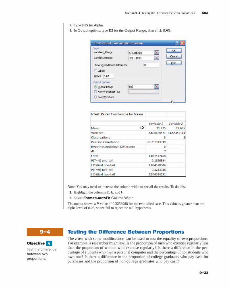
7. Type 0.05 for Alpha.
8. In Output options, type D5 for the Output Range, then click [OK].
Note: You may need to increase the column width to see all the results. To do this:
1. Highlight the columns D, E, and F.
2. Select Format>AutoFit Column Width.
The output shows a P-value of 0.3253988 for the two-tailed case. This value is greater than thealpha level of 0.05, so we fail to reject the null hypothesis.
9–4 Testing the Difference Between ProportionsThe z test with some modifications can be used to test the equality of two proportions.For example, a researcher might ask, Is the proportion of men who exercise regularly lessthan the proportion of women who exercise regularly? Is there a difference in the per-centage of students who own a personal computer and the percentage of nonstudents whoown one? Is there a difference in the proportion of college graduates who pay cash forpurchases and the proportion of non-college graduates who pay cash?
Objective
Test the differencebetween twoproportions.
4
blu34978_ch09.qxd 8/13/08 6:06 PM Page 503
Confirming Pages
504 Chapter 9 Testing the Difference Between Two Means, Two Proportions, and Two Variances
9–34
Recall from Chapter 7 that the symbol (“p hat”) is the sample proportion usedto estimate the population proportion, denoted by p. For example, if in a sample of30 college students, 9 are on probation, then the sample proportion is � , or 0.3. Thepopulation proportion p is the number of all students who are on probation, divided bythe number of students who attend the college. The formula for is
whereX � number of units that possess the characteristic of interestn � sample size
When you are testing the difference between two population proportions p1 and p2, thehypotheses can be stated thus, if no difference between the proportions is hypothesized.
H0: p1 � p2 orH0: p1 � p2 � 0
H1: p1 � p2 H1: p1 � p2 � 0
Similar statements using � or � in the alternate hypothesis can be formed for one-tailedtests.
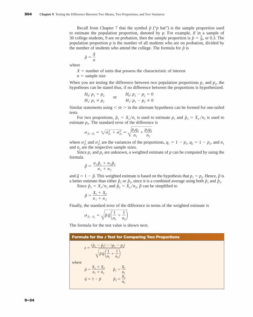
For two proportions, 1 � X1�n1 is used to estimate p1 and 2 � X2 �n2 is used toestimate p2. The standard error of the difference is
where and are the variances of the proportions, q1 � 1 � p1, q2 � 1 � p2, and n1and n2 are the respective sample sizes.
Since p1 and p2 are unknown, a weighted estimate of p can be computed by using theformula
and � 1 � . This weighted estimate is based on the hypothesis that p1 � p2. Hence, isa better estimate than either 1 or 2, since it is a combined average using both 1 and 2.
Since 1 � X1�n1 and 2 � X2�n2, can be simplified to
Finally, the standard error of the difference in terms of the weighted estimate is
The formula for the test value is shown next.
s p̂1� p̂2�A p q ¢ 1
n1�
1n2≤
p �X1 � X2
n 1 � n 2
pp̂p̂p̂p̂p̂p̂ppq
p �n 1 p̂1 � n 2 p̂2
n 1 � n 2
s 2p2
s 2p1
s p̂1�p̂2� 2s2
p1� s2
p2�A
p1q1
n1�
p2q2
n2
p̂p̂
p̂ �Xn
p̂
930p̂
p̂
Formula for the z Test for Comparing Two Proportions
where
q � 1 � p p̂2 �X2
n2
p �X1 � X2
n1 � n2 p̂1 �
X1
n1
z �� p̂1 � p̂2� � �p1 � p2�
A p q ¢ 1n1
�1n2≤
blu34978_ch09.qxd 8/13/08 6:06 PM Page 504
Confirming Pages
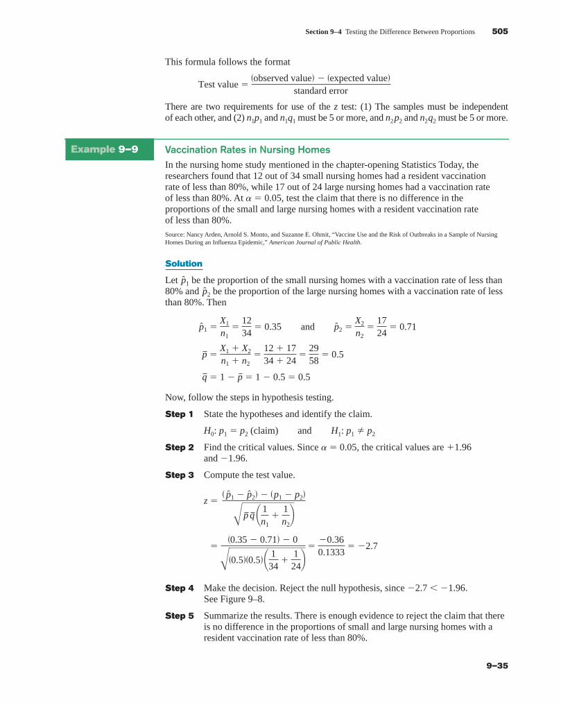
Section 9–4 Testing the Difference Between Proportions 505
9–35
This formula follows the format
There are two requirements for use of the z test: (1) The samples must be independentof each other, and (2) n1p1 and n1q1 must be 5 or more, and n2p2 and n2q2 must be 5 or more.
Test value ��observed value� � �expected value�
standard error
Example 9–9 Vaccination Rates in Nursing HomesIn the nursing home study mentioned in the chapter-opening Statistics Today, theresearchers found that 12 out of 34 small nursing homes had a resident vaccinationrate of less than 80%, while 17 out of 24 large nursing homes had a vaccination rateof less than 80%. At a � 0.05, test the claim that there is no difference in theproportions of the small and large nursing homes with a resident vaccination rateof less than 80%.Source: Nancy Arden, Arnold S. Monto, and Suzanne E. Ohmit, “Vaccine Use and the Risk of Outbreaks in a Sample of NursingHomes During an Influenza Epidemic,” American Journal of Public Health.
Solution
Let 1 be the proportion of the small nursing homes with a vaccination rate of less than80% and 2 be the proportion of the large nursing homes with a vaccination rate of lessthan 80%. Then
Now, follow the steps in hypothesis testing.
Step 1 State the hypotheses and identify the claim.
H0: p1 � p2 (claim) and H1: p1 � p2
Step 2 Find the critical values. Since a � 0.05, the critical values are �1.96and �1.96.
Step 3 Compute the test value.
Step 4 Make the decision. Reject the null hypothesis, since �2.7 � �1.96. See Figure 9–8.
Step 5 Summarize the results. There is enough evidence to reject the claim that thereis no difference in the proportions of small and large nursing homes with aresident vaccination rate of less than 80%.
��0.35 � 0.71� � 0
A�0.5��0.5� ¢ 134
�1
24≤
��0.360.1333
� �2.7
z � � p̂1 � p̂2� � �p1 � p2�
A p q ¢ 1n1
�1n2≤
q � 1 � p � 1 � 0.5 � 0.5
p �X1 � X2
n1 � n2�
12 � 1734 � 24
�2958
� 0.5
p̂1 �X1
n1�
1234
� 0.35 and p̂2 �X2
n2�
1724
� 0.71
p̂p̂
blu34978_ch09.qxd 8/13/08 6:06 PM Page 505
Confirming Pages
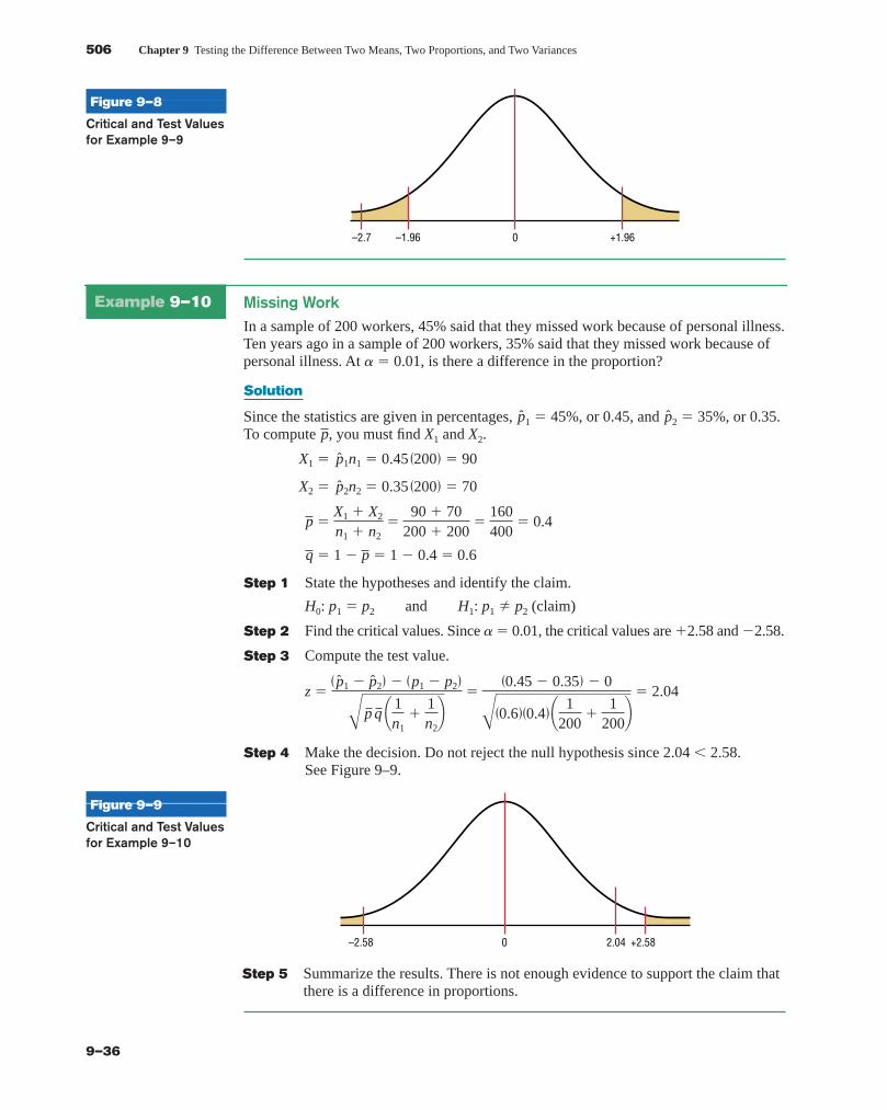
506 Chapter 9 Testing the Difference Between Two Means, Two Proportions, and Two Variances
9–36
0–2.7 +1.96–1.96
Figure 9–8
Critical and Test Valuesfor Example 9–9
Example 9–10 Missing WorkIn a sample of 200 workers, 45% said that they missed work because of personal illness.Ten years ago in a sample of 200 workers, 35% said that they missed work because ofpersonal illness. At a � 0.01, is there a difference in the proportion?
Solution
Since the statistics are given in percentages, 1 � 45%, or 0.45, and 2 � 35%, or 0.35.To compute , you must find X1 and X2.
Step 1 State the hypotheses and identify the claim.
H0: p1 � p2 and H1: p1 � p2 (claim)
Step 2 Find the critical values. Since a� 0.01, the critical values are �2.58 and �2.58.
Step 3 Compute the test value.
Step 4 Make the decision. Do not reject the null hypothesis since 2.04 � 2.58.See Figure 9–9.
��0.45 � 0.35� � 0
A�0.6��0.4� ¢ 1200
�1
200≤
� 2.04z �� p̂1 � p̂2� � �p1 � p2�
A p q ¢ 1n1
�1n2≤
q � 1 � p � 1 � 0.4 � 0.6
p �X1 � X2
n1 � n2�
90 � 70200 � 200
�160400
� 0.4
X2 � p̂2n2 � 0.35 �200� � 70
X1 � p̂1n1 � 0.45 �200� � 90
pp̂p̂
0 +2.58–2.58 2.04
Figure 9–9
Critical and Test Valuesfor Example 9–10
Step 5 Summarize the results. There is not enough evidence to support the claim thatthere is a difference in proportions.
blu34978_ch09.qxd 8/13/08 6:06 PM Page 506
Confirming Pages
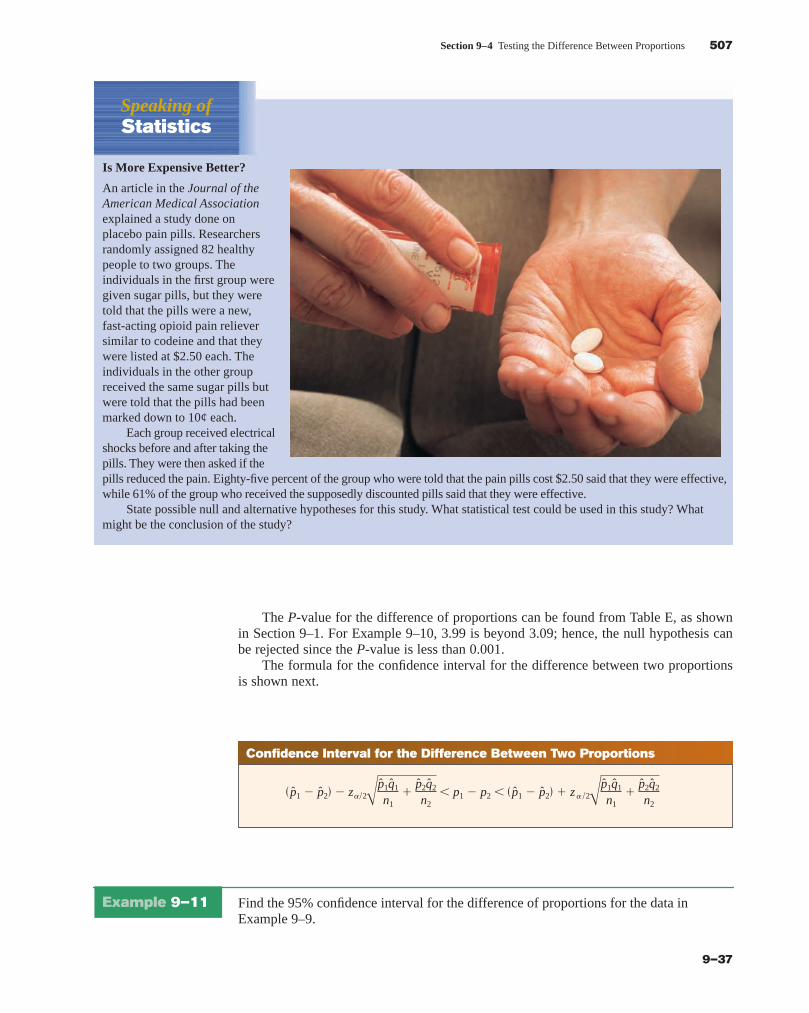
Section 9–4 Testing the Difference Between Proportions 507
9–37
The P-value for the difference of proportions can be found from Table E, as shownin Section 9–1. For Example 9–10, 3.99 is beyond 3.09; hence, the null hypothesis canbe rejected since the P-value is less than 0.001.
The formula for the confidence interval for the difference between two proportionsis shown next.
Speaking of Statistics
Is More Expensive Better?
An article in the Journal of theAmerican Medical Associationexplained a study done onplacebo pain pills. Researchersrandomly assigned 82 healthypeople to two groups. Theindividuals in the first group weregiven sugar pills, but they weretold that the pills were a new,fast-acting opioid pain relieversimilar to codeine and that theywere listed at $2.50 each. Theindividuals in the other groupreceived the same sugar pills butwere told that the pills had beenmarked down to 10¢ each.
Each group received electricalshocks before and after taking thepills. They were then asked if thepills reduced the pain. Eighty-five percent of the group who were told that the pain pills cost $2.50 said that they were effective,while 61% of the group who received the supposedly discounted pills said that they were effective.
State possible null and alternative hypotheses for this study. What statistical test could be used in this study? Whatmight be the conclusion of the study?
Confidence Interval for the Difference Between Two Proportions
� p̂1 � p̂2� � za �2Ap̂1q̂1
n1�
p̂2q̂2
n2� p1 � p2 � � p̂1 � p̂2� � za �2A
p̂1q̂1
n1�
p̂2q̂2
n2
Example 9–11 Find the 95% confidence interval for the difference of proportions for the data inExample 9–9.
blu34978_ch09.qxd 8/13/08 6:06 PM Page 507
Confirming Pages
508 Chapter 9 Testing the Difference Between Two Means, Two Proportions, and Two Variances
9–38
Applying the Concepts 9–4
Smoking and EducationYou are researching the hypothesis that there is no difference in the percent of public schoolstudents who smoke and the percent of private school students who smoke. You find theseresults from a recent survey.
School Percent who smoke
Public 32.3Private 14.5
Based on these figures, answer the following questions.
1. What hypotheses would you use if you wanted to compare percentages of the publicschool students who smoke with the private school students who smoke?
2. What critical value(s) would you use?
3. What statistical test would you use to compare the two percentages?
4. What information would you need to complete the statistical test?
5. Suppose you found that 1000 individuals in each group were surveyed. Could you performthe statistical test?
6. If so, complete the test and summarize the results.
See page 530 for the answers.
Solution
Substitute in the formula.
Since 0 is not contained in the interval, the decision is to reject the null hypothesisH0: p1 � p2.
�0.602 � p1 � p2 � �0.118
�0.36 � 0.242 � p1 � p2 � �0.36 � 0.242
� p1 � p2 � �0.35 � 0.71� � 1.96A�0.35��0.65�
34�
�0.71��0.29�
24
�0.35 � 0.71� � 1.96A�0.35��0.65�
34�
�0.71��0.29�
24
� � p̂1 � p̂2� � za�2Ap̂1q̂1
n1�
p̂2q̂2
n2
� p̂1 � p̂2� � za�2Ap̂1q̂1
n1�
p̂2q̂2
n2� p1 � p2
p̂2 �1724
� 0.71 q̂2 � 0.29
p̂1 �1234
� 0.35 q̂1 � 0.65
blu34978_ch09.qxd 8/13/08 6:06 PM Page 508
Confirming Pages
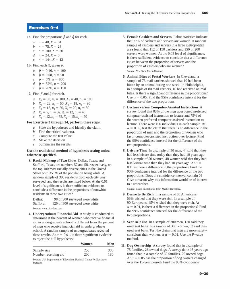
Section 9–4 Testing the Difference Between Proportions 509
9–39
1a. Find the proportions and for each.
a. n � 48, X � 34b. n � 75, X � 28c. n � 100, X � 50d. n � 24, X � 6e. n � 144, X � 12
1b. Find each X, given .
a. � 0.16, n � 100b. � 0.08, n � 50c. � 6%, n � 800d. � 52%, n � 200e. � 20%, n � 150
2. Find and for each.
a. X1 � 60, n1 � 100, X2 � 40, n2 � 100b. X1 � 22, n1 � 50, X2 � 18, n2 � 30c. X1 � 18, n1 � 60, X2 � 20, n2 � 80d. X1 � 5, n1 � 32, X2 � 12, n2 � 48e. X1 � 12, n1 � 75, X2 � 15, n2 � 50
For Exercises 3 through 14, perform these steps.
a. State the hypotheses and identify the claim.b. Find the critical value(s).c. Compute the test value.d. Make the decision.e. Summarize the results.
Use the traditional method of hypothesis testing unlessotherwise specified.
3. Racial Makeup of Two Cities Dallas, Texas, andStafford, Texas, are numbers 57 and 58, respectively, onthe top 100 most racially diverse cities in the UnitedStates with 35.6% of the population being white. Arandom sample of 300 residents from each city wassurveyed, and the results are listed below. At the 0.01level of significance, is there sufficient evidence toconclude a difference in the proportions of nonwhiteresidents in these two cities?
Dallas: 98 of 300 surveyed were whiteStafford: 120 of 300 surveyed were whiteSource: www.city-data.com
4. Undergraduate Financial Aid A study is conducted todetermine if the percent of women who receive financialaid in undergraduate school is different from the percentof men who receive financial aid in undergraduateschool. A random sample of undergraduates revealedthese results. At a� 0.01, is there significant evidenceto reject the null hypothesis?
Women Men
Sample size 250 300Number receiving aid 200 180Source: U.S. Department of Education, National Center for EducationStatistics.
qp
p̂p̂p̂p̂p̂
p̂
q̂p̂ 5. Female Cashiers and Servers Labor statistics indicatethat 77% of cashiers and servers are women. A randomsample of cashiers and servers in a large metropolitanarea found that 112 of 150 cashiers and 150 of 200servers were women. At the 0.05 level of significance,is there sufficient evidence to conclude that a differenceexists between the proportion of servers and theproportion of cashiers who are women?Source: New York Times Almanac.
6. Animal Bites of Postal Workers In Cleveland, asample of 73 mail carriers showed that 10 had beenbitten by an animal during one week. In Philadelphia,in a sample of 80 mail carriers, 16 had received animalbites. Is there a significant difference in the proportions?Use a � 0.05. Find the 95% confidence interval for thedifference of the two proportions.
7. Lecture versus Computer-Assisted Instruction Asurvey found that 83% of the men questioned preferredcomputer-assisted instruction to lecture and 75% ofthe women preferred computer-assisted instruction tolecture. There were 100 individuals in each sample. Ata � 0.05, test the claim that there is no difference in theproportion of men and the proportion of women whofavor computer-assisted instruction over lecture. Findthe 95% confidence interval for the difference of thetwo proportions.
8. Leisure Time In a sample of 50 men, 44 said that theyhad less leisure time today than they had 10 years ago.In a sample of 50 women, 48 women said that they hadless leisure time than they had 10 years ago. At a �0.10 is there a difference in the proportion? Find the90% confidence interval for the difference of the twoproportions. Does the confidence interval contain 0?Give a reason why this information would be of interestto a researcher.Source: Based on statistics from Market Directory.
9. Desire to Be Rich In a sample of 80 Americans, 55% wished that they were rich. In a sample of90 Europeans, 45% wished that they were rich. At a � 0.01, is there a difference in the proportions? Findthe 99% confidence interval for the difference of thetwo proportions.
10. Seat Belt Use In a sample of 200 men, 130 said theyused seat belts. In a sample of 300 women, 63 said theyused seat belts. Test the claim that men are more safety-conscious than women, at a � 0.01. Use the P-valuemethod.
11. Dog Ownership A survey found that in a sample of75 families, 26 owned dogs. A survey done 15 years agofound that in a sample of 60 families, 26 owned dogs.At a � 0.05 has the proportion of dog owners changedover the 15-year period? Find the 95% confidence
Exercises 9–4
blu34978_ch09.qxd 8/13/08 6:06 PM Page 509
Confirming Pages
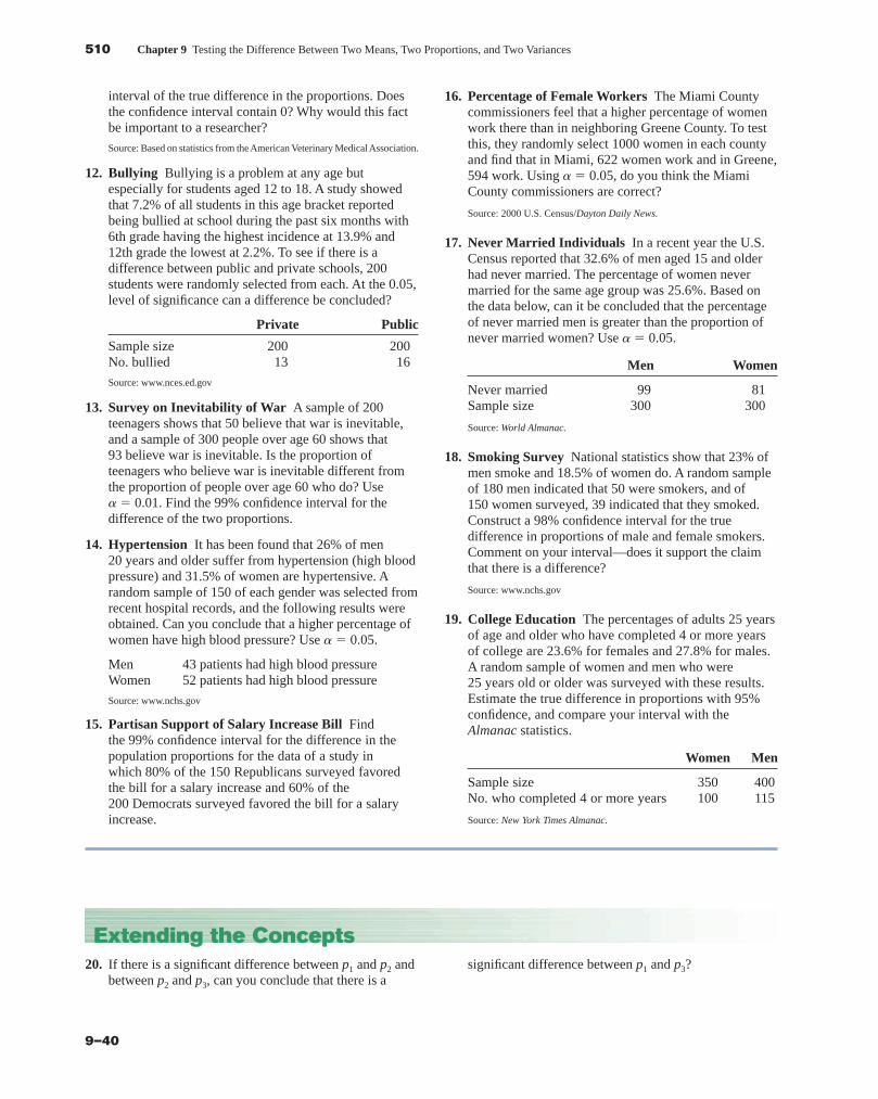
interval of the true difference in the proportions. Doesthe confidence interval contain 0? Why would this factbe important to a researcher?
Source: Based on statistics from the American Veterinary Medical Association.
12. Bullying Bullying is a problem at any age butespecially for students aged 12 to 18. A study showedthat 7.2% of all students in this age bracket reportedbeing bullied at school during the past six months with6th grade having the highest incidence at 13.9% and12th grade the lowest at 2.2%. To see if there is adifference between public and private schools, 200students were randomly selected from each. At the 0.05,level of significance can a difference be concluded?
Private Public
Sample size 200 200No. bullied 13 16
Source: www.nces.ed.gov
13. Survey on Inevitability of War A sample of 200teenagers shows that 50 believe that war is inevitable,and a sample of 300 people over age 60 shows that93 believe war is inevitable. Is the proportion ofteenagers who believe war is inevitable different fromthe proportion of people over age 60 who do? Use a � 0.01. Find the 99% confidence interval for thedifference of the two proportions.
14. Hypertension It has been found that 26% of men20 years and older suffer from hypertension (high bloodpressure) and 31.5% of women are hypertensive. Arandom sample of 150 of each gender was selected fromrecent hospital records, and the following results wereobtained. Can you conclude that a higher percentage ofwomen have high blood pressure? Use a � 0.05.
Men 43 patients had high blood pressureWomen 52 patients had high blood pressure
Source: www.nchs.gov
15. Partisan Support of Salary Increase Bill Findthe 99% confidence interval for the difference in thepopulation proportions for the data of a study inwhich 80% of the 150 Republicans surveyed favoredthe bill for a salary increase and 60% of the200 Democrats surveyed favored the bill for a salaryincrease.
16. Percentage of Female Workers The Miami Countycommissioners feel that a higher percentage of womenwork there than in neighboring Greene County. To testthis, they randomly select 1000 women in each countyand find that in Miami, 622 women work and in Greene,594 work. Using a � 0.05, do you think the MiamiCounty commissioners are correct?
Source: 2000 U.S. Census/Dayton Daily News.
17. Never Married Individuals In a recent year the U.S.Census reported that 32.6% of men aged 15 and olderhad never married. The percentage of women nevermarried for the same age group was 25.6%. Based onthe data below, can it be concluded that the percentageof never married men is greater than the proportion ofnever married women? Use a � 0.05.
Men Women
Never married 99 81Sample size 300 300
Source: World Almanac.
18. Smoking Survey National statistics show that 23% ofmen smoke and 18.5% of women do. A random sampleof 180 men indicated that 50 were smokers, and of150 women surveyed, 39 indicated that they smoked.Construct a 98% confidence interval for the truedifference in proportions of male and female smokers.Comment on your interval—does it support the claimthat there is a difference?
Source: www.nchs.gov
19. College Education The percentages of adults 25 yearsof age and older who have completed 4 or more yearsof college are 23.6% for females and 27.8% for males.A random sample of women and men who were25 years old or older was surveyed with these results.Estimate the true difference in proportions with 95%confidence, and compare your interval with theAlmanac statistics.
Women Men
Sample size 350 400No. who completed 4 or more years 100 115
Source: New York Times Almanac.
510 Chapter 9 Testing the Difference Between Two Means, Two Proportions, and Two Variances
9–40
20. If there is a significant difference between p1 and p2 andbetween p2 and p3, can you conclude that there is a
Extending the Conceptssignificant difference between p1 and p3?
blu34978_ch09.qxd 8/13/08 6:06 PM Page 510
Confirming Pages
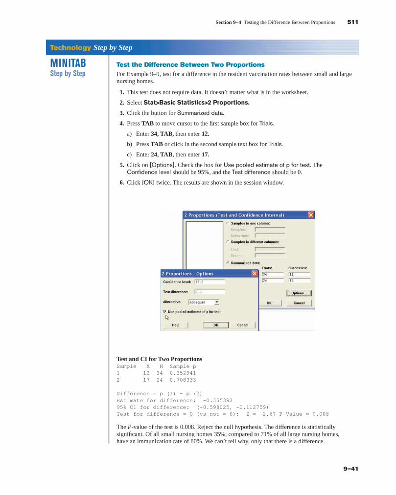
Section 9–4 Testing the Difference Between Proportions 511
9–41
Test the Difference Between Two ProportionsFor Example 9–9, test for a difference in the resident vaccination rates between small and largenursing homes.
1. This test does not require data. It doesn’t matter what is in the worksheet.
2. Select Stat>Basic Statistics>2 Proportions.
3. Click the button for Summarized data.
4. Press TAB to move cursor to the first sample box for Trials.
a) Enter 34, TAB, then enter 12.
b) Press TAB or click in the second sample text box for Trials.
c) Enter 24, TAB, then enter 17.
5. Click on [Options]. Check the box for Use pooled estimate of p for test. TheConfidence level should be 95%, and the Test difference should be 0.
6. Click [OK] twice. The results are shown in the session window.
Test and CI for Two ProportionsSample X N Sample p1 12 34 0.3529412 17 24 0.708333
Difference = p (1) - p (2)Estimate for difference: -0.35539295% CI for difference: (-0.598025, -0.112759)Test for difference = 0 (vs not = 0): Z = -2.67 P-Value = 0.008
The P-value of the test is 0.008. Reject the null hypothesis. The difference is statisticallysignificant. Of all small nursing homes 35%, compared to 71% of all large nursing homes,have an immunization rate of 80%. We can’t tell why, only that there is a difference.
Technology Step by Step
MINITABStep by Step
blu34978_ch09.qxd 8/13/08 6:06 PM Page 511
Confirming Pages
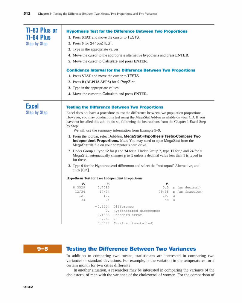
Hypothesis Test for the Difference Between Two Proportions
1. Press STAT and move the cursor to TESTS.
2. Press 6 for 2-PropZTEST.
3. Type in the appropriate values.
4. Move the cursor to the appropriate alternative hypothesis and press ENTER.
5. Move the cursor to Calculate and press ENTER.
Confidence Interval for the Difference Between Two Proportions1. Press STAT and move the cursor to TESTS.
2. Press B (ALPHA APPS) for 2-PropZInt.
3. Type in the appropriate values.
4. Move the cursor to Calculate and press ENTER.
512 Chapter 9 Testing the Difference Between Two Means, Two Proportions, and Two Variances
9–42
TI-83 Plus orTI-84 PlusStep by Step
ExcelStep by Step
Testing the Difference Between Two ProportionsExcel does not have a procedure to test the difference between two population proportions.However, you may conduct this test using the MegaStat Add-in available on your CD. If youhave not installed this add-in, do so, following the instructions from the Chapter 1 Excel Stepby Step.
We will use the summary information from Example 9–9.
1. From the toolbar, select Add-Ins, MegaStat>Hypothesis Tests>Compare TwoIndependent Proportions. Note: You may need to open MegaStat from theMegaStat.xls file on your computer’s hard drive.
2. Under Group 1, type 12 for p and 34 for n. Under Group 2, type 17 for p and 24 for n.MegaStat automatically changes p to X unless a decimal value less than 1 is typed infor these.
3. Type 0 for the Hypothesized difference and select the “not equal” Alternative, andclick [OK].
Hypothesis Test for Two Independent Proportionsp1 p2 pc
0.3529 0.7083 0.5 p (as decimal)12/34 17/24 29/58 p (as fraction)12. 17. 29. X34 24 58 n
�0.3554 Difference0. Hypothesized difference
0.1333 Standard error�2.67 z0.0077 P-value (two-tailed)
9–5 Testing the Difference Between Two VariancesIn addition to comparing two means, statisticians are interested in comparing twovariances or standard deviations. For example, is the variation in the temperatures for acertain month for two cities different?
In another situation, a researcher may be interested in comparing the variance of thecholesterol of men with the variance of the cholesterol of women. For the comparison of
blu34978_ch09.qxd 8/13/08 6:06 PM Page 512
Confirming Pages
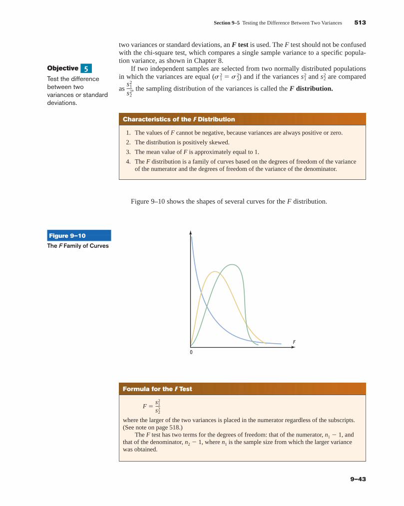
Section 9–5 Testing the Difference Between Two Variances 513
9–43
Characteristics of the F Distribution
1. The values of F cannot be negative, because variances are always positive or zero.
2. The distribution is positively skewed.
3. The mean value of F is approximately equal to 1.
4. The F distribution is a family of curves based on the degrees of freedom of the varianceof the numerator and the degrees of freedom of the variance of the denominator.
Objective
Test the differencebetween twovariances or standarddeviations.
5
Figure 9–10 shows the shapes of several curves for the F distribution.
F
0
Figure 9–10
The F Family of Curves
Formula for the F Test
where the larger of the two variances is placed in the numerator regardless of the subscripts.(See note on page 518.)
The F test has two terms for the degrees of freedom: that of the numerator, n1 � 1, andthat of the denominator, n2 � 1, where n1 is the sample size from which the larger variancewas obtained.
F �s2
1
s22
two variances or standard deviations, an F test is used. The F test should not be confusedwith the chi-square test, which compares a single sample variance to a specific popula-tion variance, as shown in Chapter 8.
If two independent samples are selected from two normally distributed populationsin which the variances are equal ( ) and if the variances and are compared
as , the sampling distribution of the variances is called the F distribution.s1
2
s22
s22s2
1s 21 � s 2
2
blu34978_ch09.qxd 8/13/08 6:06 PM Page 513
Confirming Pages
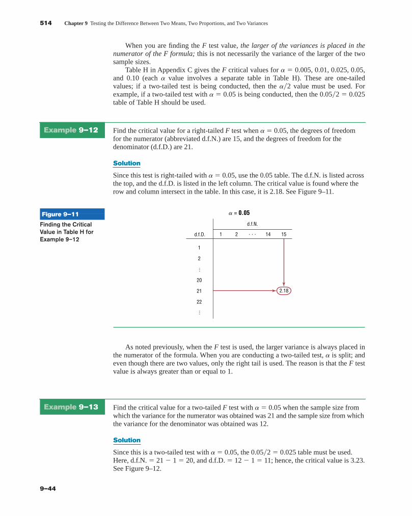
514 Chapter 9 Testing the Difference Between Two Means, Two Proportions, and Two Variances
9–44
When you are finding the F test value, the larger of the variances is placed in thenumerator of the F formula; this is not necessarily the variance of the larger of the twosample sizes.
Table H in Appendix C gives the F critical values for a � 0.005, 0.01, 0.025, 0.05,and 0.10 (each a value involves a separate table in Table H). These are one-tailedvalues; if a two-tailed test is being conducted, then the a�2 value must be used. Forexample, if a two-tailed test with a � 0.05 is being conducted, then the 0.05�2 � 0.025table of Table H should be used.
Example 9–12 Find the critical value for a right-tailed F test when a� 0.05, the degrees of freedomfor the numerator (abbreviated d.f.N.) are 15, and the degrees of freedom for thedenominator (d.f.D.) are 21.
Solution
Since this test is right-tailed with a� 0.05, use the 0.05 table. The d.f.N. is listed acrossthe top, and the d.f.D. is listed in the left column. The critical value is found where therow and column intersect in the table. In this case, it is 2.18. See Figure 9–11.
......
1
1
2
20
21
22
2 . . . 14 15
2.18
d.f.D.
d.f.N.
� = 0.05Figure 9–11
Finding the CriticalValue in Table H forExample 9–12
Example 9–13 Find the critical value for a two-tailed F test with a � 0.05 when the sample size fromwhich the variance for the numerator was obtained was 21 and the sample size from whichthe variance for the denominator was obtained was 12.
Solution
Since this is a two-tailed test with a� 0.05, the 0.05�2 � 0.025 table must be used.Here, d.f.N. � 21 � 1 � 20, and d.f.D. � 12 � 1 � 11; hence, the critical value is 3.23.See Figure 9–12.
As noted previously, when the F test is used, the larger variance is always placed inthe numerator of the formula. When you are conducting a two-tailed test, a is split; andeven though there are two values, only the right tail is used. The reason is that the F testvalue is always greater than or equal to 1.
blu34978_ch09.qxd 8/13/08 6:06 PM Page 514
Confirming Pages
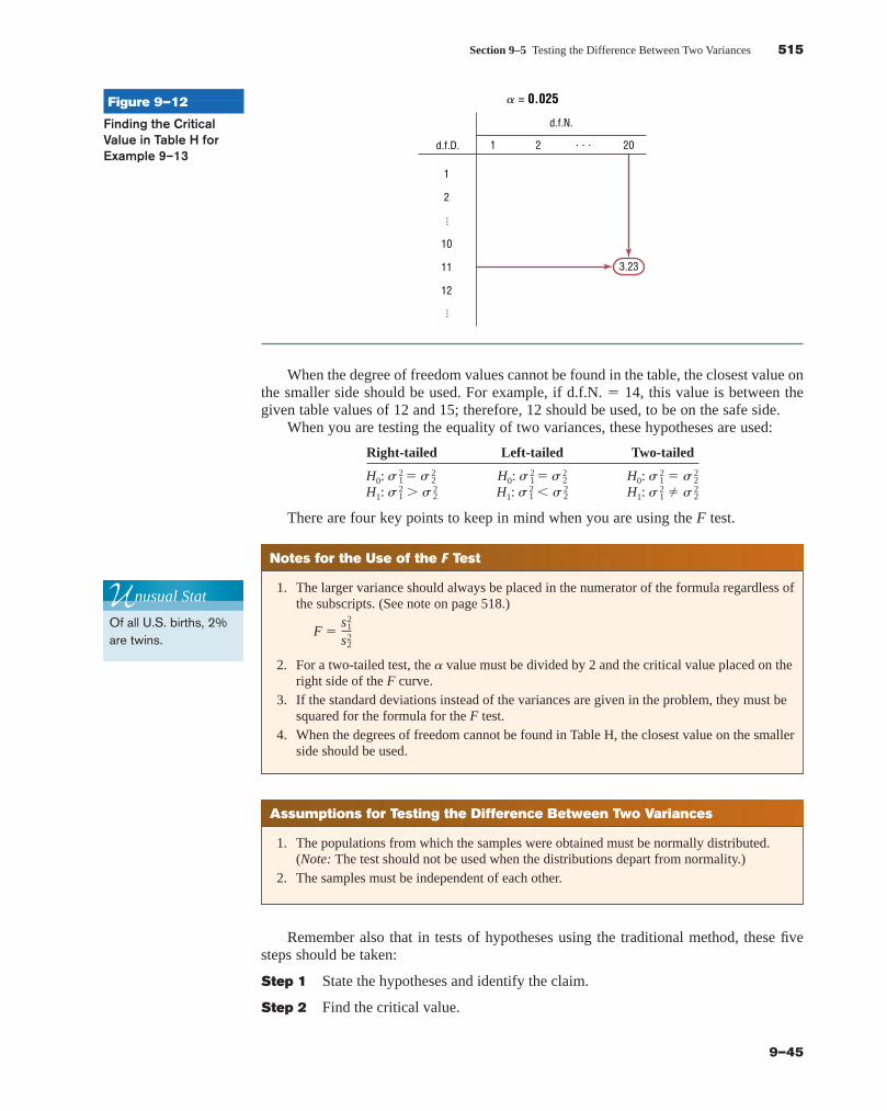
Section 9–5 Testing the Difference Between Two Variances 515
9–45
When the degree of freedom values cannot be found in the table, the closest value onthe smaller side should be used. For example, if d.f.N. � 14, this value is between thegiven table values of 12 and 15; therefore, 12 should be used, to be on the safe side.
When you are testing the equality of two variances, these hypotheses are used:
Right-tailed Left-tailed Two-tailed
H0: H0: H0: H1: H1: H1:
There are four key points to keep in mind when you are using the F test.
s 21 � s 2
2s 21 � s 2
2s 21 � s 2
2
s 21 � s 2
2s 21 � s 2
2s 21 � s 2
2
......
1
1
2
10
11
12
2 . . . 20
3.23
d.f.D.
d.f.N.
� = 0.025Figure 9–12
Finding the CriticalValue in Table H forExample 9–13
Notes for the Use of the F Test
1. The larger variance should always be placed in the numerator of the formula regardless ofthe subscripts. (See note on page 518.)
2. For a two-tailed test, the a value must be divided by 2 and the critical value placed on theright side of the F curve.
3. If the standard deviations instead of the variances are given in the problem, they must besquared for the formula for the F test.
4. When the degrees of freedom cannot be found in Table H, the closest value on the smallerside should be used.
F �s2
1
s22
Assumptions for Testing the Difference Between Two Variances
1. The populations from which the samples were obtained must be normally distributed.(Note: The test should not be used when the distributions depart from normality.)
2. The samples must be independent of each other.
Unusual Stat
Of all U.S. births, 2%are twins.
Remember also that in tests of hypotheses using the traditional method, these fivesteps should be taken:
Step 1 State the hypotheses and identify the claim.
Step 2 Find the critical value.
blu34978_ch09.qxd 8/13/08 6:06 PM Page 515
Confirming Pages
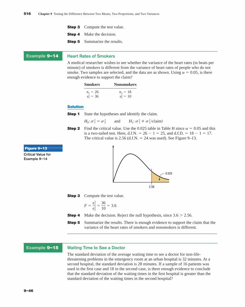
516 Chapter 9 Testing the Difference Between Two Means, Two Proportions, and Two Variances
9–46
Example 9–14 Heart Rates of SmokersA medical researcher wishes to see whether the variance of the heart rates (in beats perminute) of smokers is different from the variance of heart rates of people who do notsmoke. Two samples are selected, and the data are as shown. Using a � 0.05, is thereenough evidence to support the claim?
Smokers Nonsmokers
Solution
Step 1 State the hypotheses and identify the claim.
Step 2 Find the critical value. Use the 0.025 table in Table H since a � 0.05 and thisis a two-tailed test. Here, d.f.N. � 26 � 1 � 25, and d.f.D. � 18 � 1 � 17.The critical value is 2.56 (d.f.N. � 24 was used). See Figure 9–13.
H0: s 21 � s 2
2 and H1: s 21 � s 2
2 �claim�
s22 � 10s2
1 � 36n2 � 18n1 � 26
2.56
0.025
Figure 9–13
Critical Value forExample 9–14
Step 3 Compute the test value.
Step 4 Make the decision. Reject the null hypothesis, since 3.6 � 2.56.
Step 5 Summarize the results. There is enough evidence to support the claim that thevariance of the heart rates of smokers and nonsmokers is different.
F �s2
1
s22
�3610
� 3.6
Step 3 Compute the test value.
Step 4 Make the decision.
Step 5 Summarize the results.
Example 9–15 Waiting Time to See a DoctorThe standard deviation of the average waiting time to see a doctor for non-life-threatening problems in the emergency room at an urban hospital is 32 minutes. At asecond hospital, the standard deviation is 28 minutes. If a sample of 16 patients wasused in the first case and 18 in the second case, is there enough evidence to concludethat the standard deviation of the waiting times in the first hospital is greater than thestandard deviation of the waiting times in the second hospital?
blu34978_ch09.qxd 8/13/08 6:06 PM Page 516
Confirming Pages
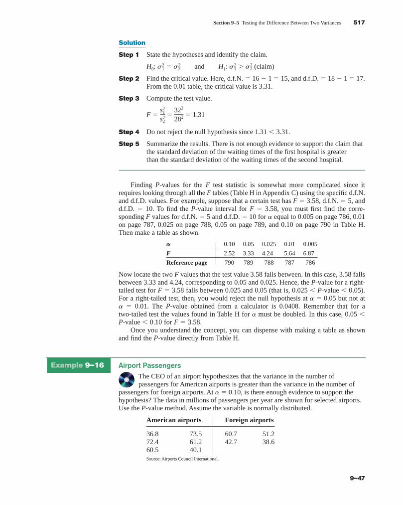
Section 9–5 Testing the Difference Between Two Variances 517
9–47
Example 9–16 Airport PassengersThe CEO of an airport hypothesizes that the variance in the number ofpassengers for American airports is greater than the variance in the number of
passengers for foreign airports. At a � 0.10, is there enough evidence to support thehypothesis? The data in millions of passengers per year are shown for selected airports.Use the P-value method. Assume the variable is normally distributed.
American airports Foreign airports
36.8 73.5 60.7 51.272.4 61.2 42.7 38.660.5 40.1Source: Airports Council International.
Solution
Step 1 State the hypotheses and identify the claim.
H0: � and H1: � (claim)
Step 2 Find the critical value. Here, d.f.N. � 16 � 1 � 15, and d.f.D. � 18 � 1 � 17.From the 0.01 table, the critical value is 3.31.
Step 3 Compute the test value.
Step 4 Do not reject the null hypothesis since 1.31 � 3.31.
Step 5 Summarize the results. There is not enough evidence to support the claim thatthe standard deviation of the waiting times of the first hospital is greaterthan the standard deviation of the waiting times of the second hospital.
Finding P-values for the F test statistic is somewhat more complicated since itrequires looking through all the F tables (Table H in Appendix C) using the specific d.f.N.and d.f.D. values. For example, suppose that a certain test has F � 3.58, d.f.N. � 5, andd.f.D. � 10. To find the P-value interval for F � 3.58, you must first find the corre-sponding F values for d.f.N. � 5 and d.f.D. � 10 for a equal to 0.005 on page 786, 0.01on page 787, 0.025 on page 788, 0.05 on page 789, and 0.10 on page 790 in Table H.Then make a table as shown.
A 0.10 0.05 0.025 0.01 0.005
F 2.52 3.33 4.24 5.64 6.87
Reference page 790 789 788 787 786
Now locate the two F values that the test value 3.58 falls between. In this case, 3.58 fallsbetween 3.33 and 4.24, corresponding to 0.05 and 0.025. Hence, the P-value for a right-tailed test for F � 3.58 falls between 0.025 and 0.05 (that is, 0.025 � P-value � 0.05).For a right-tailed test, then, you would reject the null hypothesis at a � 0.05 but not ata � 0.01. The P-value obtained from a calculator is 0.0408. Remember that for atwo-tailed test the values found in Table H for a must be doubled. In this case, 0.05 �P-value � 0.10 for F � 3.58.
Once you understand the concept, you can dispense with making a table as shownand find the P-value directly from Table H.
F �s2
1
s22
�322
282 � 1.31
s22s2
1s22s2
1
blu34978_ch09.qxd 8/13/08 6:06 PM Page 517
Confirming Pages
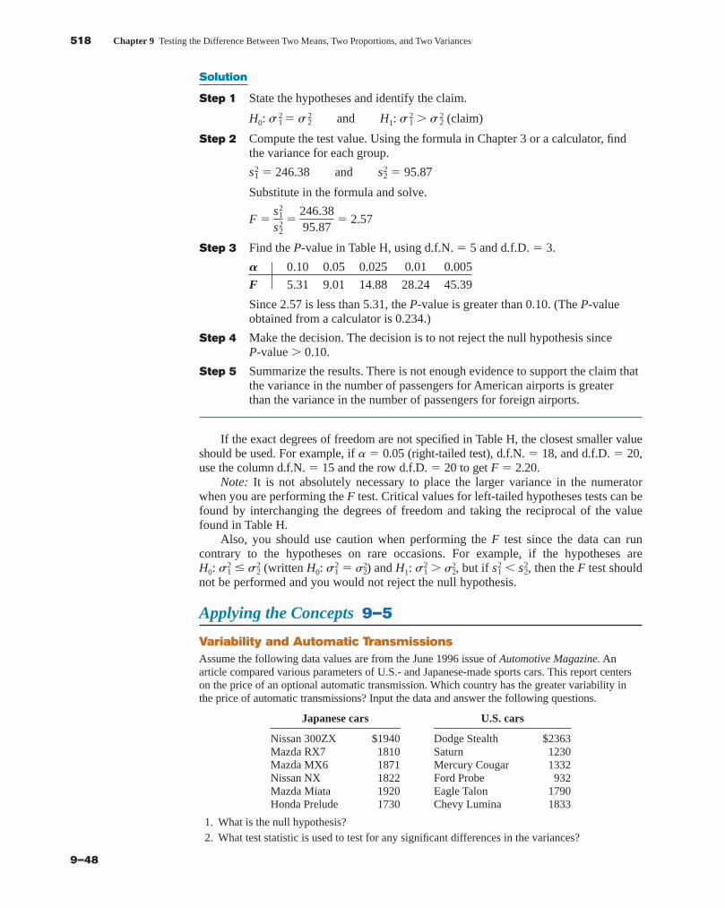
518 Chapter 9 Testing the Difference Between Two Means, Two Proportions, and Two Variances
9–48
Solution
Step 1 State the hypotheses and identify the claim.
H0: and H1: (claim)
Step 2 Compute the test value. Using the formula in Chapter 3 or a calculator, findthe variance for each group.
Substitute in the formula and solve.
Step 3 Find the P-value in Table H, using d.f.N. � 5 and d.f.D. � 3.
A 0.10 0.05 0.025 0.01 0.005
F 5.31 9.01 14.88 28.24 45.39
Since 2.57 is less than 5.31, the P-value is greater than 0.10. (The P-valueobtained from a calculator is 0.234.)
Step 4 Make the decision. The decision is to not reject the null hypothesis sinceP-value � 0.10.
Step 5 Summarize the results. There is not enough evidence to support the claim thatthe variance in the number of passengers for American airports is greaterthan the variance in the number of passengers for foreign airports.
If the exact degrees of freedom are not specified in Table H, the closest smaller valueshould be used. For example, if a � 0.05 (right-tailed test), d.f.N. � 18, and d.f.D. � 20,use the column d.f.N. � 15 and the row d.f.D. � 20 to get F � 2.20.
Note: It is not absolutely necessary to place the larger variance in the numeratorwhen you are performing the F test. Critical values for left-tailed hypotheses tests can befound by interchanging the degrees of freedom and taking the reciprocal of the valuefound in Table H.
Also, you should use caution when performing the F test since the data can runcontrary to the hypotheses on rare occasions. For example, if the hypotheses are H0: � (written H0: � ) and H1: � , but if � , then the F test shouldnot be performed and you would not reject the null hypothesis.
Applying the Concepts 9–5
Variability and Automatic TransmissionsAssume the following data values are from the June 1996 issue of Automotive Magazine. Anarticle compared various parameters of U.S.- and Japanese-made sports cars. This report centerson the price of an optional automatic transmission. Which country has the greater variability inthe price of automatic transmissions? Input the data and answer the following questions.
Japanese cars U.S. cars
Nissan 300ZX $1940 Dodge Stealth $2363Mazda RX7 1810 Saturn 1230Mazda MX6 1871 Mercury Cougar 1332Nissan NX 1822 Ford Probe 932Mazda Miata 1920 Eagle Talon 1790Honda Prelude 1730 Chevy Lumina 1833
1. What is the null hypothesis?2. What test statistic is used to test for any significant differences in the variances?
s22s2
1s22s2
1s22s2
1s22s2
1
F �s2
1
s22
�246.3895.87
� 2.57
s12 � 246.38 and s2
2 � 95.87
s 21 � s 2
2s 21 � s 2
2
blu34978_ch09.qxd 8/13/08 6:06 PM Page 518
Confirming Pages
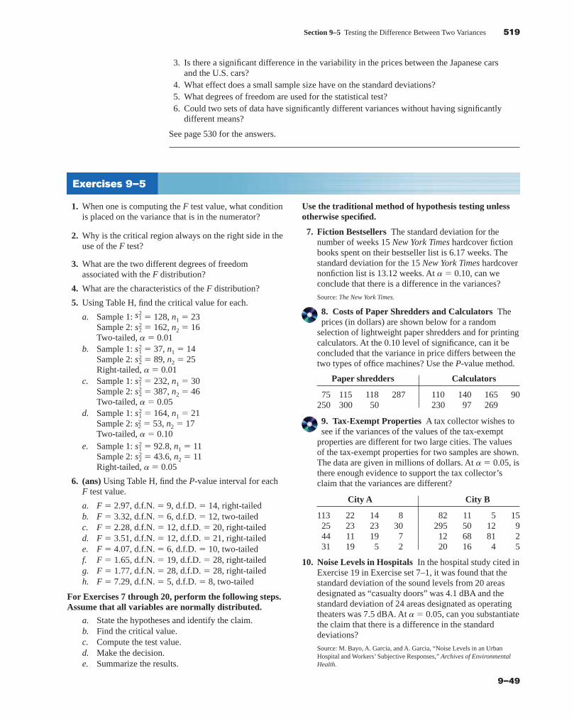
Section 9–5 Testing the Difference Between Two Variances 519
9–49
1. When one is computing the F test value, what conditionis placed on the variance that is in the numerator?
2. Why is the critical region always on the right side in theuse of the F test?
3. What are the two different degrees of freedomassociated with the F distribution?
4. What are the characteristics of the F distribution?
5. Using Table H, find the critical value for each.
a. Sample 1: � 128, n1 � 23Sample 2: � 162, n2 � 16Two-tailed, a � 0.01
b. Sample 1: � 37, n1 � 14Sample 2: � 89, n2 � 25Right-tailed, a � 0.01
c. Sample 1: � 232, n1 � 30Sample 2: � 387, n2 � 46Two-tailed, a � 0.05
d. Sample 1: � 164, n1 � 21Sample 2: � 53, n2 � 17Two-tailed, a � 0.10
e. Sample 1: � 92.8, n1 � 11Sample 2: � 43.6, n2 � 11Right-tailed, a � 0.05
6. (ans) Using Table H, find the P-value interval for eachF test value.
a. F � 2.97, d.f.N. � 9, d.f.D. � 14, right-tailedb. F � 3.32, d.f.N. � 6, d.f.D. � 12, two-tailedc. F � 2.28, d.f.N. � 12, d.f.D. � 20, right-tailedd. F � 3.51, d.f.N. � 12, d.f.D. � 21, right-tailede. F � 4.07, d.f.N. � 6, d.f.D. � 10, two-tailedf. F � 1.65, d.f.N. � 19, d.f.D. � 28, right-tailedg. F � 1.77, d.f.N. � 28, d.f.D. � 28, right-tailedh. F � 7.29, d.f.N. � 5, d.f.D. � 8, two-tailed
For Exercises 7 through 20, perform the following steps.Assume that all variables are normally distributed.
a. State the hypotheses and identify the claim.b. Find the critical value.c. Compute the test value.d. Make the decision.e. Summarize the results.
s22
s21
s22
s21
s22
s21
s22
s21
s22
s21
Use the traditional method of hypothesis testing unlessotherwise specified.
7. Fiction Bestsellers The standard deviation for thenumber of weeks 15 New York Times hardcover fictionbooks spent on their bestseller list is 6.17 weeks. Thestandard deviation for the 15 New York Times hardcovernonfiction list is 13.12 weeks. At a � 0.10, can weconclude that there is a difference in the variances?
Source: The New York Times.
8. Costs of Paper Shredders and Calculators Theprices (in dollars) are shown below for a random
selection of lightweight paper shredders and for printingcalculators. At the 0.10 level of significance, can it beconcluded that the variance in price differs between thetwo types of office machines? Use the P-value method.
Paper shredders Calculators
75 115 118 287 110 140 165 90250 300 50 230 97 269
9. Tax-Exempt Properties A tax collector wishes tosee if the variances of the values of the tax-exempt
properties are different for two large cities. The valuesof the tax-exempt properties for two samples are shown.The data are given in millions of dollars. At a � 0.05, isthere enough evidence to support the tax collector’sclaim that the variances are different?
City A City B
113 22 14 8 82 11 5 1525 23 23 30 295 50 12 944 11 19 7 12 68 81 231 19 5 2 20 16 4 5
10. Noise Levels in Hospitals In the hospital study cited inExercise 19 in Exercise set 7–1, it was found that thestandard deviation of the sound levels from 20 areasdesignated as “casualty doors” was 4.1 dBA and thestandard deviation of 24 areas designated as operatingtheaters was 7.5 dBA. At a� 0.05, can you substantiatethe claim that there is a difference in the standarddeviations?
Source: M. Bayo, A. Garcia, and A. Garcia, “Noise Levels in an UrbanHospital and Workers’ Subjective Responses,” Archives of EnvironmentalHealth.
Exercises 9–5
3. Is there a significant difference in the variability in the prices between the Japanese carsand the U.S. cars?
4. What effect does a small sample size have on the standard deviations?5. What degrees of freedom are used for the statistical test?6. Could two sets of data have significantly different variances without having significantly
different means?
See page 530 for the answers.
blu34978_ch09.qxd 8/13/08 6:06 PM Page 519
Confirming Pages
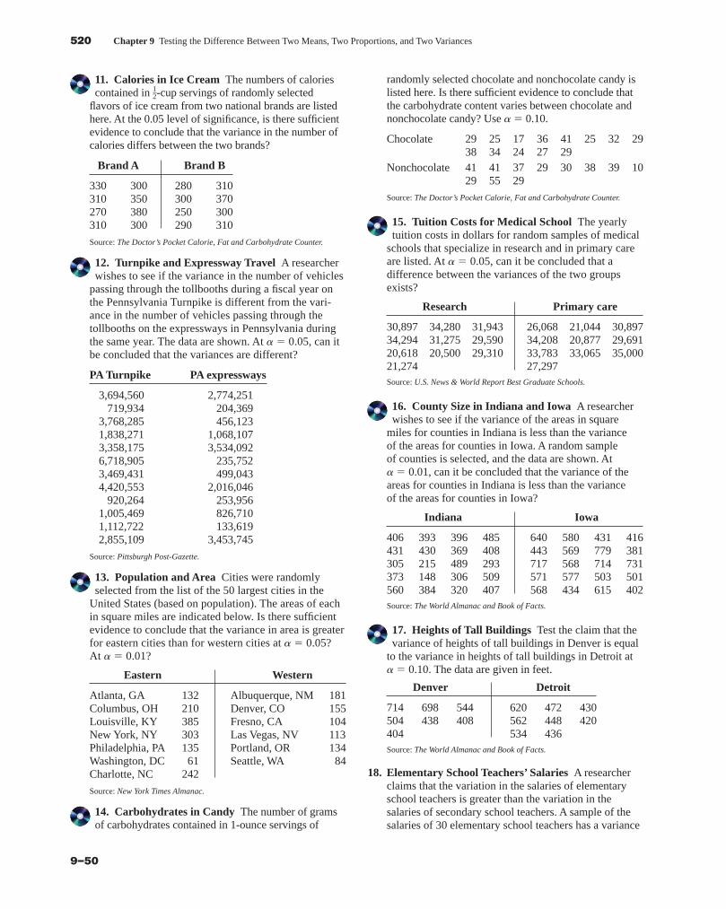
520 Chapter 9 Testing the Difference Between Two Means, Two Proportions, and Two Variances
9–50
11. Calories in Ice Cream The numbers of caloriescontained in -cup servings of randomly selected
flavors of ice cream from two national brands are listedhere. At the 0.05 level of significance, is there sufficientevidence to conclude that the variance in the number ofcalories differs between the two brands?
Brand A Brand B
330 300 280 310310 350 300 370270 380 250 300310 300 290 310
Source: The Doctor’s Pocket Calorie, Fat and Carbohydrate Counter.
12. Turnpike and Expressway Travel A researcherwishes to see if the variance in the number of vehicles
passing through the tollbooths during a fiscal year onthe Pennsylvania Turnpike is different from the vari-ance in the number of vehicles passing through thetollbooths on the expressways in Pennsylvania duringthe same year. The data are shown. At a � 0.05, can itbe concluded that the variances are different?
PA Turnpike PA expressways
3,694,560 2,774,251719,934 204,369
3,768,285 456,1231,838,271 1,068,1073,358,175 3,534,0926,718,905 235,7523,469,431 499,0434,420,553 2,016,046
920,264 253,9561,005,469 826,7101,112,722 133,6192,855,109 3,453,745
Source: Pittsburgh Post-Gazette.
13. Population and Area Cities were randomlyselected from the list of the 50 largest cities in the
United States (based on population). The areas of eachin square miles are indicated below. Is there sufficientevidence to conclude that the variance in area is greaterfor eastern cities than for western cities at a � 0.05? At a � 0.01?
Eastern Western
Atlanta, GA 132 Albuquerque, NM 181Columbus, OH 210 Denver, CO 155Louisville, KY 385 Fresno, CA 104New York, NY 303 Las Vegas, NV 113Philadelphia, PA 135 Portland, OR 134Washington, DC 61 Seattle, WA 84Charlotte, NC 242
Source: New York Times Almanac.
14. Carbohydrates in Candy The number of gramsof carbohydrates contained in 1-ounce servings of
12
randomly selected chocolate and nonchocolate candy islisted here. Is there sufficient evidence to conclude thatthe carbohydrate content varies between chocolate andnonchocolate candy? Use a� 0.10.
Chocolate 29 25 17 36 41 25 32 2938 34 24 27 29
Nonchocolate 41 41 37 29 30 38 39 1029 55 29
Source: The Doctor’s Pocket Calorie, Fat and Carbohydrate Counter.
15. Tuition Costs for Medical School The yearlytuition costs in dollars for random samples of medical
schools that specialize in research and in primary careare listed. At a � 0.05, can it be concluded that adifference between the variances of the two groupsexists?
Research Primary care
30,897 34,280 31,943 26,068 21,044 30,89734,294 31,275 29,590 34,208 20,877 29,69120,618 20,500 29,310 33,783 33,065 35,00021,274 27,297Source: U.S. News & World Report Best Graduate Schools.
16. County Size in Indiana and Iowa A researcherwishes to see if the variance of the areas in square
miles for counties in Indiana is less than the varianceof the areas for counties in Iowa. A random sampleof counties is selected, and the data are shown. Ata � 0.01, can it be concluded that the variance of theareas for counties in Indiana is less than the varianceof the areas for counties in Iowa?
Indiana Iowa
406 393 396 485 640 580 431 416431 430 369 408 443 569 779 381305 215 489 293 717 568 714 731373 148 306 509 571 577 503 501560 384 320 407 568 434 615 402Source: The World Almanac and Book of Facts.
17. Heights of Tall Buildings Test the claim that thevariance of heights of tall buildings in Denver is equal
to the variance in heights of tall buildings in Detroit ata � 0.10. The data are given in feet.
Denver Detroit
714 698 544 620 472 430504 438 408 562 448 420404 534 436Source: The World Almanac and Book of Facts.
18. Elementary School Teachers’ Salaries A researcherclaims that the variation in the salaries of elementaryschool teachers is greater than the variation in thesalaries of secondary school teachers. A sample of thesalaries of 30 elementary school teachers has a variance
blu34978_ch09.qxd 8/13/08 6:06 PM Page 520
Confirming Pages
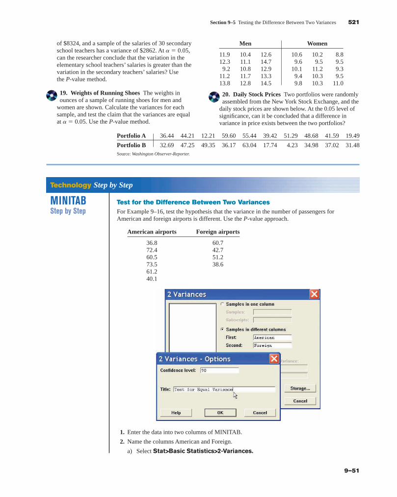
Section 9–5 Testing the Difference Between Two Variances 521
9–51
of $8324, and a sample of the salaries of 30 secondaryschool teachers has a variance of $2862. At a � 0.05,can the researcher conclude that the variation in theelementary school teachers’ salaries is greater than thevariation in the secondary teachers’ salaries? Usethe P-value method.
19. Weights of Running Shoes The weights inounces of a sample of running shoes for men and
women are shown. Calculate the variances for eachsample, and test the claim that the variances are equalat a � 0.05. Use the P-value method.
Men Women
11.9 10.4 12.6 10.6 10.2 8.812.3 11.1 14.7 9.6 9.5 9.59.2 10.8 12.9 10.1 11.2 9.3
11.2 11.7 13.3 9.4 10.3 9.513.8 12.8 14.5 9.8 10.3 11.0
20. Daily Stock Prices Two portfolios were randomlyassembled from the New York Stock Exchange, and the
daily stock prices are shown below. At the 0.05 level ofsignificance, can it be concluded that a difference invariance in price exists between the two portfolios?
Test for the Difference Between Two VariancesFor Example 9–16, test the hypothesis that the variance in the number of passengers forAmerican and foreign airports is different. Use the P-value approach.
American airports Foreign airports
36.8 60.772.4 42.760.5 51.273.5 38.661.240.1
1. Enter the data into two columns of MINITAB.
2. Name the columns American and Foreign.
a) Select Stat>Basic Statistics>2-Variances.
Technology Step by Step
MINITABStep by Step
Portfolio A 36.44 44.21 12.21 59.60 55.44 39.42 51.29 48.68 41.59 19.49
Portfolio B 32.69 47.25 49.35 36.17 63.04 17.74 4.23 34.98 37.02 31.48Source: Washington Observer-Reporter.
blu34978_ch09.qxd 8/13/08 6:06 PM Page 521
Confirming Pages
522 Chapter 9 Testing the Difference Between Two Means, Two Proportions, and Two Variances
9–52
b) Click the button for Samples in different columns.
c) Click in the text box for First, then double-click C1 American.
d) Double-click C2 Foreign, then click on [Options]. The dialog box is shown. Changethe confidence level to 90 and type an appropriate title. In this dialog, we cannotspecify a left- or right-tailed test.
3. Click [OK] twice. A graph window will open that includes a small window that saysF � 2.57 and the P-value is 0.437. Divide this two-tailed P-value by 2 for a one-tailed test.
There is not enough evidence in the sample to conclude there is greater variance in the numberof passengers in American airports compared to foreign airports.
TI-83 Plus orTI-84 Plus Step by Step
Hypothesis Test for the Difference Between Two Variances (Data)
1. Enter the data values into L1 and L2.2. Press STAT and move the cursor to TESTS.3. Press D (ALPHA X�1) for 2-SampFTest. (The TI-84 uses E)
4. Move the cursor to Data and press ENTER.
5. Type in the appropriate values.
6. Move the cursor to the appropriate alternative hypothesis and press ENTER.
7. Move the cursor to Calculate and press ENTER.
Hypothesis Test for the Difference Between Two Variances (Statistics)
1. Press STAT and move the cursor to TESTS.2. Press D (ALPHA X�1) for 2-SampFTest. (The TI-84 uses E)
3. Move the cursor to Stats and press ENTER.
4. Type in the appropriate values.
5. Move the cursor to the appropriate alternative hypothesis and press ENTER.
6. Move the cursor to Calculate and press ENTER.
ExcelStep by Step
F Test for the Difference Between Two VariancesExcel has a two-sample F test included in the Data Analysis Add-in. To perform an F testfor the difference between the variances of two populations, given two independent samples,do this:
1. Enter the first sample data set into column A.
2. Enter the second sample data set into column B.
3. Select the Data tab from the toolbar. Then select Data Analysis.
4. In the Analysis Tools box, select F-test: Two-sample for Variances.
5. Type the ranges for the data in columns A and B.
6. Specify the confidence level Alpha.
7. Specify a location for the output, and click [OK].
Example XL9–4
At a � 0.05, test the hypothesis that the two population variances are equal, using thesample data provided here.
Set A 63 73 80 60 86 83 70 72 82
Set B 86 93 64 82 81 75 88 63 63
blu34978_ch09.qxd 8/13/08 6:06 PM Page 522
Confirming Pages
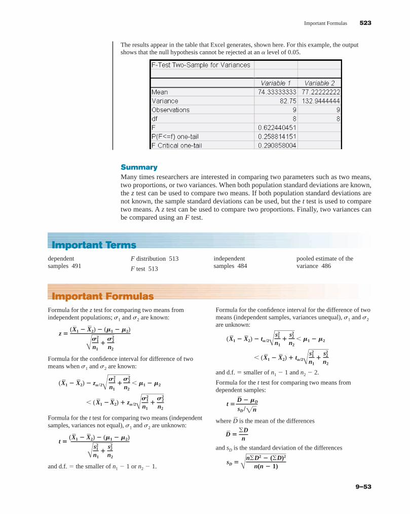
Important Formulas 523
9–53
independent samples 484
pooled estimate of thevariance 486
dependent samples 491
F distribution 513
F test 513
Important Terms
Formula for the z test for comparing two means fromindependent populations; s1 and s2 are known:
Formula for the confidence interval for difference of twomeans when s1 and s2 are known:
Formula for the t test for comparing two means (independentsamples, variances not equal), s1 and s2 are unknown:
and d.f. � the smaller of n1 � 1 or n2 � 1.
t �(X1 � X2) � (M1 � M2)
As2
1
n1�
s22
n2
� (X1 � X2) � zA /2AS2
1
n1�S2
2
n2
(X1 � X2) � zA /2AS2
1
n1�S2
2
n2� M1 � M2
z �( X1 � X2) � (M1 � M2)
AS2
1
n1�S2
2
n2
Formula for the confidence interval for the difference of twomeans (independent samples, variances unequal), s1 and s2
are unknown:
and d.f. � smaller of n1 � 1 and n2 � 2.
Formula for the t test for comparing two means fromdependent samples:
where is the mean of the differences
and sD is the standard deviation of the differences
sD �An�D2 � (�D)2
n(n � 1)
D ��Dn
D
t � D � MD
sD /2n
� (X1 � X2) � tA/2As2
1
n1�
s22
n2
(X1 � X2) � tA /2As2
1
n1�
s22
n2� M1 � M2
Important Formulas
The results appear in the table that Excel generates, shown here. For this example, the outputshows that the null hypothesis cannot be rejected at an a level of 0.05.
SummaryMany times researchers are interested in comparing two parameters such as two means,two proportions, or two variances. When both population standard deviations are known,the z test can be used to compare two means. If both population standard deviations arenot known, the sample standard deviations can be used, but the t test is used to comparetwo means. A z test can be used to compare two proportions. Finally, two variances canbe compared using an F test.
blu34978_ch09.qxd 8/13/08 6:06 PM Page 523
Confirming Pages
524 Chapter 9 Testing the Difference Between Two Means, Two Proportions, and Two Variances
9–54
Review ExercisesFor each exercise, perform these steps. Assume that allvariables are normally or approximately normallydistributed.
a. State the hypotheses and identify the claim.b. Find the critical value(s).c. Compute the test value.d. Make the decision.e. Summarize the results.
Use the traditional method of hypothesis testing unlessotherwise specified.
1. Driving for Pleasure Two groups of drivers aresurveyed to see how many miles per week they drive
for pleasure trips. The data are shown. At a � 0.01, canit be concluded that single drivers do more driving forpleasure trips on average than married drivers? Assumes1 � 16.7 and s2 � 16.1.
Single drivers Married drivers
106 110 115 121 132 97 104 138 102 115119 97 118 122 135 133 120 119 136 96110 117 116 138 142 139 108 117 145 114115 114 103 98 99 140 136 113 113 150108 117 152 147 117 101 114 116 113 135154 86 115 116 104 115 109 147 106 88107 133 138 142 140 113 119 99 108 105
2. Average Earnings of College Graduates The averageyearly earnings of male college graduates (with atleast a bachelor’s degree) are $58,500 for men aged25 to 34. The average yearly earnings of female college
graduates with the same qualifications are $49,339.Based on the results below, can it be concluded thatthere is a difference in mean earnings between maleand female college graduates? Use the 0.01 level ofsignificance.
Male Female
Sample mean $59,235 $52,487Population standard deviation 8,945 10,125Sample size 40 35Source: New York Times Almanac.
3. Communication Times According to the Bureau ofLabor Statistics’American Time Use Survey (ATUS),married persons spend an average of 8 minutes per dayon phone calls, mail, and e-mail, while single personsspend an average of 14 minutes per day on these sametasks. Based on the following information, is theresufficient evidence to conclude that single personsspend, on average, a greater time each daycommunicating? Use the 0.05 level of significance.
Single Married
Sample size 26 20Sample mean 16.7 minutes 12.5 minutesSample variance 8.41 10.24
Source: Time magazine.
4. Average Temperatures The average temperaturesfor a 25-day period for Birmingham, Alabama, and
Chicago, Illinois, are shown. Based on the samples, at a � 0.10, can it be concluded that it is warmer inBirmingham?
Formula for confidence interval for the mean of thedifference for dependent samples:
and d.f. � n � 1.
Formula for the z test for comparing two proportions:
where
q � 1 � p p̂2 �X2
n2
p �X1 � X2
n1 � n2 p̂1 �
X1
n1
z �( p̂1 � p̂2) � ( p1 � p2)
A p q ¢ 1n1
�1n2≤
D � tA /2 sD
2n� MD � D � tA /2
sD
2n
Formula for confidence interval for the difference of twoproportions:
Formula for the F test for comparing two variances:
d.f.N. � n1 � 1d.f.D. � n2 � 1
F �s2
1
s22
� ( p̂1 � p̂2) � zA /2A p̂1q̂1
n1�
p̂2q̂2
n2
( p̂1 � p̂2) � zA /2A p̂1q̂1
n1�
p̂2q̂2
n2� p1 � p2
blu34978_ch09.qxd 8/13/08 6:06 PM Page 524
Confirming Pages
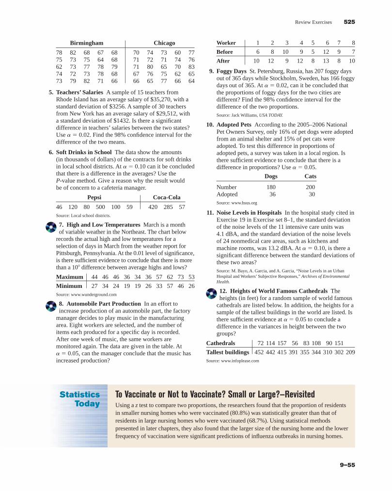
Review Exercises 525
9–55
Birmingham Chicago
78 82 68 67 68 70 74 73 60 7775 73 75 64 68 71 72 71 74 7662 73 77 78 79 71 80 65 70 8374 72 73 78 68 67 76 75 62 6573 79 82 71 66 66 65 77 66 64
5. Teachers’ Salaries A sample of 15 teachers fromRhode Island has an average salary of $35,270, with astandard deviation of $3256. A sample of 30 teachersfrom New York has an average salary of $29,512, witha standard deviation of $1432. Is there a significantdifference in teachers’ salaries between the two states?Use a � 0.02. Find the 98% confidence interval for thedifference of the two means.
6. Soft Drinks in School The data show the amounts(in thousands of dollars) of the contracts for soft drinksin local school districts. At a � 0.10 can it be concludedthat there is a difference in the averages? Use theP-value method. Give a reason why the result wouldbe of concern to a cafeteria manager.
Pepsi Coca-Cola
46 120 80 500 100 59 420 285 57Source: Local school districts.
7. High and Low Temperatures March is a monthof variable weather in the Northeast. The chart below
records the actual high and low temperatures for aselection of days in March from the weather report forPittsburgh, Pennsylvania. At the 0.01 level of significance,is there sufficient evidence to conclude that there is morethan a 10 difference between average highs and lows?
Maximum 44 46 46 36 34 36 57 62 73 53
Minimum 27 34 24 19 19 26 33 57 46 26Source: www.wunderground.com
8. Automobile Part Production In an effort toincrease production of an automobile part, the factory
manager decides to play music in the manufacturingarea. Eight workers are selected, and the number ofitems each produced for a specific day is recorded.After one week of music, the same workers aremonitored again. The data are given in the table. Ata � 0.05, can the manager conclude that the music hasincreased production?
Worker 1 2 3 4 5 6 7 8
Before 6 8 10 9 5 12 9 7
After 10 12 9 12 8 13 8 10
9. Foggy Days St. Petersburg, Russia, has 207 foggy daysout of 365 days while Stockholm, Sweden, has 166 foggydays out of 365. At a � 0.02, can it be concluded thatthe proportions of foggy days for the two cities aredifferent? Find the 98% confidence interval for thedifference of the two proportions.Source: Jack Williams, USA TODAY.
10. Adopted Pets According to the 2005–2006 NationalPet Owners Survey, only 16% of pet dogs were adoptedfrom an animal shelter and 15% of pet cats wereadopted. To test this difference in proportions ofadopted pets, a survey was taken in a local region. Isthere sufficient evidence to conclude that there is adifference in proportions? Use a � 0.05.
Dogs Cats
Number 180 200Adopted 36 30Source: www.hsus.org
11. Noise Levels in Hospitals In the hospital study cited inExercise 19 in Exercise set 8–1, the standard deviationof the noise levels of the 11 intensive care units was4.1 dBA, and the standard deviation of the noise levelsof 24 nonmedical care areas, such as kitchens andmachine rooms, was 13.2 dBA. At a � 0.10, is there asignificant difference between the standard deviations ofthese two areas?Source: M. Bayo, A. Garcia, and A. Garcia, “Noise Levels in an UrbanHospital and Workers’ Subjective Responses,” Archives of EnvironmentalHealth.
12. Heights of World Famous Cathedrals Theheights (in feet) for a random sample of world famous
cathedrals are listed below. In addition, the heights for asample of the tallest buildings in the world are listed. Isthere sufficient evidence at a� 0.05 to conclude adifference in the variances in height between the twogroups?
Cathedrals 72 114 157 56 83 108 90 151
Tallest buildings 452 442 415 391 355 344 310 302 209Source: www.infoplease.com
StatisticsToday
To Vaccinate or Not to Vaccinate? Small or Large?—RevisitedUsing a z test to compare two proportions, the researchers found that the proportion of residentsin smaller nursing homes who were vaccinated (80.8%) was statistically greater than that ofresidents in large nursing homes who were vaccinated (68.7%). Using statistical methodspresented in later chapters, they also found that the larger size of the nursing home and the lowerfrequency of vaccination were significant predictions of influenza outbreaks in nursing homes.
blu34978_ch09.qxd 8/13/08 6:06 PM Page 525
Confirming Pages
526 Chapter 9 Testing the Difference Between Two Means, Two Proportions, and Two Variances
9–56
The Data Bank is found in Appendix D, or on theWorld Wide Web by following links fromwww.mhhe.com/math/stat/bluman/
1. From the Data Bank, select a variable and compare themean of the variable for a random sample of at least30 men with the mean of the variable for the randomsample of at least 30 women. Use a z test.
2. Repeat the experiment in Exercise 1, using a differentvariable and two samples of size 15. Compare the meansby using a t test.
3. Compare the proportion of men who are smokers withthe proportion of women who are smokers. Use the datain the Data Bank. Choose random samples of size 30 ormore. Use the z test for proportions.
4. Select two samples of 20 values from the data in DataSet IV in Appendix D. Test the hypothesis that the meanheights of the buildings are equal.
5. Using the same data obtained in Exercise 4, test thehypothesis that the variances are equal.
Data Analysis
Determine whether each statement is true or false. If thestatement is false, explain why.
1. When you are testing the difference between twomeans for small samples, it is not important todistinguish whether the samples are independent ofeach other.
2. If the same diet is given to two groups of randomlyselected individuals, the samples are considered to bedependent.
3. When computing the F test value, you always place thelarger variance in the numerator of the fraction.
4. Tests for variances are always two-tailed.
Select the best answer.
5. To test the equality of two variances, you would use a(n) test.a. z c. Chi-squareb. t d. F
6. To test the equality of two proportions, you would usea(n) test.a. z c. Chi-squareb. t d. F
7. The mean value of the F is approximately equal to
a. 0 c. 1b. 0.5 d. It cannot be determined.
8. What test can be used to test the difference between twosample means when the population variances are known?
a. z c. Chi-squareb. t d. F
Complete these statements with the best answer.
9. If you hypothesize that there is no difference betweenmeans, this is represented as H0: .
10. When you are testing the difference between twomeans, the test is used when the populationvariances are not known.
11. When the t test is used for testing the equality of twomeans, the populations must be .
12. The values of F cannot be .
13. The formula for the F test for variances is .
For each of these problems, perform the following steps.
a. State the hypotheses and identify the claim.b. Find the critical value(s).c. Compute the test value.d. Make the decision.e. Summarize the results.
Use the traditional method of hypothesis testing unlessotherwise specified.
14. Cholesterol Levels A researcher wishes to see if thereis a difference in the cholesterol levels of two groups ofmen. A random sample of 30 men between the ages of25 and 40 is selected and tested. The average level is223. A second sample of 25 men between the ages of 41and 56 is selected and tested. The average of this groupis 229. The population standard deviation for bothgroups is 6. At a� 0.01, is there a difference in thecholesterol levels between the two groups? Find the99% confidence interval for the difference of thetwo means.
15. Apartment Rental Fees The data shown are therental fees (in dollars) for two random samples of
apartments in a large city. At a � 0.10, can it be con-cluded that the average rental fee for apartments in theEast is greater than the average rental fee in the West?Assume s1 � 119 and s2 � 103.
Chapter Quiz
blu34978_ch09.qxd 8/13/08 6:06 PM Page 526
Confirming Pages
Chapter Quiz 527
9–57
East West
495 390 540 445 420 525 400 310 375 750410 550 499 500 550 390 795 554 450 370389 350 450 530 350 385 395 425 500 550375 690 325 350 799 380 400 450 365 425475 295 350 485 625 375 360 425 400 475275 450 440 425 675 400 475 430 410 450625 390 485 550 650 425 450 620 500 400685 385 450 550 425 295 350 300 360 400
Source: Pittsburgh Post-Gazette.
16. Prices of Low-Calorie Foods The average price of asample of 12 bottles of diet salad dressing taken fromdifferent stores is $1.43. The standard deviation is$0.09. The average price of a sample of 16 low-caloriefrozen desserts is $1.03. The standard deviation is$0.10. At a � 0.01, is there a significant difference inprice? Find the 99% confidence interval of thedifference in the means.
17. Jet Ski Accidents The data shown represent thenumber of accidents people had when using jet skis
and other types of wet bikes. At a � 0.05, can it beconcluded that the average number of accidents per yearhas increased from one period to the next?
1987–1991 1992–1996
376 650 844 1650 2236 30021162 1513 4028 4010
Source: USA TODAY.
18. Salaries of Chemists A sample of 12 chemists fromWashington state shows an average salary of $39,420with a standard deviation of $1659, while a sample of26 chemists from New Mexico has an average salaryof $30,215 with a standard deviation of $4116. Is therea significant difference between the two states inchemists’ salaries at a � 0.02? Find the 98% confidenceinterval of the difference in the means.
19. Family Incomes The average income of 15 familieswho reside in a large metropolitan East Coast city is$62,456. The standard deviation is $9652. The averageincome of 11 families who reside in a rural area ofthe Midwest is $60,213, with a standard deviation of$2009. At a � 0.05, can it be concluded that thefamilies who live in the cities have a higher incomethan those who live in the rural areas? Use the P-valuemethod.
20. Mathematical Skills In an effort to improve themathematical skills of 10 students, a teacher provides
a weekly 1-hour tutoring session for the students. Apretest is given before the sessions, and a posttest isgiven after. The results are shown here. At a � 0.01,can it be concluded that the sessions help to improvethe students’ mathematical skills?
Student 1 2 3 4 5 6 7 8 9 10
Pretest 82 76 91 62 81 67 71 69 80 85
Posttest 88 80 98 80 80 73 74 78 85 93
21. Egg Production To increase egg production, afarmer decided to increase the amount of time the
lights in his hen house were on. Ten hens were selected,and the number of eggs each produced was recorded.After one week of lengthened light time, the same henswere monitored again. The data are given here. At a �0.05, can it be concluded that the increased light timeincreased egg production?
Hen 1 2 3 4 5 6 7 8 9 10
Before 4 3 8 7 6 4 9 7 6 5
After 6 5 9 7 4 5 10 6 9 6
22. Factory Worker Literacy Rates In a sample of80 workers from a factory in city A, it was found that5% were unable to read, while in a sample of 50 workersin city B, 8% were unable to read. Can it be concludedthat there is a difference in the proportions ofnonreaders in the two cities? Use a � 0.10. Findthe 90% confidence interval for the difference of thetwo proportions.
23. Male Head of Household A recent survey of 200households showed that 8 had a single male as thehead of household. Forty years ago, a survey of 200households showed that 6 had a single male as the headof household. At a � 0.05, can it be concluded that theproportion has changed? Find the 95% confidenceinterval of the difference of the two proportions. Doesthe confidence interval contain 0? Why is this importantto know?Source: Based on data from the U.S. Census Bureau.
24. Money Spent on Road Repair A politician wishes tocompare the variances of the amount of money spent forroad repair in two different counties. The data are givenhere. At a � 0.05, is there a significant difference in thevariances of the amounts spent in the two counties? Usethe P-value method.
County A County B
s1 � $11,596 s2 � $14,837n1 � 15 n2 � 18
25. Heights of Basketball Players A researcher wants tocompare the variances of the heights (in inches) of four-year college basketball players with those of players injunior colleges. A sample of 30 players from each typeof school is selected, and the variances of the heights foreach type are 2.43 and 3.15, respectively. At a � 0.10,is there a significant difference between the variances ofthe heights in the two types of schools?
blu34978_ch09.qxd 8/13/08 6:06 PM Page 527
Confirming Pages
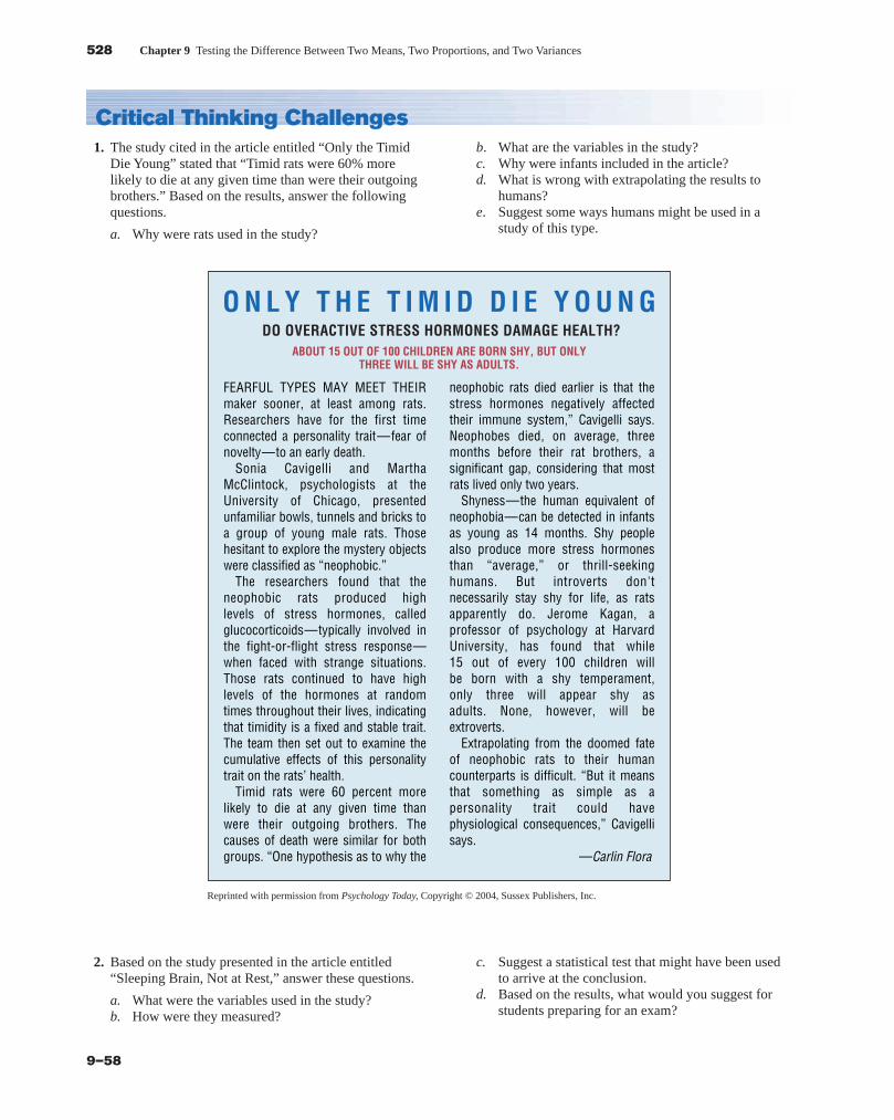
528 Chapter 9 Testing the Difference Between Two Means, Two Proportions, and Two Variances
9–58
2. Based on the study presented in the article entitled“Sleeping Brain, Not at Rest,” answer these questions.
a. What were the variables used in the study?b. How were they measured?
c. Suggest a statistical test that might have been usedto arrive at the conclusion.
d. Based on the results, what would you suggest forstudents preparing for an exam?
O N L Y T H E T I M I D D I E Y O U N G
ABOUT 15 OUT OF 100 CHILDREN ARE BORN SHY, BUT ONLYTHREE WILL BE SHY AS ADULTS.
DO OVERACTIVE STRESS HORMONES DAMAGE HEALTH?
FEARFUL TYPES MAY MEET THEIR maker sooner, at least among rats. Researchers have for the first time connected a personality trait—fear of novelty—to an early death.
Sonia Cavigelli and Martha McClintock, psychologists at the University of Chicago, presented unfamiliar bowls, tunnels and bricks to a group of young male rats. Those hesitant to explore the mystery objects were classified as “neophobic.”
The researchers found that the neophobic rats produced high levels of stress hormones, called glucocorticoids—typically involved in the fight-or-flight stress response— when faced with strange situations. Those rats continued to have high levels of the hormones at random times throughout their lives, indicating that timidity is a fixed and stable trait. The team then set out to examine the cumulative effects of this personality trait on the rats’ health.
Timid rats were 60 percent more likely to die at any given time than were their outgoing brothers. The causes of death were similar for both groups. “One hypothesis as to why the
neophobic rats died earlier is that the stress hormones negatively affected their immune system,” Cavigelli says. Neophobes died, on average, three months before their rat brothers, a significant gap, considering that most rats lived only two years.
Shyness—the human equivalent of neophobia—can be detected in infants as young as 14 months. Shy people also produce more stress hormones than “average,” or thrill-seeking humans. But introverts don't necessarily stay shy for life, as rats apparently do. Jerome Kagan, a professor of psychology at Harvard University, has found that while 15 out of every 100 children will be born with a shy temperament, only three will appear shy as adults. None, however, will be extroverts.
Extrapolating from the doomed fate of neophobic rats to their human counterparts is difficult. “But it means that something as simple as a personality trait could have physiological consequences,” Cavigelli says.
—Carlin Flora
Reprinted with permission from Psychology Today, Copyright © 2004, Sussex Publishers, Inc.
1. The study cited in the article entitled “Only the TimidDie Young” stated that “Timid rats were 60% morelikely to die at any given time than were their outgoingbrothers.” Based on the results, answer the followingquestions.
a. Why were rats used in the study?
b. What are the variables in the study?c. Why were infants included in the article?d. What is wrong with extrapolating the results to
humans?e. Suggest some ways humans might be used in a
study of this type.
Critical Thinking Challenges
blu34978_ch09.qxd 8/13/08 6:06 PM Page 528
Confirming Pages
Answers to Applying the Concepts 529
9–59
Use a significance level of 0.05 for all tests below.
1. Business and Finance Use the data collected in dataproject 1 of Chapter 2 to complete this problem. Test theclaim that the mean earnings per share for Dow Jonesstocks are greater than for NASDAQ stocks.
2. Sports and Leisure Use the data collected in dataproject 2 of Chapter 7 regarding home runs for thisproblem. Test the claim that the mean number of homeruns hit by the American League sluggers is the sameas the mean for the National League.
3. Technology Use the cell phone data collected for dataproject 2 in Chapter 8 to complete this problem. Test theclaim that the mean length for outgoing calls is the sameas that for incoming calls. Test the claim that thestandard deviation for outgoing calls is more than thatfor incoming calls.
4. Health and Wellness Use the data regarding BMIthat were collected in data project 6 of Chapter 7 tocomplete this problem. Test the claim that the meanBMI for males is the same as that for females. Test theclaim that the standard deviation for males is the sameas that for females.
5. Politics and Economics Use data from the lastPresidential election to categorize the 50 states as “red”or “blue” based on who was supported for President inthat state, the Democratic or Republican candidate. Usethe data collected in data project 5 of Chapter 2regarding income. Test the claim that the mean incomesfor red states and blue states are equal.
6. Your Class Use the data collected in data project 6 ofChapter 2 regarding heart rates. Test the claim thatthe heart rates after exercise are more variable than theheart rates before exercise.
Data Projects
SLEEPING BRAIN, NOT AT RESTRegions of the brain that have spent
the day learning sleep more heavily at night.
In a study published in the journal Nature, Giulio Tononi, a psychiatrist at the University of Wisconsin– Madison, had subjects perform a simple point-and-click task with a computer adjusted so that its cursor didn’t track in the right direction. Afterward, the subjects’ brain waves were recorded while they slept, then examined for “slow wave” activity, a
kind of deep sleep.Compared with people who’d
completed the same task with normal cursors, Tononi’s subjects showed elevated slow wave activity in brain areas associated with spatial orientation, indicating that their brains were adjusting to the day’s learning by making cellular-level changes. In the morning, Tononi’s subjects performed their tasks better than they had before going to sleep.
—Richard A. Love
Reprinted with permission from Psychology Today, Copyright © 2004, Sussex Publishers, Inc.
Section 9–1 Home Runs
1. The population is all home runs hit by major leaguebaseball players.
2. A cluster sample was used.
3. Answers will vary. While this sample is not representa-tive of all major league baseball players per se, it doesallow us to compare the leaders in each league.
4. H0: m1 � m2 and H1: m1 � m2
5. Answers will vary. Possible answers include the 0.05and 0.01 significance levels.
6. We will use the z test for the difference in means.
7. Our test statistic is and our
P-value is 0.3124.
8. We fail to reject the null hypothesis.
z �44.75 � 42.88
28.82
40�
7.82
40
� 1.01,
Answers to Applying the Concepts
blu34978_ch09.qxd 8/13/08 6:06 PM Page 529
Confirming Pages
530 Chapter 9 Testing the Difference Between Two Means, Two Proportions, and Two Variances
9–60
9. There is not enough evidence to conclude that thereis a difference in the number of home runs hit byNational League versus American League baseballplayers.
10. Answers will vary. One possible answer is thatsince we do not have a random sample of data fromeach league, we cannot answer the original questionasked.
11. Answers will vary. One possible answer is that we couldget a random sample of data from each league from arecent season.
Section 9–2 Too Long on the Telephone
1. These samples are independent.
2. There were 56 � 2 � 58 people in the study.
3. We compare the P-value of 0.06317 to the significancelevel to check if the null hypothesis should be rejected.
4. The P-value of 0.06317 also gives the probability of atype I error.
5. The F value of 3.07849 is the result of dividing the twosample variances.
6. Since two critical values are shown, we know that atwo-tailed test was done.
7. Since the P-value of 0.06317 is greater than thesignificance value of 0.05, we fail to reject the nullhypothesis and find that we do not have enoughevidence to conclude that there is a difference in thelengths of telephone calls made by employees in thetwo divisions of the company.
8. If the significance level had been 0.10, we would haverejected the null hypothesis, since the P-value wouldhave been less than the significance level.
Section 9–3 Air Quality
1. The purpose of the study is to determine if the airquality in the United States has changed over the past2 years.
2. These are dependent samples, since we have tworeadings from each of 10 metropolitan areas.
3. The hypotheses we will test are and
4. We will use the 0.05 significance level and criticalvalues of t � �2.262.
5. We will use the t test for dependent samples.
6. There are 10 � 1 � 9 degrees of freedom.
H1: mD � 0.H0: mD � 0
7. Our test statistic is We fail
to reject the null hypothesis and find that there is notenough evidence to conclude that the air quality in theUnited States has changed over the past 2 years.
8. No, we could not use an independent means testsince we have two readings from eachmetropolitan area.
9. Answers will vary. One possible answer is that thereare other measures of air quality that we could haveexamined to answer the question.
Section 9–4 Smoking and Education
1. Our hypotheses are and
2. At the 0.05 significance level, our critical values are
3. We will use the z test for the difference betweenproportions.
4. To complete the statistical test, we would need thesample sizes.
5. Knowing the sample sizes were 1000, we can nowcomplete the test.
6. Our test statistic is
9.40, and our P-value is very close to zero. We rejectthe null hypothesis and find that there is enoughevidence to conclude that there is a difference in theproportions of high school graduates and collegegraduates who smoke.
Section 9–5 Variability and AutomaticTransmissions
1. The null hypothesis is that the variances are the same: ( ).
2. We will use an F test.
3. The value of the test statistic is
and the P-value is 0.0008. There is a significantdifference in the variability of the prices between thetwo countries.
4. Small sample sizes are highly impacted by outliers.
5. The degrees of freedom for the numerator anddenominator are both 5.
6. Yes, two sets of data can center on the same mean buthave very different standard deviations.
F �s2
1
s22
�514.82
77.72 � 43.92,
H1: s12 � s2
2H0: s12 � s2
2
z �0.323 � 0.145
2�0.234��0.766�� 11000
�1
1000� �
z � �1.96.
H1: p1 � p2.H0: p1 � p2
t ��6.7 � 0
11.27�210 � �1.879.
blu34978_ch09.qxd 8/13/08 6:06 PM Page 530
Confirming Pages

Hypothesis-Testing Summary 1 531
9–61
1. Comparison of a sample mean with a specificpopulation mean.
Example: H0: m � 100
a. Use the z test when s is known:
b. Use the t test when s is unknown:
2. Comparison of a sample variance or standard deviationwith a specific population variance or standarddeviation.
Example: H0: s2 � 225
Use the chi-square test:
3. Comparison of two sample means.
Example: H0: m1 � m2
a. Use the z test when the population variances areknown:
b. Use the t test for independent samples when thepopulation variances are unknown and assumethe sample variances are unequal:
with d.f. � the smaller of n1 � 1 or n2 � 1.
t ��X1 � X2� � �m1 � m2�
As2
1
n1�
s22
n2
z ��X1 � X2� � �m1 � m2�
As2
1
n1�s2
2
n2
x2 ��n � 1�s2
s2 with d.f. � n � 1
t � X � m
s �2n with d.f. � n � 1
z � X � m
s �2n
c. Use the t test for means for dependent samples:
Example: H0: mD � 0
where n � number of pairs.
4. Comparison of a sample proportion with a specificpopulation proportion.
Example: H0: p � 0.32
Use the z test:
5. Comparison of two sample proportions.
Example: H0: p1 � p2
Use the z test:
where
6. Comparison of two sample variances or standarddeviations.
Example: H0:
Use the F test:
where
� larger variance d.f.N. � n1 � 1
� smaller variance d.f.D. � n2 � 1s22
s21
F �s2
1
s22
s21 � s2
2
q � 1 � p p̂2 �X2
n2
p �X1 � X2
n1 � n2 p̂1 �
X1
n1
z �� p̂1 � p̂2� � �p1 � p2�
A p q ¢ 1n1
�1n2≤
z �X � m
s or z �
p̂ � p
2pq�n
t � D � mD
sD �2n with d.f. � n � 1
Hypothesis-Testing Summary 1
blu34978_ch09.qxd 8/13/08 6:06 PM Page 531
Confirming Pages

blu34978_ch09.qxd 8/13/08 6:06 PM Page 532
Confirming Pages