testing inequality constrained hypotheses in sem models · hypotheses do not differ in model fit;...
TRANSCRIPT

Structural Equation Modeling, 17:443–463, 2010
Copyright © Taylor & Francis Group, LLC
ISSN: 1070-5511 print/1532-8007 online
DOI: 10.1080/10705511.2010.489010
Testing Inequality Constrained Hypothesesin SEM Models
Rens van de Schoot and Herbert HoijtinkDepartment of Methods and Statistics
Utrecht University, The Netherlands
Maja DekovicDepartment of Child and Adolescent Studies
Utrecht University, The Netherlands
Researchers often have expectations that can be expressed in the form of inequality constraints
among the parameters of a structural equation model. It is currently not possible to test these
so-called informative hypotheses in structural equation modeling software. We offer a solution to
this problem using Mplus. The hypotheses are evaluated using plug-in p values with a calibrated
alpha level. The method is introduced and its utility is illustrated by means of an example.
Order-restricted inference has been studied in the frequentist framework (see, e.g., Barlow,
Bartholomew, Bremner, & Brunk, 1972; Robertson, Wright, & Dykstra, 1988; Silvapulle &
Sen, 2004) as well as in the Bayesian framework (e.g., Hoijtink, Klugkist, & Boelen, 2008;
Klugkist, Laudy, & Hoijtink, 2005). However, testing order constraints has received relatively
little attention in the structural equation modeling (SEM) literature (Gonzalez & Griffin,
2001; Stoel, Galindo-Garre, Dolan, & Van den Wittenboer, 2006). SEM is often used and
its attractiveness is largely due to its flexibility in specifying and testing hypotheses among
both observed and latent variables in multiple groups.
SEM software can be used to impose inequality constraints among the parameters of
interest. More specifically, to evaluate a research question, model parameters such as regression
coefficients can be constrained to being greater or smaller than either a fixed value or other
regression coefficients. We call hypotheses that contain inequality constraints informative
hypotheses. Mplus (Muthén & Muthén, 2007) allows for such user-specified constraints and
order constraint parameter estimation is available. The problem is that a null hypothesis test
for the evaluation of an informative hypothesis is lacking in SEM software.
Correspondence should be addressed to Rens van de Schoot, Department of Methods and Statistics, Utrecht
University, P.O. Box 80.140, 3508TC, Utrecht, The Netherlands. E-mail: [email protected]
443

444 VAN DE SCHOOT, HOIJTINK, DEKOVIC
We offer a solution to this problem based on the parametric bootstrap method available in
Mplus. Plug-in p values are obtained using a likelihood ratio test. The performance of these p
values is evaluated and we show that the alpha level should be calibrated. Using some examples,
we demonstrate how this can be done.
CONSTRAINT PARAMETER ESTIMATION AND HYPOTHESIS TESTING
Ritov and Gilula (1993) proposed to obtain maximum likelihood estimates of order-restricted
models by a pooling adjacent violators algorithm (see also Robertson et al., 1988, p. 56). The
procedure in Mplus (Muthén & Muthén, 2007), the slacking parameter method, is based on
the solution of Ritov and Gilula. The core of the algorithm is estimating the parameters via
the maximum likelihood method such that the likelihood is maximized using the sequential
quadratic programming method (Han, 1977). In this method the parameters that contain inequal-
ity constraints are updated in an iterative process where inequality constraints are treated as
equality constraints whenever the estimates do not fit the constraints imposed on the parameters.
This is done by the introduction of “slack” parameters into the model. See Schoenberg (1997)
for more details.
How to test inequality constraint hypotheses has mainly been studied outside the SEM
model. See Barlow et al. (1972), Robertson et al. (1988), and Silvapulle and Sen (2004)
for a comprehensive overview. In 2002 the Journal of Statistical Planning and Inference
published a special issue on testing inequality constraint hypotheses (Berger & Ivanova, 2002;
Chongcharoen, Singh, & Wright, 2002; Khalil, Saikali, & Berger, 2002; Lee & Yan, 2002;
Perlman & Wu, 2002a, 2002b; Sampson & Singh, 2002; Sen & Silvapulle, 2002; Silvapulle,
Silvapulle, & Basawa, 2002), but none of these articles discussed constraints in SEM models.
Testing informative hypotheses for SEM models has been described by Stoel et al. (2006). In
this study, constraints were imposed on variance terms to obtain only positive values. Hypothesis
tests were performed to test the benefit of these constraints (see also Gonzalez & Griffin, 2001).
Also, Tsonaka and Moustaki (2007) described testing parameter constraints in SEM models.
They specifically described factor analysis where a parametric bootstrap was performed to
obtain the results. However, they only considered a comparison between a constrained and an
unconstrained model. In this study we also focus on constraint hypothesis testing within the
SEM model, and although we present examples of a path model, our solution is not limited to
these kind of models. We also show that the alpha values used in constraint hypothesis testing
need to be calibrated, which is not done in the studies just described.
In almost all of the literature already described, the likelihood ratio test (LRT) is used to test
the inequality constraint hypothesis at hand. The null distribution of this test is a chi-square
distribution with degrees of freedom equal to the difference between the number of parameters
of the models under comparison (Bollen, 1989). An important result from the work of Barlow
et al. (1972), Robertson et al. (1988), and Silvapulle and Sen (2004) is that one of the regularity
conditions of the LRT does not hold when testing inequality constraint hypotheses (see also
Andrews, 1996, 2000; Ritov & Gilula, 1993; Stoel et al., 2006). Consequently, the asymptotic
distribution of the LRT is no chi-square distribution and its p value cannot straightforwardly
be computed.

TESTING INEQUALITY CONSTRAINED HYPOTHESES 445
Moreover, model selection criteria, such as the Akaike’s Information Criterion or Bayesian
Information Criterion, cannot be used to distinguish between statistical models with inequality
constraints between the parameters of interest. These criteria use the likelihood evaluated in its
maximum as a measure of model fit, and the number of parameters of the model as a measure of
complexity. The problem is that model selection criteria cannot distinguish between hypotheses
when these hypotheses do not differ in model fit, but only in the number of constraints imposed
on the parameters of interest.
For example, consider the hypothesis f™1 �™2g < ™3 > 0 where ™1 : : : ™3 denote, for example,
mean scores on some variable. Furthermore, suppose we want to compare this informative
hypothesis to an unconstrained hypothesis where the parameters are allowed to have any
value. Suppose the unconstraint parameter estimates fit the constraints, so that the estimated
parameters agree with f™1 � ™2g < ™3 > 0. In this case, both the constraint and unconstraint
hypotheses do not differ in model fit; that is, the maximum of the likelihood is the same for
both models. The problem is how to account for model complexity. Because the parameters are
restricted, the number of parameters used to determine model complexity is clearly not equal
to 3. So far, quantifying the number of parameters for constraint hypotheses received hardly
any attention in the literature.
In conclusion, evaluating informative hypothesis in SEM models is not possible with the LRT
or with traditional model selection criteria. Constraint parameter estimation and informative
hypothesis testing has extensively been studied, but literature for SEM models is sparse. Also,
as we show in this article, calibration of the alpha level is essential when testing inequality
constraint hypotheses. This received hardly any attention in the literature described before. We
show how informative hypotheses can be tested in SEM models using Mplus, but we first
introduce an example in which the hypotheses of interest are informative.
ILLUSTRATION: ETHNICITY AND ANTISOCIAL BEHAVIOR
The problem of testing inequality constrained hypotheses in SEM and its solution is illustrated
using the following example. Dekovic, Wissink, and Meijer (2004) investigated whether the
leading theories about antisocial behavior in the dominant culture of adolescents can be
generalized to members of different ethnic groups. For this example the dominant culture is the
Dutch culture, which is compared to the Moroccan, Turkish, and Surinamese cultures in the
Netherlands. Three aspects of the parent–adolescent relationship were assessed: positive quality
of the relationship (affection and intimacy), negative quality of the relationship (antagonism
and conflict), and disclosure (how much adolescents tell the parents). The sample consists of
603 adolescents (M age D 14.4, range D 14–16 years); 68% of the adolescents are Dutch
(n D 407), 11% are Moroccan (n D 68), 13% are Turkish (n D 79), and 8% are Surinamese
(n D 49). Adolescents were classified into these ethnic categories according to their responses
on a single item in the questionnaire: “What ethnical group best describes you?” Using these
data we present three examples where the hypothesis under investigation is informative.
The structural equation model used here is given by
ygi D Bgy
gi C �gx
gi C —
gi with xi � N.�g
x ; ˆg/ (1)

446 VAN DE SCHOOT, HOIJTINK, DEKOVIC
where, if q is the number of dependent variables, r is the number of independent variables,
g D 1; : : : ; G denotes group membership, and i D 1; : : : ; I denote persons, then ygi is a
q � 1 vector of dependent variables for person i within group g, Bg is a q � q matrix of
regression coefficients between ys where the diagonal must consist of zeros, xi is a r � 1
vector of independent variables, �gx is a r � 1 vector of means for each independent variable
with covariance matrix ˆg, �g is q�r matrix of regression coefficients between ys and xs, and
—gi is q � 1 vector with error terms that is assumed to have a multivariate-normal distribution,
—gi � N.0; ‰g/, which is independent of y and x. Under these assumptions, the observed y i
and xi have a multivariate-normal distribution with
�
ygi
xgi
�
� NqCr
�
�gy
�gx
; †g
�
(2)
where † represents the implied covariance matrix that is given by
†g D
2
6
6
4
†gyy †
gxy
.q�q/ .r�q/
†gyx †
gxx
.q�r/ .r�r/
3
7
7
5
(3)
with I being the identity matrix and
†gxx D ˆg
†g
yy0 D .I � Bg/�1.� gˆg� 0g C ‰g/.I � B
g/�10
†gxy D ˆg�g.I � B
g/�10
:
(4)
Let ™ D f™1; ™2g with ™1 D fB1; : : : ; BG ; �1; : : : ; �Gg and ™2 D fˆ1; : : : ; ˆG ; ‰1; : : : ; ‰Gg.
Then, the likelihood function can be given by
log f .y; x j ™/ DPG
gD1.Ng
N/F
gML
�
Sg ; †g
�
(5)
where Ng is the sample size for group g, Sg is the sample covariance matrix among the
observed variables in group g, y D fy1; : : : ; yN g, x D fx1; : : : ; xN g and where FgML is given
by
Fg
ML D log j †g j Ctrh
Sg†g�1
� log j Sg j �.q C r/
i
(6)
We consider two types of hypothesis tests (Silvapulle & Sen, 2004), Type A is of the form
H0 W A™1 D c
H1 W A™1 > c;(7)
and Type B is of the form
H0 W A™1 > c
H1 W unconstrained;(8)

TESTING INEQUALITY CONSTRAINED HYPOTHESES 447
where the unconstrained model refers to a model without any constraints imposed on the
parameters and where, if m is the number of inequality constraints imposed on the model and
k the number of parameters involved, A is an m � k matrix of known constants, and c is an
m � 1 vector of known constants. More specific examples will be given in the sequel.
Example 1: Simple Regression
The first example is a simple regression model where levels of antisocial behavior are regressed
on either a negative or positive relation with the parent and adolescent disclosure (see Figure
1), where B D 0 and
� D�
”1 ”2 ”3
�
; (9)
‰ D�
§1
�
; (10)
ˆ D
2
4
¥11
¥12 ¥22
¥13 ¥23 ¥33
3
5 : (11)
Note that this model is based on the total sample, therefore the superscript g is not needed.
Dekovic et al. (2004) stated that adolescent disclosure is the strongest predictor of antisocial
behavior, followed by either a negative or positive relation with the parent (see also Dishion
& McMahon, 1998). We therefore hypothesize that the regression coefficients ”1 and ”2 are
smaller than ”3. Using
A D
�
�1 0 1
0 �1 1
�
; (12)
™1 D
2
4
”1
”2
”3
3
5 ; (13)
c D
�
0
0
�
; (14)
FIGURE 1 Path model among relationship characteristics, disclosure, and prevalence of antisocial behavior.

448 VAN DE SCHOOT, HOIJTINK, DEKOVIC
the hypotheses tested for this example with m D 2, are for Type A
H0 W
versus
H1 W
�
”3 � ”1 D 0
”3 � ”2 D 0
�
�
”3 � ”1 > 0
”3 � ”2 > 0
�
;
(15)
and for Type B
H0 W
versus
H1 W
�
”3 � ”1 > 0
”3 � ”2 > 0
�
�
”3 ; ”1
”3 ; ”2
�
:
(16)
Note that H1 in Equation 16 can also be written as f”1 ; ”2g < ”3. This type of notation will
be used in the remainder of this article. We used Mplus version 5 (Muthén & Muthén, 2007)
to estimate the unconstrained and constrained regression coefficients (see Table 1). As can be
seen in this table, the unconstrained estimate of ”2 is not smaller than ”3. Consequently, the
constrained estimates of ”2 and ”3 are set equal by the introduction of a “slack” parameter
(see the lower panel of Table 1).
Example 2: Multigroup Analysis
Research about the nature and impact of antisocial behavior is dominated by studies conducted
with White, Western, middle-class adolescents (Dekovic et al., 2004). It could be questioned
whether the model in Figure 1 is the same for different ethnic groups living in The Netherlands:
Dutch (indicated by g D 1), Turkish (g D 2), Moroccan (g D 3), and Surinamese adolescents
TABLE 1
Regression Coefficients for Example 1
Coefficient B SE
Unconstrained”1 .06 .02”2 .24 .03
”3 .23 .03Constrained
”1 .06 .02”2 .235 .03”3 .235 .03

TESTING INEQUALITY CONSTRAINED HYPOTHESES 449
(g D 4), where B D 0 and
�1 D Œ ”11 ”1
2 ”13 �
:::
�4 D Œ ”41 ”4
2 ”43 � ;
(17)
‰1 D Œ §11 �
:::
‰4 D Œ §41 � ;
(18)
ˆ1 D
:::
ˆ4 D
2
4
¥111
¥112 ¥1
22
¥113 ¥1
23 ¥133
3
5
2
4
¥411
¥412 ¥4
22
¥413 ¥4
23 ¥433
3
5 :
(19)
The null hypothesis is that the regression coefficients for the predictors of antisocial behavior
are the same for all ethnic groups (see, e.g., Greenberger & Chen, 1996):
H0 W
2
4
”11 D ”2
1 D ”31 D ”4
1
”12 D ”2
2 D ”32 D ”4
2
”13 D ”2
3 D ”33 D ”4
3
3
5 (20)
According to Dekovic et al. (2004) there are also indications in the literature that the same
risk factors have different effects in different ethnic groups, a so-called process times context
interaction phenomenon. The authors expected that cross-ethnic variations result in weaker
relations between parent–child relations and adolescent behavior compared to Dutch families.
This was mainly expected because of differences in family expectations (Phalet & Schönpflung,
2001) and differences in intergenerational conflicts due to migration (Dekovic, Noom, & Meeus,
1997). The informative hypothesis H1 is:
H1 W
2
4
”11 > f”2
1; ”31; ”4
1g”1
2 > f”22; ”3
2; ”42g
”13 > f”2
3; ”33; ”4
3g
3
5 : (21)
The hypotheses that are tested for this example are for Type A: Equation 20 versus Equation 21;
and for Type B: Equation 21 versus the unconstrained model. In Table 2 the unconstrained and
constrained regression coefficients are shown. As can be seen, not all unconstraint regression
coefficients are in agreement with the constraints of H1 in Equation 21. For example, ”2 for the
Dutch adolescents is smaller instead of higher than ”2 for Moroccan adolescents. The bottom
of Table 2 renders parameter estimates, obtained with the parameter slack method, that are in
agreement with the constraints.

450 VAN DE SCHOOT, HOIJTINK, DEKOVIC
TABLE 2
Regression Coefficients for Dutch, Moroccan, Turkish, and Surinamese
Adolescents for Example 2
Ethnicity
Coefficient Dutch Moroccan Turkish Surinamese
Unconstrained”1 .05 (.03) .12 (.09) .04 (.08) .15 (.09)”2 .28 (.03) .23 (.11) .16 (.08) .08 (.11)
”3 .20 (.04) .33 (.13) .25 (.10) .24 (.14)Constrained
”1 .06 (.02) .06 (.02) .03 (.07) .06 (.02)
”2 .28 (.03) .28 (.03) .16 (.08) .08 (.11)”3 .22 (.03) .22 (.03) .22 (.03) .16 (.12)
Note. Values in parentheses represent standard error.
Example 3: Path Model
The third example includes the variable hanging around with deviant peers. The hypothesis
states that problem behavior is not only directly predicted by disclosure and a negative or
positive relation with the parent, but is also indirectly predicted via hanging around with
deviant peers (see Figure 2), where
B D
�
0 0
“21 0
�
; (22)
� D
�
”11 ”12 ”13
”21 ”22 ”23
�
; (23)
‰ D
�
§11
0 §22
�
; (24)
ˆ D
2
4
¥11
¥12 ¥22
¥13 ¥23 ¥33
3
5 : (25)
Note that this model is based on the total sample, therefore superscript g is not needed.
As argued by Dekovic et al. (2004), children spend, especially in adolescence, more and
more time with their peers without adult supervision (see also Mounts & Steinberg, 1995).
During this period peers become the most important reference group for adolescents. Dekovic
et al. (2004) stated that especially in this period the association with deviant peers has emerged
as the most prominent predictor of problem behavior. The hypotheses tested for Example 3 are
hypothesis Type A:
H0 W “21 D ”21 D ”22 D ”23
versus
H1 W “21 > f”21 ; ”22 ; ”23g(26)

TESTING INEQUALITY CONSTRAINED HYPOTHESES 451
FIGURE 2 Path model among relationship characteristics, hanging around with deviant peers, and prevalence
of antisocial behavior.
and hypothesis Type B
H0 W “21 > f”21 ; ”22 ; ”23gversus
H1 W “21 ; ”21 ; ”22 ; ”23 :
(27)
The unconstrained and constrained regression coefficients are shown in Table 3. As can be
seen in Table 3, the constrained coefficients do not differ from their unconstrained counterparts.
Hence, the constraints imposed by the informative hypothesis are not contradicted by the data.
PARAMETRIC BOOTSTRAP
To evaluate informative hypotheses like those presented in the previous section we make
use of the parametric bootstrap. Bootstrapping is an approach for statistical inference falling
within a broader class of resampling methods (Efron & Tibshirani, 1993). Various authors have
TABLE 3
Regression Coefficients for Example 3
Coefficient B SE
Unconstrained”11 .05 .03
”12 .31 .03”13 .22 .04“21 .55 .02
Constrained”11 .05 .03
”12 .31 .03”13 .22 .04“21 .55 .02

452 VAN DE SCHOOT, HOIJTINK, DEKOVIC
suggested using the parametric bootstrap when the parameter space is restricted (Galindo-Garre
& Vermunt, 2004, 2005; Ritov & Gilula, 1993; Stoel et al., 2006; Tsonaka & Moustaki, 2007).
Bootstrap Method
The method we advocate starts with the observed data z D fy; xg and the likelihood in
Equation 5 (see Start in Figure 3). Step 1 is a parametric bootstrap from a population in which
the null hypothesis is true. First, ™ is estimated under H0 using the data z resulting in
f .zjO™H0jz/ : (28)
Using Equation 28, T bootstrap samples of size n are generated, resulting in data sets zrept ,
for t D 1; : : : ; T (see Figure 3). Then, ™ is estimated for each replicated data set under H0,
rendering
f .zrep1 jO™H0jz
rep
1/ : : : f .z
repT jO™H0jz
rep
T/ : (29)
Further, ™ is estimated under H1, rendering
f .zrep
1 jO™H1jzrep
1/ : : : f .z
rep
T jO™H1jzrep
T/ : (30)
The second step, denoted by Step 2 in Figure 3, is to repeat these computations conditional on
the observed data set and to compute f .zjO™H0jz/ and f .zjO™H1jz/.
The final step (see the lower part of the top panel of Figure 3) is to choose a test statistic,
denoted by ƒ, to investigate the compatibility of the null hypothesis with the observed data.
Like many previous studies (e.g., Barlow et al., 1972; Robertson et al., 1988, Silvapulle & Sen,
2004), we also use the LRT for evaluating the hypotheses at hand, but, as illustrated before,
we do not use a p value based on a chi-square distribution.
Because f .zj™/ is proportional to the likelihood, an LRT is performed for each replicated
data set rendering
ƒt D �2log
(
f .zrept jO™H0jz
rept
/
f .zrept jO™H1jz
rept
/
)
(31)
and for the observed data set it renders
ƒ D �2log
(
f .zjO™H0jz/
f .zjO™H1jz/
)
: (32)
Now, a p value can be computed using
p D P.ƒt > ƒ jH0; z/ : (33)
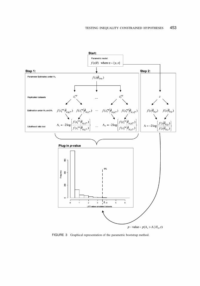
TESTING INEQUALITY CONSTRAINED HYPOTHESES 453
FIGURE 3 Graphical representation of the parametric bootstrap method.

454 VAN DE SCHOOT, HOIJTINK, DEKOVIC
It can be approximated by the proportion of LRT values from the simulated data sets that are
equal or larger than the LRT value of the observed data set, resulting in the definition of the
plug-in p value
p �
P
T
tD1 It
T; (34)
where It is an indicator function taking the value 1 if the inequality holds and 0 otherwise:
It D
�
1 if ƒt > ƒ
0 otherwise :(35)
A hypothetical distribution is illustrated in the graph in the lower part of Figure 3. To determine
whether the ƒ value from the observed data set stems from a population where the null
hypothesis is true, it has to be smaller than a chosen alpha value. Traditionally an alpha value
of .05 is used and as such the observed ƒ value has to lie on the left side of the dotted line
in Figure 3. However, as we will show in the next section, in many situations the alpha value
needs to be calibrated.
The procedure previously described can be conducted for Type A and B hypothesis testing.
The parameter estimates and likelihood values can be obtained using Mplus and we developed
R code that automatically computes the LRT values and the plug-in p value from the output
files of Mplus. Input files for all examples and R code can be downloaded from http://www.
fss.uu.nl/ms/schoot.
FREQUENCY PROPERTIES OF THE ASYMPTOTIC p VALUES
In the previous section we showed how to obtain plug-in p values for the evaluation of
informative hypotheses. An appealing property for any p value, and consequently for our
plug-in p value, is, considered as a random variable, to be asymptotically uniform [0,1] under
the null hypothesis: P.p < ’jH0/ D ’. However, in some situations exact uniformity of p
values cannot be attained (Andrews, 2000; Bayarri & Berger, 2000; Galindo-Garre & Vermunt,
2004, 2005; Stoel et al., 2006). Andrews (2000), for example, showed that the results of the
bootstrap procedure are not coherent when inequality constraints are imposed on the model
parameters. Furthermore, Galindo-Garre and Vermunt (2004) showed in a simulation study that
the parametric bootstrap can produce p values that are higher than expected.
The bootstrap procedure described in the previous section can also lead to p values that
are biased. To determine whether the actual alpha level differs from its nominal level a double
bootstrap procedure is used (Efron & Tibshirani, 1993). This procedure renders a calibrated
alpha level: P.p < ’�jH0/ D ’, where ’� denotes the calibrated alpha level.
As can be seen in Figure 4, in the double bootstrap procedure there are two stages of boot-
strapping. In Stage 1, data sets are generated using f .zjO™H0jz/. Note that we make an important
assumption here. We implicitly assume that in our procedure O™H0jz is a good approximation of
the true population values ™H0 , which are unknown. We assume that with n sufficiently large,
the true population values will be close to the estimated values f .zjO™H0jz/.

TESTING INEQUALITY CONSTRAINED HYPOTHESES 455
FIGURE 4 Graphical representation of the double bootstrap method.

456 VAN DE SCHOOT, HOIJTINK, DEKOVIC
The result of Stage 1, are S data sets (for s D 1; : : : ; S ) and the double bootstrap algorithm
amounts to treating each bootstrap sample zreps like an original data set in the second stage of
the double bootstrap procedure (see Stage 2 in Figure 4). For each first-stage data set, zreps , a
plug-in p value can be computed based on the procedure described in the previous section.
In total, S plug-in p values are computed and a hypothetical distribution of these values is
shown in the lower part of Figure 4. As can be seen, it does not have a uniform distribution, but
is skewed. In Figure 4, the 5th percentile of generated plug-in p values has a plug-in p value
of .02. That is, 5% of the p values are smaller than .02, and for example 11% of the p values
are smaller than .05. In such a case, the alpha level for evaluation of the p value computed
for the observed data set needs to be calibrated. That is, the p value should be compared to
’� D :02 instead of ’ D :05, because P.p < :02jH0/ D :05.
RESULTS FOR EXAMPLES
Example 1
To evaluate the performance of the plug-in p value for Example 1, in total four double
bootstraps are performed with S D 1,000 and T D 1,000: (a) hypothesis test Type A with
n D 50; (b) hypothesis test Type B with n D 50; (c) hypothesis test Type A with n D 640;
and (d) hypothesis test Type B with n D 640. In Figure 5 the four corresponding distributions
of plug-in p values are displayed.
As can be seen in Figure 5a and 5c the distribution for hypothesis test Type A is almost
uniform for both n D 50 and n D 640 with P.p < :048jH0/ D :05 and P.p < :046jH0/ D :05,
respectively. As was shown by Silvapulle & Sen (2004, pp. 32–33), the p values of this
statistical model and for hypothesis test Type A are uniformly distributed. Our results for small
and large sample sizes are pretty close to being uniform and the small deviations are sampling
errors. Hence, the traditional alpha level of ’ D :05 is used to evaluate the results for the
observed data set.
For hypothesis test Type B, however, the distribution is clearly not uniform, see the distri-
butions in Figure 5b and 5d. High values of the plug-in p value do not exist and low values
appear too often. For small n, P.p < :02jH0/ D :05 (see Table 4) and the alpha level for
the analysis with the observed data set needs to be calibrated, ’� D :02. Accidentally, for
large n, P.p < :048jH0/ D :05 and ’� does not need to be calibrated much, ’� D :048.
However, as can be seen in Figure 5d the distribution is clearly not uniform, for example,
P.p < :30jH0/ D :50 and P.p < :38jH0/ D :70, indicating that calibration is necessary for
different alpha levels.
To evaluate the hypotheses in Equations 15 and 16 for the observed data set, a parametric
bootstrap is performed where 1,000 data sets were generated. Each of these samples was
fitted under H0 for hypothesis test Type A and B. Based on the results shown in Table 4, it
can be concluded that for hypothesis test Type A, H0 can be rejected (p < :001; ’ D :05).
This implies that the hypothesis H0 W ”1 D ”2 D ”3 is rejected in favor of the informative
hypothesis, H1 W f”1; ”2g < ”3. Moreover, the result of hypothesis test Type B indicates that
the informative hypothesis is rejected (p < :001; ’� D :048) in favor of the unconstrained

TESTING INEQUALITY CONSTRAINED HYPOTHESES 457
(a)
(b)
FIGURE 5 Distribution of plug-in p values for Example 1: In (a) and (c), hypothesis test Type A is evaluated;
in (b) and (d) hypothesis test Type B is evaluated; in (a) and (b) n D 50; in (c) and (d) n D 640. (continued )

458 VAN DE SCHOOT, HOIJTINK, DEKOVIC
(c)
(d)
FIGURE 5 (Continued ).
model H1 W ”1; ”2; ”3. Inspection of Table 1 reveals that ”2 > ”3 and as such the unconstrained
parameter estimates do not fit either H0 W ”1 D ”2 D ”3 or H1 W f”1; ”2g < ”3.
In conclusion, levels of antisocial behavior are not evenly predicted by how much adolescents
tell the parents and by either a positive or a negative quality of the relationship with the parents
(rejection of H0). However, the expectation that disclosure is the best predictor does not hold
(rejection of H1).

TESTING INEQUALITY CONSTRAINED HYPOTHESES 459
TABLE 4
Results for the Double Bootstrap Procedure and the Parametric Bootstrap
Procedure for Examples 1 to 3
Hypothesis Test ’� ƒ Plug-In p Value
Example 1 Type A (n D 50) .048 — —Type A (n D 640) .046 42.01 <.001
Type B (n D 50) .024 — —Type B (n D 640) .048 17.41 <.001
Example 2 Type A .038 2.55 .49
Type B .058 1.07 .46Example 3 Type A .056 132.42 <.001
Type B — 0.0 >.999
Example 2
To evaluate the hypotheses for Example 2, two double bootstraps are performed to determine
the correct alpha level for hypothesis test Type A and Type B, with S D 500, T D 500, and
group sizes for group g D 1; : : : ; 4 equal to the sample sizes.
The results are shown in Table 4 and the distribution of p values is shown in Figure 6a
and b for hypothesis test Type A and B, respectively. The hypothesis H0, shown in Equation
20, cannot be rejected in favor of hypothesis H1 (p D :49; ’� D :04), shown in Equation 21.
For hypothesis test Type B the informative hypothesis cannot be rejected in favor of the
unconstrained hypothesis (p D :46; ’� D :056). So, after testing the informative hypothesis it
appears that the observed differences shown in Table 2 are too small to reject H0 shown in
Equation 20. This makes sense because confidence intervals, if computed row-wise using 1.96
times SE, overlap and as such provide a lot of support for H0 in Equation 20.
In conclusion, compared to Dutch adolescents, adolescents from different ethnic groups are
satisfied to a similar degree with their relationships with parents. Besides, Dutch adolescents
disclose as much information as adolescents from different ethnic groups.
Example 3
For Example 3, a double bootstrap was performed with S D 1,000, T D 1,000 and n D 640
for hypothesis test Type A and B. The results are shown in Table 4 and the distribution of
p values for hypothesis test Type A is shown in Figure 7. For this hypothesis test, the null
hypotheses is rejected in favor of the informative hypothesis (p < :001; ’� D :04).
For hypothesis test Type B, it appears that for all S bootstraps p D 1. This result implies
that in none of the S bootstraps did the constraint parameter estimates violate the inequality
constraints imposed on the regression coefficients. Also, for the observed data set, p D 1.
We wanted ’ to have the property P.p < :05jH0/ D :05, but for this example we observed
P.p < :05jH0/ D 0. This simulation study shows that that we cannot make an incorrect
conclusion with respect to hypothesis test Type B.
Thus, the association with deviant peers is the most prominent predictor of problem behavior.
A visual inspection of Table 3 confirms this conclusion because the unconstraint estimate “21
is larger than the unconstraint estimates of ”21; ”22, and ”23.

460 VAN DE SCHOOT, HOIJTINK, DEKOVIC
(a)
(b)
FIGURE 6 Distribution of plug-in p values for Example 2: In (a) test Type A is evaluated, and in (b) test
Type B is evaluated.

TESTING INEQUALITY CONSTRAINED HYPOTHESES 461
FIGURE 7 Distribution of plug-in p values for Example 3, test Type A.
CONCLUSION
Traditional hypotheses tests and model selection criteria are not equipped to deal with infor-
mative hypotheses formulated in terms of inequality constraints among the parameters of a
structural equation model. In this article we presented a solution for this problem using Mplus.
Some issues that need further elaboration are now discussed.
First, p values are often used in SEM and are evaluated using the traditional alpha level of
.05. Using the double bootstrap procedure we evaluated the frequency properties of the plug-in
p values resulting from our method. These results show clearly that the distribution of the
p values is not always uniform and calibration is needed. This is especially the case when
evaluating hypotheses of Type B.
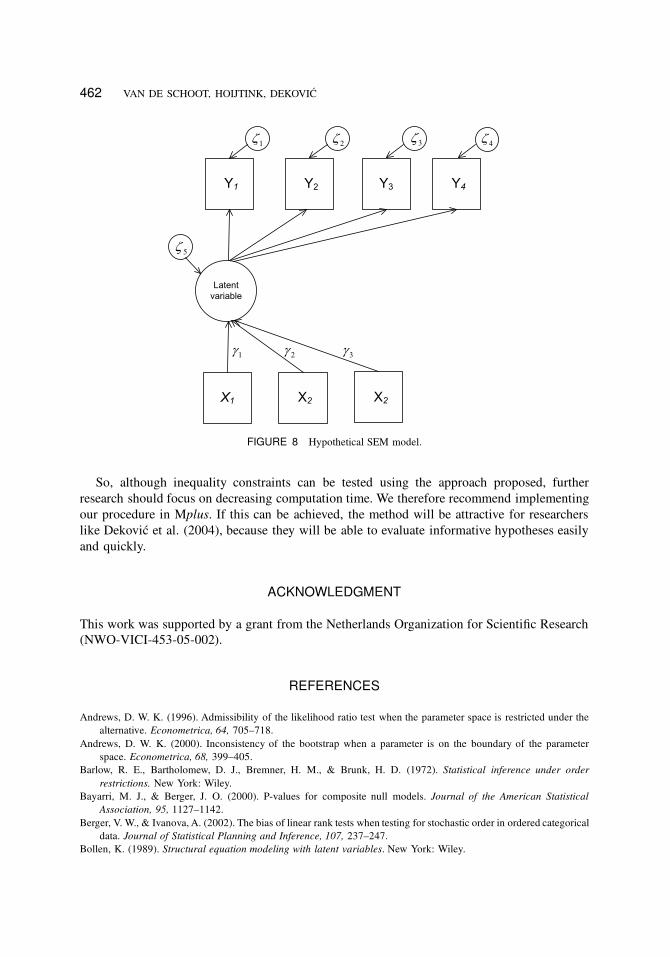
Second, we used rather simple SEM models. However, there are no technical limitations
to using inequality constraints for more complicated models in Mplus, for example, including
latent effects, second-order effects, or categorical variables. Figure 8 shows a hypothetical SEM
model with one latent variable and seven observed variables. For this model constraints could be
imposed on, for example, ”1 : : : ”3. In this article we only discussed informative hypotheses with
inequality constraints of the type ”1 > ”2 > ”3. There are, however, no technical limitations
to evaluate an informative hypothesis consisting of combinations of equality and inequality
constraints of the form ”1 > ”2 D ”3, f”1 � ”2g > 2, or f”1 � ”2g < ”3 > 1.
A limitation of the procedure is that computational time can be substantial. To compute the
examples in this article we used Pentium computers (3.20 MHz) containing two dual processors
(Mplus can deal with multiple processors) with 1 GB memory. The models for Example 1 and
3 took approximately 2 days to compute, but Example 2 took more than 2 weeks.
462 VAN DE SCHOOT, HOIJTINK, DEKOVIC
FIGURE 8 Hypothetical SEM model.
So, although inequality constraints can be tested using the approach proposed, further
research should focus on decreasing computation time. We therefore recommend implementing
our procedure in Mplus. If this can be achieved, the method will be attractive for researchers
like Dekovic et al. (2004), because they will be able to evaluate informative hypotheses easily
and quickly.
ACKNOWLEDGMENT
This work was supported by a grant from the Netherlands Organization for Scientific Research
(NWO-VICI-453-05-002).
REFERENCES
Andrews, D. W. K. (1996). Admissibility of the likelihood ratio test when the parameter space is restricted under the
alternative. Econometrica, 64, 705–718.
Andrews, D. W. K. (2000). Inconsistency of the bootstrap when a parameter is on the boundary of the parameter
space. Econometrica, 68, 399–405.
Barlow, R. E., Bartholomew, D. J., Bremner, H. M., & Brunk, H. D. (1972). Statistical inference under order
restrictions. New York: Wiley.
Bayarri, M. J., & Berger, J. O. (2000). P-values for composite null models. Journal of the American Statistical
Association, 95, 1127–1142.
Berger, V. W., & Ivanova, A. (2002). The bias of linear rank tests when testing for stochastic order in ordered categorical
data. Journal of Statistical Planning and Inference, 107, 237–247.
Bollen, K. (1989). Structural equation modeling with latent variables. New York: Wiley.

TESTING INEQUALITY CONSTRAINED HYPOTHESES 463
Chongcharoen, S., Singh, B., & Wright, F. (2002). Powers of some one-sided multivariate tests with the population
covariance matrix known up to a multiplicative constant. Journal of Statistical Planning and Inference, 107,
103–121.
Dekovic, M., Noom, M. J., & Meeus, W. (1997). Expectations regarding development during adolescence: Parental
and adolescent perceptions. Journal of Youth and Adolescence, 26, 253–272.
Dekovic, M., Wissink, I., & Meijer, A. M. (2004). The role of family and peer relations in adolescent antisocial
behaviour: Comparison of four ethnic groups. Journal of Adolescence, 27, 497–514.
Dishion, T. J., & McMahon, R. J. (1998). Parental monitoring and the prevention of child and adolescent problem
behavior: A conceptual and empirical foundation. Clinical Child and Family Psychology Review, 1, 61–75.
Efron, B., & Tibshirani, R. J. (1993). An introduction to the bootstrap. New York: Chapman & Hall.
Galindo-Garre, F., & Vermunt, J. (2004). The order-restricted association model: Two estimation algorithms and issues
in testing. Psychometrika, 69, 641–654.
Galindo-Garre, F., & Vermunt, J. (2005). Testing log-linear models with inequality constraints: A comparison of
asymptotic, bootstrap, and posterior predictive p-values. Statistica Neerlandica, 59, 82–94.
Gonzalez, R., & Griffin, D. (2001). Testing parameters in structural equation modelling: Every “one” matters. Psycho-
logical Methods, 6, 258–269.
Greenberger, E., & Chen, C. (1996). Perceived family relationships and depressed mood in early and late adolescence:
A comparison of European and Asian American. Developmental Psychology, 32, 707–716.
Han, S. (1977). A globally convergent method for nonlinear programming. Journal of Optimization Theory and
Applications, 22/23, 297–309.
Hoijtink, H., Klugkist, I., & Boelen, P. A. (Eds.). (2008). Bayesian evaluation of informative hypotheses. New York:
Springer.
Khalil, G., Saikali, R., & Berger, L. (2002). More powerful tests for the sign testing problem. Journal of Statistical
Planning and Inference, 107, 187–205.
Klugkist, I., Laudy, O., & Hoijtink, H. (2005). Inequality constrained analysis of variance: A Bayesian approach.
Psychological Methods, 10, 477–493.
Lee, C. C., & Yan, X. (2002). Chi-squared tests for and against uniform stochastic ordering on multinomial parameters.
Journal of Statistical Planning and Inference, 107, 267–280.
Mounts, N. S., & Steinberg, L. (1995). An ecological analysis of peer influence on adolescent grade point average and
drug use. Developmental Psychology, 31, 915–922.
Muthén, L. K., & Muthén, B. O. (2007). Mplus: Statistical analysis with latent variables: User’s guide. Los Angeles,
CA: Muthén & Muthén.
Perlman, M. D., & Wu, L. (2002a). A class of conditional tests for a multivariate one-sided alternative. Journal of
Statistical Planning and Inference, 107, 155–171.
Perlman, M. D., & Wu, L. (2002b). A defense of the likelihood ratio test for one-sided and order-restricted alternatives.
Journal of Statistical Planning and Inference, 107, 173–186.
Phalet, K., & Schönpflung, U. (2001). Intergenerational transmission of collectivism and achievement values in two
acculturation contexts: The case of Turkish families in Germany and Turkish and Moroccan families in the
Netherlands. Journal of Cross-Cultural Psychology, 32, 186–201.
Ritov, Y., & Gilula, Z. (1993). Analysis of contingency tables by correspondence models subject to order constraints.
Journal of the American Statistical Association, 88, 1380–1387.
Robertson, T., Wright, F. T., & Dykstra, R. L. (1988). Order restricted statistical inference. New York: Wiley.
Sampson, A. R., & Singh, H. (2002). Min and max scorings for two sample partially ordered categorical data. Journal
of Statistical Planning and Inference, 107, 219–236.
Schoenberg, S. (1997). Constrained maximum likelihood. Computational Economics, 10, 251–266.
Sen, P. K., & Silvapulle, M. J. (2002). An appraisal of some aspects of statistical inference under inequality constraints.
Journal of Statistical Planning and Inference, 107, 3–43.
Silvapulle, M. J., & Sen, P. K. (2004). Constrained statistical inference: Order, inequality, and shape constraints.
London: Wiley.
Silvapulle, M. J., Silvapulle, P., & Basawa, I. V. (2002). Tests against inequality constraints in semiparametric models.
Journal of Statistical Planning and Inference, 107, 307–320.
Stoel, R. D., Galindo-Garre, F., Dolan, C., & Van den Wittenboer, G. (2006). On the likelihood ratio test in structural
equation modeling when parameters are subject to boundary constraints. Psychological Methods, 4, 439–455.
Tsonaka, R., & Moustaki, I. (2007). Parameter constraints in generalized linear latent variable models. Computational
Statistics and Data Analysis, 51, 4164–4177.