Testing for Market Powerin the Swedish Banking Oligopoly

Gabriel C. Oxenstierna*

Centre for Banking and Finance, CeFin

and

Department of EconomicsStockholm UniversityS - 106 91 Stockholm

gabriel.oxenstierna@sh.se

October 3, 1999

ABSTRACTThe purpose of this paper is to examine the degree and art of competition in adomestic bank market. It is the first attempt to use the oligopoly model developedin Oxenstierna (1998) in empirical research. A quasi multi-product (loans anddeposits) banking application of that paper’s basic game theoretic model is devel-oped, allowing for asymmetries in cost levels and two different types of productdifferentiation. The model is then solved for different theoretical equilibria. Themodel has enough structure for direct use in the empirical application - in thiscase in an analysis of competition in the Swedish bank oligopoly. All market pa-rameters are derived from estimating n bank-specific demand equations and anaggregate market demand equation for each market. Since all behavioural equa-tions are provided in the theoretical model there is no need for econometrical es-timation of bank-level conduct. Results show that there was significant marketpower in both the loan market and the deposit market, although with a stronglytime-varying pattern. The overall picture of conduct, is that pricing policies areless competitive in the deposit market. The economic cost level constitutes a bot-tom level for pricing policies in the loan market, and attempts to establish higherspreads are not sustainable in the long run. It was also possible to evaluate theconduct of individual banks. Finally, welfare losses to the society from non-competitive pricing were calculated. They are around 1.1% of GDP as a yearlyaverage during the sampling period (1989-97). The paper also analyses the em-pirical transmission of money market rates into loan and deposit rates, and findsevidence of significant stickiness mainly in the loan market.___________________________________________________

* I thank Marcus Asplund for valuable comments, and Phil Molyneux for helpful discussions and

help with data. I am also grateful to the Riksbank for help with data and to the Swedish Competi-

tion Authority for financial support.

2

1 Introduction

The first purpose of this essay is to examine the degree and art of competition ina domestic bank market, where entry has not been free due to legal or economicentry barriers. The paper also aims at developing the new methodology for em-pirical work in the study of oligopoly markets set out in Oxenstierna (1998). Afull-fledged asymmetric oligopoly model based on non-cooperative game theory isemployed and its application is demonstrated in a quasi multi-product analysis ofthe Swedish banking markets (deposits and loans). Not only the market perform-ance can be analysed over time, but also the conduct of individual banks. The in-dividual banks’ empirical conducts are related to an analytically deducted scale ofgame theoretic optimal conducts, and welfare consequences of the conductsfound can be evaluated as quantified changes in consumer surpluses.

As pointed out by Berg and Kim (1994), any study of performance, or efficiencyin scale or scope in banking, should preferably be based on an analysis of marketstructure and conduct. The reason for this is that inefficiencies have been shownto significantly dominate over economies of scale or scope in recent empiricalstudies of banking industries, see, e.g., Berger and Humphrey (1992). This impliesthat the latter are of secondary importance for economic policy in the field ofbanking. This study aims to advance the understanding of the importance ofmarket structure and conduct in the banking industry, thus establishing a betterbasis for empirical studies of performance and efficiency.

Many authors, usually using a model formulation with conjectural variations inCournot competition have modeled the hypothesis of oligopolistic interaction inbanking.1 In Oxenstierna (1998), motives are given for basing empirical industrialorganisation research on a full-fledged game-theoretic model, as compared toconjectural variations models. The banking model developed in this paper reflectsspecific banking features in that it is a multi-product, asymmetric oligopolymodel. It is concurrently asymmetric between banks in terms of their cost func-tions, and in two different types of product differentiation.

The advantage of this approach is that:

� The econometric work regarding estimation of the market’s competitive struc-ture is simplified in comparison to conjectural variations models: It only re-quires estimation of aggregate market parameters for a linear market demandfunction2, and n firm-specific demand functions.3 The behavioural equations

1 The conjectural variation is defined as the reaction a firm conjectures about the output of its

competitors if it was to change its own output.

2 For the oligopsonistic market of deposits, the supply equation is estimated.

3

are all provided as different theoretically deducted game-theoretic equilibria,and require no estimation. With n firms in the market, only (n + 1) parametershave to be estimated econometrically in order to completely define the mar-ket’s competitive structure (assuming that the sizes of banks can be establishedby direct observation).

� Individual bank conduct is evaluated over time and related to different re-gimes. Individual conduct can differ between banks.

� Evaluations of welfare aspects are based on the concept of consumer surplusand are also provided for on firm level in the theoretical model. Welfareevaluations thus require no additional econometric work.

In section 2 of this essay a quasi multi-product model of oligopolistic competitionin non-symmetric bank markets is elaborated, built on a base version of the oli-gopoly model worked out in Oxenstierna (1998). In section 3, a method for em-pirical application of the model in a domestic banking market is proposed, andapplied in an analysis of on-balance sheet conduct and performance of Swedishbanks. There is also a separate analysis of the empirical transmission of moneymarket rates into loan and deposit rates. In section 4 some conclusions aredrawn.

2 A Multi-product Asymmetric Oligopoly Banking Model

A model of the basic banking markets, deposits and loans, should first of all rec-ognise the multi-product character of the bank’s activities. The gross margin abank earns has to be allocated in parts, each representing the opportunity cost ofthe asset or liability in question. One way of doing this is to peg the bank as a fi-nancial intermediary around an (internal) transfer interest rate, normally equal tothe short-term money market interest rate or the interbank interest rate. Thismarket rate then represents a market valuation of the opportunity cost of liquid-ity operating in the bank. Furthermore, the banking model should correctly han-dle the dual character of deposit liabilities. These are first of all an output, i.e. aproduct sold in a market. But they are also the major part of the funding, neededto sell loan products. The first aspect has implications for the specification of de-mand functions, and the second aspect affects the definition of cost functions andthe method of their estimation (see further section 2.1).

3 In the specific case of banking, the banks’ operating costs must also be disaggregated between the

market for loans and the market for deposits. This is due to the multi-product character of bank-ing, and the lack of disaggregated cost data from banks’ annual reports. See further section 3.2.2.

4

Six fundamental assumptions referring to both markets alike are made in themodel:

1. Banks are assumed to operate in markets that can be characterised as asym-metric oligopoly markets. Three types of asymmetry are considered; banksmay differ in: i. The relative size of the market pertaining to each bank, re-flecting a size component of product differentiation, ii. A relative price com-ponent of product differentiation, and iii. Banks’ cost levels. All these asym-metries influence the strategic interaction.

2. Both types of output (deposit liabilities and loans) are assumed to be differen-tiated between the banks, i.e. customers do not perceive the services providedas homogenous.

3. The banks interact strategically when they make decisions about interest ratelevels. In so doing, they are assumed to be profit maximisers according to theconditions given by the different market structures and conducts.

4. Banks are price takers in the money market and in the input markets.

5. There are no explicit demand interrelationships between the loan market andthe deposit market. Any interaction between the two markets is transmittedonly through the money market and the interest rate set there. Internally ineach bank, there is a non-strategic opportunity cost relationship between thetwo markets, since the money market interest rate constitutes a common op-portunity cost of liquidity.

6. There are no cost complementarities in the cost function, i.e. no economies ofscope. The cost function is further assumed to be linear in the short term, i.e.,Ci (qi) = ci qi within each period for each of the two markets.

Points 1, 2 and 3 indicate that we might encounter market power in the bankoutput markets. Assumptions 4, 5 and 6 make it possible to separate the analysisof the two output markets, except for the joint money market interest rate. Fur-ther comments to these assumptions and additional assumptions referring to thespecific markets and the cost functions are made in the next section.

There are two possible sources of market power: Non-competitive conductand/or product differentiation. In banking, the underlying product might seem tobe homogenous (“money”), which could lead to a model formulation wheremarket power is wrongly attributed to conduct, when it in fact stems from prod-uct differentiation. An empirical banking model should therefore test for productdifferentiation. Product differentiation includes such factors as the strength of thebank’s brand name, the general character of the establishment, efficiency, and allthe personal links that attach the customers. In so far as these and other intangi-ble factors vary from bank to bank, the service provided in each case is differenti-

5

ated from the customers’ point of view. Banks also actively build relationshipswith customers in order to generate (private) information which is crucial to thebank in the loan market and is costly to duplicate by other banks (Diamond(1984), Boyd and Prescott (1986)), or in order to cross-sell products. Relation-ships tend to grow stronger over time (Petersen and Rajan (1994), Berger andUdell (1995)), although pricing conduct tend to shorten the life-length of the rela-tionship (Greenbaum et al. (1989)). Also from the customer’s point of view therelationship-building might have a value, in which case it will increase productdifferentiation.

2.1 The treatment of demand interrelationships

In the literature on multi-product oligopoly it has been observed that demand in-terrelationships and/or cost complementarities between the markets can give riseto strategic linkages across markets (Bulow, Geanakoplos and Klemperer, 1985).In banking, demand interrelationships may emanate from revenue economies ofscope, meaning that customers can lower their transaction, transportation andsearch costs by consuming the various financial services jointly from the samebank. Such customer benefits will be observed either directly by a willingness topay higher interest rates or fees for the jointly provided services, or indirectly byaccepting lower interest rates on deposits. In this way, banks can increase theirrevenues, or lower their funding costs, by supplying their services jointly ratherthan separately.

Here the market interrelationships have been modelled differently, by abstractingfrom direct demand interrelationships for the two markets. Market interrelationtakes place only through the interbank money market which establishes a jointopportunity cost for both markets, equal to the money market interest rate. Thereare two justifications for this simplifying assumption: i. empirical tests for cross-price relationships between the two markets are unable to establish any statisti-cally significant existence of such effects in Swedish banking, either on any of thetwo aggregated markets, or for any of the five individual banks, see further sec-tion 3.2.3 and Appendix 2; ii. Berger et al. (1996) found no evidence of statisti-cally significant revenue economies of scope in US banking for any of a numberof various model specifications and data sets. 4

4 Berger et al. (1996) is the only known such study. Their modelling approach does not allow them

to distinguish between the existence of market power and the existence of revenue economies ofscope. The non-existence of the latter does not rule out market power in each separate market,only that market power is not exercised through extracting higher prices for joint production.

6

2.2 The Market Structures

In the previous sections the bank has been conceptualised as a financial interme-diary, separating its decision-taking in the deposits and loans markets. Here thisview will be pursued by building a model of the market structure where any in-teraction between the two markets is transmitted only through the exogenouslygiven money market interest rate, pM. The model is a static, differentiated goodsoligopoly model, with asymmetries between banks in the levels of operating costsand product differentiation, where the latter has one relative size component andone relative price component.

Define pi as the net interest rate charged for loans, MLoansii ppp �� , where pM is

the money market interest rate. Specifically, the deposit market interest rate is de-

fined net of the money market interest rate: DepositsiMi ppp ��

~ . Let the amount

of loans demanded from the i th bank be given by:

� �� �� �pppsL iiiii ���� ��� , (1)

and let the amount of deposits supplied to the i th bank be given by:

� �� �� �pppsD iiiii~~~~~~~

���� ��� , (2)

where:

��

�

1jjj psp is the weighted average loan interest rate of the n banks so that pi -

p is the deviation between own price and the weighted average price.

�, � are parameters for the linear aggregated market demand function forloans. � is the intercept and � is the slope. � is assumed to be positive, sothat Li is a negative function of pi.

�i is an exogenous parameter that measures the level of substitutability forbank i (i.e. the degree of product differentiation) between its product andthe products offered by the other banks in the market, as related to pricedifferentials. By assumption, �i > 0.

si is an exogenous parameter for the relative size of the market of firm i. 0 <

si < 1 and �sj = 1. As seen from (1), si is a shift parameter for the level ofquantity demanded and represents a size component of product differentia-tion.

n is the number of banks in the market.

Variables and parameters with a tilde (~) on top are for the deposit market, andare defined in an analogous way to the loan market.

7

2.2.1 Theoretical equilibria and welfare effects

The full derivation of the different game theoretic equilibria for the basic marketstructures (1) and (2) in the model used here is provided in Oxenstierna (1998).The model is solved for different game-theoretic equilibria5, which include bothprice-setting behaviour and quantity-setting behaviour. In this way any confusionwhether banks are price-setters or quantity-setters is avoided. In empirical studiesof the loan market, banks are often thought of as quantity setters.6 In periods ofrapid asset growth, e.g. like the second half of the 1980s in Sweden, banksseemed to compete for market shares by actively selling loans. Also, during peri-ods of banking crisis characterised by a “credit crunch”, banks seem to operatemainly as quantity setters. It is therefore clearly relevant to include the non-cooperative quantitative setting equilibrium in comparison with other equilibria.The only differences to the base model in Oxenstierna (1998) lie in the abovegiven definitions of prices, which are calculated net of the money market interestrate, and in the definition of costs. For the loan market, the cost includes the op-portunity cost of equity capital, as reflected in the capital adequacy ratio, so thattotal costs are the sum of operating costs allocated to loans, costs for expectedloan losses, and equity costs. For the deposit market the costs include the oper-ating costs allocated to deposits and the opportunity cost arising from reserve re-quirement on deposits. Firm-specific costs and the market interest rate level pM

will be reflected with a positive sign in the various optimal interest rate levels,that are given by the different market regimes.

2.2.2 Discussion of the model’s aptness in the general banking context, and to theSwedish banking markets in particular

Prices are usually seen as the major instrument of transmitting information aboutmarket conditions or product quality. However, it is easy to find examples ofmarkets where quantities, in the form of relative firm sizes or market shares, areof major importance in influencing consumers’ choice. Retail banking marketsseem to display that kind of consumer behaviour, where a bank’s size signals con-fidence, or simply availability through branch networks to the customers andthus, seemingly, influence their very preferences. The model defined above is de-

5 Nash equilibrium with respect to competition in prices, Nash equilibrium with respect to compe-

tition in quantities, the joint maximisation of profits (monopoly price and quantity), and competi-tive pricing. Also a best reply to the monopoly price is deducted, although this is not an equilib-rium solution.

6 See, e.g., Berg and Kim (1994) and Berg and Kim (1998). Berger et al. (1996) and Humphrey and

Pulley (1997) take the opposite view.

8

signed to capture these effects by letting demand being influenced by relative firmsize.

Recent methodological developments in the empirical study of oligopoly marketsaddress the issue of product differentiation in detail. Berry (1994), develops a sta-tic oligopoly model where there is a range of observable product characteristics,as well as a range of unobservables.7 In the study of service markets, like banking,and most product markets, rich data sets on product characteristics and on de-mand data (prices and quantities) related to these are rarely available. One of thefew observable characteristics in official data sets that distinguishes retail banksin terms of product differentiation is their relative sizes. These are highly correla-ted to the size of the branch networks of Swedish banks, since all the five bankshave nationwide coverage. They also offer very similar product sets to consumers.Furthermore, payments services that are offered to customers, such as giro sy-stems and automatic teller machines, are not a distinguishing factor betweenSwedish banks, since they are provided by jointly owned organisations. For thesereasons, the models and methods developed by Berry and others are not very sui-table in a banking context, where the typical data set contains only prices, quanti-ties and cost variables.

Another issue is whether the derived model is a suitable tool for testing competi-tion in Swedish bank markets, apart from the fact that it accords well with theavailable data (prices, quantities, relative sizes, and costs). Some characteristics ofSwedish banking might help to answer that question. The retail banking marketsin Sweden are deregulated since 1985. The previous regulations comprised a limiton the total amount of lending; a liquidity quota that forced the banks to holdlarge amounts of government and housing bonds; and a regulation of lendingrates (Englund, 1990). The abolishment of these regulations meant that the bankswere free to decide both the composition of their balance sheets and their interestrates without interference from the Riksbank (the Swedish central bank). Untilrecently, entry to the bank market was severely restricted due to charter require-ments. Only since 1994 a number of small “home-banks” have been established.

The Swedish banking system is highly concentrated with a concentration ratio forthe five biggest firms of more than 86 percent in both markets. After a deepbanking crisis in the beginning of the 1990s, there were five major Swedishbanks, see Table 1 in Oxenstierna (1999).8 Each of them has nation-wide branchnetworks. Each of them can be characterised as a universal bank that offers a full

7 Vesala (1998) is the first known attempt to apply this modelling technique in a theoretical model

to banking.

8 Lately, they have become four, since Swedbank and Föreningsbanken decided to merge in Spring

1997. However, this event falls outside the sample period, which is from 1989:1 – 1997:2.

9

set of retail services for individuals and corporations, and a full set of wholesaleservices for major corporations. Another feature is that they all have centralisedfinancial management and treasury functions. On basis of the business they doand how they operate, it would not be improper to characterise them all also ascommercial banks, even though two of them have their roots in the long tradi-tions of savings banks (Swedbank) and cooperative banks (Föreningsbanken).Additionally, there are fundamental asymmetries between the banks. The fivemajor banks differ in market shares from about 10% (Föreningsbanken) to about25% (Swedbank). Cost levels range from about 1.5% to about 3.2%, defined asoperating costs./.total assets (figures from annual reports 1995).

Swedish banks operate with a spread between deposit and loan interest rates thatis larger than economic costs, see Fig. 1. It is immediately evident from the figurethat the dramatic changes in spread over time cannot be explained by changes ineconomic costs, since the latter are fairly constant during the sample period. Thisfact might indicate that banks exercise their market power. - Based on these shortcharacteristics we can conclude that the particular game theory based oligopolis-tic model developed above might indeed be suitable for an analysis of competi-tion in the Swedish banking markets.

3. Testing for Competition in the Swedish Banking Oligopoly

3.1 The method of empirical application

The model developed above can be used for a test of competition in a domesticbanking market. The method of applying the model empirically comprises thefollowing steps:

1. Obtain data on output volumes and interest rates, both regarding banks’ inter-est rates and pM, as well as bank cost data. See section 3.2.1.

2. Estimate the marginal costs, ii cc ~ and respectively, from a multi-product cost

function augmented with estimated equity costs and operating costs for ex-pected loan losses. See section 3.2.2.

3. Estimate the loan market demand function, as well as the n firm-specific loandemand equations. With these, and the directly observed firm sizes, the prod-uct differentiation parameters �i as well as the market equation parameters � ,� for (1) are calculated, i.e. all market demand parameters are determined.The process is replicated for the deposit market. We can specifically note that

10

since all behavioural equations are provided in the theoretical model there isno need for empirical estimation of bank-level conduct. See section 3.2.3.

4. Calculate the theoretical equilibria for all individual banks, using the estimatedparameter values. See section 3.2.4.

5. Compare the observed prices with the theoretically predicted prices. Evaluatewhich conduct best describes the empirically observed behaviour, e.g. by con-structing minimum-squared-error terms. See section 3.2.5 and 3.2.7.

6. Calculate welfare effects of deviations from efficient pricing using the esti-mated parameter values. See section 3.2.8.

3.2.1 Obtaining interest rate data. Determining pM

Banking industry data are highly comparable because of the uniform regulatoryand financial reporting requirements. Furthermore, the supervisory activities ex-ercised by regulatory bodies give some assurance as to the quality and integrity ofthe data. The Riksbank collects balance sheet data and interest rate data from allSwedish banks on a quarterly basis.9 Data were collected from 1989:1, and thelast observation used here is from 1997:2. Each bank reports balance sheet vol-umes and interest rates for three categories of customers: Corporate customers(excluding loans to /from banks and other financial corporations), households(including entrepreneurs with one-person businesses), and other customers (in-cludes municipalities). Each customer category has eight types of accounts. Eachbank reports the current interest rate in percent on each account on the last dayof the quarter. Thereafter, the interest rates are weighted according to the balanceon each account. However, in this study, which is the first competition studyutilising this data set, I will not exploit the richness of the full data set, but aggre-gate the base data into two products: Deposits and Loans, respectively. The cal-culation of interest rates for the aggregates are done with weighting according tothe volumes, i.e. with the same method that is used when the base data are com-piled. From this point of view, the aggregated interest rates are comparable be-tween banks.

9 The data comprises only accounts denominated in the domestic currency and are published only

as market averages for the five biggest banks. However, individual bank data have been madeavailable for this study by the Riksbank, on the condition that the identity of individual banksmust remain concealed. There was a change in methodology in the collection of interest rate datafor deposits from 1993:4, causing a minor discontinuity. Further comments on the data set are inOxenstierna (1999).

11

Interviews conducted with financial management officers verify that banks use abasket of short-term interest rates to calculate pM , ranging from overnight rates to3-month money market rates.10 I have used the 3-month T-bill interest rate dailyaverages, compounded to quarterly averages, to calculate pM.11 Smoothing correc-tions of pM were undertaken with a moving average process to adjust for apparentrigidities in the adaptation of banks’ loan stocks and deposit stocks to rapidlychanging market interest rates, see Fig. 2. The reason for this is that parts ofstocks have long maturities, e.g. fixed interest rate loans. Especially during thebanking crisis in 1991 - 1993 these rigidities in some quarters lead to an appar-ently unrealistic division of the total spread between loans and deposits.

3.2.2 Estimating marginal costs

There are six aspects of the treatment of costs that require special comments,since they will influence the specification of the functions to be estimated: i. thepossibility that cost complementarities between the two markets can give rise tostrategic linkages across markets; ii. the practice of cross-subsidisation of depositrelated services; iii. that funding costs are likely to be influenced by market powerin deposit markets; iv. the treatment of loan losses as part of operating costs; v.the necessity to include equity costs in the cost function; and vi. the possibility ofrent sharing.

1. The assumption made above of the absence of cost complementarities is basedon empirical cost studies of banks in various countries.12 In Oxenstierna

10

Interviews conducted in two Swedish banks in November 1996 by the author. Interviews con-ducted by Bergendahl (1989, p 390) indicate that 3-month money market rates were the prevalentchoice by that time in 11 major Swedish and UK banks.

11 The Swedish interbank market started in 1980 when the first CDs were issued. In 1982 the first

T-bills were issued, which was the first step in a development towards a market based funding ofthe state debt. A secondary market was established and in 1983 the formal regulations of interestrates were abolished in the money market. See Blomberg (1994). One reason for using the T-billrate, is that it is less volatile than the interbank rates. Levels of 3-month T-bill rates and 3-monthinterbank rates are quite the same throughout the sampling period. The time series data were ob-tained from The Riksbank Statistical Yearbook.

12 See Vesala (1993, App. 6) for an overview. The general finding of the listed studies is that there

is no unanimous evidence of economies of scope. See also Clark (1996) for a contemporary em-pirical cost study. He specifically studies economies of scope, which are found to be insignificantregardless of bank size or relative efficiency of banks. In a recent application of the Bulow et al.(1985) model on the banking industry, Vesala (1995, Ch. 4) develops a multi-product conjecturalvariations duopoly banking model with cost complementarities but independent demand functions.In an empirical application on the Finnish banking industry he finds evidence of positive cost com-plementarities.

12

(1999), there was some evidence presented of slight dis-economies of scope(about –1.5 per cent) in the Swedish banking market, which is of special rele-vance here, since this paper utilises the same dataset as in that study.

2. One specific problem in banking studies is the treatment of costs in the analy-sis of the banks’ fund-raising activities. It has been frequently observed thatbanks don’t charge customers the real user costs for deposit related services,e.g. payments services and ancillary services. This was a behaviour that wasencouraged by deposit interest rate ceilings set by regulatory authorities,common in many countries until recently. Berger and Humphrey (1992) callthis practice “commingling of implicit revenues”, which are difficult to disen-tangle in empirical research.13 The practice of commingling has lead some re-searchers to estimate the deposit market parameters not on the basis of inter-est rates or interest paid, but on the basis of some quantitative proxy for theactivity level, such as the volume of transactions, or the number of accounts.14

The “commingling” problem is not necessarily a problem in the model ap-proach used here, since it is a phenomenon connected with (sub-)optimisingbehaviour due to price regulation in deposit markets, whereas Swedish bankmarkets were unregulated in this respect during the period of investigation(1989-1997).

3. In general, when estimating cost functions, it is assumed that input marketsare competitive, so that input prices are exogenous. We will assume that thisis the case for labour costs and other operating costs. Those cost studies ofbanking industries, which define deposits as an input, often include also de-posit interest costs as an input price. Since this paper intends to test for com-petition in the deposit market by separating the output market for deposit li-abilities from the output market for loans, deposit interest rates will not be in-cluded in the estimated cost function.

4. Loan losses will here be treated as a normal feature of banking. In reference tothe pricing of loans, this means that there is a perceived level of expectedlosses on loan assets, i.e. a mean asset risk, which is priced into the loan inter-est rate. This risk level is unique for each bank, and for each loan productmarketed. Analytically it forms part of the operating costs for loans, and neednot be included as a separate item in the statistical cost function since it is by

13

As noted by Fixler and Zieschang (1992), a 100% reserve requirement would force the bank tocharge explicitly for its deposit related services. But the reserve requirement is usually a few per-centage points, which means that the bank can lend on deposits and raise revenues. These revenuescan be paid in the form of a deposit interest rate, or used to subsidise deposit-related operatingcosts.

14 See, e.g., Berger, Hanweck, and Humphrey (1987); Suominen (1994); and Vesala (1995).

13

definition allocated to the loan output. As with other components of the op-erating cost, we will assume that the marginal cost of loan losses is bank-specific, and constant in the short run. Swedish banks allocate operating costsfor loan losses as well as equity costs only between loan products15, thereforethey will be subsequently added to the estimated operating costs for loans.This procedure reduces the number of parameters to be estimated and thushelps to remedy problems caused by a lack of data, since there are only 33 ob-servations per bank.

5. An estimate of equity costs is needed, i.e. the risk premium to investors forrunning the bank as such. This risk premium is an opportunity cost of capitaland reflects the risk of unexpected losses on assets as a variance of asset risk,e.g. measured as a variance of asset pricing. Equity costs will also not need tobe included as a separate item in the statistical cost function, since both thebanking practice and the banks’ regulators define the amount of equity as re-lated only to the amount of loans. The calculated equity costs will conse-quently also be added to the estimated loan cost function in a subsequent step.16

6. Rents earned because of market power leading to high intermediation mar-gins, i.e. high spread between deposit and lending interest rates, do not neces-sarily imply a high profitability as measured by some accounting based ratiolike return on equity. A high spread might well be accompanied by a low op-erating efficiency or rent sharing with labour, which would result in excessstaffing or excess wages, both leading to high operating costs. In the empiricalapplication to the five Swedish banks below, I will therefore estimate operat-ing costs individually, assuming only that there is a common technology in thebanking industry.

Considering these remarks, the task is here to determine marginal costs for thedifferent products. In order to do so, a translog cost function is estimated for theinputs that are not already allocated among the outputs. The ordinary translogcost function developed by Christensen, Jorgenson and Lau (1973) is a secondorder Taylor expansion series in output quantities and input prices. Using this

15

The regulatory practice of allocating equity costs only among loan products is confirmed also asa banking practice in Matten (1996) as well as in interviews conducted by the author with finan-cial management officers in two major Swedish banks.

16 See Oxenstierna (1999), where the capital asset pricing model (CAPM) is used as a way to

measure the risk premium for investors in bank equity, r, by evaluating a total opportunity cost ofequity, � �MMiM prp �� � . i� is the stock market beta for the bank’s stock, pM is the risk-free

market return for assets of the same duration as the bank’s stock and rM is the return to the aggre-gate market portfolio of stocks. See Clark (1996) for another empirical application.

14

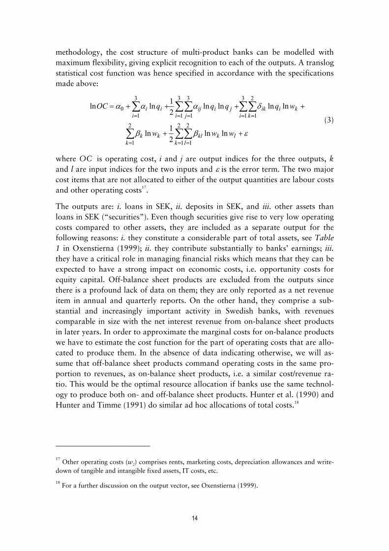
methodology, the cost structure of multi-product banks can be modelled withmaximum flexibility, giving explicit recognition to each of the outputs. A translogstatistical cost function was hence specified in accordance with the specificationsmade above:

���

����

��

�����

���

�����

� ��

� �� ��

2

1

2

1

2

1

3

1

2

1

3

1

3

1

3

10

lnln21ln

lnlnlnln21lnln

k llkkl

kkk

i kkiik

i jjiij

iii

www

wqqqqOC

(3)

where OC is operating cost, i and j are output indices for the three outputs, kand l are input indices for the two inputs and � is the error term. The two majorcost items that are not allocated to either of the output quantities are labour costsand other operating costs17.

The outputs are: i. loans in SEK, ii. deposits in SEK, and iii. other assets thanloans in SEK (“securities”). Even though securities give rise to very low operatingcosts compared to other assets, they are included as a separate output for thefollowing reasons: i. they constitute a considerable part of total assets, see Table1 in Oxenstierna (1999); ii. they contribute substantially to banks’ earnings; iii.they have a critical role in managing financial risks which means that they can beexpected to have a strong impact on economic costs, i.e. opportunity costs forequity capital. Off-balance sheet products are excluded from the outputs sincethere is a profound lack of data on them; they are only reported as a net revenueitem in annual and quarterly reports. On the other hand, they comprise a sub-stantial and increasingly important activity in Swedish banks, with revenuescomparable in size with the net interest revenue from on-balance sheet productsin later years. In order to approximate the marginal costs for on-balance productswe have to estimate the cost function for the part of operating costs that are allo-cated to produce them. In the absence of data indicating otherwise, we will as-sume that off-balance sheet products command operating costs in the same pro-portion to revenues, as on-balance sheet products, i.e. a similar cost/revenue ra-tio. This would be the optimal resource allocation if banks use the same technol-ogy to produce both on- and off-balance sheet products. Hunter et al. (1990) andHunter and Timme (1991) do similar ad hoc allocations of total costs.18

17

Other operating costs (w2) comprises rents, marketing costs, depreciation allowances and write-down of tangible and intangible fixed assets, IT costs, etc.

18 For a further discussion on the output vector, see Oxenstierna (1999).

15

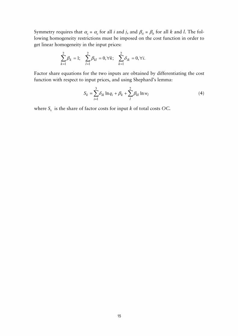
Symmetry requires that �ij = �ji for all i and j, and �kl = �lk for all k and l. The fol-lowing homogeneity restrictions must be imposed on the cost function in order toget linear homogeneity in the input prices:

.,0;,0;12

1

2

1

2

1ik

kik

lkl

kk ����� ���

���

���

Factor share equations for the two inputs are obtained by differentiating the costfunction with respect to input prices, and using Shephard’s lemma:

�� ���

�

23

1lnln

llklk

iiikk wqS ��� (4)

where Sk is the share of factor costs for input k of total costs OC.

16

The traditional statistical tests used for inference testing require the underlyingtime series to be stationary since regression with non-stationary time series cangive spurious results. Testing for stationarity was done with the augmentedDickey-Fuller (ADF) test. Results are reported in Table A2.1 from which it is evi-dent that all series are I(1). All series were therefore differenced once and thenbrought back to their mean levels.19

After adding an error term to (3) and attaching the share equations, the full dualsystem is estimated with the iterative seemingly unrelated regression (SUR) tech-nique. One of the share equations is omitted at the estimation since the system ofshare equations is singular because of the adding-up constraint, �Sk = 1. The es-timated parameters and their standard errors and t-statistics are given in TableA2.2. Goodness-of-fit measurements for the cost equations are in Table A2.3.Marginal operating costs are derived from (3):

��

�

�

��

�

����

��

�

23

1ln

kkik

jjiji

iii wq

qOC

qOCMOC ��� (5)

The calculated marginal operating costs based on the obtained parameter esti-mates are reported as averages over time in Table 1 and as time series in Figures 3– 6. For the loan market, the marginal costs are augmented with normalised op-erating costs for ex ante loan losses from new loans, and with opportunity costsfor equity capital, in accordance with the specifications made above. The methodsof estimating these items are worked out in Oxenstierna (1999). Since that essayuses the same data set as this one, the numerical values for these items are takenfrom there. As expected, the operating cost allocated to other assets (q3) is verylow.

19

As an alternative to the more simple technique of differencing, Berndt (1991, ch 9) proposes avector autoregressive process specification in the presence of autocorrelation. This involves apply-ing an autocovariance matrix to the cost function (4) as well as to the factor share equations (5).However, the singularity of the factor share system “imposes severe identificability and diagonalityconstraints on the autocovariance matrix” (p. 478), in essence that all equations in the whole sys-tem have the same lag coefficient for all lagged variables. Since this is “a very strong restriction”(op cit), I have refrained from using the VAR specification in this case.

17

A number of alternative estimations were also conducted to check the robustnessof the results. (1) Excluding the third output from the cost function influenced theensuing marginal cost estimates with less than plus 5% for the deposit marketand had a negligible effect on the loan market estimates. (2) Excluding the costshare equations from estimation influenced the ensuing marginal cost estimateswith between plus 5 to 10% for the two-output model, and with minus 5 to 10%for the three-output model. However, the significance of estimated parameterswas lowered.

Loan MOC,excl. pred.loan losses

PredictedMOC for

loan losses

MEC forequitycapital

MEC forloans;sum ofcol. 2-4

MEC fordeposits

MOC forother

assets

Bank 1 1.37 0.43 0.32 2.12 1.16 0.009Bank 2 2.20 0.47 0.32 2.99 1.30 0.037Bank 3 1.47 0.43 0.27 2.17 1.24 0.006Bank 4 1.98 0.50 0.24 2.72 1.54 0.045Bank 5 1.71 0.22 0.32 2.25 1.33 0.060

Table 1. Marginal costs reported as yearly averages over time in percent of the amount of totalloans, total deposits, and other assets, respectively. MOC = marginal operating cost, MEC =marginal economic cost. Values in columns 2, 6 and 7 are calculated from (5) using the esti-mated parameter values from (3) and (4). Values in columns 3 and 4 are estimated in Oxen-stierna (1999).

3.2.3 Estimating demand equations. Determining market parameters.

The first stage is to estimate the market demand equations for the two markets,loans and deposits.20 The resulting estimates will allow us to determine the mar-ket equation parameters � and � for each of the markets.

When estimating loan demand and deposit liability demand functions from timeseries, we again test for stationarity of all variables with the ADF test. Resultsare reported in Table A2.1, from which it is evident that all series are I(1). Addi-tionally, pM and other series included in the estimates below are also all I(1).

20

It should be noted, that I estimate demand equations and not demand elasticities. The reason isthat time series data will yield time-dependent, unstable values for structural parameters if the pa-rameter estimates from linear demand equations are used first to calculate elasticities and then todeduct parameter values for the theoretical model. The only alternative would be to estimate aconstant elasticity function, but that would presuppose a specific functional form for market de-mand, which is not compatible with the linear form of the market demand equations (1) and (2).

18

Economic theory tells us that quantity is the dependent variable in the marketdemand relationship. This assumption was tested with the Granger causality test.For both the loan market and the deposit market, results are that we can rejectthe null hypothesis that the price does not Granger cause the market quantity. Weare also unable to reject the reverse null hypothesis, that the market quantity doesnot Granger cause the market price, on the 5 per cent level of significance (F -test)for both markets.21 Since it is clear from both economic theory and from theseGranger causality tests that quantities are the dependent variables in both mar-kets, I will follow the Engle and Granger (1987) two step method in order to es-tablish co-integrating vectors and error correction mechanisms (ECM).22

Economic theory, and the model used here, defines the demand function as hav-ing quantity as the dependent variable and own-price as one of the independentvariables. Apart from that, there is no theoretical prescription on how a single-market demand function might be constituted, for what reason it seems advisableto apply a “general to specific” modelling approach.23 The general model is in anautoregressive distributed lag (ADL) form, where the dependent variable is afunction of its own lagged values and the contemporary and lagged values of allexplanatory variables. For a generalised demand function, we get the followingADL(m,n:k) formula, where m,n are the numbers of lags, k is the number of ex-ogenous variables and the error term ut � IID(0, �2):

uxqqm

i

k

j

n

iitjjiitit � ��

� � �

������

1 1 0,0 ��� (6)

3.2.3.1 Estimation technique and results

In the current setting, the theoretical model in Oxenstierna (1998) defines fourdifferent equilibrium price equations (supply relationships), but does not provideany obvious link between them that can be used in the estimation. There is on theother hand no need to make a systems estimation of the demand equation and the

21

The tests were made with one lag for the deposit market and four lags for the loan market.There are 33 observations and the F statistics are 3.77 for the loan market and 7.13 for the depositmarket.

22 An alternative would be the more demanding Johansen (1989) method, built on the vector auto-

regressive (VAR) methodology, primarily designed for problems where there are no a priori exoge-nous variables.

23 The general to specific modelling is proceeding from a fairly unrestricted dynamic model, which

is subsequently tested and reduced in size by testing different restrictions, see Charemza andDeadman (1997).

19

price equation simultaneously, since all parameters that are needed to feed thetheoretical model are defined either in the demand equation or in the exogenouslydetermined cost equation.24

Demand parameters can be consistently estimated in the presence of unobserveddemand factors via the use of traditional instrumental variables methods, such asthe two stage least squares method (TSLS), or the generalised method of moments(GMM). Correlation between the price variable and the error term suggests theuse of instruments for prices, assuming that the demand error is uncorrelatedwith the instrument. Demand is specified to have a nonzero disturbance, which isassociated with unobserved determinants of demand that are correlated acrossconsumers in the market. If these disturbances are known to the suppliers and theconsumers (and if demand depends upon them, one expects this to be so), thenequilibrium quantities and prices will depend upon the disturbances. The simul-taneity problem and the need for alternatives to ordinary least squares estimationtechniques arises from this relationship between the disturbance and price.

Predetermined (i.e. exogenous and lagged endogenous) variables and cost func-tion variables are thus used as supply-shifting instruments for endogenous pricesin order to identify demand. Additionally, it seems relevant to take into consid-eration the possibility that the market conduct has been changing during thesample period, since spread levels have displayed a specific pattern over time, cf.Fig 1. In order to control for this, I have added a Lerner index, lagged one pe-riod, as a proxy for changes in the market conduct, to the list of instrument vari-ables.25

The loan market ADL structure was tested with m, n = 5 and the following ex-tensive range of candidates for exogenous variables: the own-price (pL, which isnet of the money market rate), the deposit market net interest rate, the short-termmoney market rate (pM), the bond market rate for 5-year government bonds (pobl),the GDP (Y ), the stock market index, the consumer price index, and household

24

However, it might be possible to estimate a simple mark-up supply relationship simultaneouslywith the demand equation, in order to improve the significance of demand parameter estimates.But since estimates obtained from estimating the demand equations separately are highly signifi-cant for all 12 equations, this has been deemed not necessary.

25 The Lerner index is defined as (p – MC)/p. All estimations were also executed without the lagged

Lerner index as instrument variable. Results were not much influenced: The value of the estimatedprice parameter declined with 2% for the loan market and increased with 3% for the deposit mar-ket. Another attempt to control for changes in conduct was made by including a market concen-tration variable (CR5) as an instrument variable. This had a negligible effect on the estimates. Alsothe level of credit losses were tried as an instrument variable, the idea being that non-normal creditlosses during the banking crisis would influence conduct. Also this had a negligible effect on theestimates.

20

debts as a percentage of disposable income (Z). The latter variable captures thefact that households lowered their debt levels from around 140% debt to dispos-able income in 1989, down to 85% in 1996, i.e. a deep change of preferences forhaving debt. The lowered household debt levels during the 1990s are due to someabstruse structural changes taking place in the early 1990’s (see Berg, 1997), withi. a tax reform that together with other factors raised loan rates after tax with caseven percentage points from 1990 to 1995, ii. a “credit crunch” during thebanking crisis in 1991–3, iii. worsened economic outlooks for households, and iv.demographical changes. The stock of household debt thus diminished from 990billion SEK in 1989 to 730 billion SEK in 1996.26 The debt level was in 1997back at the ratio it had before the great expansion of credits commencing in themiddle of the 1980’s.

Non-financial firms also show a declining trend of bank loans as a proportion oftheir total debt, from around 39% in 1989 to around 29% in 1997. This trendlargely reflects the “credit crunch” during the banking crisis, including write-offsof bad debt. The decline entirely affects the credit lines to corporations, whereasfixed amount loans display a stable growth. There is a steady trend in banks’loan portfolios towards more of corporate loans (from 20% of total loans in1989 to 45% in 1997), whereas corporate credits are declining somewhat (from15% of total loans in 1989 to 11% in 1997). Nedersjö (1995) notes that largecredit-worthy corporations increasingly have raised financial capital directly onthe financial markets, leaving banks with a larger share of comparatively smallerand possibly riskier corporations in their loan portfolios. She suggests that thiscould explain the increasing (loan) interest rate spread from 1989-1994, sincecorporate credits command a somewhat higher interest rate than corporate loans.However, there are no data available on the size distribution of banks’ corporateloan portfolios. The interest rate spread is also on the same level in 1997 as it wasin 1989, see Fig. 1. I conclude that it is unlikely that structural changes in banks’corporate loan portfolios are an important factor in explaining the loan pricingconduct during the sampling period.

Estimation was done with TSLS on variables in levels. Predetermined variableswere included based on the analysis of variance (ANOVA) technique. The fol-lowing ADL structure resulted, with all parameters being significant on the 1%level, except pobl, which is significant on the 5% level (with t -statistics in paren-theses):

26

Data for this and for the household savings ratio used in the deposit equation below were ob-tained from Nationalräkenskaperna and Finansräkenskaperna. A thorough statistical andeconometrical analysis of these trends is found in Berg (1997).

21

)48.5()22.8()18.2()75.5()84.6()45.5(5.3211.738.24.25553.0226 2

��

������� t

Mt

oblt

Lttt ZpppLL

(7)

R2=0.92, R2

adj = 0.91, DW = 1.77

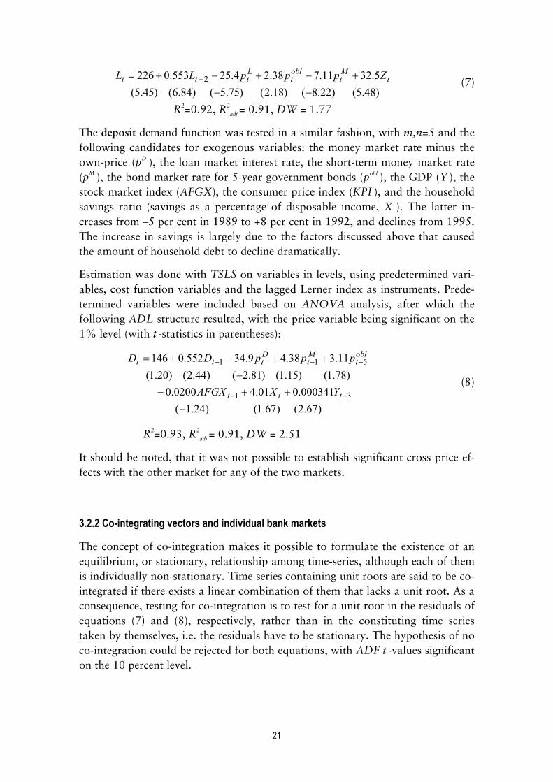
The deposit demand function was tested in a similar fashion, with m,n=5 and thefollowing candidates for exogenous variables: the money market rate minus theown-price (pD ), the loan market interest rate, the short-term money market rate(pM ), the bond market rate for 5-year government bonds (pobl ), the GDP (Y ), thestock market index (AFGX), the consumer price index (KPI ), and the householdsavings ratio (savings as a percentage of disposable income, X ). The latter in-creases from –5 per cent in 1989 to +8 per cent in 1992, and declines from 1995.The increase in savings is largely due to the factors discussed above that causedthe amount of household debt to decline dramatically.

Estimation was done with TSLS on variables in levels, using predetermined vari-ables, cost function variables and the lagged Lerner index as instruments. Prede-termined variables were included based on ANOVA analysis, after which thefollowing ADL structure resulted, with the price variable being significant on the1% level (with t -statistics in parentheses):

)67.2()67.1()24.1(000341.001.40200.0

)78.1()15.1()81.2()44.2()20.1(11.338.49.34552.0146

31

511

�

���

�

�����

��

���

ttt

oblt

Mt

Dttt

YXAFGX

pppDD

(8)

R2=0.93, R2

adj = 0.91, DW = 2.51

It should be noted, that it was not possible to establish significant cross price ef-fects with the other market for any of the two markets.

3.2.2 Co-integrating vectors and individual bank markets

The concept of co-integration makes it possible to formulate the existence of anequilibrium, or stationary, relationship among time-series, although each of themis individually non-stationary. Time series containing unit roots are said to be co-integrated if there exists a linear combination of them that lacks a unit root. As aconsequence, testing for co-integration is to test for a unit root in the residuals ofequations (7) and (8), respectively, rather than in the constituting time seriestaken by themselves, i.e. the residuals have to be stationary. The hypothesis of noco-integration could be rejected for both equations, with ADF t -values significanton the 10 percent level.

22

The co-integrating vector for each of the two equations can now be calculated bytaking expectations of all variables, which is the same as equating each variablewith all of its lags.27 The long run coefficients can then be calculated from the es-timated coefficients, see Banerjee et al. (1993, Ch 2). The resulting co-integratingvectors are, for the loan market:

ZpppL MoblL 6.729.1532.57.56505 ����� (9)

and for the deposit market:

D = 326 – 77.8 pD + 9.77 pM + 6.93 pobl (10)

+ 8.92 X – 0.0446 AFGX + 0.000761Y

The co-integrating vectors (9) and (10) directly yield the market parameters � and� for each of the two markets, respectively. The next step is therefore to deter-mine the product differentiation parameters �i. These are established in the sameway as for the aggregated markets; by estimating ADL equations with instrumen-tal variables’ techniques, and calculating co-integrating vectors for individualbanks. The resulting equations and co-integrating vectors are reported in Appen-dix 2. Again, it was not possible to establish significant cross price effects be-tween any of the banks and individual competitors. The reason for this is evi-dently that the weighted average cross price effect (which was always included inthe estimations due to the way the market model (1) is defined) uniformly domi-nates individual cross price effects between bank i and any bank j.

In order to empirically deduct the �i parameters, we first need to rewrite the esti-mated co-integrating vectors. These are in the form (see Appendix 2):

ij

k

jijiiiii uxppL ����� �

�3210

ˆˆˆˆ ���� , which translates into:

� � � � ij

k

jijiiiiiii uxpppL ������� �

�32210

ˆˆˆˆˆ ����� (11)

We note that we can rewrite (1) as a statistical function on the following form:

27

The Granger representation theorem (Engle and Granger, 1987) proves that a co-integrated sys-tem of variables can be represented in three isomorphic forms: the VAR, the ECM, and the mov-ing-average forms. Here we are pursuing the first step in their two-step procedure, where the pa-rameters of the co-integrating vector are estimated by running the TSLS regression in the levels ofthe variables. In the second step, the obtained parameters are used in the ECM form, see section3.2.6. Phillips and Loretan (1991) show that there are several alternatives how to estimate the longrun relationship, one of them the ADL approach used here. An ECM is simply a linear transforma-tion of the ADL, see Banerjee et al. (1990) and Banerjee et al. (1993).

23

� �ppspssL iiiiiii ���� ���� ˆˆˆˆˆˆ + �i, (12)

where ij

k

jiji ux �� �

�3�� . The size parameters, is , which are considered to be ex-

ogenous in the short run, are in this case determined by direct observation oflagged market shares. We can then solve for the �i values in (12) by equating thecorresponding factors from (11) and (12): 2

ˆˆˆ iiis ��� � . This procedure yields �i

parameters that are time-stable except for the influence from si.28

Loans,calculated pa-

rameters

Deposits,calculated pa-

rameters

Loanelasticities,

averages overtime

Depositelasticities,

averages overtime

Market � = 505� = 56.7

� = 326� = 77.8 -0.40 -0.51

Bank 1 �1 = 2.4(0.27)

�1 = 2.2(0.13)

-0.90(0.20)

-1.2(0.46)

Bank 2 �2 = 2.3(0.25)

�2 = 0.91(0.046)

-1.2(0.32)

-0.88(0.22)

Bank 3 �3 = 2.2(0.31)

�3 = 0.89(0.078)

-1.2(0.34)

-0.86(0.28)

Bank 4 �4 = 1.6(0.19)

�4 = 1.5(0.079)

-0.87(0.21)

-1.0(0.26)

Bank 5 �5 = 1.2(0.090)

�5 = 1.7(0.050)

-1.1(0.29)

-1.3(0.31)

Table 2. Calculated market parameters for the two aggregated markets, and the individualbanks. Deposit elasticities are transformed into demand elasticities since they are estimated netof the money market rate. Elasticities and �i values are averages for the sample period, 89:1-97:2. Standard deviations in parentheses.

As an additional check, long run market elasticities are calculated from the co-integrating vectors (9) and (10). For individual bank markets, the own price elas-ticity is deducted from (1):

� �� �iiii

iii ss

Lp

���� 11 ��� , (13)

28

In comparison, the alternative method where parameter values would be determined from elas-ticities, yields less stable values since elasticities have higher standard deviations over time, (e.g.,the �i values would vary not only with si but also with the ratio Li /pi if they were deducted from(13)). See footnote 20.

24

and is calculated by insertion of the estimated parameters, see Table 2.29

Elasticity measures are bound to be imprecise and to vary between different speci-fications.30 Elasticities are in reality a function of time, so that, a priori, a longerinterval between observations has a higher elasticity.31

3.2.4 Calculation of the theoretical equilibria

With all market parameters determined, see Table 2, the next task is to evaluatewhich of the different game-theoretical equilibria (see Oxenstierna (1998), ex-pressions (13), (16) or (18)) for each of the two markets, that best conforms tothe actual behaviour of each bank. The needed inputs are the calculated parame-ter values, �, �, �i, si and the average costs (which are equal to marginal costs dueto the assumption of short-term (within the period) constant returns to scale).Computations are done for each bank in each quarter. Results are reported inFigures 3 - 4 for the loan market, and in Figures 5 - 6 for the deposit market.This is a positive analysis, where observed prices are gauging the explanatorypower of the different theoretical market regimes, as represented by the variouscalculated equilibrium prices, ranging from marginal economic cost pricing tomonopoly pricing.

29

To my knowledge, there are no prior estimates of bank market elasticities on Swedish data. Theelasticities are of the same magnitude as internationally reported elasticities. Berg and Kim (1998)report the following disaggregate loan market elasticities for Norwegian banks for the period1988-91: Retail loans: -0.90; corporate loans: -0.86. No elasticities are reported for individualbanks. Vesala (1995) reports the following elasticities from Finnish bank markets: Loan marketdemand elasticity: -0.55. Individual banks’ own demand elasticities range from -1.45 to -4.14. De-posit market supply elasticity: 0.17. Individual banks own supply elasticities range from: 0.28 to0.61.

30 Edgerton et al. (1996, ch 6) study imprecision in elasticity estimates due to specification error

(structural variation) by comparing the results from non-dynamic and dynamic versions of thesame type of model applied on the same time series data set. They find that the model choice leadsto big and statistically significant effects, where differences are in excess of the model consistentvariations for nearly all goods estimated. This raises doubt on previous bank market studies thathave not taken the time structure of bank markets into explicit consideration. Only one previousstudy is known to have done so, Swank (1995).

31 This is also what Assarsson (1996) finds when estimating elasticities for different goods and

services on Scandinavian countries’ household data, using an ECM variant of a dynamic almostideal demand system. The precision of estimated elasticity is also substantially influenced by thechoice of model, and by the choice of estimation method. All these sources of variations causeEdgerton (op. cit. p 166) to conclude that, in general, an interval of �0.25 is the minimum level ofuncertainty of elasticity measures on individual Swedish consumption goods.

25

3.2.5 Evaluating the conduct in the markets

Because of the large amount of data, I will evaluate conduct mainly from in-specting the figures. Starting with the overall markets (Fig 1, which summarisesevents in the two markets by adding their observed prices, their estimated costsand their theoretically deducted prices, respectively), it is evident from thegraphed total spread compared to the total economic costs, that the Swedishbanking markets have gone through a period of less competitive conduct. The to-tal spread at the beginning of 1989 of about 5% increased to about 6.5% in1992-93, but has since then sunk back to about 4.7% in the beginning of 1997,whereas costs have been fairly constant throughout the period. The major expla-nation for the increase in spread is most likely to be the profound banking crisisin Sweden, which gave banks an opportunity to exercise their market power. Thebanking crisis, which had its main impact during 1991-3, was mainly a propertylending credit risk phenomenon, but, evidently, deposit customers had to pay themajor part of the price for it, since the overall increase in spread was due mainlyto an increased spread on the deposit market during the crisis, (compare Fig. 3and Fig. 5). Apparently, market power was greater on the deposit side during thatperiod. Also, there was a profound shift of propensities to loan and to save dur-ing the period so that households and firms lowered their debt levels substantiallyby saving for amortising (Berg, 1997). This changed banks from being “asset-driven” to being “liability-driven” (Matten 1996), i.e. they got large excess de-posit volumes. These were difficult to place at the higher margins that private sec-tor loans command, which in turn might have had a negative impact on the de-gree of competition in the deposit market.

In order to analyse the market conduct in more detail, I have divided the sam-pling period into five sub-periods, see Figures 3, 5, 7 and 8. During the first pe-riod, which is the “pre-crisis” period, 89:1 – 91:1, spreads are increasing in thedeposit market and declining in the loan market. The probable reason for this isthat banks faced a strong decline in loan demand, see Fig. 8, which causes compe-tition to increase. The decline in loan demand is caused by a combination of low-ered household and corporate debt levels and an increase in households’ savingsratio from –5% of disposable incomes in 88:4 to around zero in 91:1 (StatisticsSweden, BNP/kvartal). The increase in savings does, however, not turn up asbank deposits, but is evidently used to amortise bank loans (Fig. 8). It is thereforedifficult to explain the big increase in deposit spread (+0.7 percentage points)during the pre-crisis period with exogenous factors. One hypothesis is that banksshifted their market power from the loan market, where competition was in-creasing due to a declining demand, to the deposit market, where demand wasconstant in real terms. As regards the interest rate levels, see Fig. 5, they are bestexplained by the hypothesis of Nash equilibrium with respect to quantities(henceforth called NE(q)) for deposits in 89:1, increasing above the monopoly

26

price level in 91:1. The loan market rates, on the other hand, declined down tothe marginal economic cost (MEC) level in 91:1, see Fig. 3.

The second period represents the deep banking crisis from 91:2 – 92:4. Duringthis period the exogenous trends of changing savings and loans behaviour con-tinue, making banks increasingly liability-driven. Together with large write-offsof bad debts, this gives banks excess deposits of around 50 Bn SEK. Since excessdeposits have to be placed at lower interest rates than commercial loans, there is adis-incentive for competition for deposits, which is the likely explanation for theincreased spread in the deposit market with another 0.5 percentage point. In thesecond half of this period, however, the strong increase in demand for deposit li-abilities abate (Fig. 8), and the spread level stabilises (Fig. 5) above the monopolyprice. This high price level can be explained by the fact that banks got large vol-umes of excess deposits (Fig. 7), so that they became increasingly liability-drivenand less competitive in their pricing of deposit services. In the loan market, thereis a continued strong decline in loan demand, which keeps pricing competitiveand prices are kept down to near the economic cost level (Fig. 3). Economic costlevels are stable in each of the two markets throughout both the first two periods.

The third period, 93:1 – 94:2 depicts the resolution of the banking crisis.32 Thesavings quota is now stabilised at a record high of around 8% of disposable in-come. Loan demand measured as loan stocks related to household disposable in-come continue to decline down to 1.5 in 94:2 (from 2.5 at its peak in 1989). Thebulk of bad debt write-offs also occurred during this period, so that overall loandemand dropped dramatically, see Fig. 8. These factors taken together meant thatbanks built up excess deposits on the level of 150 Bn SEK, see Fig. 7. Depositspread drops from 4.1% down to 2.3%, which is close to the NE(q) level. Thiscan to a minor part be explained by the continued decline in economic costs onthe deposit side, see Fig. 5. On the other hand, loan economic costs increase dueto rising equity costs, see Fig. 3, which is part of the explanation for the quicklyincreasing loan rates, from the MEC level in 92:1, up towards the level corre-sponding to the Nash equilibrium with respect to competition in prices (hence-forth NE(p)) in 93:4. However, the dramatic shifts in market power betweenmarkets should mainly be understood as a short-term adjustment, as will be elu-cidated in the next section.

The fourth period, 94:3 – 96:1, is a revival period for the loan markets. Finally,loan demand picks up and the savings ratio starts to drop, which together make

32

Already in mid-1993 the large banks and the stock market felt that the crisis was contained. Forexample, S-E-Banken’s shares reached their pre-crisis level in August 1993, and a new emission ofstocks doubling the share capital was successfully placed. Also Handelsbanken and Swedbankmade big emissions of new stocks at the same time.

27

excess deposits decline somewhat, see Figures 7 and 8. Loan spread decreasesdown to the marginal economic cost level (Fig. 3), without any plausible exoge-nous explanation, except that the increase in period III was a short-term adaptivephenomenon which is slowly corrected in period IV (see the next section for afurther elaboration of this). One possible endogenous explanation might be thatbanks started to compete for loan market shares again after surviving the crisis.Also, a number of small new low-cost banks were established during this period,which influenced the competitiveness of the retail markets, mainly the depositmarket. In the deposit market, spreads are again increasing, from the NE(q) levelto the monopoly price level, (Fig. 5). This is particularly noticeable since marginalcosts for providing deposit liability services are declining rapidly.

In the fifth period, 96:2 – 97:2, there is a return to the familiar pattern from pe-riod III. The savings ratio continues to drop, which, together with the ever in-creased competition from newly established niche banks, might explain the sig-nificant drop of the deposit spread to below the NE(p) level, (Fig. 5). There is,however, a mirror-imaged pattern in the loan market. Loan demand continues togrow (Figures 7 - 8), and banks are able to raise the loan spread from the MEClevel halfway up towards the NE(p) level, (Fig. 3). Also in this period, there is astrong decline in market interest rates, with three percentage points, (See Fig. 3 inOxenstierna (1999)). The alternative hypotheses proposed and tested with theECM estimations in the next section explains the conduct in periods III and Vprimarily as short-term adjustments.

The overall picture of bank conduct during all the five periods in both markets, isthat the economic cost level constitutes a bottom level for pricing policies, andthat attempts to establish higher spreads are not sustainable in the long run in theloan market. In the deposit market, the huge amounts of excess deposits givessmall incentives for price competition, so that average spreads over the entire pe-riod are best explained by the hypothesis of monopoly pricing.

3.2.6 Transmission of money market rates into loan and deposit rates

One important monetary policy issue with regard to the relation between moneymarket interest rates and the banking markets, is how efficiently the money mar-ket rates are passed through to the loan and deposit market rates. These twomarkets display price stickiness, as evidenced primarily through periods III to V,when the relative spread levels between the markets are distorted due to rapidlyfalling money market rates, see Fig. 2, 3 and 5. For these reasons it is of some in-terest to investigate the patterns of price stickiness.

Price stickiness can be explained by menu costs arising from the activity ofchanging prices, as in Rotemberg and Saloner (1987) or, in a banking applica-

28

tion, in Hannan and Berger (1991). They explain the often observed phenomenonof greater price rigidity in a monopoly than in an oligopoly, by a proposition thathigher price elasticities increases the incentives to alter prices in response tochanging marginal costs. In this case, the Swedish banking markets should beequally sticky, since elasticities are of the same size in both markets. But as will bedemonstrated below, the loan market is significantly more sticky than the depositmarket, which calls for other explanations than menu costs.

By carrying out ECM estimations, some further light can be shed on the issue ofshort-term adjustments. Following Bårdsen (1989), we can hence rewrite theADL in (6) as an ECM, without imposing any restrictions on the model:

t

m

i

k

j

n

imitjjiitit uECTxyy � ��

�

� �

�

�

�������

1

1 1

1

0

*,

**0 ���� ��� , (14)

where ��

��

m

iim

1

* 1�� , ��

�

n

ijijn

0

* �� and where the error correction term (ECT j )

for the jth equation is defined as:

��

����

k

jntjjmt

j xyECT1

,� , with *

*

m

jnj

�

��

�

� .

For the loan market we obtain:

tMt

oblt

Ltt

L ZpppLECT 6.729.1532.57.562 ������

and for the deposit market:

31

511

000761.092.80446.093.677.98.77

��

���

���

����

ttt

oblt

Mt

Dtt

D

YXAFGXpppDECT

The ECT series were then tested for stationarity with the ADF test. The hypothe-sis of stationarity could not be rejected for any of the two series, on the 5% levelfor ECT L and on the 1% level for ECT D, i.e. all elements of the ECMs are I(0).The ECMs (14) are then estimated with OLS, yielding the following results forthe loan market (with t -statistics in parentheses):

)51.2()55.6()36.0()021.0()72.0()68.2(

104.02.65617.00262.072.30.55

���

������LMoblL ECTZpppL �����

(15)

R2 = 0.75, R2

adj = 0.70, DW = 2.23

For the deposit market we get:

29

)15.4()25.0()47.0(484.000525.006.2

)02.2()50.0()53.0()08.2()38.4(

000206.014.145.13.23161

���

��

��

������

D

oblMD

ECTAFGXX

GDPpppD

��

�����

(16)

R2 = 0.64, R2

adj = 0.50, DW = 2.19

As expected, the ECT parameters are negative. The ECT parameter also has aneconomic interpretation: In general, it measures a variable’s speed of adjustmentback to the equilibrium level (Johansen (1989, p 16), quoted in Charemza andDeadman (1997)) which in this case is the number of quarters it takes to returnto the long-run equilibrium after the occurrence of a disturbance. Thus it givescompleting information on short-run behaviour. For the loan market the value isalmost 10 quarters and for the deposit market it is about 2 quarters. The differ-ence between the two markets indicates that banks’ loan stocks are slower toadapt to changing market interest rate conditions than deposit stocks.

One important factor in both periods III andV is that money market rate levelsdropped significantly, see Fig. 2. Since loan stocks and deposit stocks are likely toadapt with different speeds to dramatic shifts in interest rate levels, this could alsoexplain the shift in net spreads between the two markets as a short-term dynamicphenomenon. Rapidly falling loan interest rates induce some customers withfixed interest rate loans to renegotiate their loans. When interest rates go down,not all loans are renegotiated, so that banks continue to earn the high rates onnot renegotiated loans, causing net loan spread to increase.33 Similarly, some partof the deposit stock is fixed rate, so that banks will continue to pay high interestrates on such deposits, causing net deposit spread to decrease. Another factor thatis likely to influence these short-term adaptations is the slope of the yield curve,which was negative during the third period, see Fig. 2. and tilts throughout peri-ods III – V. As far as loan rates follow long-term market rates instead of the as-sumed short-term rates, the transmission of money market rates will not be com-plete. Banks can also absorb changes in money market rates when they determinetheir own reference rates (pM). However, the impression is that there has been anincrease over time in the usage of short-term rates as reference rates in lending,which would facilitate an improved pass-through of the market rates.

The pattern of dramatic shifts in observed price conduct between the two marketsin periods III through V (Figures 3 – 6) seems to support the proposition madeabove, that it mainly should be understood as a short-term phenomenon due to

33

When a customer renegotiates or cancels a fixed interest loan, a one-time compounded interestincome effect for the bank occurs. Such effects are not recorded in the Riksbank loan interest ratestatistics, since it registers the current rates on all loans.

30

differing adjustment speeds in the stocks of loans and the stocks of deposits, re-spectively. The greatly increased spread on loans in these two periods (Fig. 3)must therefore be seen in conjunction with the corresponding reduction in spreadon deposits (Fig. 5), with overall spread declining in both periods (Fig. 1). Theredistribution of spreads between the two markets thus seems to be mainly a ficti-tious phenomenon related to short-term adjustments in a volatile money marketinterest rate environment.

3.2.7 Evaluating the conduct of individual banks

It is possible to evaluate the conduct also of individual banks over time, and tocompare them in terms of cost levels, pricing strategies, development of marketshares, etc. However, such an evaluation would inevitably provide the means forrevealing the identity of the individual banks. Therefore, due to the secrecy of theRiksbank data set (cf. footnote 9), observations on the conduct of individualbanks will here be restricted to looking at only one sample bank in each market.Starting with the sample bank in the loan market in Fig. 4, we see a bank that hashigher economic costs than the average throughout the period. Further, it has aslightly more aggressive pricing policy than average until 95:2, after which itsprices are on par with the average. The pricing policy until 95:2 was not re-warded with increasing market shares, which are on the same level at the end of1994 as in 1989 (the dip in market shares during 92:2 – 93:3 might be due to re-porting irregularities during the banking crisis). From the beginning of 1995 thisbank has falling market shares, which, at least in part, might be attributable tothe change in pricing policy.

Turning to the sample bank in the deposit market (Fig. 6), this bank has a costlevel development that is very close to the average bank throughout the period.Until 92:3 it has a higher price level than average, and faces a slow decline inmarket shares. From 92:4 it changes to a more aggressive pricing policy and re-stores the market share in 93:4. In 1994, it switches back to its previous, less ag-gressive pricing policy with interest rates ca 0.3% above the average, and starts tolose market shares again.

All five banks display similar patterns of conduct as the sample bank. There areno real outliers, as evidenced by the estimated costs and elasticities in Tables 1 –2.

31

3.2.8 Evaluating the performance in the markets

Performance is evaluated by inserting observed prices, estimated costs and marketparameters into equation (37) in Oxenstierna (1998) for each quarter and eachmarket. This yields a measure of the welfare loss from non-competitive pricing. InTable 3, the calculated yearly averages are disclosed for each of the two marketsas well as totals.

Loans Deposits Total % of GDP1989 1339 10649 11987 1.0%

1990 1706 16646 18352 1.3%

1991 1528 17318 18846 1.3%

1992 2337 25751 28088 1.9%

1993 5352 13551 18903 1.3%

1994 4555 6888 11443 0.7%

1995 2312 11482 13794 0.8%

1996 4150 5443 9593 0.6%

Table 3. Calculated welfare losses from non-competitive pricing in Swedish bank markets. Values inSEK millions.

The welfare losses as a percent of GDP increase from about one percent in 1989up to almost two percent in 1992, adding to the accounting costs of the bankingcrisis. Welfare losses are then declining, and continue to do so in 1997. The aver-age welfare loss to society over the period 1989 – 1996 was 1.1% of GDP. Theconclusion above, regarding the shift of market power between markets, is againconfirmed. The deposit market is comparatively less competitive through 1995 asa combined effect of strongly increasing demand for deposit liabilities and a lackof competition during the banking crisis. From 1996, the picture is reversed, withincreasing demand for loans and increasing competition for deposits, togethershifting the bulk of welfare losses over to the loan market. However, this changeis, again, likely to reflect a short-term adaptation in stocks of deposits and loansto rapidly declining market interest rates, as elucidated in section 3.2.6. Overall,the deposit market has much larger welfare losses than the loan market.

4 Conclusions

In this essay an asymmetric oligopoly model for multi-product banking is devel-oped, based on the possibility to separate a bank’s activities in the deposit andloan markets. This requires absence of economies of scope and that there are no

32

demand interrelationships between the markets. These assumptions correspondwith empirical evidence on the Swedish banking markets. As an alternative to theprevailing conjectural variations models in Cournot competition, the full-fledgedgame-theoretic model with two types of product differentiation from Oxenstierna(1998) is employed to represent the market structures. This model’s range of dif-ferent game-theoretic equilibria are then used in a positive analysis, where ob-served prices are gauging the explanatory power of the different theoretical mod-els. Furthermore, the model allows for an evaluation of welfare effects, based onthe calculation of consumer surpluses. Any deviation from efficient pricing isevaluated on the individual bank level.

It appears that the model developed in Oxenstierna (1998) is well suited for anempirical analysis. The "structural richness" of the theoretical model simplifiesthe econometric work, due to the method developed for empirical application ofthe model, where the central econometric task consists of a straightforward esti-mation of demand equations: All market demand parameters for the n asymmet-ric banks are derived from estimating n bank-specific demand equations and anaggregated market demand for each market. Since all behavioural equations areprovided in the theoretical model, there is no need for empirical estimation ofbank-level conduct.

The model was applied to the Swedish banking oligopoly. Results show that thereis significant market power mainly in the deposit market, although with astrongly time-varying pattern. The loan market is found to be more competitive,but also displays strong time variations. In order to further analyse the short-termvolatility in conduct that is found, an error correction mechanism is deducted andestimated. This reveals different short-term behaviour in the stocks of depositsand loans, respectively. This result sheds some light on the monetary transmissionmechanisms in the Swedish banking system, where evidence is found of signifi-cant stickiness mainly in the loan market. Overall, conduct is declining from theNE(p) level at the end of 1993, down towards the competitive price level at theend of the period, see Fig. 1.

Summing up events in the loan market (Fig. 3), net spread (p – pM – economiccosts) was rising from around zero in 1990/1 to a peak in the beginning of 1994,but banks were unable to compensate themselves for the increasing equity costs,causing net spread to fall back to zero in 1995, then increasing to about 0.75% atthe end of the period. Conduct is on average best explained by the hypothesis ofmarginal economic cost pricing on average for the whole period, although thepost crisis period (III ) offered spread levels approaching the NE(p) level. Theoverall picture of bank conduct during all the five periods in the loan market, isthat the economic cost level constitutes a bottom level for pricing policies, andthat attempts to establish higher spreads are not sustainable in the long run.

33

There were profound structural changes in savings behaviour during the sampleperiod, making banks increasingly liability-driven, which to a large extent ex-plains short-term changes in pricing levels. The influence of these structuralchanges are most evident in the deposit market (Fig. 5), where the average con-duct in the market is best explained by the hypothesis of NE(q) prices at the beginof the period, but rapidly increasing until 93:2 so that net prices (pM – p) areabove the monopoly price. Thereafter, net spread falls rapidly down to the NE(q)level at the end of 1993. It subsequently reverts to the monopoly price level untilthe end of 1995. After that, it starts to fall, so that it is below the NE(p) price in97:2. It is clear that the persistent large volumes of excess deposits (around 150Bn SEK from 1994 and onwards, Fig. 7) have a detrimental effect on the degreeof competition. Cost levels are increasing until the begin of 1994, and thereafterfalling, so that they are one percentage point lower in 97:2 than at the peak level.

It is also possible to follow the conduct and relative pricing strategies of individ-ual banks. Finally, welfare losses to the society from non-competitive pricingwere calculated. The average level throughout the period 1989 – 1996 corre-sponds to ca 1.1% of GDP, mainly stemming from the deposit market, althoughthere was a strong increase in welfare loss levels due to non-competitive pricingduring the banking crisis, peaking at almost two percent of GDP in 1992. Afterthat, welfare losses are persistently declining, and are less than one percent ofGDP in 1997.

34

Appendix 1Tables with results from estimations

Variable Market Bank 1 Bank 2 Bank 3 Bank4 Bank5w1, level 1.1 2.8† 1.1 1.4 1.5

w1, 1st difference 5.2** 6.0** 3.3** 3.3** 4.5**

w2, level 3.0 1.4 0.7 2.5 1.3w2, 1st difference 5.4** 5.0** 4.2** 4.2** 4.0**

C, level 1.9 0.26 1.3 1.1 0.45C, 1st difference 4.7** 6.4** 3.0** 3.6* 2.6*

pL, level 1.8 2.1 1.8 2.3 1.6 0.36pL, 1st difference 5.3** 5.9** 5.8** 6.4** 5.5** 4.8**

L, level 1.2 2.9 2.1 2.2 2.2 1.7L, 1st difference 6.9** 5.6** 7.5** 5.4** 6.1** 3.4**

pD, level 1.8 2.0 0.77 2.0 1.7 1.7pD, 1st difference 4.5** 4.6** 4.0** 5.4** 5.0** 4.6**

D, level 2.3 2.8 2.1 2.7 2.1 2.2D, 1st difference 5.9** 7.7** 4.7** 4.0** 7.3** 5.1**

Table A1.1 Augmented Dickey-Fuller (ADF) tests: Absolute t -ratios. L is loans, D is deposits, pi are therespective interest rates net of the (smoothed) 3-month money market rate. † , * and ** denotes signifi-cance at the 10%, 5% and 1%-levels respectively, based on MacKinnon critical values. A constant anda time trend have been included in the ADF regressions, if significant. All 1st differences are signifi-cant on the 1% level.

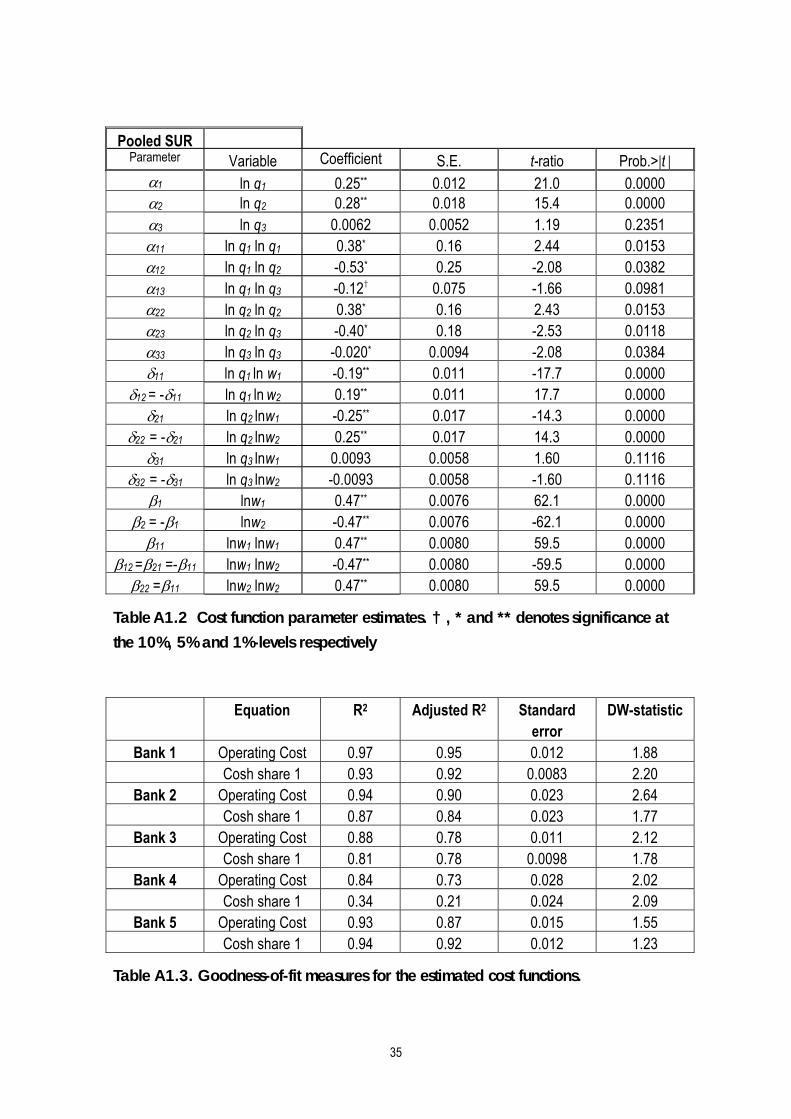
35

Pooled SURParameter Variable Coefficient S.E. t-ratio Prob.>�t �

�1 ln q1 0.25** 0.012 21.0 0.0000�2 ln q2 0.28** 0.018 15.4 0.0000�3 ln q3 0.0062 0.0052 1.19 0.2351�11 ln q1 ln q1 0.38* 0.16 2.44 0.0153�12 ln q1 ln q2 -0.53* 0.25 -2.08 0.0382�13 ln q1 ln q3 -0.12† 0.075 -1.66 0.0981�22 ln q2 ln q2 0.38* 0.16 2.43 0.0153�23 ln q2 ln q3 -0.40* 0.18 -2.53 0.0118�33 ln q3 ln q3 -0.020* 0.0094 -2.08 0.0384�11 ln q1 ln w1 -0.19** 0.011 -17.7 0.0000

�12 = -�11 ln q1 ln w2 0.19** 0.011 17.7 0.0000�21 ln q2 lnw1 -0.25** 0.017 -14.3 0.0000

�22 = -�21 ln q2 lnw2 0.25** 0.017 14.3 0.0000�31 ln q3 lnw1 0.0093 0.0058 1.60 0.1116

�32 = -�31 ln q3 lnw2 -0.0093 0.0058 -1.60 0.1116�1 lnw1 0.47** 0.0076 62.1 0.0000

�2 = -�1 lnw2 -0.47** 0.0076 -62.1 0.0000�11 lnw1 lnw1 0.47** 0.0080 59.5 0.0000

�12 =�21 =-�11 lnw1 lnw2 -0.47** 0.0080 -59.5 0.0000�22 =�11 lnw2 lnw2 0.47** 0.0080 59.5 0.0000

Table A1.2 Cost function parameter estimates. † , * and ** denotes significance atthe 10%, 5% and 1%-levels respectively

Equation R2 Adjusted R2 Standarderror

DW-statistic

Bank 1 Operating Cost 0.97 0.95 0.012 1.88Cosh share 1 0.93 0.92 0.0083 2.20

Bank 2 Operating Cost 0.94 0.90 0.023 2.64Cosh share 1 0.87 0.84 0.023 1.77

Bank 3 Operating Cost 0.88 0.78 0.011 2.12Cosh share 1 0.81 0.78 0.0098 1.78

Bank 4 Operating Cost 0.84 0.73 0.028 2.02Cosh share 1 0.34 0.21 0.024 2.09

Bank 5 Operating Cost 0.93 0.87 0.015 1.55Cosh share 1 0.94 0.92 0.012 1.23

Table A1.3. Goodness-of-fit measures for the estimated cost functions.

36

Appendix 2 Estimated ADL structures and co-integrating vectors for individual banks

Estimation was done with TSLS on variables in levels, using predetermined(i.e. exogenous and lagged endogenous) variables, cost function variablesand the lagged Lerner index as instruments (variable definitions are in sec-tion 3.2.3 except p bar, which is the weighted average market price). Prede-termined variables were included on the basis of the analysis of variance(ANOVA) technique. Specifically, it should be noted that none of the esti-mated equations had significant own-market cross-price parameters toother individual banks’ prices, but that all of them had significant parame-ters to the weighted average market price. In no case were across marketparameters significant, neither to other individual banks nor to the acrossmarket weighted average market price. The reason for this is evidently thatthe weighted average cross price effect (which was always included in theestimations due to the way the market model (1) is defined) uniformlydominates individual cross price effects between bank i and any bank j.

Individual loan markets

The following ADL structures resulted (t – statistics in parentheses), withgoodness-of-fit measures and calculated co-integrating vectors (CV) in theloan markets:

Bank 1

)55.1()30.1()70.1()29.6(0719.016.577.7819.0 41

�

������ t

Lt

Lttt KPIppLL

R2=0.85, R2

adj = 0.83, DW = 1.84

CV: KPIppL 396.04.288.42 ����

Bank 2

)15.1()93.2()04.3()91.1()21.2()66.2()78.3(9.43000119.0399.08.1209.98.10682.0 52311

���

������������ ttt

Lt

Lttt YKPIZppLL R2

=0.84, R2

adj = 0.80, DW = 2.17

CV: YKPIZppL 000374.025.13.406.280.34138 ������

37

Bank 3

)16.1()95.1()37.3(0000363.0104.079.1

)41.3()12.1()72.2()27.1()27.5(8.134.1209.444.9489.0

235

11

�

���

��

�����

���

��

ttoblt

tLt

Lt

Lttt

YKPIp

ZpppLL

R2=0.95, R2

adj = 0.94, DW = 2.21

CV: YKPIZpppL obl 0000710.0204.00.2750.32.245.26 �������

Bank 4

)39.1()05.1()2.11()62.1()07.1()01.2()00.7(8.190000257.05.219.1124.28.16497.0 222

��

���������� tt

Lt

Lt

Lttt YZpppLL

R2=0.97, R2

adj = 0.97, DW = 1.79

CV: YZppL 0000510.06.427.238.374.39 �����

Bank 5

)58.3()44.1()95.2()36.1()66.1()05.5(420.0295.00607.083.579.134.3769.0 411

��

����������

oblMttt

Lt

Lttt ppKPIZppLL R2

=0.95, R2

adj = 0.94, DW = 2.09

CV: oblM ppKPIZppL 82.128.1263.02.2575.75.14 �������

38

Individual deposit markets

The following ADL structures (t – statistics in parentheses) with goodness-of-fit measures and calculated co-integrating vectors (CV) resulted in thedeposit markets:

Bank 1

)61.1()88.3()63.1()42.1()38.1()39.1()42.1(2.330192.014.393.128.18.309.30 22111

�

�������������

AFGXppXppD Mt

obltt

Dt

Dtt

R2=0.93, R2

adj = 0.92, DW = 1.70

CV: 2.330192.014.393.128.18.309.30 �������� AFGXppXppD Moblt

Bank 2

)38.6()81.5()32.1()94.1()56.2()80.1(9.20654.247.11.276.36375.0 12

��

��������� t

Mt

Dt

Dttt XpppDD

R2=0.78, R2

adj = 0.73, DW = 1.81

CV: 15185.107.17.196.26 ������ XpppD Mt

Bank 3

)08.1()83.2()00.2()22.1()72.2()05.2(00490.0254.034.125.79.14392.0 33311

�

����������� tt

Mt

Dt

Dttt AFGXKPIpppDD R2=

0.92, R2

adj = 0.91, DW = 1.86

CV: KPIAFGXpppD Mt 417.000805.021.29.116.24 ������

Bank 4

)84.2()95.2()80.4()65.1()82.1()65.2(9.5804.137.14.173.17422.0 522

�

���������

obltt

Dt

Dttt pXppDD

R2=0.89, R2

adj = 0.86, DW = 2.45

CV: 10279.136.20.309.29 ������obl

t pXppD

Bank 5

)11.3()88.2()89.2()48.1()28.1()47.3(3.2000483.0669.035.826.7432.0 31221

�

����������� tt

Dt

Dttt AFGXXppDD R2=0

.92, R2

adj = 0.91, DW = 1.60

CV: 8.3500850.018.17.148.12 ������ AFGXXppDt

39

References

Assarsson, B., 1996, in Edgerton et al.: The Econometrics of Demand Systems.With Applications to Food Demand in the Nordic Countries, Kluwer Aca-demic Publishers

Banerjee, A., Galbraith, J.W. and Dolado, J.J., 1990, Dynamic Specification andLinear Transformations of the Autoregressive-Distributed Lag Model, Ox-ford Bulletin of Economics and Statistics, 52:1, 95-104

Banerjee, A., Dolado, J.J., Galbraith, J.W.,and Hendry, D.F., 1993, Co-integration, error correction, and the econometric analysis of non-stationarydata, Oxford University Press

Bårdsen, G., 1989, Estimation of Long Run Coefficients in Error CorrectionModels, Oxford Bulletin of Economics and Statistics, 51:2, 345-350

Berg, L., 1997, Hushållens skulder och förmögenhet – En analys av hushållensskuldsättning med utblick till år 2000, Nordbanken, Ekonomiska sekretariatet,Stockholm

Berg, S.A. and Kim, M., 1994, Oligopolistic Interdependence and the Structure ofProduction in Banking: An Empirical Evaluation, Journal of Money, Credit,and Banking, 26:2

Berg, S.A. and Kim, M., 1998, Banks as Multioutput Oligopolies: An EmpiricalEvaluation of the Retail and Corporate Banking Markets, Journal of Money,Credit, and Banking, 30:2

Bergendahl, Göran, 1989, The management of assets and liabilities in banks:Principles and applications, Revue de la Banque, 6/1989.

Berger, A.N., Hanweck, G.A., and Humphrey, D.B., 1987, Competitive Viabilityin Banking, Journal of Monetary Economics 20

Berger, A.N. and Humphrey, D.B., 1992, Measurement and Efficiency Issues inCommercial Banking, in Griliches, Zvi, (ed), Output Measurement in theServices Sectors, The University of Chicago Press, 1992.

Berger, A. N., Humphrey, D. B., and Pulley, L.B., 1996, Do consumers pay forone-stop banking? Evidence from an alternative revenue function, Journal ofBanking and Finance, 20, 1601-1621

Berger, A.N. and G. Udell, 1995, Relationship Lending and Lines of Credit inSmall Firm Finance, Journal of Business, 68, 351-382.

Berndt, E.R., 1991, The Practice of Econometrics: Classic and Contemporary,Addison-Wesley Publishing Company, Inc.

40

Berry, S.T., 1994, Estimating discrete-choice models of product differentiation,RAND Journal of Economics, 25:2, 242-262

Blomberg, Erik, 1994, Banking, in EEA and the Financial Services Sectors inSweden, Sveriges Riksbank Occasional Paper, 9.

Boyd, J. and E. Prescott, 1986, Financial Intermediary-coalitions, Journal of Eco-nomic Theory, 38, 211-232.

Bulow, J.I., Geanakoplos, J.D., and Klemperer, P.D., 1985, Multimarket Oligop-oly: Strategic Substitutes and Complements, Journal of Political Economy,93:3.

Charemza, W.W. and Deadman, D.F., 1997, New Directions in EconometricPractice. General to Specific Modelling, Cointegration and Vector Autore-gresseion, 2nd edition, Edward Elgar Publishing Ltd.

Christensen, L.R., D.E. Jorgenson and L.J. Lau, 1973, Transcendentallogarithmic production frontiers, Review of Economics and Statistics 55, 28-45.

Clark, Jeffrey A., 1996, Economic Cost, Scale Efficiency, and Competitive Vi-ability in Banking, Journal of Money, Credit, and Banking, 28:3, 342-364.

Diamond, D., 1984, Financial Intermediation and Delegated Monitoring, Reviewof Economic Studies, 51, 393-414.

Edgerton, D.L, B. Assarsson, A. Hummelmose, I.P. Laurila, K. Rickertsen, P.H.Vale, 1996, The Econometrics of Demand Systems. With Applications toFood Demand in the Nordic Countries, Kluwer Academic Publishers.

Englund, Peter, 1990, Financial Deregulation in Sweden, European Economic Re-view 34: 385-393.

Engle, R.F. and C.W.J. Granger, 1987, Co-integration and Error Correction:Representation, Estimation and Testing, Econometrica, Vol 55, 251-276

Fama, Eugene F., 1985, What’s Different About Banks?, Journal of Monetary Eco-nomics, 15, 29-39.

Feenstra, Robert C. and James A. Levinsohn, 1995, Estimating Markups andMarket Conduct with Multidimensional Product Attributes, Review of Eco-nomic Studies, 62, 19-52.

Fixler, Dennis J. and Zieschang, Kimberly D., 1992, User Costs, Shadow Prices,and the Real Output of Banks, in Griliches, Zvi,(ed), Output Measurementin the Services Sectors, The University of Chicago Press, 1992.

Friedman, James W., 1986, Game Theory with Applications to Economics, Ox-ford University Press, New York.

Greenbaum, S.I., G. Kanatas and I. Venezia, 1989, Equilibrium Loan Pricing un-der the Bank-Client Relationship, Journal of Banking and Finance, 13, 221-235

41

Hannan, T. and A. Berger, 1991, The Rigidity of Prices: Evidence from theBanking Industry, American Economic Review, 81:4, 938-945.

Hunter, W.C., S.G Timme, and W.K Yang, 1990, An Examination of CostSubadditivity and Multiproduct Production in Large U.S. Banks, Journal ofMoney, Credit, and Banking, Vol. 22:4, 504-525.

Hunter, W.C. and S.G. Timme, 1991, Technological Change in Large U.S.Commercial Banks, Journal of Business, vol. 64:3, 339-362.

Johansen, S., 1989, Likelihood Based Inference in Cointegrated Vector Autore-gressive Models, Cento Interuniversitario di Econometria (CIDE), Bologna.

Matten, Chris, 1996, Managing Bank Capital: Capital Allocation and Perform-ance Measurement, John Wiley & Sons, Chichester.

Nedersjö, Anna-Karin, 1995, Bankernas räntor och Riksbankens ränteanalys,Penning- & Valutapolitik 1995:1, 37-47.

Oxenstierna, Gabriel C., 1998, An Asymmetric Oligopoly Model and a Methodfor its Empirical Application, Journal of Economics, Vol.67 (1998), No.1, pp39-61.

Oxenstierna, Gabriel C., 1999, Market Power in the Swedish Banking Oligopoly:A Game-theoretic Model of Competition Applied to the Five Big SwedishBanks 1989-97, Essay 2: Do Swedish Banks Enjoy Economies of Scale orEconomies of Scope? , Akademitryck, Stockholm

Petersen, M. and R. Rajan, 1994, Benefits of Firm-Creditor Relationships: Evi-dence from Small Business Data, Journal of Finance, 49, 3-37.

Phillips, P.C.B. and M. Loretan, 1991, Estimating Long-run Economic Equilib-ria, Review of Economic Studies, Vol 58:3, 407-436.

Pulley, L.B. and Humphrey, D.B., 1993, The Role of Fixed Costs and Cost Com-plementarities in Determining Scope Economies and the Cost of NarrowBanking Proposals, Journal of Business, 66:3.

Rotemberg, J. and G. Saloner, 1987, The Relative Rigidity of Monopoly Pricing,American Economic Review, 77, 917-926.

Shaffer, Sherrill, 1994, Structure, Conduct, Performance, and Welfare, Review ofIndustrial Organization, 9: 435-450.

Shapiro, Carl, 1989, Theories of Oligopoly Behaviour, in Handbook of IndustrialEconomics, Elsevier, Amsterdam.

Suominen, Matti, 1994, Measuring Competition in Banking: A Two-ProductModel, Scandinavian Journal of Economics, 96:1.

Swank, Job, 1995, Oligopoly in loan and deposit markets: An econometric appli-cation to the Netherlands, De Economist 143:3, 353-366.

42

Tirole, Jean, 1989, The Theory of Industrial Organization, The MIT Press, Cam-bridge, Ma.

Vesala, Jukka, 1993, Retail Banking in European Financial Integration, Bank ofFinland D:77, Helsinki 1993.

Vesala, Jukka, 1995, Testing for Competition in Banking: Behavioral Evidencefrom Finland, Bank of Finland Studies E:1, Helsinki 1995.

Vesala, Jukka, 1998, Technological Transformation and Nonbank Competitionin a Model of Retail Banking Oligopoly, Bank of Finland Discussion Papers8/98.

Statistical referencesFöreningsbanken, Gotabanken, Handelsbanken, Nordbanken, S-E-banken,

Swedbank: Annual Reports and Quarterly Reports.

The Riksbank, Statistical Yearbook, Stockholm 1990 - 1996.

SOS, Bankerna, Statistics Sweden, Stockholm, 1988 - 1996.

Finansräkenskaperna, Financial accounts, yearly accounts, Statistics Sweden, se-ries K11 SM.

Finansräkenskaperna, Financial accounts, quarterly accounts, Statistics Sweden,series K17 SM.

Nationalräkenskaperna, National accounts, quarterly accounts, Statistics Sweden.

Nationalräkenskaperna, National accounts, yearly accounts, Statistics Sweden,series N10 SM.

Finansmarknaden del I and del II, Financial markets part I and part II, quarterlyaccounts, Statistics Sweden, series K18 SM.