testing a nuclear pebble-bed reactor model in … this research investigates whether the cfd code...

Delft University of Technology

Bachelor Thesis

Testing a Nuclear Pebble-BedReactor Model in OpenFOAM

Author:Tom Bakx

Supervisors:Dr. Danny Lathouwers

Gert Jan Auwerda

August 22, 2011

Abstract

This research investigates whether the CFD code OpenFOAM can be usedto simulate the mass and heat transfer through a nuclear pebble-bed reactor.OpenFOAM is a finite volume, open-source CFD program, which has theadvantage that the code can be changed to suit the user. This researchfocusses on the Pebble-Bed Modular Reactor (PBMR-400), which is a nuclearreactor design based on the pebble-bed type, of the generation IV initiative,with as major advantages passive safety and online refuelling. In this reactorthe fuel is contained in pebbles, which form a randomly packed bed throughwhich helium coolant flows. Many other CFD codes have simulated the massand heat flow of the PBMR, and serve as a computational benchmark forthis reactor.

To verify the OpenFOAM code, four test cases simulating mass and heatflow have been investigated, as well as a simulation of the mass and heatflow through the PBMR. The one-dimensional pressure drop case showedthat discrete steps in porosity cause local fluctuations in the pressure andvelocity field, which can lead to errors on coarse meshes, but should not in-fluence the final results of a pebble-bed reactor, because these reactors arelarge compared to the local fluctuations. The two-dimensional laminar flowcase showed the code is capable of solving Poiseuille flow. The Achenbachpressure drop case showed that the KTA relation would describe Achen-bach’s measurements better than the code, which uses Ergun’s relation, andpredicted a pressure difference of 70 % for Reynolds numbers of a PBMR,around 4 ∗ 104. The analytical heat transfer case was solved correctly.

The PBMR computation showed a good agreement with the axial coolantand pebble temperature profiles, but differed by 20 K, because the bench-mark did not account for absorption of energy due to expansion in the anal-ysis of conservation of energy. The calculations showed that this term shouldnot be ignored in conservation of energy. The boundary conditions for heatflux through the walls could not be computed with the code, so artificialboundary conditions were used. The computation also used a different Nus-selt relation for the heat transfer from the pebbles to the fluid, and useda simplified pebble-pebble heat transfer relation. This caused an error inthe radial temperature profiles of the coolant and pebbles. The computedpressure drop over the pebble-bed was 75 % higher than the benchmark sug-gested, which was explained by the use of different pressure drop relations,

2

as predicted by the Achenbach test case. The OpenFOAM code is thus capa-ble of solving the mass and heat flow through a nuclear pebble-bed reactor,especially if Ergun’s relation is replaced by the KTA relation.

Contents

1 Introduction 5

1.1 The Very High Temperature Reactor . . . . . . . . . . . . . . 5

1.2 Previous Research . . . . . . . . . . . . . . . . . . . . . . . . . 6

1.3 Aim of this Thesis . . . . . . . . . . . . . . . . . . . . . . . . 7

1.4 Thesis Outline . . . . . . . . . . . . . . . . . . . . . . . . . . . 7

2 Governing Equations 9

2.1 Conservation of Momentum and Mass . . . . . . . . . . . . . . 9

2.2 Conservation of Energy . . . . . . . . . . . . . . . . . . . . . . 10

2.3 Pebble Temperature Equation . . . . . . . . . . . . . . . . . . 11

3 Solving the Equations with OpenFOAM 13

3.1 Introduction to CFD . . . . . . . . . . . . . . . . . . . . . . . 13

3.1.1 Finite Difference Method . . . . . . . . . . . . . . . . . 14

3.1.2 Finite Volume Method . . . . . . . . . . . . . . . . . . 14

3.1.3 Finite Element Method . . . . . . . . . . . . . . . . . . 14

3.2 A Quick Tour in OpenFOAM . . . . . . . . . . . . . . . . . . 15

3.3 Discretization Schemes . . . . . . . . . . . . . . . . . . . . . . 15

3.3.1 Interpolation . . . . . . . . . . . . . . . . . . . . . . . 15

3.3.2 Gradient . . . . . . . . . . . . . . . . . . . . . . . . . . 16

3.3.3 Divergence . . . . . . . . . . . . . . . . . . . . . . . . . 16

3.3.4 Laplacian . . . . . . . . . . . . . . . . . . . . . . . . . 16

3.3.5 Source Term . . . . . . . . . . . . . . . . . . . . . . . . 17

3.3.6 Under-Relaxation . . . . . . . . . . . . . . . . . . . . . 17

3.4 The Solver: my pebbleBedFoam . . . . . . . . . . . . . . . . . 17

3.4.1 UEqn.H . . . . . . . . . . . . . . . . . . . . . . . . . . 18

3.4.2 hEqn.H . . . . . . . . . . . . . . . . . . . . . . . . . . 18

3.4.3 pEqn.H . . . . . . . . . . . . . . . . . . . . . . . . . . 19

3.4.4 TpebEqn.H . . . . . . . . . . . . . . . . . . . . . . . . 20

4 Contents

4 Test Cases 214.1 One-Dimensional Pressure Drop . . . . . . . . . . . . . . . . . 21

4.1.1 Set up, Measurement & Expectations . . . . . . . . . . 214.1.2 Results . . . . . . . . . . . . . . . . . . . . . . . . . . . 22

4.2 Two-Dimensional Laminar Flow Between Parallel Plates . . . 244.2.1 Set Up, Measurements & Expectations . . . . . . . . . 244.2.2 Results . . . . . . . . . . . . . . . . . . . . . . . . . . . 24

4.3 Achenbach’s Experiment . . . . . . . . . . . . . . . . . . . . . 264.3.1 Set Up, Measurements & Expectations . . . . . . . . . 264.3.2 Results . . . . . . . . . . . . . . . . . . . . . . . . . . . 27

4.4 Analytical Heat Transfer . . . . . . . . . . . . . . . . . . . . . 294.4.1 Set Up, Measurements & Expectations . . . . . . . . . 294.4.2 Results . . . . . . . . . . . . . . . . . . . . . . . . . . . 30

5 Pebble-Bed Modular Reactor 315.1 Set Up, Measurement & Expectations . . . . . . . . . . . . . . 315.2 Results . . . . . . . . . . . . . . . . . . . . . . . . . . . . . . . 32

5.2.1 Helium Temperature . . . . . . . . . . . . . . . . . . . 325.2.2 Pebble Temperature . . . . . . . . . . . . . . . . . . . 355.2.3 Pressure Drop . . . . . . . . . . . . . . . . . . . . . . . 36

6 Conclusions 376.1 Experimental Conclusions . . . . . . . . . . . . . . . . . . . . 376.2 Future Research . . . . . . . . . . . . . . . . . . . . . . . . . . 38

Chapter 1

Introduction

After the Chernobyl disaster, the world’s point of view on nuclear energychanged radically. Nuclear energy was not an option any more and sincethen almost no nuclear power plants have been built. However, with thegreenhouse effect becoming ever more visible and the heavy oil dependenceof the economy, alternatives need to be sought for fossil fuel. Sustainableenergy is one of the alternatives, but is still not a practical energy source,and nuclear energy has become the most viable option for the world’s energysupply. New nuclear reactors have been developed, under the Generation IVinitiative, that have found ways to circumvent former drawbacks. One ofthese new nuclear reactor types is the pebble-bed reactor, discussed in thisthesis.

1.1 The Very High Temperature Reactor

Just after the second world war the first ideas of a pebble-bed reactor arose,and several years later the idea of a nuclear powered pebble bed took shape.This idea was conceptually different from normal nuclear reactors, becauseof the combination of fuel, containment, structure and neutron moderator.The pebbles used in this concept are also highly temperature resistant, re-sisting up to 1600 Kelvin. This temperature is much higher than the highestregistered temperature in nuclear reactors during normal operation and evenduring reactor accident scenarios. Also, this makes the pebble-bed reactorinherently safe, because during an accident, active cooling is never necessary.This type of reactor allows for online refuelling, which means the reactor doesnot require a shut-down any more. The pebbles pass through the pebble bedand at the exit the status of the pebbles is checked. The pebbles can passthe reactor many times, which ensures a better usage of fuel, since frequently

6 Introduction

passing through the reactor takes care of the space-dependance of uraniumusage [12].

In 1966 the Arbeitsgemeinschaft Versuchreaktor (AVR) was built, be-ing the first pebble-bed research reactor. It had a capacity of 15 MW anda power density thirty times smaller than a light water reactor, for safetyconsiderations. After 21 years of successful research the AVR was decommis-sioned in 1988, due to the recent disaster at Chernobyl and some operationalproblems. After inspection of the bed and removal of most of the pebbles,the bottom reflector appeared to be broken, which made the AVR the mostheavily beta-contaminated nuclear installation worldwide [16].

The Thorium High-Temperature nuclear Reactor (THTR-300) began op-eration in 1983 and was designed to breed usable uranium from thorium,which is plentiful in the earth’s surface, during service. The reactor was putout of commission rather quickly due to poor design, that caused accidentsreleasing small radioactive quantities into the environment, and financialproblems [22].

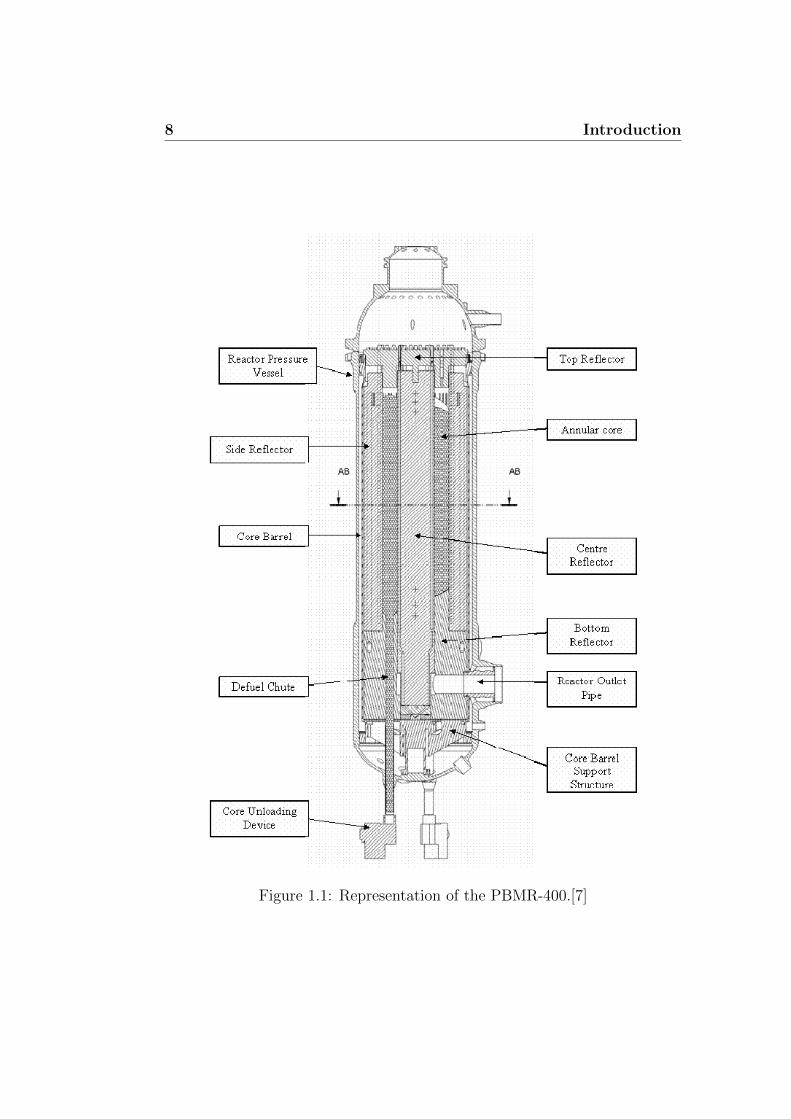
The High Temperature Reactor (HTR-10) began operation in the year2003. It was designed as a prototype for a commercial scale 250 MW mod-ular reactor. Current research is focussed on two pebble-bed reactors. Onetype is situated in China, the High Temperature Reactor-Pebblebed Mod-ules (HTR-PM), designed to produce 250 MW of thermal energy per module.Construction started in 2009 and completion is expected in 2013. The othertype is located in South-Africa, the Pebble-bed Modular Reactor (PBMR-400), of which a schematic view is given in figure 1.1. The design started in1999, but due to financial problems, the design process has slowed down. ThePBMR-400 is only in its design phase, but a lot of computational work hasbeen done on this reactor type, because it has been made a computationalbenchmark [7]. Steady-state and transient situations regarding the thermo-hydrolics and neutronics have been computed and serve as a benchmark forCFD programs focussed on pebble-beds.

1.2 Previous Research

Computational research on pebble-bed reactors is necessary because physicalexperiments with pebble-bed reactors cannot provide a full description ofthe pebble-bed, without altering the set-up. Without a full description of apebble-bed reactor, it cannot be used safely.

Determining the flow around all of the pebbles inside the reactor core,in the order of 100.000 to several million pebbles, is a task far out of thecurrent computational reach. Some CFD calculations focus on small parts of

1.3. Aim of this Thesis 7

the reactor, determining the flow around several pebbles and using this in-formation to extrapolate behavior in the total pebble-bed [15]. This methodgives precise information of local heat gradients, but fails to give a goodmacroscopic view of the reactor. Other methods depend on using a two-phase porous medium approach, describing the porous medium only by theporosity [12]. This makes it possible to get a good macroscopic view of thebehavior inside the reactor, such as wall channeling and non-uniform powerdensity, but microscopic effects cannot be calculated [13].

However, computations on pebble-bed reactors have yielded different re-sults than the actual testreactors for low temperature pebble-bed reactors[16]. A better understanding of the CFD of pebble-bed reactors is thereforeneeded.

1.3 Aim of this Thesis

This thesis focusses on an open-source CFD program called OpenFOAM. Aspecial solver has been developed within OpenFOAM, to solve equations gov-erning the mass and heat transfer inside pebble-beds, describing the pebble-bed as a two-phase steady-state porous medium.

The objective of this research is to determine if the solver is capable ofsolving heat and mass transfer inside a pebble-bed reactor correctly. This isdone with several testcases, three analytical cases and one physical experi-ment, based on the experiment of Achenbach. Finally the total code is testedon the PBMR computational benchmark, to examine if the code calculateswhat the benchmark suggests.

1.4 Thesis Outline

This thesis will first cover the equations determining the behavior of thepebble-bed. Then the implementation of these equations in the solver isdiscussed, along with information of CFD in general and specifically aboutOpenFOAM. Three analytical test cases are examined, regarding the one-dimensional pressure drop, Poiseuille flow and one-dimensional heat transfer.An experiment, done by Achenbach [1], is computed and the PBMR is sim-ulated [7]. Afterwards a conclusion and recommendation for future researchwill be given.

8 Introduction

Figure 1.1: Representation of the PBMR-400.[7]

Chapter 2

Governing Equations

The pebble-bed solver is based on a model consisting of a set of equations,which are detailed in this chapter. The equations are based on conservationof momentum, energy and mass.

2.1 Conservation of Momentum and Mass

The velocity field is governed by conservation of momentum, in its compressi-ble form [6].

φ(∇u)︸︷︷︸c.a.

+Fporu︸︷︷︸p.d.

+ εT︸︷︷︸s.s.t.

= −ε∇p︸︷︷︸p.g.

(2.1)

The first part of this equation is the convective acceleration term, using themass flux φ = ερ|u|, where ε is the porosity, ρ the density and u the velocity(c.a.). The porous drag is a function of Fpor, which covers the resistance dueto porous media (p.d.). The shear stress term is a function of the deviatoricstress tensor, T (s.s.t.). Finally the pressure gradient depends on the fluidpressure, p (p.g.).

The porous drag term depends on the porous drag force, Fpor. The re-lation of the Fpor is a combination of two parts, the first part is the viscousflow (Carman and Kozeny) and the last part is the turbulent flow (Burke andPlummer), and was combined by Ergun in 1952, see equation 2.2 [2] [11].

Fpor =150µ(1− ε)2

ε2d2peb

+1.75(1− ε)ρ|u|

ε2dpeb(2.2)

Investigation by Achenbach and the German nuclear service, KTA, resulted

10 Governing Equations

in another relation, see equation 2.3 [1].

Fpor =160µ(1− ε)3

εd2peb

+3µ0.1(1− ε)2.1ρ0.9|u0.9|

εd1.1peb

(2.3)

Both equations for the porous drag force show, respectively, a viscous and aturbulent flow part. The code used in this thesis uses Ergun’s equation, eq.2.2.

Conservation of mass is used to correct the pressure and velocity fields,eq. 2.4, which will be explained in section 3.4.3.

∇ · φ = ∇ · (ερu) = 0 (2.4)

2.2 Conservation of Energy

The temperature of the coolant is considered by conservation of energy, byapplying this on the enthalpy field of the coolant and using h = cpT , wherecp is the specific heat.

φ · (∇h)︸︷︷︸c.e.

−∇ · (εαeff∇h)︸︷︷︸d.e.

= htc(Tpeb − THe)︸︷︷︸h.t.

+φ

ρ· ∇p︸︷︷︸

p.g.

(2.5)

The first term considers the convection of enthalpy, using mass flux φ andenthalpy h (c.e.), followed by the diffusion of enthalpy, using the porosity ε,the thermal diffusivity α and the enthalpy, h (d.e.). The heat transfer termuses the heat transfer coefficient, htc, and the difference between the pebbletemperature Tpeb and coolant temperature THe (h.t.). The pressure gradientuses mass flux, φ, density ρ and pressure gradient, p (p.g.) [6].

Empirical formulas are used to calculate the fluid properties in the code,see equations 2.6 to 2.10

htc =αcpNu(1− ε)

6d2peb

(2.6)

αeff =0.11ρdpeb(ε− 1)|u|

(0.39− 1)(2.7)

Nu = (1 + 1.5(1− ε)) (2.8)2 +

√√√√(0.664√RePr1/3)2 +

(0.037Re0.9Pr)2

Re0.1 + 2.443(Pr2/3 − 1)

Re =

dpebρ|u|µ

(2.9)

Pr =µcpk

(2.10)

2.3. Pebble Temperature Equation 11

The heat transfer coefficient, htc, determines the heat exchange betweenthe pebbles and the fluid and is modeled according to the relation given byGnielinski [17]. αeff gives the effective diffusion of enthalpy and uses therelation from Yagi and Kunii [18]. The Nusselt number Nu refers to theratio between convective and conductive heat transfer, which is necessaryfor the heat transfer coefficient, where dpeb is the pebble diameter, µ is thekinematic viscosity, and k is the thermal conductivity and is calculated withthe equation from Gnielinski [17]. Pr and Re are the Prandtl and Reynoldsnumbers, respectively.

2.3 Pebble Temperature Equation

To calculate the temperature of the pebbles the following equation is used.

−∇ · (kpeb∇Tpeb)︸︷︷︸d.t.

+htc(Tpeb − THe)︸︷︷︸h.t.

= Q︸︷︷︸source

(2.11)

The left side contains the diffusion of heat between the pebbles and usesthe pebble-bed conductivity kpeb, which includes the heat transfer due toradiation between the pebbles, and the internal heat transfer of the pebbles(d.t). The pebble-pebble heat transfer through contact points is not includedas it is considered negligible compared to the high radiative heat transferat high pebble temperatures in the pebble-bed. The next term calculatesthe heat transfer from the pebbles to the coolant (h.t.). The right side ofthe equation contains the source term, Q, which is the power generated byfission inside the pebbles in W/m3. The porosity may approach 1 in near-wallsituations, which makes the thermal conductivity approach infinity. For thesesituations special near-wall formulas are used. The thermal conductivity ofgraphite inside the pebble-bed is given by Zehner and Schluender [20], andthe thermal conductivity of graphite near the walls is given by Tsotsas andMartin [21].

kwithingraphite = 4σT 3dpeb (2.12)(1−√

(1− ε))

+

√(1− ε)2εr− 1

(Bz + 1

Bz

)1 +1(

2εr− 1

)Λ

−1

knear−wallgraphite =4σT 3dpeb(

2εr− 1

) (1−√

(1− ε))

+√

(1− ε)

14σT 3dpeb

( 2εr−1)

+1

pg

−1

(2.13)

12 Governing Equations

Where σ is the Stefan-Boltzmann constant, εr is the emissivity of the pebbles,which is 0.8 and Bz, Λ, and pg are given in equations 2.14, 2.15, and 2.16.

Bz = 1.25(

1− εε

)10/9

(2.14)

Λ =pg

4σT 3dpeb(2.15)

pg = 108.901− 0.188285T + 2.79606 · 10−4T (2.16)

−2.18888 · 10−7T 3 + 6.6 · 10−11T 4

Chapter 3

Solving the Equations withOpenFOAM

The equations governing the physics of pebble-beds discussed in chapter 2 donot have an analytical solution - except in extremely simplified cases - andneed to be solved computationally. In our case this has been done with the aidof the open source software package OpenFOAM. The implementation of theequations in OpenFOAM and the methods used to solve them numericallyare discribed below.

First an introduction is given on the various methods generally used tosolve computational fluid dynamics (CFD) problems. The next section de-scribes the OpenFOAM software package, followed by an explanation of theschemes used to discretize the various equations of chapter 2. The last sec-tion details the implementation of the equations in the my pebbleBedFoamsolver and how this system of equations is solved.

3.1 Introduction to CFD

The equations defining the behavior of the pebble-bed, and generally thebehavior of fluid mechanics inside the given geometry, often consist of differ-ential equations, which demand special ways of approaching. For approxi-mating these problems and geometries, a certain discretization method needsto be chosen. Over the years, several discretization methods have been in-vented, all having their strong and weak points, of which the most importantare:

• Finite Difference Method

• Finite Volume Method

14 Solving the Equations with OpenFOAM

• Finite Element Method

These discretization methods rely on a mesh to be able to solve. A mesh is acollection of points, at a given distance from each other, covering the entireobject of interest. This mesh does not need to be uniformly distributed ororthogonal, but non-uniformity and non-orthogonality need to be taken intoconsideration at the discretization schemes. For greater accuracy and detailthe grid can be made finer at places of interest, see [4].

3.1.1 Finite Difference Method

This is the oldest method of solving partial differential equations, discoveredby Euler in the 18th century, and is based on approximations of the partialderivatives between nodal points within the mesh. This method starts offwith the conservation laws in a differential form. The mesh with this methodis mainly based in structured grids, which are also used as coordinate lines.The downside of this method is that the conservation laws are not enforced,unless special care is taken.

3.1.2 Finite Volume Method

This method devides the mesh into small volumes, with in its center a node.The conservation laws are stated in an integral form using single volume cellsand use Gauss’ Theorem to switch from volume to surface integrals. Thismethod requires interpolation to determine the values at the edges of thecontrol volume. The advantage of this method is that the surface integralsat both sides of the boundary need to be the same, which makes it easyto enforce the conservation laws. The disadvantage is the fact that thiscode relies on three calculation methods, namely integration, interpolationand differentiation, making the code more difficult. OpenFOAM, the CFDprogram used in this thesis, is based on the FV method.

3.1.3 Finite Element Method

This method is similar to the Finite Volume Method, because the domain isspatially discretisized and considered with the use of volume integrals, butdepends on a piecewise function between all nodal points that satisfies thedifferential equation. This gives a function defined everywhere in the domain,and not only on the nodes. The advantage of this method is the fact thatit can be used on any grid, regardless of geometry. A drawback is that forsimpler grids it is more difficult to find efficient solution methods.

3.2. A Quick Tour in OpenFOAM 15

3.2 A Quick Tour in OpenFOAM

OpenFOAM is a C++ based CFD code, which relies on the Finite VolumeMethod. One of the greatest advantages of OpenFOAM is that it is open-sourced. This means everybody can change the code to the way he/sheprefers. Much configuration has to be done by the user, but this gives a lotof freedom compared to commercial packages [5].

The Basic Format

OpenFOAM is run on a UNIX cluster. Two directories are of importance,namely the case directory and the solver directory. The case directory con-tains the situation dependant information, such as the boundary and initialconditions, the mesh and discretization methods. The solver directory con-tains the files in which the equations governing the case and their solutionsteps are defined. The files in the solver are converted into an executablewhich can be run in the case directory. The output can either be viewedwith a text editor or with a visualization program.

3.3 Discretization Schemes

In CFD the problems need to be discretized, because computational methodsrely on solving discrete quantities instead of continuous functions. Space,time, and the equations need to be adapted to discrete parts. Time dis-cretization will not be considered in this thesis, because only steady-statesituations are evaluated. Space discretization will be done with the use of amesh. This splits the domain into a set of cells that fill and bound it. Beforethe equations can be solved on the mesh, they need to be discretized. Theoperators are also discretized. This section will explain the operators usedin the code in OpenFOAM [4] [13] [23].

3.3.1 Interpolation

Interpolation is necessary for FV solvers because values are stored at thecenters of the volumes, but are sometimes needed on the faces of the volume.Two different interpolation schemes are implemented in OpenFOAM:

• Central Differencing: a weighted mean between two nodes

• Upwind Differencing: uses the value of the node upstream.


Upwind differencing is a faster method and has inherent stability, yet has asmaller accuracy than central differencing. Central differencing is best usedon course meshes, but can give instability in non-orthogonal meshes.

3.3.2 Gradient

Just as interpolation, the gradient, ∇φ, can be calculated with two differ-ent methods. The first method considers Gauss’ theorem and examines thegradient with the use of volume and surface integration.∫

V∇φdV =

∫SφdS ≈

∑f

Sfφf (3.1)

The V and S boundaries of integration are the volume and surface domainsof the cell, f is the index of the cell faces. The sum over f is the sum overall the cell faces, with φf the variable of interest on the cell face, times thesurface face vector, Sf .

The second method divides the difference between two nodes, by thedistance between the two nodes.

φN − φP|d|

= ∇⊥f φ (3.2)

The difference between the cell of interest, P, and the neighboring cell, N,divided by the cell size, |d|, gives the divergence perpendicular to the face,thus in the direction of the surface face vector. In case the mesh is non-orthogonal a correction term needs to be considered.

3.3.3 Divergence

The divergence is considered over a volume-cell with Gauss’ theorem.∫V∇ · φdV ≈

∑f

Sf · φf (3.3)

3.3.4 Laplacian

The laplacian is considered over a volume cell, which, with Gauss’ theorem,is converted into an inner product between the gradient and surface vector.∫

V∇ · ∇φ ≈

∑f

Sf · ∇φf (3.4)

3.4. The Solver: my pebbleBedFoam 17

3.3.5 Source Term

The source term, indicating production or destruction of a variable, can bea general function of φ. Going from the general linearization to the, for FVschemes necessary, integral form.

Sφ = φSI + SE →∫VSφ(φ)dV = SIVPφP + SEVP (3.5)

Sφ is the linearised source term, governed by SI and SE, respectively theimplicit and explicit source terms, and VP is the volume of the cell. Theimplicit term, SI , uses the the current iteration’s variables. The explicit term,SE, uses previous iteration’s variables. Both variables may be a function ofthe previous iteration’s φ.

3.3.6 Under-Relaxation

Under-relaxation is a trick used to prevent large fluctuations between itera-tions. It is based on adding less than the total correction of an iteration to avariable, by a factor of α, the relaxation factor. This may cause convergenceto occur slower, but guarantees stability for sufficiently low α.

φnew = φold + αφcorrection (3.6)

Note that 0 < α ≤ 1

3.4 The Solver: my pebbleBedFoam

my pebbleBedFoam is the name of the pebble-bed solver that was tested inthis thesis. The solver runs the subsolvers in this specific order:

• calculate UEqn.H, governing the momentum transfer.

• calculate hEqn.H, governing the heat transfer of the coolant.

• calculate pEqn.H, governing the pressure-momentum coupling.

• calculate TpebEqn.H, governing the pebble temperature.

These sequence will be iterated, until the solution is converged. The followingsubsections will explain the equations that are solved by the code.


3.4.1 UEqn.H

Regarding the velocity field, conservation of momentum, eq. 2.1, is rewrittento facilitate solving the equation for u.

∇ · (φu)− (∇ · φ) u + Fporu + εT = −ε∇p (3.7)

This equation is solved with the explicit p value. This u field does notobey the continuity equation, eq. 2.4, which will be corrected for in thepEqn routine. The equation is solved with a relaxation factor of 0.8 and the∇ · (φu) term uses the Gauss scheme with upwind differencing, or simplyGauss upwind.

3.4.2 hEqn.H

First of all this sub-solver updates the values of α and cp and recalculates thevalues of Pr, Re, Nu, htc and αeff , with equations 2.6 to 2.10. The coolantenergy conservation equation, eq. 2.5, has been rewritten to make it moresuitable for computational calculation.

∇ · (φh)− (∇ · φ)h−∇ · (εαeff∇h) +htc

cph = ∇ ·

(φ

ρp

)(3.8)

−P∇ ·(φ

ρ

)+ htcTpeb

After solving this equation for h, the temperature effects on physical parame-ters are updated, and the sub-solver is done. This equation uses a relaxationfactor of 0.9. The ∇ · (φh) term is approximated with Gauss upwind, the∇ · (εαeff∇h) term is approximated with Gauss linear, using central differ-encing and ρ is interpolated with the use of central differencing.

3.4. The Solver: my pebbleBedFoam 19

3.4.3 pEqn.H

The pEqn calculates the pressure field and adjusts the velocity field so itobeys the continuity equation, eq. 2.4. This subroutine uses the SIMPLE-algorithm to compute the pressure and velocity fields [4] [10].

The SIMPLE Algorithm

The momentum equation, eq. 2.1, is written down in a matrix notation, eq.3.9.

AuiP un+1i,P +

∑l

Auil un+1i,l = Qn

ui−(δpn

δxi

)P

(3.9)

In this equation A is the matrix representation of equation 2.1, u indicatesthe velocity field, Q indicates a source term, p is the pressure field, and x isthe cell width of the gradient. The P index indicates the node in questionand the l index indicates the neighboring nodes. The i index denotes thedirection of u and x.

In the code, current values for the pressure and source terms are notknown, so the values of previous computations are used. Rewriting equation3.9, with the use of m = n+1, and using the fact that the source and pressureterms use previously computed values, results in equations 3.10 and 3.11.

um∗i,P =Qm−1ui−∑lA

uil u

m∗i,l

AuiP− 1

AuiP

(δpm−1

δxi

)P

(3.10)

um∗i,P = um∗i,P −1

AuiP

(δpm−1

δxi

)P

(3.11)

The use of the asterisk, ∗, indicates that this value is not yet the final valueof u, because it does not obey continuity yet. The first term on the righthand side of equation 3.10 is replaced by u for convenience.

The continuity equation, eq. 2.4, can be rewritten to equation 3.12

δρumiδxi

= 0 (3.12)

In this equation umi is the new velocity field, which obeys continuity. This canbe rewritten as equation 3.13, where pm is the new pressure field. Insertingthis in equation 3.12 results in equation 3.14.

umi,P = um∗i,P −1

AuiP

(δpm

δxi

)P

(3.13)

δ

δxi

[ρ

AuiP

(δpm

δxi

)]P

=

[δρum∗iδxi

]P

(3.14)


This equation can be solved for the pressure field p, and with this correctedpressure, a correction for the velocity can be computed, using the updatedversion of equation 3.11, equation 3.13. The new velocity field obeys con-tinuity, but not necessarily conservation of momentum 2.1. With the newpressure field, a new um∗i can be calculated, and again a new pressure field.This process is iterated until the pressure and velocity fields are converged.

This solver uses a lot of unstable mathematics, so a low relaxation coeffi-cient of 0.22 is used. The mass flux φ is interpolated with central differencingand the pressure laplacian, ∇2

(ε2ρpAui

)is evaluated with the Gauss central dif-

ferencing scheme.

3.4.4 TpebEqn.H

This subroutine calculates λg and kpeb, eq. 2.13, followed by equation 3.15.

htc(Tpeb − THe) = ∇2(kpebTpeb) +Q (3.15)

A relaxation factor of 0.9 is used on the pebble temperature and the laplacianuses the Gauss gradient method, with linear interpolation.

Chapter 4

Test Cases

The code is verified with the use of several test cases. Each test case focuseson certain parts of the code. The momentum equation is tested with theuse of a one-dimensional pressure drop case and a two dimensional case,concerning laminar flow between parallel plates. To conclude the momentumpart of the code, an experiment done by Achenbach is simulated. The thermalpart of the code is tested by a one-dimensional heat transfer case.

4.1 One-Dimensional Pressure Drop

This calculation concerns the pressure drop in a one dimensional case, whichhas the benefit it has a simple analytical solution. Besides verification ofthe pressure drop, the dependence on mesh size and measuring position areexamined.

4.1.1 Set up, Measurement & Expectations

The geometry consists of a one-dimensional column of 1.4 m high. From 0.2m to 1.2 m the porosity is 0.39 and the first and last 0.2 m the porosity is1, so the flow field can stabilize. The pebble diameter is 0.06 m. The fluidproperties are kept constant, with µ = 10−5 kgm−1s−1 and ρ = 1 kgm−3.The velocity is varied between 0.02 and 10 ms−1, resulting in a Reynoldsnumber distribution from 120 to 60000. To investigate the effect of cell size,the mesh size is varied between 140, 280, 700 and 1400 cells. Additionally, forthe 1400 mesh the pressure drop is calculated over three different intervalsfor the 1400 cell mesh:

• total field: The pressure difference between the in- and outlet of thedomain.

22 Test Cases

• porosity field: The pressure difference between the begin and end partof the porous field.

• derivative: The pressure gradient in the middle of the porous field.

The pressure drop should follow the analytical solution, given by Ergun’sequation, eq. 2.2. The dependence on the mesh size is unknown, as is thedependence on the measuring position.

4.1.2 Results

The results of the measuring position computations are displayed as a relativedifference between the analytical solution and the calculated value, see figure4.1. This figure shows that the derivative in the pebble-bed is in excellentagreement with Ergun’s equation. The pressure drop over the whole domainand the pressure drop over the porous field show some error, with the biggestrelative error in the pressure drop between the begin and end of the pebble-bed. For almost all Reynold numbers the pressure drop over the porousregion is larger than over the total field.

This behavior is caused by unstable regions caused by the discrete transi-tion of porosity at the beginning and end of the porous region. This discretetransition causes fluctuations in the pressure and velocity fields, which causegreater errors on the transition position than over the total bed.

The results of the mesh dependance are displayed in figure 4.2. This com-putation uses the relative difference of the total field with Ergun’s analyticalsolution, eq 2.2. The reciprocal relative difference is plotted against the meshsize. The result is a linear relationship, which indicates a 1

nodesrelationship.

A possible explanation is that the unstable regions, causing the inaccuracies,always have the same length in nodes. When the number of nodes increases,the percentage of nodes that have unstable behavior decreases as 1

r.

4.1. One-Dimensional Pressure Drop 23

Figure 4.1: The relative difference be-tween the analytical solution and thecomputed value plotted against theReynolds number

Figure 4.2: The reciprocal relative dif-ference between the analytical solu-tion and the computed value plottedagainst the mesh size for a Reynoldsnumber of 120

24 Test Cases

4.2 Two-Dimensional Laminar Flow Between

Parallel Plates

This computation concerns the perpendicular velocity of a laminar flow be-tween two parallel plates. For this experiment, the expected solution isPoiseuille flow, see equation 4.1.

4.2.1 Set Up, Measurements & Expectations

The geometry consists of two parallel plates, through which a fluidum flows.The plates are 0.01 m apart and are 1 m long. A no slip boundary conditionexists on the plates and the inlet velocity is 1 ms−1, which is distributeduniformly. The fluid properties are kept constant, with µ = 10−3 kgm−1s−1,ρ = 1 kgm−3 and since there is no pebble bed, the porosity is 1. This resultsin a Reynolds number of 10. The mesh is 200 cells in the flow direction and50 cells perpendicular to the flow direction.

Poiseuille flow, see equation 4.1, is expected for the perpendicular velocity,since the mesh size should be adequate and the Reynolds number is wellwithin the laminar flow range. The analytical solution for this case is:

ux =1

2µ

dp

dx

y2 −(d

2

)2 (4.1)

ux is the flow in the flow direction, µ is the dynamic viscosity, dpdx

is pressuregradient in the flow direction and the last term describes the distance fromthe walls, where y is the radial distance, and d is the distance between the twoplates. The Poiseuille flow has a quadratic distribution. The computationwill be compared to the quadratic solution, to check whether it fits poiseuilleflow.

4.2.2 Results

The flow field between the two plates is displayed in figure 4.3. The fluidflow first has to stabilize, because the velocity field is uniform at the inlet.

Figure 4.3: The fluid velocity in the flow direction, red indicates high veloc-ities, blue indicates low velocities

4.2. Two-Dimensional Laminar Flow Between Parallel Plates 25

Figure 4.4: The data points of the velocity distribution(data), fitted by aquadratic function(quadratic).

The velocity profile is examined at 0.8 m from the inlet, see figure 4.4. Itis also fitted by a quadratic distribution, eq. 4.1. The sum of the absoluteerrors is 0.06 %, which means this test case is in excellent agreement withthe expected analytical solution.

26 Test Cases

4.3 Achenbach’s Experiment

Achenbach measured the pressure drop over a packed bed in a physical ex-periment for Reynolds ranging from 150 to 3 ∗ 105 and compared his resultswith the pressure drop relation from the KTA, see equation 2.3 [1]. This testcase will compare the code to the experimental data gathered by Achenbach.


The geometry consists of a 1.4 m high cylinder, with a radius of 0.5 m. Thefirst and last 0.2 m have porosity 1, the pebble-bed has a uniform porosityof 0.39 and a pebble diameter of 0.06 m. The fluid is air, at a constanttemperature of 293 K. The velocity on the walls has the slip boundarycondition and the inlet velocity ranges from 0.1 to 25.6 ms−1. Two outletpressures are used of 105 and 106 Pa. Different outlet pressures are used,because if the pressure drop is in the order of the outlet pressure, the pressuredrop affects the fluid properties. The mesh consists of 70 nodes in the flowdirection, 50 nodes in the radial direction, and uses a wedge symmetry planeto simulate a cylinder.

In the experiment done by Achenbach, [1], a measure for the pressuredrop is given by the use of the pressure drop coefficient, ψ, see equation 4.2

ψ =2dpebρ|u|2

(ε3

1− ε

)∆p

∆h(4.2)

The paper concludes with a relationship for ψ, see equation 4.3, which is theKTA relation for the pressure drop [1].

ψ =320Re1−ε

+6(

Re1−ε

)0.1 (4.3)

The data Achenbach gathered in his experiment and his fit through the dataare displayed in figure 4.5. This data will be used for code comparison. Thepaper of Achenbach notes that the relation, eq. 4.3, does not describe hismeasurements for Reynolds numbers higher than 8 ∗ 104. The computedresults are expected to follow Ergun’s equation, eq. 2.2, since this equationis used in the code.

4.3. Achenbach’s Experiment 27

Figure 4.5: The data Achenbach gathered in his experiment and his fit of thedata. The o indicate measurements at atmospheric pressure, the x indicatemeasurements at higher pressure.

4.3.2 Results

The results of the computation are plotted in figure 4.6 and in table 4.1. Forthe low pressure situation, the computational result and the analytical resultstart to diverge for Reynolds numbers of 2 ∗ 104. For the high pressure situ-ation, the computational and analytical result start to diverge for Reynoldsnumbers of 2 ∗ 105. The divergence for higher Reynolds numbers is becausethe pressure drop over the domain is high compared to the outlet pressure,resulting in significant change in the density over the domain, see table 4.1.

Figure 4.6: The pressure drop coefficient according to the analytical Ergunequation (ψ ergun), the computed data (ψ ergun computed), the KTA rela-tion, and the data gathered by Achenbach.

28 Test Cases

Table 4.1: The Reynolds number, ψ, pressure drop, inlet density and outletpressure(low (105)) or high (106)) of the computation of Achenbach’s exper-iment

Re ψ ∆p ρ pout[−] [−] [Pa] [kgm−3] [Pa]196 4.49 1 1.1863 105

392 3.96 4 1.1863 105

785 3.71 15 1.1865 105

1570 3.58 58 1.1869 105

3147 3.52 229 1.1890 105

6335 3.50 918 1.1970 105

13035 3.52 3800 1.2314 105

29648 3.67 18049 1.4004 105

67655 4.13 72402 2.0452 105

3920 3.54 36 11.863 106

19620 3.48 883 11.865 106

39270 3.48 3538 11.870 106

78800 3.51 14340 12.032 106

159640 3.68 60944 12.580 106

340590 4.68 330164 15.780 106

Ergun’s equation and the KTA relation, and thus the measurements, startto diverge for a Reynolds number of around 400. The PBMR case expectsReynolds numbers of around 4 ∗ 104. When the measured data and Ergun’srelation are compared at this Reynolds number, ψ differs by a factor of100.31

100.54= 1.70. An error of a factor 1.70 can be expected at the PBMR test

case [7].

4.4. Analytical Heat Transfer 29

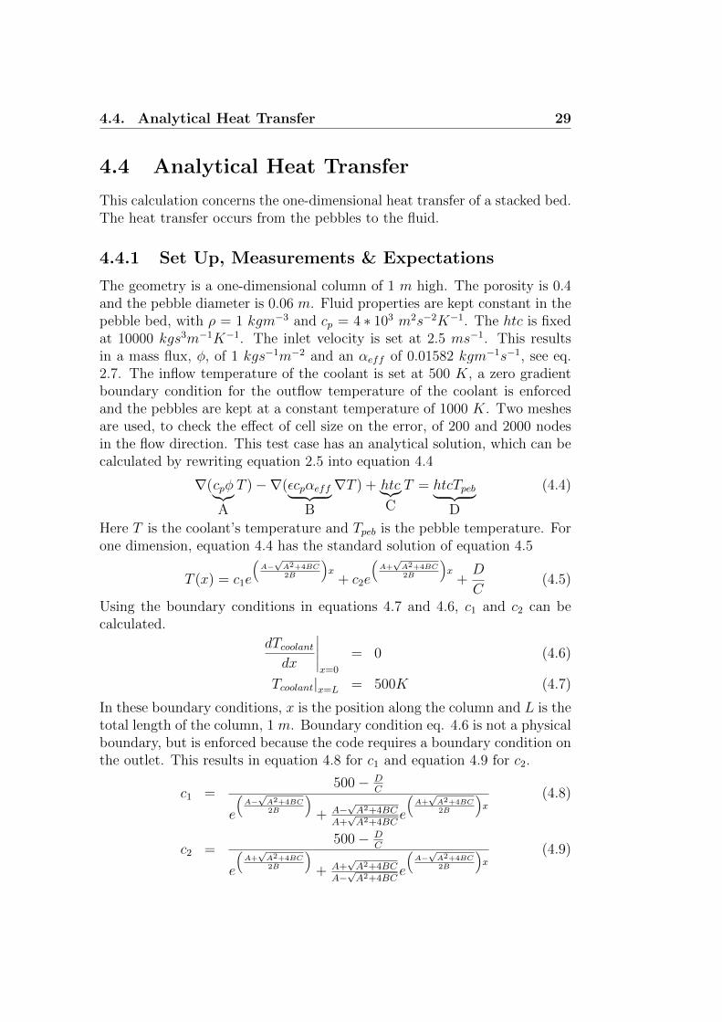
4.4 Analytical Heat Transfer

This calculation concerns the one-dimensional heat transfer of a stacked bed.The heat transfer occurs from the pebbles to the fluid.


The geometry is a one-dimensional column of 1 m high. The porosity is 0.4and the pebble diameter is 0.06 m. Fluid properties are kept constant in thepebble bed, with ρ = 1 kgm−3 and cp = 4 ∗ 103 m2s−2K−1. The htc is fixedat 10000 kgs3m−1K−1. The inlet velocity is set at 2.5 ms−1. This resultsin a mass flux, φ, of 1 kgs−1m−2 and an αeff of 0.01582 kgm−1s−1, see eq.2.7. The inflow temperature of the coolant is set at 500 K, a zero gradientboundary condition for the outflow temperature of the coolant is enforcedand the pebbles are kept at a constant temperature of 1000 K. Two meshesare used, to check the effect of cell size on the error, of 200 and 2000 nodesin the flow direction. This test case has an analytical solution, which can becalculated by rewriting equation 2.5 into equation 4.4

∇(cpφ︸︷︷︸A

T )−∇(εcpαeff︸︷︷︸B

∇T ) + htc︸︷︷︸C

T = htcTpeb︸︷︷︸D

(4.4)

Here T is the coolant’s temperature and Tpeb is the pebble temperature. Forone dimension, equation 4.4 has the standard solution of equation 4.5

T (x) = c1e

(A−√A2+4BC2B

)x

+ c2e

(A+√A2+4BC2B

)x

+D

C(4.5)

Using the boundary conditions in equations 4.7 and 4.6, c1 and c2 can becalculated.

dTcoolantdx

∣∣∣∣∣x=0

= 0 (4.6)

Tcoolant|x=L = 500K (4.7)

In these boundary conditions, x is the position along the column and L is thetotal length of the column, 1 m. Boundary condition eq. 4.6 is not a physicalboundary, but is enforced because the code requires a boundary condition onthe outlet. This results in equation 4.8 for c1 and equation 4.9 for c2.

c1 =500− D

C

e

(A−√A2+4BC2B

)+ A−

√A2+4BC

A+√A2+4BC

e

(A+√A2+4BC2B

)x

(4.8)

c2 =500− D

C

e

(A+√A2+4BC2B

)+ A+

√A2+4BC

A−√A2+4BC

e

(A−√A2+4BC2B

)x

(4.9)

30 Test Cases

Figure 4.7: The temperature profile ofthe computation and of the analyticalsolution

Figure 4.8: The relative error betweenthe computational result and the ana-lytical solution

4.4.2 Results

The results are plotted in figures 4.7 and 4.8. Figure 4.7 shows the compu-tational temperature profile and is compared to the analytical solution, eq.4.5. Figure 4.8 shows the difference between the computational result andthe analytical solution.

The computational result and the analytical solution are in good com-parison, with a maximum difference of 0.04%. The relative difference showsan increase in error near the outlet. This is because the code forces zerogradient between the node and the wall. The analytical solution has zerogradient on the wall, so there is a difference in position. For the large mesh,the error is less than for a the small mesh, as expected.

This test case shows that the code is capable of calculating the heattransfer through helium correctly.

Chapter 5

Pebble-Bed Modular Reactor

The Pebble-Bed Modular Reactor (PBMR) is an international benchmark,based on the PBMR-400MW design. It is a code-to-code comparison totest different CFD codes. The tests on the PBMR concern steady-state andtransient processes, but this case will only focus on the steady-state processes[7].

5.1 Set Up, Measurement & Expectations

The geometry is an axisymmetric cylinder, with a height of 11.5 m, an innerradius of 1 m and an outer radius of 1.85 m. The first 0.5 m from the inlethas a porosity of 1. The packed bed, from 0.5 to 11.5 m has a porosity of 0.39and a pebble radius of 0.06 m. The helium inlet mass flux is 192.7 kgs−1 andthe outlet pressure is 9 MPa. Using the fluid properties of helium at 9 MPa,a velocity of 4.291 ms−1 is found. The inlet temperature of the coolant is773 K and the power distribution is given in figure 5.1, with a total powerof 400 MW [7].

The benchmark suggests simulating a 2 m thick graphite wall, with anouter temperature of 293 K, as a boundary condition for the outer wall. Thiscannot be simulated by the code, so two methods will be used to account forthis.

• Zero Gradient: No wall heat flux, by forcing a zero gradient on bothwalls.

• Fixed Value: Fixed outer wall temperature, supplied by previous CFDresults from the benchmark. The inner wall temperature has a zerogradient boundary condition.

32 Pebble-Bed Modular Reactor

Figure 5.1: The power density profile inside the PBMR reactor. The left sideis towards the reactor center [3].

A 230 by 50 cells mesh is used. Most computations of the benchmark suggestan outlet helium temperature of 1172 K, an average helium temperature of1022 K, an average pebble temperature of 1042 K and a pressure drop of2.75 bar.

5.2 Results

The results of the CFD code will be discussed in three sections, first dis-cussing the helium temperature, followed by the pebble temperature andfinally the pressure drop.

5.2.1 Helium Temperature

The numerical results of the benchmark case are given in table 5.1. Thistable contains the average helium temperature of the total porous regionand from the outlet, the average pebble temperature, and the pressure dropof the benchmark and of the two computations. The helium temperatureprofiles in the axial and in the radial direction can be seen in figures 5.2 and5.3.

Table 5.1: The results of the PBMR computation, with the fixed value caseand zero gradient case compared with the benchmark results.

Fixed Value Case Zero Gradient Case BenchmarkT Helium Outlet [K] 1159.3 1153.7 1172T Helium Average [K] 1011.9 1007.6 1022T Pebble Average [K] 1034.2 1030.0 1042Pressure Drop [Pa] 4.80∗105 4.77∗105 2.75∗105

5.2. Results 33

Figure 5.2: The average helium tem-perature in the axial direction of thefixed value and zero gradient case,compared with the average, minimumand maximum benchmark tempera-tures.

Figure 5.3: The average helium tem-perature in the radial direction of thefixed value and zero gradient case,compared with the average, minimumand maximum benchmark tempera-tures.

Table 5.1 shows that the outlet and average fixed value temperatures arehigher than the zero gradient temperatures. This means the pebble-bed isheated by the fixed value boundary condition on the outer wall. Althoughboth cases and the benchmark provide similar temperature profiles, the fixedvalue and the zero gradient cases result in different outlet temperatures thanthe benchmark suggests, with a maximum temperature difference of around20 K at the outlet. This is outside of the minimum value of the benchmark’scomputations.

The temperature difference is caused by the absorption of energy due toexpansion. The benchmark’s computations do not account for this. Thetemperature difference of 20 K can also be shown by equation 5.1. In thisequation the difference in thermal outlet energy is compared to the energythe fluid absorbs when it expands through the pebble-bed. A specific heatof 5195 m2s−2K−1 is used, and the density at the in- and outlet are 4.525kgm−3 and 4.295 kgm−3 respectively. A constant temperature of 1000 Kand a pressure drop of 5 bar are assumed.

mcp∆T = Q =∫ V2

V1pdV ≈ p∆V = (φ∆t)

(1

ρ1

− 1

ρ2

)p (5.1)

∆T =

(1

ρ2

− 1

ρ1

)p

cp=(

1

4.295− 1

4.525

)9 ∗ 106

5195= 20.5K


Table 5.2: The results of the computation with the pressure gradient termturned off in the enthalpy equation, for two cases and compared with thebenchmark.

Fixed Value Case Zero Gradient Case BenchmarkT Helium Outlet [K] 1176.0 1174.8 1172T Helium Average [K] 1019.3 1016.5 1022T Pebble Average [K] 1041.5 1038.8 1042Pressure Drop [Pa] 4.80∗105 4.77∗105 2.75∗105

To verify that the pressure gradient term in equation 2.5 is indeed thecause for the low average and output temperature of the helium, this termwas turned off and the computations were repeated. This resulted in theexpected behavior, see table 5.2. The temperature differences between thecases and the benchmark are similar to the differences between the differentcomputations of the benchmark.

The radial profiles of both cases do not match the benchmark, and thecode’s results are outside the outer values of the benchmark’s computations.The fixed value boundary condition on the outer wall matches the expectedresult, because it’s value is enforced. The temperature difference at theouter wall for the zero gradient case is around 20 K, which is caused bythe absorption of energy due to expansion, see equation 5.1. The differenceat the inner wall is higher, which is because the benchmark uses a differentboundary condition on the inner wall.

5.2. Results 35

5.2.2 Pebble Temperature

The pebble temperature profiles can be seen in figures 5.4 and 5.5. Thepebble temperature profiles show wrinkles, which arise from the discrete stepsin the power density field. The temperature profiles of both cases follow thebenchmark’s lowest temperature profile, in both the axial and the radialdirection.

The average pebble temperatures can be found in table 5.1, and showthat both cases result in a lower average temperature than the benchmarksuggests. When the pressure gradient is turned off in the code, see table 5.2the temperature of both cases and the benchmark differ less. Besides thepressure gradient term, a different formula for the Nusselt number, eq. 2.9,is used in the benchmark, and the code uses a slightly simplified relation forthe pebble-pebble heat transfer, eq. 2.11, but this does not seem to have asignificant effect.

Figure 5.4: The average pebble tem-perature in the axial direction of thefixed value and zero gradient case,compared with the average, minimumand maximum benchmark tempera-tures.

Figure 5.5: The average pebble tem-perature in the radial direction of thefixed value and zero gradient case,compared with the average, minimumand maximum benchmark tempera-tures.


5.2.3 Pressure Drop

The pressure drop profile can be seen in figure 5.6 and the effective pressuredrops can be seen in table 5.1. The pressure profiles and the pressure dropof the fixed value and zero gradient case differ from the benchmark.

Both pressure drops are around 4.8∗105 Pa, compared to a pressure dropof 2.75 ∗ 105 Pa for the benchmark. Figure 4.6 of the Achenbach testcaseshowed a ratio between the Ergun and KTA relation, at a Reynolds numberof 4∗104, of

ψErgunψKTA

= 1.70. The ratio between pressure drops is∆pComputation∆pBenchmark

=1.75, which shows the different pressure drop relations are indeed the causeof the different pressure drops.

Figure 5.6: The pressure profile of the PBMR case for the fixed value and zerogradient case, compared with the average, minimum and maximum pressureprofiles of the benchmark.

Chapter 6

Conclusions

A code implemented in OpenFOAM was investigated using several simpletest cases with analytical or experimental solutions, and by calculating thePBMR steady state thermohydraulics benchmark.

6.1 Experimental Conclusions

Comparison of the code for the simple test cases showed the code evaluatesthe equations implemented in the solver with good accuracy, with one excep-tion. The one-dimensional test case for the pressure drop pointed out thatnear discrete transitions in porosity, such as at the top of a pebble bed, fluc-tuations arise in the pressure and velocity fields. As these fluctuations arelocal and pebble-bed reactors are large, the influence of these fluctuations issmall.

The results of the PBMR case differed on several points with those re-ported by the participants. Firstly, the coolant and pebble temperature fieldswere on average 20 K lower. This difference was caused by the inclusion ofthe expansion term in the helium heat transfer equation, causing additionalcooling of the coolant. This expansion term was not included in the bench-mark, although our calculations show this term should not be ignored.

Also, the results for the pressure drop over the pebble bed showed a 75% higher pressure drop over the pebble-bed. This difference is because thecode uses Ergun’s relation and the benchmark uses the KTA relation. As seenin the Achenbach case, the KTA relation closely follows the measurement.Ergun’s relation, however predicts a significantly higher pressure drop athigher Reynolds numbers, with a difference of 70 % for Reynolds numbers of4 ∗ 104, comparable to the Reynolds numbers in the PBMR.

Finally, as the code was not yet capable of calculating heat transfer

38 Conclusions

through the central and side reflector, artificial boundary conditions wereused at the walls of the pebble bed. This, together with different relationsfor the Nusselt number for the heat transfer from the pebbles to the coolantand a slightly simplified relation for the pebble-pebble heat transfer, resultedin small differences in the radial pebble and helium temperature profiles.

Still, the axial coolant and pebble temperature profiles were in good agree-ment with the results from the benchmark participants which, together withthe good results from the analytical test cases, brings us to the conclusionthat the solver implemented in OpenFOAM can be used to compute heatand mass transfer in a pebble-bed reactor, especially if Erguns equation forthe pressure drop is replaced by KTA’s relation.

6.2 Future Research

This research leaves some questions unanswered, which could be interestingfor further investigation.

• Discrete steps in porosity result in fluctuations of the pressure andvelocity fields. A different approach to these discrete steps may resultin less fluctuation.

• The porosity in the PBMR benchmark is uniform. In actual pebble-bed reactors porosity approaches one near the walls, causing a differentflow pattern. Computations with non-uniform porosity can determinewhat effect this has.

• The PBMR benchmark states different relations than the relations usedin the code. Changing the relations in the code to the relations sug-gested by the benchmark could verify if the code can provide the sameresults as the benchmark.

• The term for pebble-pebble interactions through contact in the equa-tion for the diffusion of heat between the pebbles has been neglected,because it was thought to have negligible influence. A study to theheat transfer through touching pebbles could determine if this approx-imation was justified.

• The code was unable to simulate heat transfer through a graphite re-flector, and therefore unable to calculate the heat flux through the wallin the manner suggested by the benchmark. Adapting the code to beable to simulate this reflector could check whether the code is capableof calculating the radial temperature profile correctly.

Bibliography

[1] E. Achenbach, Heat and flow characteristics of packed beds, Institute ofEnergy Process Engineering, Julich, Germany, (1994)

[2] S. Ergun, Fluid flow through placed columns, Chemical engineeringprogress, 48(2):90-98, (1952)

[3] PBMR-400 Data Exercise Sheet 2, OECD/NEA/NSC, (2006)

[4] J.H. Ferziger and M. Peric. Springer, Computational Methods for FluidDynamics, 3rd Edition, (2002)

[5] OpenFOAM User Guide, OpenCFD, Version 1.7.1, (2010)

[6] Bird, Steward, Lightfoot, Transport Phenomena, Chemical EngineeringDepartment University of Winsconsin-Madison, John Wiley and SonsInc. 2nd Edition, (2002)

[7] PBMR coupled neutronics/thermal hydraulics transient benchmark thePBMR-400 core design - Benchmark edition, OECD/NEA/NSC, (2007)

[8] Donald A. Nield, Adrian Bejan, Convection in Porous Media, Springer,(2006)

[9] L.P.B.M. Janssen, M.M.C.G. Warmoeskerken, Transport PhenomenaData Companion, VSSD, (2006)

[10] T. Craft, Pressure-Velocity Coupling, Lecture Notes

[11] Flow through porous passages, Fluid Mechanics, Tutorial #4,www.freestudy.co.uk

[12] CG du Toit, The Flow and Heat Transfer in a Packed Bed High Tem-perature Gas-Cooled Reactor., North-West University, (2010)

40 Bibliography

[13] C.J. Visser, Modelling Heat and Mass Flow Through Packed Pebble Beds:A Heterogeneous Volume Averaged Approach, University of Pretoria,(2007)

[14] S. Ergun and A.A. Orning, Fluid Flow through Randomly PackedColumns and Fluidized Beds, Carnegie Institute of Technology, (1949)

[15] T. Frederikse, CFD Calculations on the helium cooling of the Pebble BedReactor Core, TU Delft, (2010)

[16] A safety re-evaluation of the AVR pebble bed reactor operation and itsconsequences for future HTR concepts, Berichte des ForschungszentrumsJulich, (2008)

[17] V. Gnielinski, Equations for the calculation of heat and mass transferduring flow, through stationary spherical packings at moderate and highPclet number, International Chemical Engineering, Vol. 21, pp. 378-383,(1981)

[18] S. Yagi and D. Kunii, Studies on effective thermal conductivities inpacked beds, American Institute for Chemical Engineers, Volume 3, Issue3, pages 373-381, (1957)

[19] S. Yagi and N. Wakao, Heat and mass transfer from walls to fluid inpacked beds, American Institute for Chemical Engineers, Volume 5, Issue1, pages 79-85, (1959)

[20] Heat transport and afterheat removal for gas cooled reactors under acci-dent conditions, IAEA-TECDOC-1163, section 4.2.2

[21] E. Tsotsas and H. Martin, Thermal conductivity of packed beds: A Re-view, Institute fur Thermische Verfahrenstechnik, Universitat Karlsruhe,(1987)

[22] G.Dietrich, W. Neumann, N. Rohl, Decommissioning of the Tho-rium High Temperature Reactor (THTR-300), Hochtempeartur-Kernkraftwerk GmbH

[23] H. Rusche, Computational Fluid Dynamics of Dispersed Two-PhaseFlows at High Phase Fractions, Department of Mechanical Engineering,Imperial College London, (2002)

testing a nuclear pebble-bed reactor model in … this research investigates whether the cfd code...

Documents