test series: march, 2019 mock test paper 1 final course ... · 6 optimal schedule is- marriage...
TRANSCRIPT

1
Test Series: March, 2019
MOCK TEST PAPER – 1
FINAL COURSE: GROUP – II
PAPER – 5: ADVANCED MANAGEMENT ACCOUNTING
SUGGESTED ANSWERS/HINTS
1. (a) Let Cx be the Contribution per unit of Product X.
Therefore Contribution per unit of Product Y =Cy=4/5Cx = 0.8Cx
Given F1 + F2 = 1,50,000,
F1 = 1,800Cx (Break even volume × contribution per unit)
Therefore F2 = 1,50,000 – 1,800Cx.
3,000Cx –F1 =3,000 × 0.8Cx – F2 or 3,000Cx – F1 =2,400 Cx-F2 (Indifference point)
i.e., 3,000Cx – 1,800Cx = 2,400Cx – 1,50,000 + 1,800Cx
i.e., 3,000Cx = 1,50,000, Therefore Cx = Rs.50/- (1,50,000 / 3,000)
Therefore Contribution per unit of X = Rs.50
Fixed Cost of X = F1 = Rs.90,000 (1,800 × 50)
Therefore Contribution per unit of Y is Rs.50 × 0.8 = Rs.40 and
Fixed cost of Y = F2 = Rs.60,000 (1,50,000 – 90,000)
The value of F1 = Rs.90,000, F2 = Rs.60,000 and X = Rs.50 and Rs.40
(b) Following acceptance by early innovators, conventional consumers start following
Situation Appropriate Pricing Policy
(i) ‘A’ is a new product for the company and the market and meant for large scale production and long term survival in the market. Demand is expected to be elastic.
Penetration Pricing
(ii) ‘B’ is a new product for the company, but not for the market. B’s success is crucial for the company’s survival in the long term.
Market Price or Price Just Below Market Price
(iii) ‘C’ is a new product to the company and the market. It has an inelastic market. There needs to be an assured profit to cover high initial costs and the unusual sources of capital have uncertainties blocking them.
Skimming Pricing
(iv) ‘D’ is a perishable item, with more than 80% of its shelf life over.
Any Cash Realizable Value*
(*) this amount decreases every passing day.
(c) Product A & B are joint products and produced in the ratio of 1:2 from the same direct material-
C.
Production of 40,000 additional units of B results in production of 20,000 units of A.
Calculation of Contribution under existing situation
Particulars Amount (Rs.) Amount (Rs.)
Sales Value:
A – 2,00,000 units @ Rs.25 per unit
B – 4,00,000 units @ Rs.20 per unit
50,00,000
80,00,000
1,30,00,000
© The Institute of Chartered Accountants of India

2
Less: Material- C (12,00,000 units@ Rs.5 per unit)
Less: Other Variable Costs
Contribution
60,00,000
42,00,000
28,00,000
Let Minimum Average Selling Price per unit of A is Rs.X
Calculation of Contribution after acceptance of additional order of ‘B’
Particulars Amount (Rs.) Amount (Rs.)
Sales Value:
A – 2,20,000 units @ Rs. X per unit
B – 4,00,000 units @ Rs.20 per unit
40,000 units @ Rs.15 per unit
Less: Material- C (12,00,000 units x 110%) @ Rs.5 per unit
Less: Other Variable Costs (Rs.42,00,000 x 110%)
Contribution
2,20,000 X
80,00,000
6,00,000
2,20,000 X + 86,00,000
66,00,000
46,20,000
2,20,000 X – 26,20,000
Minimum Average Selling Price per unit of A
Contribution after additional order of B = Contribution under existing production
2,20,000 X – 26,20,000 = 28,00,000
2,20,000 X = 54,20,000
X = 54,20,000
2,20,000 = Rs.24.64
Minimum Average Selling Price per unit of A is Rs.24.64
(d) Primal
Minimize
Z = 2x1 − 3x2 + 4x3
Subject to the Constraints
3x1 + 2x2 + 4x3 ≥ 9
2x1 + 3x2 + 2x3 ≥ 5
−7x1 + 2x2 + 4x3 ≥ − 10
6x1 − 3x2 + 4x3 ≥ 4
2x1 + 5x2 − 3x3 ≥ 3
−2x1 − 5x2 + 3x3 ≥ − 3
x1, x2, x3 ≥ 0
Dual:
Maximize
Z = 9y1 + 5y2 − 10y3 + 4y4 + 3y5 − 3y6
Subject to the Constraints:
3y1 + 2y2 − 7y3 + 6y4 + 2y5 − 2y6 ≤ 2
© The Institute of Chartered Accountants of India

3
2y1 + 3y2 + 2y3 − 3y4 + 5y5 − 5y6 ≤ − 3
4y1 + 2y2 + 4y3 + 4y4 − 3y5 + 3y6 ≤ 4
y1, y2, y3, y4, y5, y6 ≥ 0
By substituting y5−y6= y7 the dual can alternatively be expressed as:
Maximize
Z =
9y1 + 5y2 − 10y3 + 4y4 + 3y7
Subject to the Constraints:
3y1 + 2y2 − 7y3 + 6y4 + 2y7 ≤ 2
−2y1 − 3y2 − 2y3 + 3y4 − 5y7 ≥ 3
4y1 + 2y2 + 4y3 + 4y4 − 3y7 ≤ 4
y1, y2, y3, y4 ≥ 0, y7 unrestricted in sign.
2. (a) (i) Calculation of ‘Total Labour Hours’ over the Life Time of the Product
‘Kitchen Care’
The average time per unit for 250 units is
Yx = axb
Y250 = 30 × 250 -0.3219
Y250 = 30 × 0.1691
Y250 = 5.073 hours
Total time for 250 units = 5.073 hours × 250 units
= 1,268.25 hours
The average time per unit for 249 units is
Y249 = 30 × 249–0.3219
Y249 = 30 × 0.1693
Y249 = 5.079 hours
Total time for 249 units = 5.079 hours × 249 units
= 1,264.67 hours
Time for 250th unit = 1,268.25 hours – 1,264.67 hours
= 3.58 hours
Total Time for 1,000 units = (750 units × 3.58 hours) + 1,268.25 hours
= 3,953.25 hours
(ii) Profitability of the Product ‘Kitchen Care’
Particulars Amount (Rs.) Amount (Rs.)
Sales (1,000 units) 50,00,000
Less: Direct Material 18,50,000
Direct Labour (3,953.25 hours × Rs.80) 3,16,260
Variable Overheads (1,000 units× Rs.1,000) 10,00,000 31,66,260
© The Institute of Chartered Accountants of India

4
Contribution 18,33,740
Less: Packing Machine Cost 5,00,000
Profit 13,33,740
(iii) Average ‘Target Labour Cost’ per unit
Particulars Amount (Rs.)
Expected Sales Value 50,00,000
Less: Desired Profit (1,000 units × Rs.800) 8,00,000
Target Cost 42,00,000
Less: Direct Material (1,000 units × Rs.1,850) 18,50,000
Variable Cost (1,000 units × Rs.1,000) 10,00,000
Packing Machine Cost 5,00,000
Target Labour Cost 8,50,000
Average Target Labour Cost per unit
(Rs.8,50,000 ÷ 1,000 units)
850
(b) Activities P and Q are called duplicate activities (or parallel activities) since they have the same
head and tail events. The situation may be rectified by introducing a dummy either between P
and S or between Q and S or before P or before Q (i.e. introduce the dummy before the tail event
and after the duplicate activity or Introduce the dummy activity between the head event and the
duplicate activity). Possible situations are given below:
© The Institute of Chartered Accountants of India

5
3. (a) The objective of the given problem is to identify the preferences of marriage parties about halls
so that hotel management could maximize its profit.
To solve this problem first convert it to a minimizat ion problem by subtracting all the elements of
the given matrix from its highest element. The matrix so obtained which is known as loss matrix is
given below-
Loss Matrix/Hall
Marriage Party 1 2 3 4
A 0 2,500 X X
B 5,000 0 5,000 12,500
C 7,500 0 10,000 5,000
D 0 5,000 X X
Now we can apply the assignment algorithm to find optimal solution. Subtracting the minimum
element of each column from all elements of that column-
Loss Matrix/Hall
Marriage Party 1 2 3 4
A 0 2,500 X X
B 5,000 0 0 7,500
C 7,500 0 5,000 0
D 0 5,000 X X
The minimum number of lines to cover all zeros is 3 which is less than the order of the square
matrix (i.e.4), the above matrix will not give the optimal solution.
Subtracting the minimum uncovered element (2,500) from all uncovered elements and add it to
the elements lying on the intersection of two lines, we get the following matrix -
Loss Matrix/Hall
Marriage Party 1 2 3 4
A 0 0 X X
B 7,500 0 0 7,500
C 10,000 0 5,000 0
D 0 2,500 X X
Since the minimum number of lines to cover all zeros is 4 which is equal to the order of the
matrix, the below matrix will give the optimal solution which is given below-
Loss Matrix/Hall
Marriage Party 1 2 3 4
A 0 0 X X
B 7,500 0 0 7,500
C 10,000 0 5,000 0
D 0 2,500 X X
© The Institute of Chartered Accountants of India
6
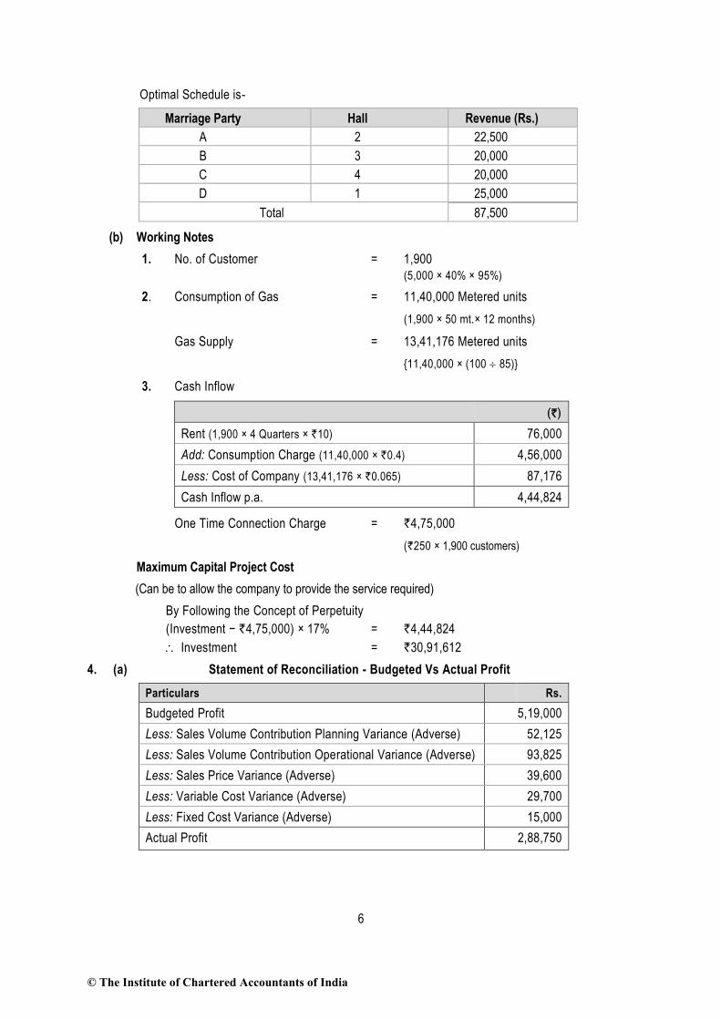
Optimal Schedule is-
Marriage Party Hall Revenue (Rs.)
A 2 22,500
B 3 20,000
C 4 20,000
D 1 25,000
Total 87,500
(b) Working Notes
1. No. of Customer = 1,900
(5,000 × 40% × 95%)
2. Consumption of Gas = 11,40,000 Metered units
(1,900 × 50 mt.× 12 months)
Gas Supply = 13,41,176 Metered units
{11,40,000 × (100 85)}
3. Cash Inflow
(`)
Rent (1,900 × 4 Quarters × `10) 76,000
Add: Consumption Charge (11,40,000 × `0.4) 4,56,000
Less: Cost of Company (13,41,176 × `0.065) 87,176
Cash Inflow p.a. 4,44,824
One Time Connection Charge = `4,75,000
(`250 × 1,900 customers)
Maximum Capital Project Cost
(Can be to allow the company to provide the service required)
By Following the Concept of Perpetuity
(Investment − `4,75,000) × 17% = `4,44,824
Investment = `30,91,612
4. (a) Statement of Reconciliation - Budgeted Vs Actual Profit
Particulars Rs.
Budgeted Profit 5,19,000
Less: Sales Volume Contribution Planning Variance (Adverse) 52,125
Less: Sales Volume Contribution Operational Variance (Adverse) 93,825
Less: Sales Price Variance (Adverse) 39,600
Less: Variable Cost Variance (Adverse) 29,700
Less: Fixed Cost Variance (Adverse) 15,000
Actual Profit 2,88,750
© The Institute of Chartered Accountants of India

7
Workings
Basic Workings
Budgeted Market Share (in %) = 2,00,000units
4,00,000units = 50%
Actual Market Share (in %) = 1,65,000units
3,75,000units= 44%
Budgeted Contribution = Rs.21,00,000 – Rs.12,66,000
= Rs.8,34,000
Average Budgeted Contribution (per unit) = Rs.8,34,000
Rs.2,00,000= Rs.4.17
Budgeted Sales Price per unit = Rs.21,00,000
Rs.2,00,000= Rs.10.50
Actual Sales Price per unit = Rs.16,92,900
Rs.1,65,000= Rs.10.26
Standard Variable Cost per unit = Rs.12,66,000
Rs.2,00,000= Rs.6.33
Actual Variable Cost per unit = Rs.10,74,150
Rs.1,65,000= Rs.6.51
Calculation of Variances
Sales Variances:
Volume Contribution Planning* = Budgeted Market Share % × (Actual Industry
Sales Quantity in units – Budgeted Industry Sales
Quantity in units) × (Average Budgeted
Contribution per unit)
= 50% × (3,75,000 units – 4,00,000 units) × Rs.4.17
= Rs. 52,125 (A)
(*) Market Size Variance
Volume Contribution Operational** = (Actual Market Share % – Budgeted Market
Share %) × (Actual Industry Sales Quantity in
units) × (Average Budgeted Contribution per unit)
= (44% – 50%) × 3,75,000 units × 4.17
= Rs. 93,825 (A)
(**) Market Share Variance
Price = Actual Sales – Standard Sales
= Actual Sales Quantity × (Actual Price – Budgeted
Price)
= 1,65,000 units × (Rs.10.26 – Rs.10.50)
= Rs.39,600 (A)
© The Institute of Chartered Accountants of India

8
Variable Cost Variances:……….
Cost = Standard Cost for Production – Actual Cost
= Actual Production × (Standard Cost per unit –
Actual Cost per unit)
= 1,65,000 units × (Rs.6.33 – Rs.6.51)
= Rs.29,700(A)
Fixed Cost Variances:
Expenditure = Budgeted Fixed Cost – Actual Fixed Cost
= Rs.3,15,000 – Rs.3,30,000
= Rs.15,000 (A)
Fixed Overhead Volume Variance does not arise in a Marginal Costing system
(b) The Δ ij matrix or Cij – (ui + vj) matrix, where Cij is the cost matrix and (u i + vj) is the cell
evaluation matrix for unallocated cell.
The Δ ij matrix has one or more ‘Zero’ elements, indicating that, if that cell is brought into the
solution, the optional cost will not change though the allocation changes.
Thus, a ‘Zero’ element in the Δ ij matrix reveals the possibility of an alternative solution.
5. (a) 1. Projected Raw Material Issues (Kg):
‘N’ ‘O’ ‘P’
‘L’ (48,000 units-Refer Note) 60,000 24,000 ---
‘M’ (36,000 units-Refer Note) 72,000 - 54,000
Projected Raw Material Issues 1,32,000 24,000 54,000
Note:
− Based on this experience and the projected sales, the DTSML has budgeted production of
48,000 units of ‘L’ and 36,000 units of ‘M’ in the sixth period.
= 52,500 x 40% + 45,000 – 18,000 = 48,000
= 27,000 x 40% + 42,000 – 16,800 = 36,000
− Production is assumed to be uniform for both products within each four-week period.
2. and 3. Projected Inventory Activity and Ending Balance (Kg):
‘N’ ‘O’ ‘P’
Average Daily Usage 6,600 1,200 2,700
Beginning Inventory 96,000 54,000 84,000
Add: Orders Received:
Ordered in 5th period 90,000 - 60,000
Ordered in 6th period 90,000 - -
Sub Total 276,000 54,000 144,000
Less: Issues 132,000 24,000 54,000
Projected ending inventory balance 144,000 30,000 90,000
© The Institute of Chartered Accountants of India

9
Note:
− Ordered 90,000 Kg of ‘N’ on fourth working day.
− Order for 90,000 Kg of ‘N’ ordered during fifth period received on tenth working day.
− Order for 90,000 Kg of ‘N' ordered on fourth working day of sixth period received on
fourteenth working day.
− Ordered 30,000 Kg of ‘O’ on eighth working day.
− Order for 60,000 Kg of ‘P’ ordered during fifth period received on fourth working day.
− No orders for ‘P’ would be placed during the sixth period.
4. Projected Payments for Raw Material Purchases:
Raw Material
Day/Period Ordered
Day/Period Received
Quantity Ordered
Amount Due (Rs.)
Day/Period Due
‘N’ 20th/5th 10th /6th 90,000 Kg 90,000 20th/6th
‘P’ 4th/5th 4th /6th 60,000 Kg 60,000 14th/6th
‘N’ 4th/6th 14th /6th 90,000 Kg 90,000 4th/7th
‘O’ 8th/6th 13th /7th 30,000 Kg 60,000 3rd/8th
(b) Statement of Profitability
Product Sales Value
(Rs.)
P / V Ratio
(%)
Contribution
(Rs.)
A 2,50,000 50 1,25,000
B 4,00,000 40 1,60,000
C 6,00,000 30 1,80,000
Total 12,50,000 4,65,000
Less: Fixed Overheads 5,02,200
Profit / (Loss) (37,200)
Additional Sale Value of each Product
Product Sales Value (Rs.)
A Rs. 74,400 (Rs.37,200 ÷ 0.5)
B Rs. 93,000 (Rs.37,200 ÷ 0.4)
C Rs.1,24,000 (Rs.37,200 ÷ 0.3)
Additional Total Sales Value maintaining the same Sale – Mix
= Rs.37,200 ÷ 0.372*
= Rs.1,00,000
* Combined P / V Ratio = Total Contribution
100Total Sales
= Rs. 4,65,000
100Rs.12,50,000
= 37.2%
© The Institute of Chartered Accountants of India

10
6. (a) Cumulative Average Time for 256 parts = 48.43 hrs.*
[112.50 × (0.908)]
Total Time for 256 parts = 12,398.08 hrs.
[48.43 hrs.× 256 parts]
Total Labour Cost of 256 parts = Rs.2,47,961.60
[12,398.08 hrs.× Rs.20]
Revised Labour Cost for zero profit = Rs.3,22,961.60
[Rs.2,47,961.60 + Rs.75,000]
Total Time for 256 parts (Revised) = 16,148.08 hrs.
[Rs.3,22,961.60/ Rs.20]
Cumulative Average Time for 256 parts (Rev.) = 63.08 hrs.
[16,148.08/256]
The usual learning curve model is
y = axb
Where y = Cumulative Average Time per part for x parts
a = Time required for first part
x = Cumulative number of parts
b = Learning coefficient (log r/log 2)
Accordingly 63.08 = 112.50× (256) b
0.5607 = 28b
log 0.5607 = log 28b
log 0.5607 = 8 × b × log2
log 0.5607 = 8 ×logr
log2
× log 2
log 0.5607 = 8 log r
log 0.5607 = log r8
0.5607 = r8
r = 8 0.5607
r = 0.9302
Learning Rate (r) = 93.02%.
Therefore
Sensitivity = 3.02/90
= 3.36%
Students may also take 48.38 hrs. (112.50 0.43)
© The Institute of Chartered Accountants of India

11
(b) Calculation showing Rates for each Activity
Activity Activity
Cost [a]
(Rs.)
Activity Driver No. of Units
of Activity
Driver [b]
Activity Rate
[a] / [b]
(Rs.)
Providing ATM Service 1,00,000 No. of ATM Transactions 2,00,000 0.50
Computer Processing 10,00,000 No. of Computer Transactions 25,00,000 0.40
Issuing Statements 8,00,000 No. of Statements 5,00,000 1.60
Customer Inquiries 3,60,000 Telephone Minutes 6,00,000 0.60
Calculation showing Cost of each Product
Activity Checking Accounts (Rs.)
Personal Loans
(Rs.)
Gold Visa
(Rs.)
Providing ATM Service 90,000
(1,80,000 tr. x 0.50)
--- 10,000
(20,000 tr. x 0.50)
Computer Processing 8,00,000
(20,00,000 tr. x 0.40)
80,000
(2,00,000 tr. x 0.40)
1,20,000
(3,00,000 tr. x 0.40)
Issuing Statements 4,80,000
(3,00,000 st. x 1.60)
80,000
(50,000 st. x 1.60)
2,40,000
(1,50,000 st. x 1.60)
Customer Inquiries 2,10,000
(3,50,000 min. x 0.60)
54,000
(90,000 min. x 0.60)
96,000
(1,60,000 min. x 0.60)
Total Cost [a] Rs.15,80,000 Rs.2,14,000 Rs.4,66,000
Units of Product [b] 30,000 5,000 10,000
Cost of each Product [a] / [b] 52.67 42.80 46.60
7. (a) Target cost is the difference between the estimated selling price of a proposed product with
specified functionality and quality and target margin. This is a cost management technique that
aims to produce and sell products that will ensure the target margin. It is an integral part of the
product design. While designing the product the company allocates value and cost to different
attributes and quality. Therefore, they use the technique of value engineering and value analysis.
The target cost is achieved by assigning cost reduction targets to different operations that are
involved in the production process. Eventually, all operations do not achieve the cost reduction
targets, but the overall cost reduction target is achieved through team work. Therefore, it is said
that target costing fosters team work.
(b) (i) The company has done extensive exercise in year-I that can be used as a basis for
budgeting in year-II by incorporating increase in costs / revenue at expected activity level.
Hence, Traditional Budgeting would be more appropriate for the company in year-II.
(ii) In Traditional Budgeting system budgets are prepared on the basis of previous year’s
budget figures with expected change in activity level and corresponding adjustment in the
cost and prices. But under Zero Base Budgeting (ZBB) the estimations or projections are
converted into figures. Since, sales manager is unable to substantiate his expectations into
figures so Traditional Budgeting would be preferred against Zero Base Budgeting.
(iii) Zero Base Budgeting would be appropriate as ZBB allows top-level strategic goals to be
implemented into the budgeting process by tying them to specific functional areas of the
organization, where costs can be first grouped, then measured against previous results and
current expectations.
© The Institute of Chartered Accountants of India

12
(iv) Zero Base Budgeting allocates resources based on order of priority up to the spendi ng cut-
off level (maximum level upto which spending can be made). In an organisation where
resources are constrained and budget is allocated on requirement basis, Zero Base
Budgeting is more appropriate method of budgeting.
(c) If unit variable cost and unit selling price are not constant then the main problem that would arise
while fixing the transfer price of a product would be as follows:
There is an optimum level of output for a firm as a whole. This is so because there is a certain
level of output beyond which its net revenue will not rise. The ideal transfer price under these
circumstances will be that which will motivate these managers to produce at this level of output.
Essentially, it means that some division in a business house might have to produce its output at a
level less than its full capacity and in all such cases a transfer price may be imposed centrally.
(d) Direct Product Profitability (DPP) is ‘Used primarily within the retail sector, and involves the attribution of both the purchase price and other indirect costs such as distribution, warehousing, retailing to each product line. Thus a net profit, as opposed to a gross profit, can be identified for each product. The cost attribution process utilises a variety of measures such as warehousing space, transport time to reflect the resource consumption of individual products.’
Benefits of Direct Product Profitability:
(i) Better Cost Analysis - Cost per product is analysed to know the profitability of a particular
product.
(ii) Better Pricing Decision- It helps in price determination as desired margin can be added with
the actual cost.
(iii) Better Management of Store and Warehouse Space- Space Cost and Benefit from a product
can be analysed and it helps in management of store and warehouse in profitable way.
(iv) The Rationalisation of Product Ranges etc.
(e) Random Number Assignment
Daily Demand Days Probability Cumulative Probability Random No. Assigned
4 4 0.08 0.08 00 − 07
5 10 0.20 0.28 08 − 27
6 16 0.32 0.60 28 − 59
7 14 0.28 0.88 60 − 87
8 6 0.12 1.00 88 − 99
Simulation Table
Day Random No. Demand No. of Cars on Rent Rent Lost
1 15 5 5 ---
2 48 6 6 ---
3 71 7 6 1
4 56 6 6 ---
5 90 8 6 2
Total 29 3
Average no. of Cars Rented are 5.8 29Cars
5
Rental Lost equals to 3 Cars
© The Institute of Chartered Accountants of India