test of global market efficiency, through momentum, oscillation, and...
TRANSCRIPT
TEST OF GLOBAL MARKET EFFICIENCY, THROUGH MOMENTUM, OSCILLATION, AND
RELATIVE STRENGTH INDEX STRATEGIES
Frank Shui Ting Chu Bachelor of Business Administration
Simon Fraser University, 2003
PROJECT SUBMITTED IN PARTIAL FULFILLMENT OF THE REQUIREMENTS FOR THE DEGREE OF
MASTER OF ARTS
In the Department
of Economics
O Frank Shui Ting Chu 2004
SIMON FRASER UNIVERSITY
Fall 2004
All rights reserved. This work may not be reproduced in whole or in part, by photocopy
or other means, without permission of the author.
APPROVAL
Name: Frank Shui Ting Chu
Degree: M. A. (Economics)
Title of Project : Test Of Global Market Efficiency, Through Momentum, Oscillation, And Relative Strength Index Strategies
Examining Committee:
Chair: Ken Kasa
Geoffery Poitras Senior Supervisor
John Heaney Supervisor
- -
Robbie Jones Internal Examiner
Date Approved: Tues, November 30,2004
. . 11

SIMON FRASER UNIVERSITY
PARTIAL COPYRIGHT LICENCE
The author, whose copyright is declared on the title page of this work, has granted to Simon Fraser University the right to lend this thesis, project or extended essay to users of the Simon Fraser University Library, and to make partial or single copies only for such users or in response to a request from the library of any other university, or other educational institution, on its own behalf or for one of its users.
The author has further granted permission to Simon Fraser University to keep or make a digital copy for use in its circulating collection.
The author has further agreed that permission for multiple copying of this work for scholarly purposes may be granted by either the author or the Dean of Graduate Studies.
It is understood that copying or publication of this work for financial gain shall not be allowed without the author's written permission.
Permission for public performance, or limited permission for private scholarly use, of any multimedia materials forming part of this work, may have been granted by the author. This information may be found on the separately catalogued multimedia material and in the signed Partial Copyright Licence.
The original Partial Copyright Licence attesting to these terms, and signed by this author, may be found in the original bound copy of this work, retained in the Simon Fraser University Archive.
W. A. C. Bennett Library Simon Fraser University
Bumaby, BC, Canada

ABSTRACT
This paper tests the weak-form global market efficiency, by comparing the
returns of technical trading strategies to the returns of buy-and-hold strategies on 24
country indexes and 1 world index. The technical trading strategies examined in this
paper include static and dynamic momentum approaches, oscillation strategy, and
Relative Strength Index strategy. Empirical testing suggests that it is possible for the
trading strategies to sigruficantly outperform the buy-and-hold strategy in
some country indexes and even the world index. However, no excessive profits are
extracted in United States and Germany from all the technical trading strategies, noting
that these countries are weak-form efficient in the context of this paper. Furthermore,
the techrucal trading strategies do not work well during extreme expansionary periods,
but they are useful in filtering losses during recessionary periods.

ACKNOWLEDGEMENTS
First of all, I want to thank Professors Geoffrey Poitras and Robert Grauer of the
Faculty of Business Administration for the tremendous support and valuable advice
they have given me in this paper. They were a great influence in bringing me to
business and finance; I admire them both immensely. I am also very grateful for the
help of Professor Robert Jones of the Department of Economics and Professor John
Heaney of the Faculty of Business Administration.
Lastly, I want to thank my family for all the love and encouragement they have
given me; my friends who have always supported me; and all my students in SFU who
have given me a sense of fulfillment.

TABLE OF CONTENTS
. . ............................................................................................................................ Approval 11
... Abstract ............................................................................................................................. 111
Acknowledgements .......................................................................................................... iv
.............................................................................................................. Table of Contents v
List of Abbreviations ....................................................................................................... vi
1 Introduction ............................................................................................................... 1
...................................................... 2 Overview of Momentum and Mean-Reversion 3
2.1 Explanations of Momentum ................................................................................ 4 ........................................................................ 2.2 Explanations of Mean-Reversion 8
3 Methodology and Empirical Approach ................................................................ 11
............................................................................... 3.1 Static Momentum Strategy 13 ................................................................ 3.2 Semi-Dynamic Momentum Strategy 15
.......................................................................... 3.3 Dynamic Momentum Strategy 16 . .
3.4 Oscillation Strategy ........................................................................................... 17 ...................................................................... 3.5 Relative Strength Index Strategy 18
4 Data .......................................................................................................................... 20
5 Results and Summary ........................................................................................... 21
..................................... 5.1 Full Period Returns of the Technical Trade Strategies 21 5.2 Return of All the Strategies Listed Yearly ........................................................ 23 5.3 Test Result for the Static Momentum Strategy ................................................. 24 5.4 Test Result for the Semi-Dynamic Momentum Strategy .................................. 25
........................................... 5.5 Test Result for the Dynamic Momentum Strategy 25 5.6 Test Result for the Oscillation Strategy ............................................................ 26
........................................ 5.7 Test Result for the Relative Strength Index Strategy 26
6 Discussion and Conclusion .................................................................................... 27
. ............................................................................................... Appendix Result Tables 30
Reference List .................................................................................................................. 40

LIST OF ABBREVIATIONS
N = - n -
D =
DD =
EMA =
RSI =
RS =
MR =
MM =
Y =
s - -
t - -
total number of observations the nth observation / each specific time excessive profit daily difference of stock price exponential moving average relative strength index relative strength mean-reversion momentum the mean under null hypothesis standard deviation t-stat
Subscripts c = each specific country i = each specific technical trading strategy h = the buy and hold strategy n = the nth observation / time subscribe

INTRODUCTION
In 1970, Fama's work called "Efficient Capital Markets: a Review of Theory and
Empirical Work" created a financial field of study of market efficiency. He distinguishes
financial markets into three forms of market efficiency - the strong form, the semi-
strong-form, and the weak-form market efficiency. The efficient market is defined as the
market where the stock prices would always "fully reflect" all available information.
The weak-form market efficiency, which this paper focuses on, is more specifically
defined as a situation where past prices and returns cannot predict the future price and
return. In other words, the technical analysis is worthless as it is impossible to
consistently extract excessive profits using the chart, the trend, the historic prices, and
the statistical analysis.
Many studies were published regarding testing the weak-form market efficiency.
In order to show weak-form market inefficiency, the studies have tried to uncover
evidences of abnormal profits from technical analyses. Thaler (1987) approaches it
through the January effect and Thaler (1987), French (1980) also examine the anomalies
associated with weekend, holiday, turn of the month, and intraday effects. Some
analysts employ the performance ratios like price-earning ratio, and price-to-book ratio.
Some use momentum and mean-reversion strategies, which will be discussed in later
sections of this paper. Chordia and Shivakumar (2002) employ the test with return
predictability from macrovariables. Some of these studies show market inefficiency, but
some of the evidence are mixed.

This paper in general will employ two types of technical analysis strategies: the
momentum strategy and the mean-reversion strategy. The momentum anomaly will
branch out into the static, semi-dynamic, and dynamic momentum strategies and also
the oscillation strategy. The mean-reversion anomaly will branch out into the Relative
Strength Index strategy.
The purpose of the paper is to test the global weak-form market efficiency.
Twenty-four country indexes and one world index were used to test the theory. There
are a total of seven technical trading strategies and 25 global indexes. A total of 175 tests
of weak-form market efficiency exists. A proof of significance for these tests indicates
the possibility of extracting excessive profits from technical analysis. In this 21st century
of high globalization, fund managers should maximize the value of their portfolio by
diversifying investment globally. The result of this paper could enhance the
understanding of the market efficiency level of each country, which could be very useful
in making investment decisions.
The structure of this paper begins with the overview of the momentum and the
mean-reversion anomaly. Then section 3 will describe empirical approach and the
methodology used to test the weak-form market efficient theory. Section 4 will describe
the data, and then followed by the results of the technical trading strateges and the
market efficiency. The last section, section 6, will discuss and conclude the findings of
this paper.

2 OVERVIEW OF MOMENTUM AND MEAN- REVERSION
One of the earliest researchers to use ordinary least squares to estimate market
return were Scholes and Williams (1977). They discovered autocorrelation in stock
prices - return of last period will explain the return of current period - this is generally
known as the momentum. Jegadeesh and Titman (1993) tried to exploit this anomaly to
set up an investment strategy. They grouped all stocks from January 1963 to December
1989 traded on the NYSE into deciles base on the prior six-month return and compared
the returns of all deciles in the next six-months. They discovered that the best prior
return decile outperformed worst return decile by 10 percent on an annual basis.
DeBondt and Thaler (1985) ranked all stocks traded on the NYSE by their prior
three-year cumulative return and formed a "winner" portfolio and a "loser" portfolio,
each consisting of 35 best and worst return stocks. They then discovered that the
average annual return of the loser portfolio is higher than the average return of the
winner portfolio by about 8 percent per year. This behavior is defined as long-term
mean-reversion.
The momentum and the mean-reversion behaviors contradict since one predicts
a loser stock is likely to performing poorly while the other predicts it is likely to revert as
a winner. The only difference between the tests lies in the length of period of return
observed in forming the best or worse portfolio, which are six monthes in Jegadeesh and
Titman (1993) and three years in De Bondt and Thaler (1985). It poses a question of what
determines the momentum and what determines the mean-reversion.
Barberis, Shleifer, and Vishny (1998) transformed the evidence in momentum
and mean-reversion into a very simple model, similar to Hong, Lim, and Stein (1999,
2000). However it contains assumption that earning moves between two "regimes":
earnings are mean-reverting and earnings are trended. The transition probability of the
regimes, and also the statistical properties of the earning process in each regime, are
embedded in the investors' mind. In any given period, the firm's earnings are likely to
stay in a given regime and investors use this information to update their beliefs about
the regime they are in. Although this model does not explain the reasons, it blueprints
the fields to explain momentum and mean-reversion.
2.1 Explanations of Momentum
First, some researchers attribute momentum behaviour to data snooping.
Boudoukh, Richardson, and Whitelaw (1994) view the autocorrelation in the return as a
result of measurement error, and has nothing to do with the fundamentals. The
measurement errors include non-synchronous trades and price discreteness. They also
suggest that the momentum could be a result of off-market trade and trade mechanisms
in different market structures. However, Conrad and Kaul(1989) showed that
autocorrelation cannot be the result of market error and non-synchronous trading.
Opposing view of Boudoukh, Richardson, and Whitelaw (1994) describe the
market as inefficient and generated a list of possible explanations. Watkins (2002)
attributes the consistency in stock returns to information diffusion. Hong, Lim, and
Stein (2000) built a model to explain the momentum behavior in stock prices. They
created a world of two types of agents: "newswatcher" and "momentum traders." Each
type of agent is only able to "process" some subset of the available public information.

The newswatchers make forecasts based on their private signals about future
fundamentals and the momentum traders forecast prices conditional on past price
changes. In this world, to possibly reflect the real market, private dormation diffuses
gradually across the newswatcher population. Only when newswatchers are actively
looking after the prices do prices adjust slowly to new information. This comes
momentum, caused by inadequate information diffusion or underreaction. This theory
is also supported by Grinblatt, Titman, and Wermer (1995) and Boudoukh, Richardson,
and Whitelaw (1994).
Watkin (2002) also attributes the cause of momentum to discount rates. A better
explanatory model is from Berk, Green, and Naik (1999). They compute the firm's value
based on the net cash flow. Cash flow at each period will be the sum of cash flow from
all of the projects from the firm. Risky projects and conservative projects exist, but they
are discounted by the same discount rate. As likely in the short-term that the firm
invests in new projects that have similar risk structure and that there is no default in
cash flow, the return in stock will reflect the discount rate. It creates persistence in the
trend of stock price.
Lo and MacKinlay (1988) suggest the cause of the positive autocorrelation, or
momentum effect, to be drequent trading. They point out that small capitalization
stocks trade less frequently than large stocks. When common factors affect the whole
market, information injects faster into large capitalization stock price and slowly strew
to the small stock. As result, serial correlation appears in the stock price. Those
common factors could be dividend yield, default spread, yield on three month t-bill, and
term structure spread as mentioned in Chordia and Shivakumar (2002).

Jegadeesh and Titman (1993) argue that the anomaly should not be attributed to
delayed stock price reactions to common factors. Instead they state that the delay in
price reactions is a result of firm-specific information. This belief is also supported by
Conrad and Kaul(1998). On a more macro level, Grinblatt and Moskowitz (2003) claim
that large portion of the firm-specific momentum can be explained by industry
momentum. Further, Lakonishok (1994) looks deeply into the firm's ratios involving
stock prices proxy for past performance to explain the momentum behavior.
Nevertheless, evidence in Grundy and Martin (2001) suggests momentum is not
explained by time varying factors (such as common factors), cross-sectional differences
(firm's specifics), or industry effects. Grundy and Martin (1998) show that the
momentum should be predicted by trading volume. A study by Lee and Swaminathan
(2000) discovered that past trading volume influences both the magnitude and the
persistence of future price momentum. Specifically, high (low) volume winners (losers)
experience fast momentum reversal. They then generate investment strategies
conditional on past volume, and find out if past trading volume is useful to reconcile
short-term "underreaction" and long-term "overreaction" effects. Aside from this, Lee
and Swaminathan (2000) use the trading volume to discover more anomalies.
In addition, a sigruficant number of the explanations for momentum falls into the
field of investor psychology. One of the simple psychological explanations identified by
Edwards (1968) is the "conservatism" - individuals dislike changes and slowly accept
new evidence. He also points out that opinion change is very orderly, but it is
insufficient in amount. This describes the situation where investor behavior slowly
reflects new information in the stock prices.

Another psychological explanation is "overconfidence." Overconfidence is
derived from a large body of evidence from cognitive psychological experiments and
surveys which shows that individuals overestimate their own abilities. Daniel,
Hirshleifer, and Subrahmanyam (1998) consider that overconfident investors give too
much weight to the private signal. When public information signals arrive, investors
only partially correct the price. As more public information arrives, stock prices will
gradually move toward the full-information value, or the fundamental value.
Furthermore, on a more advance level, as the overconfident investors observe the biased
outcomes that are consistent with their expectations, they will update their confidence in
a biased manner. This behavior is called "attribution theory." Daniel, Hirshleifer, and
Subrahmanyam (1998) say that as public information aligns with the private signals,
investors will further overreact to the preceding private signal. As result, continuous
overconfidence creates persistence in overreaction that lead to momentum in prices.
Tversky and Kahneman, (1974) provide another psychologcal explanation as
"representativeness heuristic." This theory says that a person evaluates the probability
of an uncertain event, or a sample, by the degree to which it is (i) similar in its essential
properties to the parent population, (ii) reflects the salient features of the process by
which it is generated. To illustrate, if a company has a consistent history of return,
accompanied by salient and enthusiastic descriptions of its success, investors may view
that the past history is representative of return. Perhaps the returns are just from a
random process with a few lucky successes; investors see "order among chaos" and
conclude returns as a path from past return.

2.2 Explanations of Mean-Reversion
According to Fama and French (1987), if returns are generated by the
combination of a random walk and a stationary mean-reverting process, the serial
correlation of the stock price will be a U-shaped function of the holding period. The
first-order autocorrelation becomes more negative as shorter holding periods lengthen,
but it gradually returns to zero for longer holding periods because the random walk
component dominates. The curvature of this U-shaped function depends on the relative
variability of the random walk and mean-reverting components. Fama and French's
(1987) parameter estimates imply that the autocorrelation coefficient is monotonically
decreasing for holding periods up to three years. That is, the mean-reversion occurs at a
holding period greater than or equal to three years. However, there is also short-term
mean reversion as pointed out by Lo and MacKinlay (1988).
Among all the explanations, there is always a group of people who believe that
mean-reversion is data mining and does not exist. Fama and French (1988a) discover
that autocorrelation for 3- to 5-year returns for 1926-1985 is strongly negative. However,
if the sample ranges from 1926-1940, the evidence of strong negative autocorrelation in
3- to 5-year returns disappears. Likewise, Zarowin (1989) finds no evidence that in small
stocks, often losers, have higher expected returns than large stocks, often winners.
Grinblatt and Moskowitz (2003) and Jegadeesh (1990) believe that some portion
of the short-term return reversals is driven by microstructure biases such as bid-ask
bounce. Kaul and Nimalendram (1990) show that bid-ask errors lead to spurious
volatility in transaction returns and about half of the daily return variance can be
induced by the bid-ask spread. Grinblatt and Moskowitz (2003) and Lenmann (1990)

also believe that mean-reversion is a result of liquidity. Grinblatt and Moskowitz (2003)
observe that some stocks are illiquid at the end of December. Overreaction will take
time in January and will create mean-reversion.
A sigruficant group of researchers believe that overreaction contributes to mean
reversion. DeBondt and Thaler (1985) define overreaction as when an investor has
weighted too much on past performance of a firm and the return should revert.
Kahneman and Tversky (1982), using experimental psychology, notice that people tend
to overreact to unexpected and dramatic events. Fama and French (1996) believe that
the three-factor model can account for the overreaction evidence. Chopra, Lakonishok,
and Ritter (1992) discover that overreaction effect is substantially stronger for smaller
firms than for large firms. Even after adjusting for size and beta, overreaction remains.
In addition, overreaction could be a result of accumulation of underreactions.
Hong and Stein (1999) state, "Every existence of underreaction sows the seeds for
overreaction." Virtually, all the momentum explanations discussed in the previous
section could lead to overreaction. At one unpredictable time, the stock price will mean-
revert.
Another class of explanation is tax loss trading. Grinblatt and Moskowitz (2003)
suggest that at the end of December, fund managers sell off losing stocks to reduce
realized capital gain tax or increase tax credit. Stock selling at the end of December will
create loser persistence in December and reversals in January. However their model
does not explain that the winners revert because investors do not sell winning stock to
reduce tax. Constantiniedes (1984) argues that the tax loss selling at the end of the year
is irrelevant.

Fischer (1999) states that volatility in stock today is can be partially attributed to
window dressing. Close to each quarter, fund managers try to make their funds look
attractive before disclosing an updated list of investment holdings. So they will buy
recent hot winners and sell their losers. This action deceives potential and current
investors. Later after the disclosure, they will sell the winner and may buy back the
loser, creating a short-term mean-reversion.
Several researchers explain the mean-reversion with risk structure. Recall the net
cash flow model in the momentum section: a firm's value depends on a sequence of cash
flows discounted by a risk factor. Berk, Green, and Naik (1999) suggest that as the firm
loses a particularly low-risk project, the average risk will rise. The firm's value will drop
suddenly from the net cash flow method valuation. This theory is supported by
DeBondt and Tthaler (1987). Also, Chan (1998) finds empirical evidence supporting this
theory - losers' betas increase after a period of abnormal loss and winners' betas
decrease after a period of abnormal gain. Chan's strategy of buying high betas and
selling low betas generates excess return. Nonetheless, he points out that the return is
likely to the compensation of high risky strategy.
Lehmann (1990) attributes the mean-reversion to difference in size of the firm.
Although he found out the losers outperform winners by 16.6%, when poor earners are
matched with winners of equal size, there is little difference in the return.
Lee and Swaminathan (2000) look at the mean-reversion and momentum
behaviors to the volume traded. They find low volume stock outperform high volume
stock. Among winners, low volume stocks show greater persistence in price
momentum. Among losers, high volume stocks show greater persistence in price

momentum. In addition, low volume stocks are commonly associated with value stocks.
High volume stocks are commonly associated with glamour stocks. Mean-reversion
likely appears as stocks reach extreme high volume and extreme low volume.
3 METHODOLOGY AND EMPIRICAL APPROACH
Under the weak-market efficiency hypothesis, no excessive returns could be
extracted from technical analysis. This paper, in an attempt to reject this hypothesis, will
form a total of seven technical trading strategies and examine the returns of these
strategies over the simply buy and hold strategy. The design of this test is the Matched
Pairs t Procedure or, intuitively, the mean difference test.
Each year in the data of daily global price indexes, seven returns of the technical
trading strategies and one return of the buy and hold strategy will be generated. The
number of years in the price index data will be the number of observations, "N." The
annual return of each technical trading strategy is denoted "Kin" where subscript "c"
represents the country, "if' represents one of the seven technical trading strategies, and
"n" represents the nth year or the time series of the observation. Similarly, the annual
return of the buy and hold strategy is denoted "R&nt'. As result, the difference or the
excessive return will be "I& - Rchnll, or denoted "Dci,". The Matched Pairs t statistic is
therefore:
t . = Di - pi , (Moore 1995. p419) ' s i / a
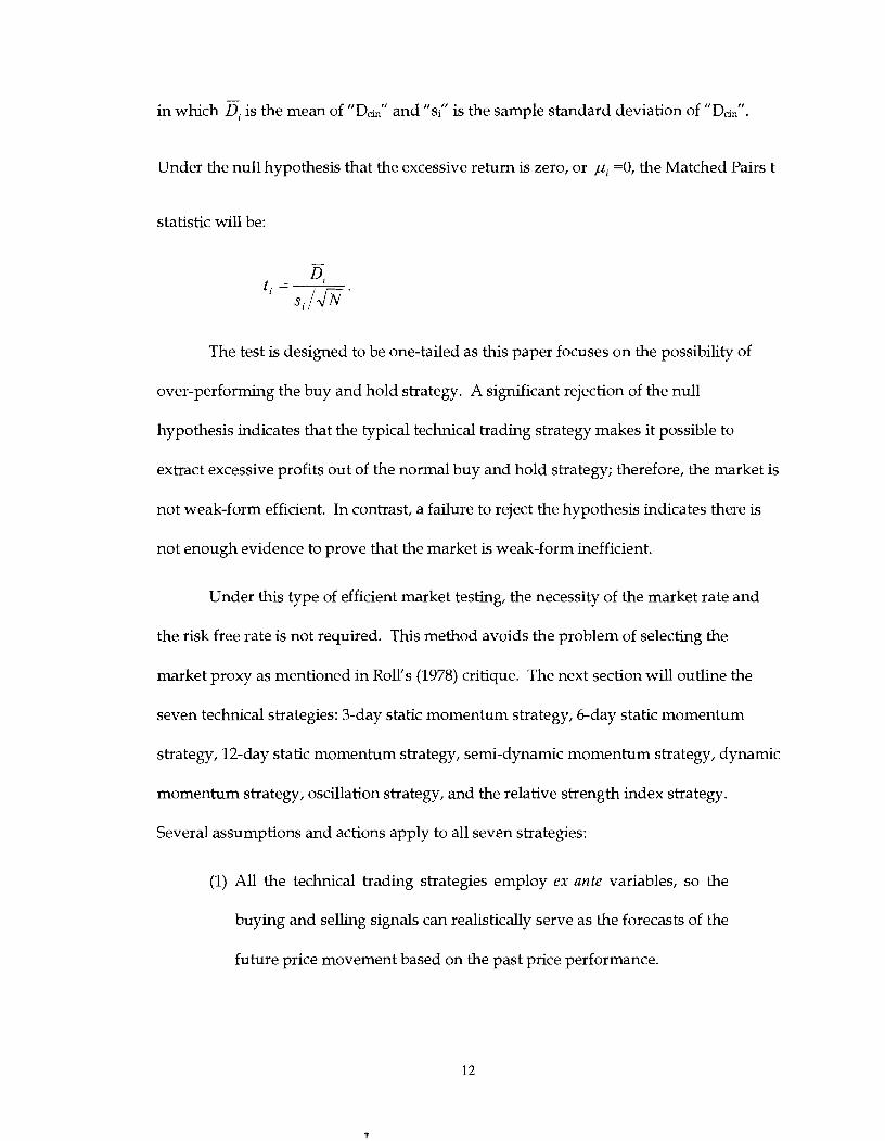
in which q. is the mean of "Dcin" and "si" is the sample standard deviation of "Dci/.
Under the null hypothesis that the excessive return is zero, or pi =0, the Matched Pairs t
statistic will be:
The test is designed to be one-tailed as this paper focuses on the possibility of
over-performing the buy and hold strategy. A significant rejection of the null
hypothesis indicates that the typical technical trading strategy makes it possible to
extract excessive profits out of the normal buy and hold strategy; therefore, the market is
not weak-form efficient. In contrast, a failure to reject the hypothesis indicates there is
not enough evidence to prove that the market is weak-form inefficient.
Under this type of efficient market testing, the necessity of the market rate and
the risk free rate is not required. This method avoids the problem of selecting the
market proxy as mentioned in Roll's (1978) critique. The next section will outline the
seven technical strategies: 3-day static momentum strategy, 6-day static momentum
strategy, 12-day static momentum strategy, semi-dynamic momentum strategy, dynamic
momentum strategy, oscillation strategy, and the relative strength index strategy.
Several assumptions and actions apply to all seven strategies:
(1) All the technical trading strategies employ ex ante variables, so the
buying and selling signals can realistically serve as the forecasts of the
future price movement based on the past price performance.

(2) To avoid time lag, the buy and sell actions are implemented immediately
when the signals appear. Realistically, if the reference price is the close price,
the confirmation of the signal takes time 1 minute before the close, and the
actual buy action is executed at the last minute. This action is superior to the
buy/sell at the open price as the price difference between the close and the
next open could be substantially large.
(3) The distribution of the security return is assumed to be log-normal; and the
daily security difference is assumed to be normally distributed.
3.1 Static Momentum Strategy
As the name suggests, static momentum strategies stem from the momentum
anomaly. It is based on the belief that the price persists over time. All of the static
momentum strateges in this paper embed the following four propositions:
(1) The word "static" describes the circumstance that the buy signals and
the sell signals do not respond to the qualitative price movements.
The static momentum strategy is based on the belief that stock price
movements are persistent in the "direction" of the change, and not in
the "performance" of the price change.
(2) The number "n" in the "n-day static momentum strategy" refers to
the observation period. This strategy supposes that the buy signals
appear when at least 67% of the observation days' returns are
positive. For instance, in the Sday static momentum strategy, the buy
signals appear when at least 2 days' returns out of 3 days are positive.

As a result, two initiative buy signal are generated at "n" when (n-2,
n-1,n) is (-,+,+) and (+,-,+).
(3) The holding period for each buy signal is 3 days.
(4) Continual update of the buy signals applies. Take an example when the
return for the past 9 periods (n-8,n-7,n-6,n-5,n-4,n-3,n-2,n-I,n) is (-,-,+,+,+,+,-,-
,+); if the observation period is 6 days, then the initial buy action will take
time at the close of "n-3" and hold until the end at "n". Nevertheless, the buy
signal is still active at "n," as the returns of 4 days out of 6 are positive, the
hold will continue at "n" until the signal is off at "n+3", "n+6", etc.
3.1.1 3-Day Static Momentum Strategy
The 3-day static momentum stresses the belief that momentum occurs in the
fairly short term, around a week. This strategy will automatically buy the stock when
the past return at (n-2,n-1,n) is (-,+,+) and (+,-,+); and will continue to hold when the
return is (+,+,-).
3.1.2 6-Day Static Momentum Strategy
The 6-day static momentum, compared to the 3-day one, is a bit conservative and
requires 6 days of observation before entering a trade. The buy actions take place when
at least 4 days' returns out of 6 days are positive. The holding period is still 3 days. As
result, the trade frequency will be smaller.

3.1.3 12-Day Static Momentum Strategy
The 12-day static momentum, compared to the other two, is the most
conservative as it searches for signs in the past 12 days and holds the security for only 3
days. The buy actions take place when at least 8 days' returns out of 12 days are
positive.
3.2 Semi-Dynamic Momentum Strategy
One of the salient shortcomings of the pure static strategy is the lack of
consideration of the performance measure. The semi-dynamic momentum strategy
eliminates this deficiency by implementing magnitude-sensitive buy signals. It is
"dynamic" as the buy signals can change. However, the holding period remains 3 days,
so it is semi-dynamic.
The buy signals are formed through statistical process. In general, the buy signal
is generated when:
* DD,, 2 PC, + t I-a,~-l , l X
in which "DDC," is the daily difference of the security price of country "c" at time "nu;
" N is the number of observation days; " p,, " is the mean of the DDcn for the past " N
observation days; " " is the standard error of the DDcn for the past "N"
observation days; and " t*l-a,~-~,l'l is the critical t value for 1-alpha confident, N-1
degrees of freedom, and one-tailed test. As the general model of buy signal is formed,
the next step will be to quantify the variables used in the paper:
(1) The DD,, will be the security price at "n" minus the security price at "n-1".
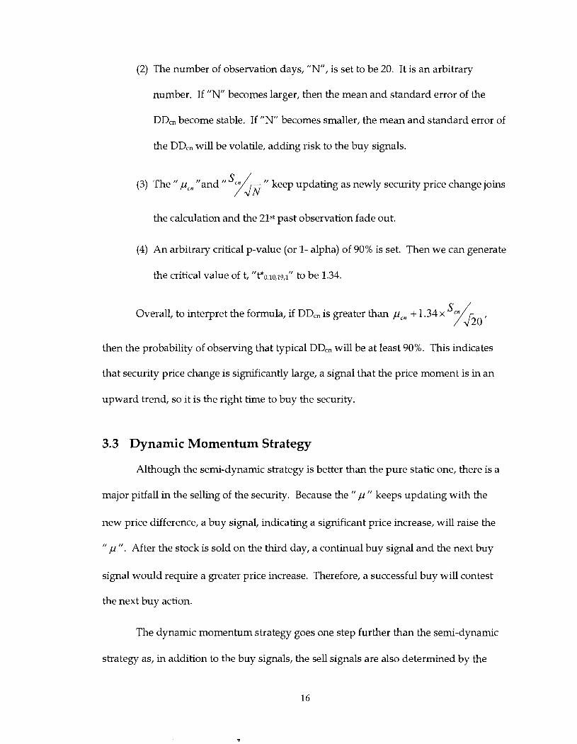
(2) The number of observation days, "Nu, is set to be 20. It is an arbitrary
number. If " N becomes larger, then the mean and standard error of the
DDc, become stable. If " N becomes smaller, the mean and standard error of
the DDcn will be volatile, adding risk to the buy signals.
(3) The " p,, "and " " keep updating as newly security price change joins
the calculation and the 215t past observation fade out.
(4) An arbitrary critical p-value (or 1- alpha) of 90% is set. Then we can generate
the critical value of t, "~*o.Io,I~,I~' to be 1.34.
Overall, to interpret the formula, if DDcn is greater than pCn + 1.34 x Sfm,
then the probability of observing that typical DDc, will be at least 90%. This indicates
that security price change is sigruficantly large, a signal that the price moment is in an
upward trend, so it is the right time to buy the security.
3.3 Dynamic Momentum Strategy
Although the semi-dynamic strategy is better than the pure static one, there is a
major pitfall in the selling of the security. Because the " p " keeps updating with the
new price difference, a buy signal, indicating a sigruficant price increase, will raise the
" p ". After the stock is sold on the third day, a continual buy signal and the next buy
signal would require a greater price increase. Therefore, a successful buy will contest
the next buy action.
The dynamic momentum strategy goes one step further than the semi-dynamic
strategy as, in addition to the buy signals, the sell signals are also determined by the

security performance. It is fully dynamic as both the buy signals and sell signals can
change. The buy signals are exactly identical to the buy signal of the semi-dynamic
strategy. On the other hand, the sell signals are triggered when:
The formula and the notations are the same as in the semi-dynamic strategy buy signal,
except the inequality sign and the critical p-value. In this paper, an arbitrary critical p-
value (or alpha) of 16% is used. Then the critical value of t, "t*0.16,19,1~~ will be -1.00.
The overall interpretation will be that if daily difference of the security price is
smaller than p,, - 1 .OO x '/$ (or price loss is greater than p, - 1 .OO x in
absolute term), then the probability of observing that typical DDcn will be at most 16%.
This indicates that security price change is sigruficantly small (the price loss is
significantly large), a signal that the price upward moment ends, so it is the right time to
sell the security.
3.4 Oscillation Strategy
According to Poitras (2005) "the term oscillator refers to a wide range of
techniques that can be based on substantively different calculations and motivations.
The unifying notion connecting the techniques is that the chart pattern calculated from
the original price chart oscillates or fluctuates within a defined range."
This paper will focus on the narrow definition found at www.futuresource.com
(2004) which defines an oscillator as "the simple difference between two moving
averages". A specific form is the dual exponential moving average. Generally, two
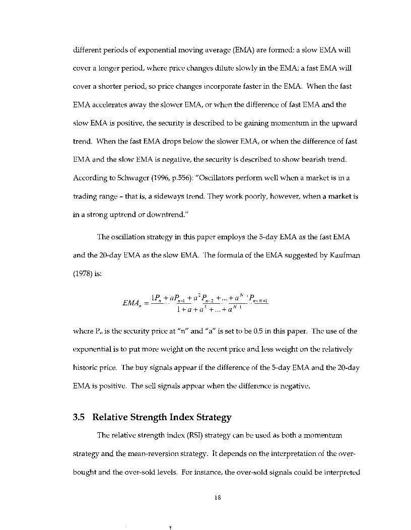
different periods of exponential moving average (EMA) are formed: a slow EMA will
cover a longer period, where price changes dilute slowly in the EMA; a fast EMA will
cover a shorter period, so price changes incorporate faster in the EMA. When the fast
EMA accelerates away the slower EMA, or when the difference of fast EMA and the
slow EMA is positive, the security is described to be gaining momentum in the upward
trend. When the fast EMA drops below the slower EMA, or when the difference of fast
EMA and the slow EMA is negative, the security is described to show bearish trend.
According to Schwager (1996, p.556): "Oscillators perform well when a market is in a
trading range - that is, a sideways trend. They work poorly, however, when a market is
in a strong uptrend or downtrend."
The oscillation strategy in this paper employs the 5-day EMA as the fast EMA
and the 20-day EMA as the slow EMA. The formula of the EMA suggested by Kaufman
(1978) is:
lP, +a<-, +a2%-, +. . .+aN- '~n-N+I EMA, =
1 + a + a 2 +...+ aN-'
where P, is the security price at "n" and "a" is set to be 0.5 in this paper. The use of the
exponential is to put more weight on the recent price and less weight on the relatively
historic price. The buy signals appear if the difference of the 5-day EMA and the 20-day
EMA is positive. The sell signals appear when the difference is negative.
3.5 Relative Strength Index Strategy
The relative strength index (RSI) strategy can be used as both a momentum
strategy and the mean-reversion strategy. It depends on the interpretation of the over-
bought and the over-sold levels. For instance, the over-sold signals could be interpreted

as a situation where the security price is below its fundamental value and is expected to
go back to the fundamental level. On the other hand, the over-sold signals could be a
signal of subsequent price fall. This paper will interpret the RSI as the mean-reversion
strategy. Nevertheless, as the returns in this paper are expressed as log return,
multiplying the RSI returns by a factor of negative one could shift the results from
mean-reversion strategy to momentum strategy1.
According to Schwager (1996, p542), "RSI compares the relative strength of price
gains on days that close above the previous day's close to price losses on days that close
below the previous day's close." The process of calculating the relative strength index is
detailed as follows:
(1) The RSI can be constructed with any number of observation days; a 9-day
period is used in this paper. A shorter observation period induces faster and
a more sensitive indicator, and vice versa.
(2) An up average is formed by adding all the prices gained on the up days of
the 9-day period and dividing the total by nine.
(3) A down average is formed by adding all the absolute values of the prices lost
on the down days of the 9-day period and dividing the total by nine.
(4) A relative strength (RS) can be calculated by dividing the up average by the
down average.
(5) The following formula will lead to the RSI:
RSI = 100 - [lo% + RSl]
1 Substantial difference may occur as the alternative strategy would involve short-selling.

An over-sold signal occurs when the RSI is very small. As down average
dominates the up average, O<RS<l, so RSI will be smaller than 50. Inversely, an over-
bought signal will result in a high RSI, 50<RSI<100. Since we interpret the RSI strategy
as a mean-reversion strategy, the over-sold signals will be the buy signals and the over-
bought signals will be the sell signals. The over-sold signals usually range from 20 to 30
and the over-bought signals usually range form 70 to 80. This paper will arbitrarily pick
the combination of (20,80) respectively.
4 DATA
As we are now in the high cross-border investment era, global market efficiency
becomes more important. "If momentum exists globally, then a strategy that actively
allocates funds from loser to winner markets might be more attractive than a globally
diversified buy-and-hold strategy (Fong, Wong, and Lean, 2003)." This paper will
examine the global weak-form market efficiency by testing the technical strategy return
of 24 country indexes and 1 world index from the Morgan Stanley Capital International
(MSCI) World Index. The 24 country indexes consist of Australia, Austria, Belgium,
Canada, Denmark, Finland, France, Germany, Hong Kong, Indonesia, Italy, Japan,
Korea, Malaysia, Netherlands, Norway, Singapore, South Africa, Spain, Sweden,
Switzerland, Taiwan, Thailand, United Kingdom, and United States. All data are
sourced from Datastream.
"The MSCI World Index is a free float-adjusted market capitalization index that
is designed to measure global developed market equity performance (MSCI 2004)."

Every MSCI index comprises large capitalization stocks and actively traded stocks, so
the problems associated with illiquidity, bid-ask spreads, and non-synchronous trading
biases are eliminated. Local prices are used in the indexes, thus returns will not be
distorted by the exchange rate fluctuations.
The price indexes are listed daily and the sample ranges from January 1989 to
September 2004. Since only the daily closed price was provided, the daily return is
formulated by comparing today's close price to that of the previous day. Due to the
limitation of the data, a trade, following a signal, is assumed to be executed the moment
before the close. An important assumption would be that there is no time lapse between
the signal and the trade action.
5 RESULTS AND SUMMARY
5.1 Full Period Returns of the Technical Trade Strategies
Table 1 in Appendix reports the performance of all the technical trade strategies
and the buy and hold strategy for all the indexes through the whole 15 years sample
period. All the returns are calculated in log form and expressed annually.
5.1.1 The 3 Static Momentum Strategies
Of all the technical trading strategies, those 3 static momentum strategies are
comparable because their basics are the same and they only differ in the observation
period. Among them, the most successful is the 3-day observation; it over-performs the
buy and hold strategy for 15 out of 25 world indexes. There are only 10 over-

performances in the 6-day strategy and only 8 in the 12-day strategy. Austria,
Indonesia, Korea, Malaysia, Taiwan, and Thailand are the countries where all the static
momentum strateges succeed in beating the buy and hold. Most of them cluster in the
South East Asian region. Nevertheless, up to this point we cannot conclude that these
markets are inefficient because the buy and hold strategy only compare the prices of the
initial trading day and the last one. The Asia Financial Crisis could be the blame for all
of the static momentum strategies over-performance relative to the buy and hold.
In addition, no salient trend is discovered in the number of observation days.
Generally, as the observation period increases, the returns generally decrease, but there
are lots of exceptions, so we cannot conclude any trend. However, a surprise appears in
Japan as all 3 static momentum strategies result in negative returns. This could be
understandable as the Japanese economy underwent suppression throughout the 1990's.
Another surprise is found in the Netherlands and Spain; the returns are positive in 3-day
observation and 12-day observation, but negative in the 6-day observation. The
difference is quite high especially in Spain.
5.1.2 The Other 4 Technical Trading Strategies
We cannot cross-compare the semi-dynamic, the dynamic, the oscillation, and
the RSI strategies. However, we can generally describe their performance. Of all 7
strategies, the most successful one is the dynamic strategy as it over-performs the buy
and hold for 23 country indexes and 1 world index. The only exception is United States
(Please refer to table 2 in Appendix). The semi-dynamic over-performs in 16 indexes;
oscillation strategy over-performs in 10 indexes. The relative strength index strategy
does not over-perform in any index. The success in the dynamic strategy can be

attributed to its ability to customize the trade signals with regard to the index
performance. Under the dynamic strategy, we know that the return from Japan can be
positive with a more customized strategy.
Another interesting logic can be formed by comparing the semi-dynamic and the
dynamic strategies: the selling signal is as important as the buy signal. A customized
sell signal, as in the dynamic strategy, enhances the return in all indexes except Taiwan.
We can now move onto the test result of the strategies.
5.2 Return of All the Strategies Listed Yearly
Table 3 averages all the returns across the 25 global indexes and expresses them
year by year. Three distinctive observations are discovered:
During the periods of negative buy and hold return, all of the technical
trading strategies over-perform. It sigrufies that it is possible to filter the
losses during a year.
During the periods of moderate growth, some strategies over-perform and
some under-perform. It varies strategy by strategy.
During the periods of rapid growth, the technical strategies do not hammer
the buy and hold strategy. The momentum in the indexes during the period
is strong. An attempt to filter the anticipated losses inversely filters the
gains.
In conclusion, these technical trading strategies could be employed to hedge and
eliminate the negative market risk.

5.3 Test Result for the Static Momentum Strategy
5.3.1 Test Result of the 3-Day Static Momentum Strategy
Table 4 shows the result of the matched pair t statistic of the 3-day static
momentum strategy. Korea, Malaysia, Singapore, and Taiwan reject the null hypothesis
at 10% sigdicance; Canada, and Thailand reject it at 5% significance; in the extreme,
Indonesia rejects the weak-form efficiency hypothesis at 1 % significance. Most of these
countries are located in the South East Asian region. However, it is quite surprising that
Canada is weak-form inefficient under this test. In contrast, Canada's neighbour, United
States, shows the least excessive return. The 3-day static momentum strategy yields a
loss of 9.08% compared to the buy and hold strategy. In addition, the standard error is
2.26%, one of the lowest in the data; sigdying that the loss is consistent.
5.3.2 Test Result of the 6-Day Static Momentum Strategy
With the 6-day momentum strategy, only Indonesia, Korea, and Thailand are
proven to be weak-form market inefficient. The Result is reported in Table 5. This time,
again, the Indonesian market is proven to be weak-form inefficient. The excessive return
from this strategy is 17.42%, better than that of the 3-day static momentum strategy with
30.17%. The Netherlands and United States provide the least returns, -9.70% and -8.26 %
respectively.
5.3.3 Test Result of the 12-Day Static Momentum Strategy
Table 6 reports the test for the 12-day static momentum strategy. None of the
global markets is proven to be inefficient. Indeed, 17 out of the 25 markets show
negative excessive returns anchoring the buy and hold strategy. The excessive return in

Indonesia is actually larger than that in the 6-day static momentum strategy, but the
standard error is much larger. Belgium, France, Hong Kong, Switzerland, United
Kingdom, and United States report the least gain (most loss), but United Kingdom is
proven to be most efficient in this test.
5.4 Test Result for the Semi-Dynamic Momentum Strategy
Table 7 shows that the semi-dynamic momentum strategy beats the buy and hold
strategy in 9 country indexes and in the world index. The countries are Austria, Canada,
Hong Kong, Indonesia, Italy, Malaysia, Norway, South Africa, Taiwan, and Thailand.
On the other hand, Switzerland and the Netherlands are proven to be efficient under
this test.
5.5 Test Result for the Dynamic Momentum Strategy
The result generated from this dynamic momentum strategy can significantly
separate the inefficient market from the efficient ones. The result is shown in table 8.
German and United States markets are the most efficient under this test as they are the
only two that produce negative excessive returns. Of the remaining 23 indexes, 14
significantly produce positive excessive return. Austria, Canada, Hong Kong, Italy,
Korea, Malaysia, Norway, Singapore, South Africa, Spain, and Sweden are inefficient at
5% level. The world index, Indonesia, and Thailand are inefficient at 1 % level. The
excessive return in Indonesia and Thailand are 40.58 % and 35.46 % respectively.
Although the excessive return in the world index is only 13.28%, the standard error is
quite low, making it highly sigruficant. It is surprising that Taiwan, proven to be weak-
form market inefficient in the semi-dynamic strategy, appears to be efficient now.

Perhaps, the bearish sentiments in the Taiwanese market arrived promptly, leaving the
sell signals ineffective in exiting the market.
5.6 Test Result for the Oscillation Strategy
Table 9 shows the test result for the oscillation strategy. Only Indonesia, Korea,
Malaysia, and Thailand get significant excessive returns. Again, the Netherlands,
United Kingdom, and United States are proven efficient under this test.
5.7 Test Result for the Relative Strength Index Strategy
Table 10 reports the test result for the relative strength index (RSI) strategy. If we
interpret the RSI as a mean reversion indicator, then the result will show that all of the
global markets are efficient. Nevertheless, the negative of the mean-reversion (MR) RSI
strategy return is approximately equal to the return for the momentum (MM) RSI
strategy.
When: (MR-RSI Return) - (Buy and Hold Return) = (MR-Excessive Return),
given that: (MM-RSI Return) = - (MR-RSI Return) ,
it follows: (MM-Excessive Return) = - (MR-Excessive Return)
- 2(Buy and Hold Return).
This explains why the excessive return for Indonesia is extremely negative; as it
implies the high excessive return for the momentum RSI strategy. All in all, the low t-
stat for Indonesia, Malaysia, Singapore, Switzerland, and Thailand can be translated into
high t-stat under the momentum RSI strategy, indicating that markets are inefficient.
When none of the mean reversion RSI excessive returns is positive, one may Infer that

momentum anomaly dominates the mean reversion anomaly. However, further proof is
required.
6 DISCUSSION AND CONCLUSION
This paper investigates the global weak-form market efficiency through
selections of technical analysis including the static, semi-dynamic, and dynamic
momentum strategies, oscillation strategy, and the relative strength index strategy. As
long as one of the tests shows that the market is inefficient, then the market is inefficient
because it is possible to extract excessive profit based on technical analysis. Of the 24
country indexes and 1 world index, only 10 are proven to be efficient as there are
inadequate evidences to prove the existence of excessive profits beyond the buy and
hold strategy. These 10 countries are Australia, Belgium, Denmark, France, Germany,
Japan, Netherlands, Switzerland, United Kingdom, and United States. In the most
extreme, none of the technical strategies employed in this paper produces positive
excessive profits in United States and Germany. All of these countries are fully
developed, and so are their financial sectors. The technical traders in these countries
would have already swept the momentum and the mean-reversion anomaly, leaving no
room for excessive profit under the strategies in the paper. On the other hand, the most
sigruficant inefficient markets proven in this paper are Indonesia, Korea, Malaysia, and
Thailand. These countries are predominantly categorized as the "emerging markets";
inefficiency in their financial market is understandable. Through out the paper, Canada
is actually considered inefficient as sigruficant excessive profits can be extracted in 3 of

the 7 technical strategies. The physical distance of Canada and United States is very
close, but the market efficiency is widely apart.
This paper also discovered several properties of the trading strateges:
First of all, trends are not discovered in the static momentum strategy as the
number of observation days increase. The market characteristic in each
country disturbs the trend in the global basis.
The sell signals are as important as the buy signals. To illustrate, all the
market returns increases significantly from the semi-dynamic strategy to the
fully dynamic strategy, with the only exception of Taiwan.
A more customization of the strategies results in better return. For example,
dynamic strategy is better than the semi-dynamic one, which is also better
than the pure static momentum strategies.
Schwager's statement regarding oscillation does not coincide with the
evidence in this paper. He mentions that "[olscillators perform well when a
market is in a trading range - that is, a sideways trend. They work poorly,
however, when a market is in a strong uptrend or downtrend. (Schwager
1996, p.556)" Indonesia, Malaysia, and Thailand, are markets in very strong
uptrend or downtrend. However, their oscillation returns are the highest
among all.
However, another statement from Schwager found in this context regarding
the relative strength index strategy: "Traders should not automatically sell
markets that are over bought or buy markets that are oversold. Although

such a strategy may work well in a trading-range market, it will be
disastrous in a trending market. (Schwager 1996, p.524)" The mean-
reversion RSI strategy employed in t h s paper is based on the belief that an
over-sold market would revert as a winner and that an over-bought market
would revert as a loser. Indeed the returns in Indonesia, Malaysia, and
Thailand are drastically low. In strong trendy markets like them, over-
bought should be treated as buy signals and vice versa. The RSI strategy
should be best exploited as a momentum strategy.
The result also demonstrates that the technical trading strateges work the best
during the periods of negative market return and the periods of moderate growth. The
possibility to filter losses during the negative market return period makes the strateges
attractive for the fund managers trying to hedge their funds and minimizing downside
risks. It signifies that it is possible to filter the losses during a year. In addition, as t h s
paper demonstrates the sigruficance excessive profits, fund managers are encouraged to
diversify their investments country-wisely and maximize the portfolio value in the
inefficiency markets.
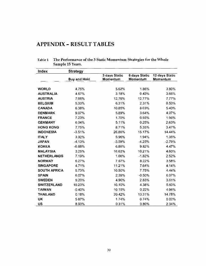
APPENDIX - RESULT TABLES
Table 1 The Performance of the 3 Static Momentum Strategies for the Whole Sample 15 Years.
Index Strategy 3 days Static 6 days Static 12 days Static
Buy and Hold Momentum Momentum Momentum
WORLD AUSTRALIA AUSTRIA BELGIUM CANADA DENMARK FRANCE GERMANY HONG KONG INDONESIA ITALY JAPAN KOREA MALAYSIA NETHERLANDS NORWAY SINGAPORE SOUTH AFRICA SPAIN SWEDEN SWITZERLAND TAIWAN THAILAND UK US
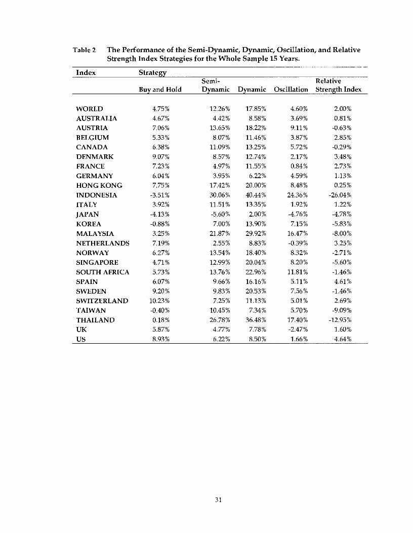
Table 2 T h e Performance of the Semi-Dynamic, Dynamic, Oscillation, a n d Relative Strength Index Strategies for t h e Whole Sample 15 Years.
Index
WORLD AUSTRALIA AUSTRIA BELGIUM CANADA DENMARK FRANCE GERMANY HONG KONG INDONESIA ITALY JAPAN KOREA MALAYSIA NETHERLANDS NORWAY SINGAPORE SOUTH AFRICA SPAIN SWEDEN SWITZERLAND TAIWAN THAILAND UK us
Strategy Semi- Relative
Buy and Hold Dynamic Dynamic Oscillation Strength Index
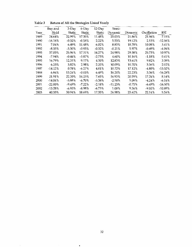
Table 3 Return of All the Strategies Listed Yearly
Year Buy and
Hold 3-Day Static
22.99% -0.32% 6.49%
-3.30% 25.96% -0.44% 12.31% 3.82% 0.78%
13.24% 22.30% -5.88% -9.49% -6.93% 30.94%
6-Day Static
17.35% -0.58% 11.48% -0.93% 17.31 % -3.87% 9.17% 2.98%
-6.27% -0.05% 14.23% -6.70% -7.22% -8.98% 18.69%
12-Day Static
11.48% 2.22% 6.02%
-0.32% 14.27% -2.73% 4.50% 2.55% 4.01 % 6.49% 7.65%
-5.38% -2.18% -6.73% 17.35%
Semi- Dynamic
25.03% 5.53% 8.85%
-0.21 % 24.98% 4.60%
12.83% 10.09% 10.72% 16.20% 16.93% -2.58%
-11.23% 1.08%
26.98%
Dynamic 21.86% 19.12% 18.78% 5.97%
29.38% 10.16% 13.61 % 10.70% 17.12% 22.23% 20.59% 5.09%
-0.75% 9.36%
23.62%
Oscillation RSI 21.98% 7.15% 2.13% -12.16%
10.08% 3.41% -0.49% -4.04% 25.73% 10.97% -1.18% 0.41% 9.82% 3.59% 3.56% 2.02%
-4.80% -15.52% 3.36% -16.28%
17.24% 8.14% -4.24% -6.14% -6.49% -16.50% -9.10% -10.89% 22.14% 5.56%
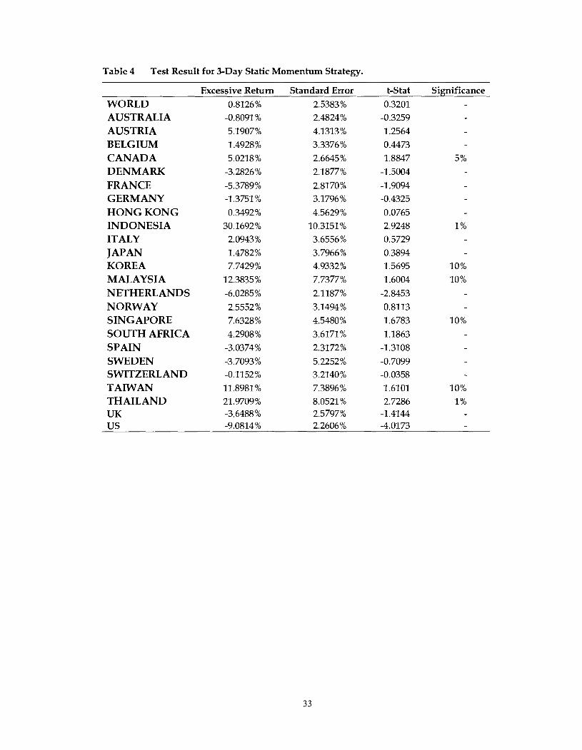
Table 4 Test Result for 3-Day Static Momentum Strategy.
Excessive Return WORLD 0.8126%
AUSTRALIA -0.8091 %
AUSTRIA 5.1907%
BELGIUM 1.4928 %
CANADA 5.0218%
DENMARK -3.2826%
FRANCE -5.3789% GERMANY -1.3751 %
HONG KONG 0.3492% INDONESIA 30.1692% ITALY 2.0943%
JAPAN 1.4782% KOREA 7.7429%
MALAYSIA 12.3835%
NETHERLANDS -6.0285%
NORWAY 2.5552%
SINGAPORE 7.6328%
SOUTH AFRICA 4.2908%
SPAIN -3.0374%
SWEDEN -3.7093% SWITZERLAND -0.1152%
TAIWAN 11.8981 % THAILAND 21.9709% UK -3.6488% US -9.0814%
Standard Error 2.5383% 2.4824%
4.1313% 3.3376%
2.6645%
2.1877%
2.8170% 3.1796%
4.5629% 10.3151% 3.6556%
3.7966% 4.9332 %
7.7377%
2.1187%
3.1494%
4.5480%
3.6171%
2.3172%
5.2252% 3.2140%
7.3896% 8.0521 % 2.5797% 2.2606%
Significance
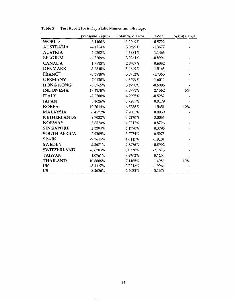
Table 5 Test Result for 6-Day Static Momentum Strategy.
Excessive Return Standard Error WORLD AUSTRALIA AUSTRIA BELGIUM CANADA DENMARK FRANCE GERMANY HONG KONG INDONESIA ITALY JAPAN KOREA MALAYSIA NETHERLANDS NORWAY SINGAPORE SOUTH AFRICA SPAIN SWEDEN SWITZERLAND TAIWAN THAILAND UK us
Significance
5%
10%
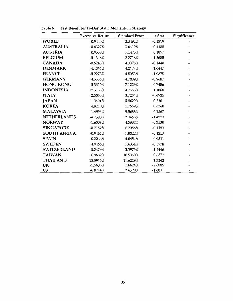
Table 6 Test Result for 12-Day Static Momentum Strategy
WORLD AUSTRALIA AUSTRIA BELGIUM CANADA DENMARK FRANCE GERMANY HONG KONG INDONESIA ITALY JAPAN KOREA MALAYSIA NETHERLANDS NORWAY SINGAPORE SOUTH AFRICA SPAIN SWEDEN SWITZERLAND TAIWAN THAILAND UK us
Excessive Return
-0.9440% -0.4327%
0.9558%
-5.1318%
-0.6245% -4.4064%
-5.2273 % -4.5536%
-5.3319%
17.5135% -2.5053%
1.3491 %
4.8210%
1.4996 %
-4.7598% -1.6003%
-0.7152%
-0.9461 % 0.2066%
-4.9466% -5.2479 %
6.9632% 15.3915% -5.5603% -6.8714%
Standard Error
3.3492% 3.6419%
5.1473%
3.2718% 4.3376%
4.2178% 4.8053%
4.7009% 7.1229%
14.7563% 3.7254%
5.8629%
5.7669%
9.5683%
3.3466% 4.5332%
6.2058%
7.8022%
4.0454%
5.6354% 3.3975%
10.5960%
11.6229% 2.6624% 3.6529%
t-Stat Significance
-0.2819 -0.1188
0.1857 -
-1.5685 -0.1440
-1.0447 -1.0878
-0.9687 -0.7486
1.1868 -0.6725
0.2301
0.8360
0.1567
-1.4223 -0.3530
-0.1153
-0.1213
0.0511
-0.8778 -1.5446
0.6572 1.3242
-2.0885 -1.8811
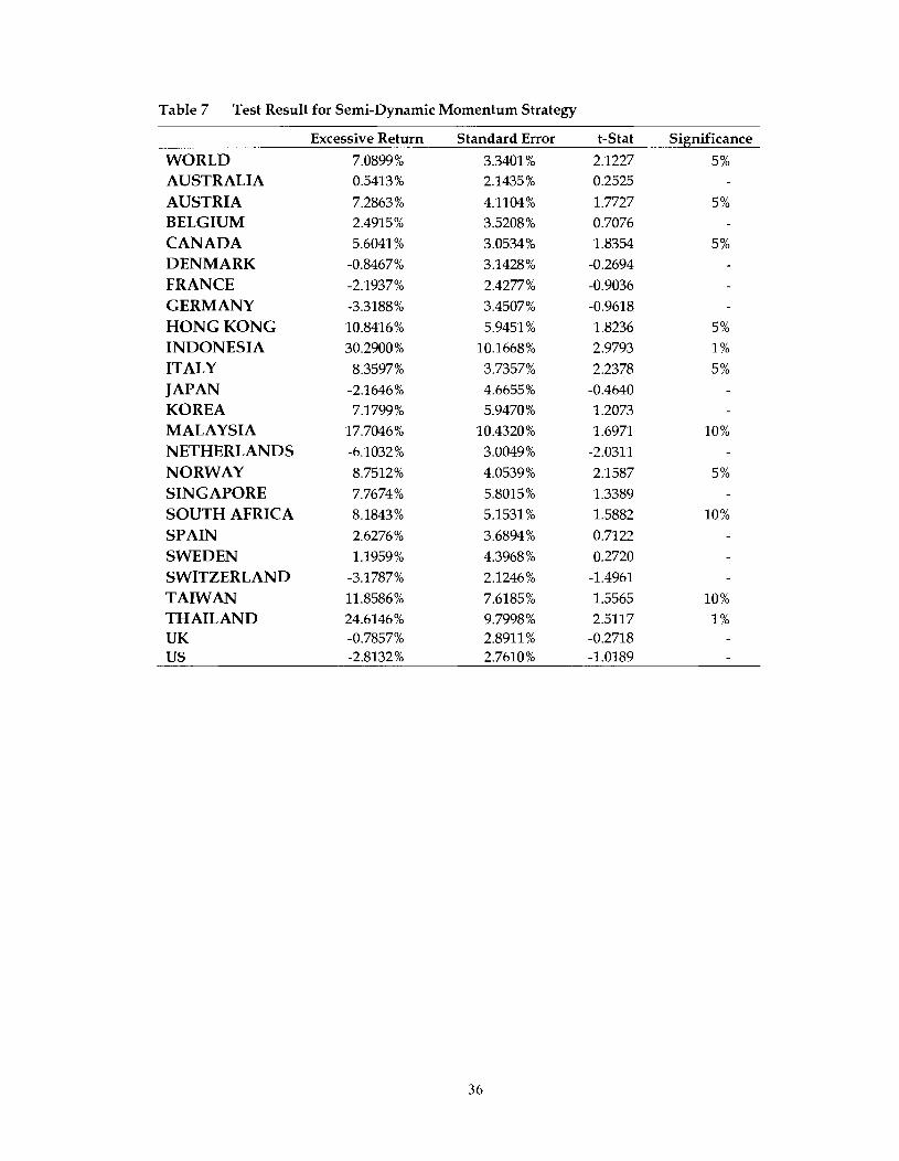
Table 7 Test Result for Semi-Dynamic Momentum Strategy
Excessive Return Standard Error Significance
WORLD AUSTRALIA AUSTRIA BELGIUM CANADA DENMARK FRANCE GERMANY HONG KONG INDONESIA ITALY JAPAN KOREA MALAYSIA NETHERLANDS NORWAY SINGAPORE SOUTH AFRICA SPAIN SWEDEN SWITZERLAND TAIWAN THAILAND UK us
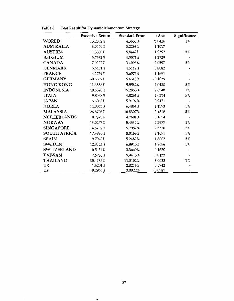
Table 8 Test Result for Dynamic Momentum Strategy
WORLD AUSTRALIA AUSTRIA BELGIUM CANADA DENMARK FRANCE GERMANY HONG KONG INDONESIA ITALY JAPAN KOREA MALAYSIA NETHERLANDS NORWAY SINGAPORE SOUTH AFRICA SPAIN SWEDEN SWITZERLAND TAIWAN THAILAND UK us
Excessive Return Standard Error
13.2832% 4.3658% 3.5549% 3.2266%
11.3330% 5.8442%
t-Stat Significance
3.0426 1% 1.1017
1 .9392 5%
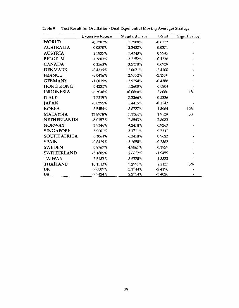
Table 9 Test Result for Oscillation (Dual Exponential Moving Average) Strategy
Excessive Return
WORLD AUSTRALIA AUSTRIA BELGIUM CANADA DENMARK FRANCE GERMANY HONG KONG INDONESIA ITALY JAPAN KOREA MALAYSIA NETHERLANDS NORWAY SINGAPORE SOUTH AFRICA SPAIN SWEDEN SWITZERLAND TAIWAN THAILAND UK us
Standard Error
2.2508% 2.3422%
3.4243% 3.2252% 3.5178% 2.6631 %
2.7752%
3.9294% 5.2600%
10.0860% 3.2266% 5.4419%
5.6727% 7.1164% 2.8543% 4.2478% 5.1721 % 6.3458% 3.2650% 4.9867%
2.6623% 5.6370% 7.2995% 3.1744% 2.2754%
Significance -
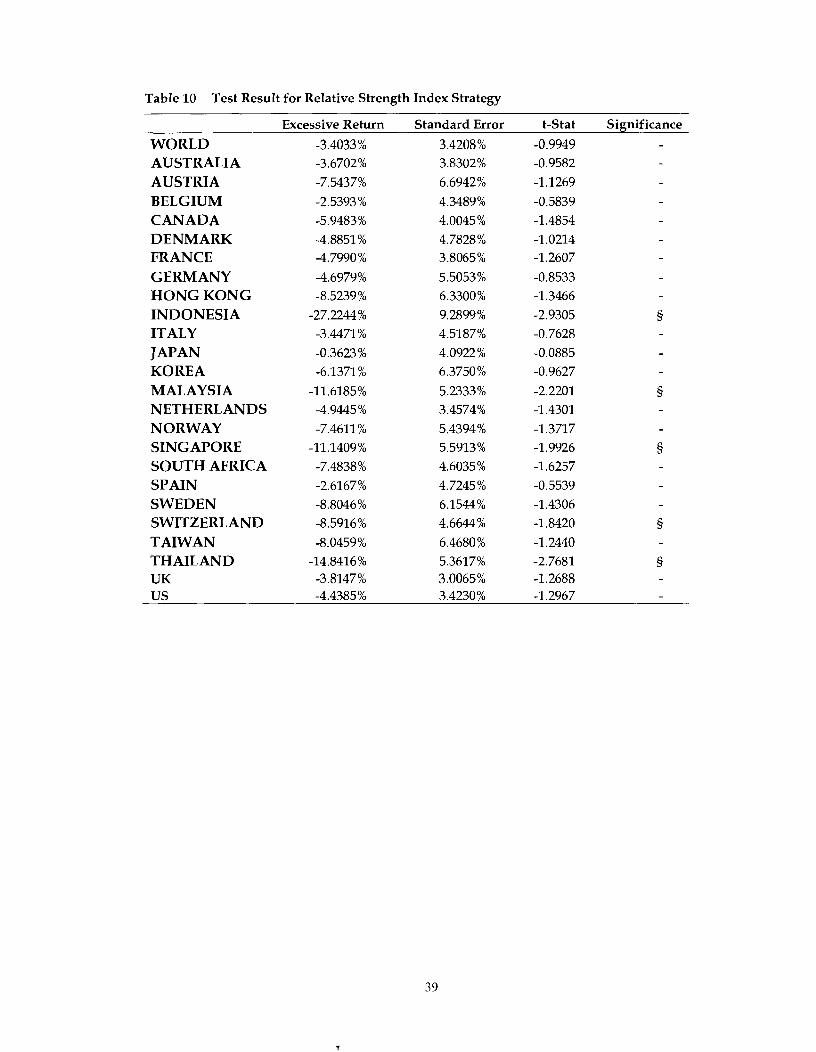
Table 10 Test Result for Relative Strength Index Strategy
Excessive Return Standard Error t-Stat Significance
WORLD AUSTRALIA AUSTRIA BELGIUM CANADA DENMARK FRANCE GERMANY HONG KONG INDONESIA ITALY JAPAN KOREA MALAYSIA NETHERLANDS NORWAY SINGAPORE SOUTH AFRICA SPAIN SWEDEN SWITZERLAND TAIWAN THAILAND UK
REFERENCE LIST
Barberis, Nicholas, Andrei Shleifer, and Robert Vishny. 1998. A Model of Investor Sentiment. Journal of Financial Economics 49, 307-343.
Berk, Jonathan B., Richard C. Green, and V. Naik. October 1999. Optimal
Investment, Growth Options, and Security Returns. The Journal of Finance
LIV, no. 5.
Boudoukh, J., M. Richardson, and R. Whitelaw. 1994. A Tale of Three Schools:
Insights on Auto-Correlations of Short-Horizon Stock Returns. Review of
Financial Studies 7,539-573.
Chan, K. C. 1988. On the Contrarian Investment Strategy. Journal of Business 61,
no. 2.
Chopra, N., J. Lakonishok, and J. R. Ritter. 1992. Measuring abnormal
performance: Do stocks overreact? The Journal of Financial Economics 31,235-
268.
Chordia, Tarun, and Lakshmanan Shivakumar. April 2002. Momentum, Business Cycle, and Time-varying Expected The Journal of Finance LVII, no. 2.
Conrad, Jennifer, and Gautam Kaul. Autumn 1998. An Anatomy of Trading
Strategies. The Reoiew of Finnncial Studies 11, no. 3:489-519.
Conrad, Jennifer, and Gautam Kaul. 1989. Mean Reversion in Short-Horizon
Expected Return. The Review of Financial Studies 2, no. 2:225-240.
Constantinides, G. 1984. Optimal Stock Trading With Personal Taxes. The Journal of Finnncial Eocnomics 13,65-89.
Daniel, Kent, David Hirshleifer, and Avanidhar Subrahmanyam. December 1998.
Investor Psychology and Security Market Under- and Overreactions. The
Journal of Finance LIII, no. 6.

De Bondt, Werner F. M., and Richard Thaler. July 1985. Does the Stock Market Overreact? The Journal of Finance XI, no. 3.
De Bondt, Werner F. M., and Richard H. Thaler. July 1987. Further Evidence On
Investor Overreaction and Stock Market Seasonality. The Journal of Finance
XLII, no. 3.
Edwards, W. 1968. Conservatism in Human Information Processing. In Formal
Representation of Human Judgment, edited by B. Kleinmutz. New York: John
Wiley and Sons.
eSignal. 2004. Futuresource.com. [database online] Illinois, United States.
Available from http://www.futuresource.com/reference/studies.jsp?
study=OSC. Dec 1,2004.
Fama, E. F., and K. R. French. 1988a. The Journal of Political Economy.
Permanent and Temporary Components of Stock Prices. 96,246-273.
Fama, E. F., and K. R. French. 1987. Commodity Futures Prices: Some Evidence on Forecast Power, Premiums, and the Theory of Storage. Tlze Journal of
Business 60,55-73.
Fama, E. F., and K. R. French. 1996. Multifactor Explanations of Asset Pricing
Anomalies. The Journal of Finance 51/55-84.
Fama, Eugene F. 1970. Efficient Capital Markets: A Review of Theory and Empirical Work. The Journal of Finance 25,383-417.
Fischer, J. 1999. "Window Dressing". Rule Breaker Porffolio. Available from
http:/ / www.fool.com/ portfolio/rulebreaker/ 1999/ rulebreaker991004.htm
December 1,2004.
Fong, Wai M., Wing K. Wong, and Hooi H. Lean. August 2003. International
Momentum Strategies: A Stochastic Dominance Approach. University of
Singapore.
French, Kenneth. 1980. Stock Returns and the Weekend Effect. Journal of Financial
Economics 8/55-69.
Grinblatt, M., and T. J. Moskowitz. 2003. Predicting Stock Price Movements from Past Returns: The Role of Consistency and Tax-Loss Selling". Journal of
Financial Economics.
Grinblatt, Mark, Sheridan Titman, and Russ Wermers. December 1995.
Momentum Investment Strategies, Portfolio Performance, and Herding: A Study of Mutual Fund Behavior. The American Economic Reviezu 85, no.
5:1087-1105.
Grundy, B.D., and J.S. Martin. 2001. Understanding the Nature of the Risks and
the Source of the Rewards to Momentum Investing. Review of Financial
Studies 14/29-78.
Hong, Harrison, Terence Lim, and Jeremy C. Stein. February 2000. Bad News
Travels Slowly: Size, Analyst Coverage, and the Profitability of Momentum
Strategies. The Journal of Finance LV, no. 1.
Hong, Harrison, and Jeremy C. Stein. December 1999. A Unified Theory of
Underreaction, Momentum Trading, and Overreaction in Asset Markets. The
Journal of Finance LIV, no. 6.
Jegadeesh, Narasimhan. July 1990. Evidence of Predictable Behavior of Security
Returns. The Journal of Finance XLV, no. 3.
Jegadeesh, Narasimhan, and Sheridan Titman. March 1993. Returns to Buying
Winners and Selling Losers: Implications for Stock Market Efficiency. The
Journal of Finance XLVIII, no. 1.
Kahneman, Daniel, and Amos Tversky. 1984. Choices, Values and Frames.
American Psychologist, 39,341-350.
Kaufman, Perry J. 1978. Commodity Trading Systems and Methods. Canada: John
Wiley & Sons, Inc.
Kaul, G., and M. Nimalendran. 1990. Price Reversals: Bid-Ask Errors or Market
Overreaction? lournal of Financial Economics 28/67-93.

Lakonishok, Josef, Andrei Shleifer, and Robert W. Vishny . 1994. Contrarian Investment, Extrapolation, and Risk. The Journal of Finance. Vol. 49, Iss. 5: p.
1541
Lee, Charles M. C., and Bhaskaran Swaminathan. October 2000. Price
Momentum and Trading Volume. The Journal of Finance 55, no. 5:2017-2069.
Lehmann, B. N. 1990. Fads, Martingales, and Market Efficiency. Quarterly Journal of Economics 105,l-28.
Lo, Andrew W., and A. C. MacKinlay. 1988. Stock Market Prices Do Not Follow
Random Walks: Evidence from a Simple Specification Test. The Review of Financial Studies 1, no. 2:41-66.
Moore, David S. 1995. The Basic Practice of Statistics. United States of America: W. H. Freeman and Company.
Morgan Stanley Capital International Inc. 2004. Morgan Stanley Capital International Equity Indices. [database online]. New York, Available from
http:/ /www.msci.com/overview/index.html. September 29,2004.
Poitras, Geoffrey. 2005. Security Analysis and Investment Strategy. Oxford, United Kingdom: Blackwell Publishing.
Roll, Richard. 1978. Ambiguity when Performance is Measured by the Securities
Market Line. Journal of Finance 33,1051-1069.
Scholes, M., and J. T. Williams. 1977. Estimating Betas from Nonsynchronous
Data. Journal of Financial Economics 5,309-327.
Schwager, Jack D. 1996. Technical Analysis. Edited by Jack D. Schwager. Canada:
John Wiley & Sons, Inc.
Thaler, Richard. 1987. The Janurary Effect. Journal of Economic Perspectives 1,197- 201.
Thaler, Richard. 1987. Seasonal Movements in Securities Prices 11: Weekend, Holiday, Turn of the Month, and Intraday Effects. Journal of Economic
Perspectives 1,169-177.
Tversky, A., and D. Kahneman. 1974. Judgment Under Uncertainty: Heuristics
and Biases. Science 185,1124-1131.
Watkins, B. 2002. Does consistency predict returns? Unpublished zuorking paper. Syracuse University.
Zarowin, Paul. December 1989. Does the Stock Market Overreact to Corporate
Earnings Information? The Journal of Finance 44, no. 5:1385-1399.