Terms of Trade, Business Cycles and Tobin’s q in

Developing Open Economies

Víctor Pacharoni

April 15, 2004

! " # $

% &'( $ $ % ! % $ $ % !

)*+,-./0,121 32456,72 1. 35/1582 9/:.+4,+2; <=2,6> -,745/?@A775/;.1A2/

1

1 Introduction

In the Real Business Cycle (RBC) approach to developing open economics, large andrecurrent fluctuations in terms of trade are widely viewed as an important drivingforce of business cycles. The terms of trade affect the industrial countries mainlyby raising the relative price of energy. In developing countries this effect primarilyaffects the price of imported capital goods.

There is high volatility in the share markets of emerging economies over the longterm. In the beginning of the 90’s, RBC models for developing countries did notfocus on the share market, given that the size of the market was small. A comparisonof these series during the last decade shows that the stock market capitalization fordeveloping countries has greatly increased in their value relative to GDP.

Tobin’s q is used to account for the price of replacement of the capital. Tobin’sq is the ratio of the market value of an additional unit of capital to its replacementcost. Hayashi (1982) shows that the average and the marginal values of capitalare identical under neoclassical assumptions. Tobin and Brainard (1977) conjecturethat the average and marginal values respond in similar ways to shocks, and theempirical evidence in Abel and Blanchard (1986) appears to support the conjecture.The stock market indices are the value for the Tobin’s q used in this research.

This paper links stock market dynamics and the RBC model for developing

2

countries. As usual in RBC literature, we focus on volatility, correlation, and cross-correlation between the series in the real data and compare these with the statisticsfrom data generated by the model.

This paper addresses the following questions:- Do the dynamics of share prices for RBC correspond to the dynamics and

values for the stock market indices for a group of developing countries?- How much of the variability of changes in GDP and stock market indices are

implied by the terms of trade shocks?To answer these questions this paper does an examination of the relationship

between terms of trade shocks and business cycles from the perspective of a dynamicstochastic general equilibrium framework. It borrows numerical solution methodsfrom real business cycle theory to compute stochastic processes of three sector inter-temporal model of a small open economy. It compares various features of the model’sbusiness cycles with actual business cycles.

This paper extends Mendoza (1995) with an analysis of Tobin’s q. The paperdoes not use the endogenous discount factor; it is an exogenous variable. Thedata set is characterized by different frequencies, time and countries. This studyuses different numerical algorithms to find the solution, and incorporates a richersequence of the shocks.

This study follows Obstfeld and Roggff (1996) and Romer (1996) to introduce

3

the Tobin’s q theory and its implication. Both text books present the simplestsituation with only one capital and one good in a partial equilibrium model in theproduction side. The model used here is a general equilibrium model, and the valueof q is affected by the consumer preferences in each period.

To solve the model, this study follows Duffy and McNelis (2001). For assuringaccuracy in the simulations, it uses the Den Haan and Marcet (1994) statistic. Thisstudy also uses two different techniques: the linear quadratic approximation method,and parameterized expectations algorithm, with a neural network approach. Itsupports a complex combination of the state variables. The second algorithm helpsus to approximate the volatility of Tobin’s q for developing economies.

The paper has the following order: the next section analyzes the real side ofthe economy and shows the empirical regularities and some of the stylized facts.Section three develops the model and some of its variations and the equilibriumand dynamics of the economy. The steady state and parameters are presented insection four. Section five is a presentation of both solution algorithms. Benchmarksimulations are in section six. Section seven examines the robustness of the model.The last section concludes.

4

2 Empirical Regularities

This section studies key properties of the data, for Gross Domestic Product (GDP),Stock Market Indices (SMI), and Terms of Trade (TOT) , and their relations.

Data come from three different sources for each country. The First is fromThe World Bank, World Development Indicators (2001), series of Stock MarketCapitalization are from this database.

The Second is The International Financial Statistics (IFS), CD-Rom, December2001, for the series of GDP, of export prices (Px) and import prices (Pm). Theseries of TOT is a simple construction based on this data. The data are in constantUS dollars.

The other database is from Morgan Stanley Capital International (MSCI); thisdatabase is available from 1970 but not for all countries. This paper constructsseries of stock market indices, SMI, using the values of the last day of informationfor each quarter and this data comes in index values.

This research is limited by two restrictions: the first is the large amount of seriesto consider in this sample, the second is the amount of the countries.

The sample is between 1990 and 2000, for most of the countries. But a fewcountries have fewer observations. They are: Belgium, Singapore and Thailand,that begin in 1993; Argentina that finishes in 1998, and Poland that begins in 1995.

5

All off these limitations are due to missing data.The number of the countries is limited to 24. Some of them are not developing

economies; they serve as a comparison.These countries were put in three different groups: group of seven largest in-

dustrialized countries (G7), others industrialized countries (IC’s), and developingcountries (DC’s).

The list of the countries is:G7: Canada, France, Germany, Italy, Japan, United Kingdom, and United

States.IC’s: Australia, Belgium, Denmark, Finland, Netherlands, Norway, Sweden, and

Switzerland.DC’s: Argentina, Brazil, Hong Kong, Korea, New Zealand, Poland, Singapore,

Thailand, and Turkey.

6

Table 1:$ Millons

1990 1999 1990 1999

Canada 241,920 800,914 42.2 126.1France 314,384 1,475,457 25.9 103.0Germany 355,073 1,432,190 22.2 67.8Italy 148,766 728,273 13.5 62.2Japan 2,917,679 4,546,937 98.2 104.6United Kingdom 848,866 2,933,280 85.9 203.4United States 3,059,434 16,635,114 53.2 181.8mean 1,126,589 4,078,881 48.7 121.3

Australia 108,879 427,683 35.1 105.9Belgium 65,449 184,942 33.1 74.5Denmark 39,063 105,293 29.3 60.4Finland 22,721 349,409 16.6 269.5Netherlands 119,825 695,209 40.5 176.6Norway 26,130 63,696 22.6 41.6Sweden 97,929 373,278 41.2 156.4Switzerland 160,044 693,127 70.1 268.1mean 80,005 361,580 36.1 144.1

Argentina 3,268 166,068 2.3 29.6Brazil 16,354 226,152 3.5 30.3Hong Kong 83,397 609,090 111.5 383.2Korea, Rep. 110,594 148,649 43.8 75.8New Zealand 8,835 28,352 20.5 51.9Poland 144 31,279 0.2 19.1Singapore 34,308 198,407 93.6 233.6Thailand 23,896 29,489 28.0 46.9Turkey 19,065 69,659 12.6 60.7mean 33,318 167,461 35.1 103.5

Chile 13,645 60,401 45.0 101.1Mexico 32,725 125,204 12.5 31.8Peru 812 10,562 3.1 25.8Israel 3,324 64,081 6.3 63.3Saudi Arabia 48,213 67,171 40.8 43.4Egypt, Arab Rep. 1,765 28,741 4.1 36.8India 38,567 148,064 12.2 41.3Indonesia 8,081 26,834 7.1 45.0Philippines 5,927 51,554 13.4 62.8mean 17,007 64,735 16.0 50.1 Mean Developing C. 25,162 116,098 25.6 76.8 2001 World Development Indicators, World Bank

% of GDP

Industrialized Countries

Stock Markets Capitalization

Other developing Countries

Group of Seven

Developing Countries

Table 1 contains information on market capitalization; this table is a summary ofone of the tables given in The World Bank data set. This table pins down the growth

7

of the Stock Market Capitalization, in developing countries around of the world. Toclarify it, Table 1 also presents other developing countries. In the comparison, theaverage of the Stock Market Capitalization as percentage of GDP increased moreor less in the same amount for G7 and the rest of the countries in the data set.The changes in the stock market value from 1990 to 1999 are bigger for developingcountries than for the G7. This situation illustrates the importance of the stockmarket value for developing countries.

8

Table 2:

σy ρ(1) σtot σtot/σy ρ(1) ρ(y,tot) shift Lags

1.132 0.781 2.082 1.840 0.864 0.253 0.488 -2

0.697 0.745 1.094 1.569 0.525 -0.195 0.322 9

2.705 0.726 1.871 0.692 0.679 -0.178 0.404 -5

0.747 0.687 2.643 3.537 0.591 -0.263 0.450 -6

1.112 0.498 4.013 3.609 0.833 -0.676 -0.676 0

1.088 0.844 1.317 1.211 0.453 -0.253 -0.496 -4

0.759 0.655 1.699 2.238 0.650 0.156 -0.361 -10

1.177 0.705 2.103 2.099 0.656 -0.165

1.085 0.751 3.258 3.002 0.802 0.292 0.409 -8

0.752 0.489 1.067 1.419 0.543 -0.240 0.525 -3

1.706 -0.334 1.151 0.675 0.508 -0.080 -0.310 -3

3.092 0.052 2.828 0.914 0.803 0.242 -0.401 -10

0.580 0.704 1.811 3.122 0.285 -0.410 -0.433 -1

3.724 0.359 8.334 2.238 0.602 0.764 0.764 0

4.327 -0.290 1.702 0.393 0.695 0.146 0.386 -1

0.625 0.600 1.622 2.594 0.335 -0.025 -0.405 10

1.986 0.291 2.722 1.795 0.572 0.086

4.477 0.073 23.440 5.236 0.604 0.356 0.718 -2

66.386 0.917 14.149 0.213 0.355 -0.247 0.596 9

5.011 0.175 0.872 0.174 0.799 -0.125 -0.233 -1

6.939 -0.186 4.633 0.668 0.745 -0.073 0.292 5

1.877 0.792 2.177 1.160 0.533 0.220 0.520 3

5.954 0.015 7.901 1.327 -0.108 0.548 0.604 -4

6.714 -0.244 1.042 0.155 0.326 -0.022 -0.529 -2

5.541 0.630 2.611 0.471 0.292 -0.072 0.319 -6

16.393 0.126 4.355 0.266 0.442 -0.229 -0.324 3

5.216 0.179 6.097 1.313 0.456 0.119Source: IFS, for GDP and TOT. The series are Hpfilter, and GDP is log.

σy = Volatility of GDP σtot/σy =Relative Volatility tot to y

σtot = Volatility of ToT ρ(y,tot) =Cross Correlation i,j

ρ(1) = Autocorrelation

shift = max abs cross correlation in 10 lag and 10 lead periods

* =without Brazil and Turkey

FranceGermanyItaly

gdp cross correlation

Canada

tot

Group of Seven

JapanUnited KingdomUnited Statesmean

AustraliaBelgiumDenmark

Industrialized Countries

FinlandNetherlandsNorwaySwedenSwitzerlandmean

ArgentinaDeveloping Countries

mean*

GDP and Terms of Trade

PolandSingaporeThailandTurkey

BrazilHong KongKoreaNew Zealand

9

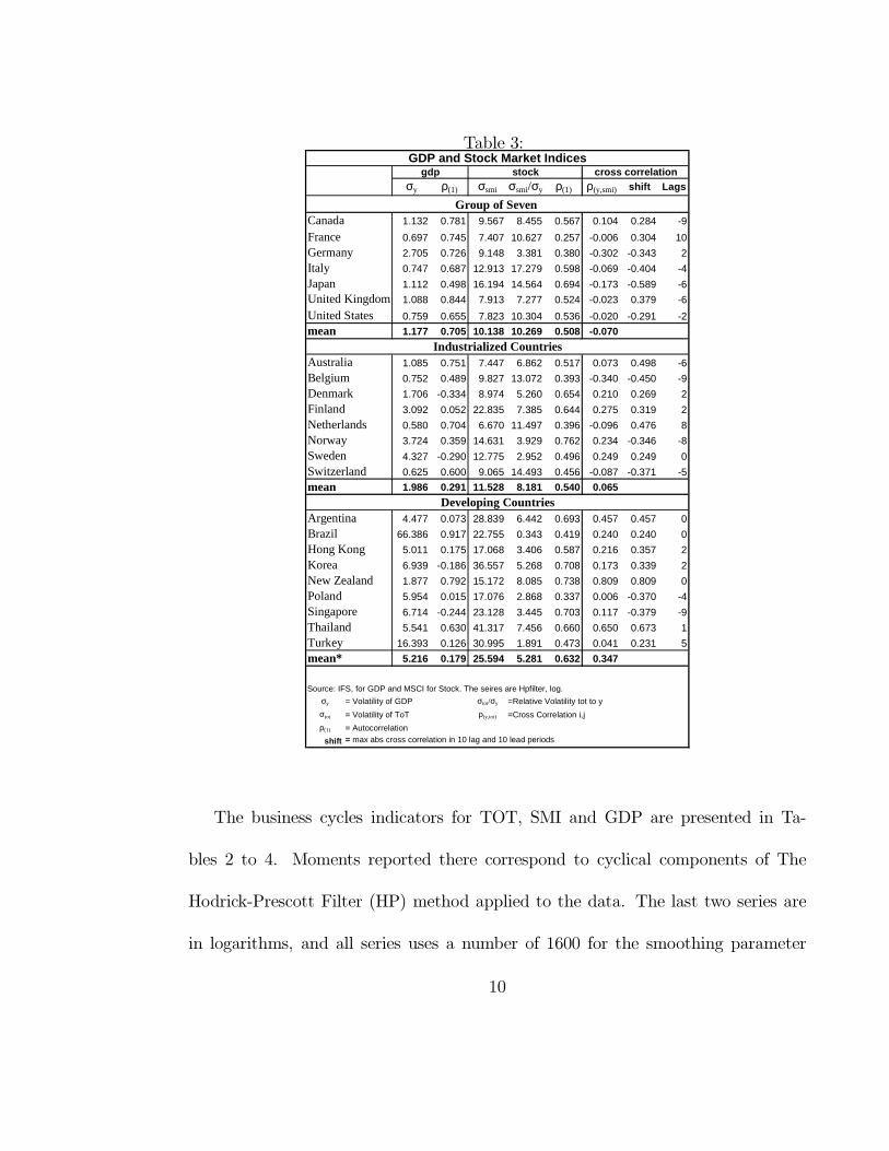
Table 3:σy ρ(1) σsmi σsmi/σy ρ(1) ρ(y,smi) shift Lags

1.132 0.781 9.567 8.455 0.567 0.104 0.284 -9

0.697 0.745 7.407 10.627 0.257 -0.006 0.304 10

2.705 0.726 9.148 3.381 0.380 -0.302 -0.343 2

0.747 0.687 12.913 17.279 0.598 -0.069 -0.404 -4

1.112 0.498 16.194 14.564 0.694 -0.173 -0.589 -6

1.088 0.844 7.913 7.277 0.524 -0.023 0.379 -6

0.759 0.655 7.823 10.304 0.536 -0.020 -0.291 -2

1.177 0.705 10.138 10.269 0.508 -0.070

1.085 0.751 7.447 6.862 0.517 0.073 0.498 -6

0.752 0.489 9.827 13.072 0.393 -0.340 -0.450 -9

1.706 -0.334 8.974 5.260 0.654 0.210 0.269 2

3.092 0.052 22.835 7.385 0.644 0.275 0.319 2

0.580 0.704 6.670 11.497 0.396 -0.096 0.476 8

3.724 0.359 14.631 3.929 0.762 0.234 -0.346 -8

4.327 -0.290 12.775 2.952 0.496 0.249 0.249 0

0.625 0.600 9.065 14.493 0.456 -0.087 -0.371 -5

1.986 0.291 11.528 8.181 0.540 0.065

4.477 0.073 28.839 6.442 0.693 0.457 0.457 0

66.386 0.917 22.755 0.343 0.419 0.240 0.240 0

5.011 0.175 17.068 3.406 0.587 0.216 0.357 2

6.939 -0.186 36.557 5.268 0.708 0.173 0.339 2

1.877 0.792 15.172 8.085 0.738 0.809 0.809 0

5.954 0.015 17.076 2.868 0.337 0.006 -0.370 -4

6.714 -0.244 23.128 3.445 0.703 0.117 -0.379 -9

5.541 0.630 41.317 7.456 0.660 0.650 0.673 1

16.393 0.126 30.995 1.891 0.473 0.041 0.231 5

5.216 0.179 25.594 5.281 0.632 0.347

Source: IFS, for GDP and MSCI for Stock. The seires are Hpfilter, log.

σy = Volatility of GDP σtot/σy =Relative Volatility tot to y

σtot = Volatility of ToT ρ(y,tot) =Cross Correlation i,j

ρ(1) = Autocorrelation

shift = max abs cross correlation in 10 lag and 10 lead periods

United Kingdom

GermanyItaly

Group of Seven

Norway

United Statesmean

AustraliaBelgium

Industrialized Countries

GDP and Stock Market Indices

DenmarkFinlandNetherlands

cross correlation

CanadaFrance

stockgdp

Japan

New ZealandKorea

SwedenSwitzerlandmean

mean*

PolandSingaporeThailandTurkey

Brazil

Developing CountriesArgentina

Hong Kong

The business cycles indicators for TOT, SMI and GDP are presented in Ta-bles 2 to 4. Moments reported there correspond to cyclical components of TheHodrick-Prescott Filter (HP) method applied to the data. The last two series arein logarithms, and all series uses a number of 1600 for the smoothing parameter

10

corresponding to quarterly data. Reports are given for standard deviations in per-centage, first order autocorrelations, contemporaneous correlations, maximum crosscorrelation (shift), and when that happens (Lags), of GDP, TOT and SMI.

The volatility of GDP in Brazil and Turkey are taken off for the calculation ofthe mean when they are compared with the simulations because the devaluation oftheir currency inside the sample period affects the real values of output.

The statistical evidence for the cycles in G7, IC’s, and DC’s presents some facts:1. The shocks to TOT are larger than the volatility of GDP for G7 except for

Germany. The shocks to TOT are smaller than the volatility of GDP for manyDC’s. And there is some mix for IC’s.

2. The persistence of TOT is almost equal across the groups.3. The cross correlation between TOT and GDP is small for almost all countries

and its sign is different across countries.4. The volatility of SMI, is larger in DC’s than the others groups. The volatility

of SMI is also larger than GDP. But the relative volatility between SMI and GDPis larger in G7 than IC’s and from this group to DC’s. That is a direct implicationof the size of volatility of GDP for each country.

5. The cross correlation of SMI with GDP is small for almost all countries buthas different signs: negative in G7 and positive in DC’s.

6. The cross correlation between TOT and SMI does not have a consistent

11

pattern across countries though it exhibits a positive sign for more countries.

Table 4:ρ(tot,smi) shift Lags

0.552 0.552 0 0.191 0.657

0.336 0.336 0 0.221 0.614

0.167 0.232 -1 0.284 0.035

0.275 0.323 -1 0.272 0.554

0.197 0.648 5 0.067 * 0.230

0.124 -0.488 9 0.590 0.758

0.467 0.467 0 0.153 0.328

0.302

0.166 0.586 -3 0.128 0.606

0.610 0.610 0 0.125 0.285

-0.480 -0.480 0 0.791 0.350

0.039 0.414 -4 0.829 0.287

0.116 -0.330 -9 0.356 0.926

0.273 -0.334 8 0.001 * 0.139

0.174 0.412 -4 0.915 0.146

0.030 -0.438 1 0.312 0.670

0.116

0.503 0.613 -1 0.000 * 0.097 *

0.124 -0.279 -6 0.739 0.426

-0.140 0.205 10 0.187 0.001 *

0.489 0.700 2 0.001 * 0.000 *

0.279 0.382 4 0.002 * 0.019 *

-0.574 -0.574 0 0.000 * 0.107

-0.440 -0.504 2 0.246 0.874

0.032 -0.296 -3 0.228 0.000 *

-0.104 -0.117 -7 0.170 0.788

0.021

Source: IFS, for TOT and MSCI for SMI. The series are Hpfilter, SMI is in log.

ρ(tot,smi) = Cross Correlation tot and smi

shift = max abs cross correlation in 10 lag and 10 lead periods

P- Values are for all lags toghether in each variable with 3 lags

GDPt=a1+b1*GDPt-1+...+bn*GDPt-n+c1*TOTt-1+...+cn*TOTt-n+

D1*Stockt-1+...+dn*Stockt-n+errort,

Germany

cross correlationSMI and TOT

CanadaFrance

United KingdomUnited Statesmean

ItalyJapan

mean

Hong KongKoreaNew ZealandPoland

P-Values

SingaporeThailandTurkey

mean

ArgentinaBrazil

NetherlandsNorwaySweden

Developing Countries

stocktot

Group of Seven

Industrialized Countries

Switzerland

AustraliaBelgiumDenmarkFinland

In Table 4, there is also a test with the p-value of the Wald test to check if thelags of TOT or SMI affect current GDP, on a VAR model with these three series.

12

P-values are for three lags together for each variable, TOT and SMI, are significallydifferent from zero,

GDP = a+ b ∗GDP+ ...+ b ∗GDP + c ∗ TOT+ ...

+c ∗ TOT + d ∗ SMI+ ... + d ∗ SMI + ε

The result shows that for many developing countries the terms of trade and stockmarket indices shocks explain part of the GDP volatility, but it does not happen forG7 and industrial countries.

3 Model

In this economy, there is a representative agent who lives forever. The preferencesare given by maximizing the present value of expected utility given by a compositegood, C, leisure time, L, and subjective exogenous discount factor, β.

maxU (C) = E

[ ∑

β(C (L))

1− γ]

(1)

L = 1− l − l − l

where E is the expectations operator, conditional on information available attime t. In each period of the utility function, leisure time enters in unitary - elasticityform where ω governs labor supply elasticity. Leisure time is equal to total time

13

minus the time spend in each production sectors; constant in both tradeable sector:exportable, l, and importable, l , and variable in nontradeable sector, l .

The composite good has the following function:

C = [(C ) + n ] (2)

C = x f (3)

γ > 1 , µ > −1, 0 > β,α > 1, ω > 0

Tradeable, C , and nontradeable, n, goods are represented in constant-elasticityof substitution (CES) form and

is its elasticity of substitution. Tradeable areexpressed in Cobb-Douglas unitary-elasticity form with α is the share of exportablegoods, x, and (1− α) is the share in importable goods, f. The intertemporalelastiticy of substitution in aggregate consumption is

.The output is given by the aggregate production function for each sector, exports,

(Y ), imports,(

Y )

, and non-traded, (Y ):

Y = ε A (K ) (l ) (4)

Y = εA (K

)

(l) (5)

Y = εA(K

) (l ) (6)

K = K +K (7)

Production for each sector follows a Cobb-Douglas technology, but with differ-ences in the shares for capital; the tradeable sector has a constant labor supply.

14

Nontradeable sector has constant capital and variable labor supply. K , K and

K are capital stocks; since trade sector capital is homogenous, the capital for eachperiod is the sum of the capital in both sectors. A , A and A are total factor pro-ductivity effects. ε , ε and ε are random shocks for each function of production.

εP x + f + I + ψ = εP Y + Y (8)

P n = P Y (9)

K = (1− δ)K + I (10)

Equation (8) and (9) are the household budget constraint. All the prices areexpressed in term of importables (as numeraire), so P is world relative price ofexportables and P is the endogenous domestic relative price of nontradeables. ε

is an exogenous shock to exportable goods and also the shock to the terms of trade.The equation (10) is the change of capital stock between dates t and t + 1 that

evolves with net investment, I.Capital has a depreciation rate, δ. The household-firm pays a deadweight instal-

lation cost of capital following a quadratic adjustment cost function,

ψ = χ2K (I)

"OR" (11)

or ψ = χ2 (I) "M" (12)

Two different functions are considered: The first uses Obstfeld and Roggoff(1996), "OR". The second uses Mendoza (1995), "M". Using "OR" presents the

15

advantage that the marginal and average Tobin’s q are equal. However the value ofadjustment costs are relatively small.

This specific cost function shows an increasing marginal cost of investment; andcaptures the observation that a faster pace of change requires a greater than propor-tional rise in installation costs. The representative agent-firm pays this cost. Withthat, it is possible to distinguish a net investment value, I, and a gross investmentthat is the sum of net investment and the cost function, I + ψ.

ε = exp (υ)

υ = (1− ρ) υ + ρυ+ ϑ i = p, x, f, n

ϑ iid N (0,Σ) ,

The random shocks ε , ε , ε and ε are assumed to follow first order MarkovProcesses. The random variable υ

follows an autoregressive process AR(1).For simplicity the model presented here does not incorporate international assets

and thus does not have capital mobility. The openness of financial markets with anew international asset which the household can borrow or lend at the internationalfixed interest rate requires a new endogenous variable to solve the problem of steadystate. One approach uses an endogenous discount factor function, as Mendoza(1991), Smith-Grohé and Uribe (2001), or Epstein and Zin (1989). Those functionsimply at least another Euler equation, and they use many more parameters for the

16

parameterized expectation algorithms.

3.1 Equilibrium and Dynamic Programming Formulations

The competitive equilibrium is defined by stochastic processes I, K, x, f,n, l , p , K

, K , where the household optimizes the expected value of

utility subject to the budget constraint in the tradeable sector, the market clears innon-traded sector, and the two restrictions on capital, equations (7) and (10), aresatisfied.

The Lagrangian for solving the model is:

E

[ ∑

β

(

11− γ

(

(xf

) + n)

(1− l − l − l)

+φ(

εA(K

) (l ) − n

)

+

θ (K −K −K

)− q (K− (1− δ)K − I)+

λ ( εP εA (K

) (l) − I − εP x

+εA (K )

(l) − f − χ2K (I)

)) ]

The variable λ is the familiar Lagrangian multiplier representing the marginalutility of wealth. The term q, known as Tobin’s q, represents the Lagrange multiplierfor the evolution of capital - it is the "shadow price" for new capital.

Maximizing the Lagrangian with respect to I, K, x, f, n, l , K , K , q,

17

θ, λ, φ, yields the following first order conditions (Using "OR"):

I : q = λ(χIK

+ 1)

(13)

K : q = βE

[

θ+ (1− δ) q+ χ2( IK

)

λ

]

(14)

x :(

((x) (f)) + n) (1− l − l − l )

((x) (f)) αx = λεP (15)

f :(

((x) (f)) + n) (1− l − l − l )

((x) (f)) (1− α)f = λ (16)

l :(

((x) (f)) + n)

(1− l − l − l )ω = φαεA(K

) (l ) (17)

n :(

(x f

) + n) (1− l − l − l )n = φ (18)

K : θ = λ (1− α ) εε P

A (K ) (l ) (19)

K : θ = λ (1− α) εA (K

)

(l) (20)

λ : εP x + f + I + χ

2K(I) = εP

Y + Y

(21)

φ : n = εP A(K

) (l ) (22)

θ : K = K +K

(23)

q : K = (1− δ)K + I (24)

The market clearing conditions are as follow: first, the Current Account is inequilibrium and equal to zero for each period. By definition it gives a restriction

18

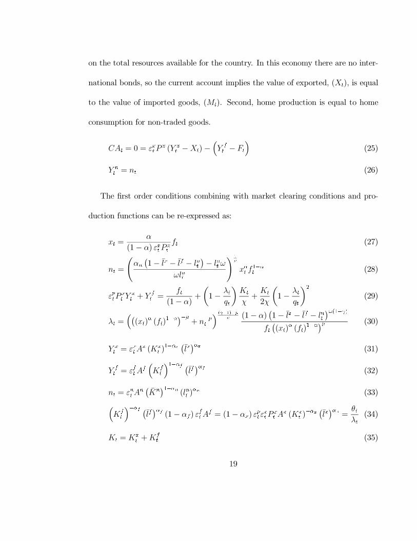
on the total resources available for the country. In this economy there are no inter-national bonds, so the current account implies the value of exported, (X), is equalto the value of imported goods, (M). Second, home production is equal to homeconsumption for non-traded goods.

CA = 0 = εP (Y −X)−

(

Y − F

)

(25)

Y = n (26)

The first order conditions combining with market clearing conditions and pro-duction functions can be re-expressed as:

x = α(1− α) εP

f (27)

n =(α

(1− l − l − l )− l ωωl

) x f (28)

εP Y

+ Y = f

(1− α) +(

1− λq) Kχ + K

2χ(

1− λq)

(29)

λ =(

((x) (f)) + n) (1− α) (1− l − l − l )

f ((x) (f)) (30)

Y = εA (K ) (l) (31)

Y = εA (K

)

(l) (32)

n = εA(K

)

(l ) (33)(

K ) (l) (1− α) εA = (1− α) ε

!εP A (K ) (l) = θλ (34)

K = K +K (35)

19

K =(

(1− δ) + 1χ( qλ − 1

))

K (36)

p = φλ =

n f((x) (f))

(1− α) (37)

q =(

1 + χ IK

)

λ (38)

q = βE[

θ+ (1− δ) q+ χ2( IK

)

λ]

(39)

Equation (38) states that the shadow price of capital equals the marginal cost ofinvestment, including installation costs. The condition can be rewritten as a versionof the investment equation posited by Tobin (1969), with the only difference thattraditional Tobin’s q is that here q is a "nominal" variable, because it is multipliedby marginal value of wealth of the representative agent.

The last equation is the only Euler equation in this model; this condition is aninvestment Euler equation. The above equation also shows that the solution for qcomes from forward-looking stochastic process. It states that at, an optimum for thehousehold-firm, the date t shadow price of an extra unit of capital is the discountedsum of:

1. The capital’s marginal product next period.2. The shadow price of capital on the next date, t + 1, net of depreciation.3. The capital’s marginal contribution to lower installation costs next period.The price of non-traded goods adjusts instantaneously to clear the market for

non-traded goods.

20

Thus the model has only one "forward-looking" stochastic Euler equation, whichdetermine q. This variable, together with rest of the equations gives the solutionfor each period with a initial capital for each period and a particular realization ofthe shocks.

4 Solution Algorithm

Several algorithms are used to solve a model like this.Mendoza (1995) uses value function iteration and transition probability itera-

tions using discrete grids to approximate the state space. This method is memoryintensive and uses a limited number of state variables and few shocks. For thisreason this paper uses two other algorithms: first, Linear Quadratic approximation(LQ) and second, the Parameterized Expectation Algorithm (PEA).

The LQ method uses a second order approximation to the steady state. Itis necessary to combine the FOC’s to reduce the number of equations to equal thenumber of state variables and the restrictions are limited to linear equations. Linearquadratic methods are widely used in RBC models. The optimal linear decisionrule is the same for the deterministic and stochastic versions this is the well-knowncertainty equivalence property of this algorithm. This gives a good approximationwhen the shocks are small and the model stays close to its steady state.

21

The PEA uses a parametric function of the state variables to approximate eachexpectation term in the Euler equations. This method adjusts these function tominimize the error between the expected value and the ex-post value of this expec-tation. The advantage of this algorithm is that it permits a richer model with morevariables, shocks and no linearity. The limitations are that it is time consuming, incomputational terms.

The PEA approximates the forward-looking expectation as non-linear functionalforms of the information available at each period. The polynomial approach workswell when the model has few parameters and there are few constraints as in Maliarand Maliar (2003). However it is difficult to find the solution when there are manyconstraints as in this model. For this reason, this study uses a neural networkapproach, where variables and parameters enter as non linear functions. For thisreason the algorithm uses a global search, for the optimization problem.

The rest of this section works with both methods LQ and PEA to solve themodel.

4.1 Linear Quadratic Approximation

This subsection summarizes the features for solving the model with linear quadraticapproximation, following to McGrattan (1994), Urrutia (1998) and Pacharoni (2000).The optimization problem is simplified by expressing it as a dynamic programming

22

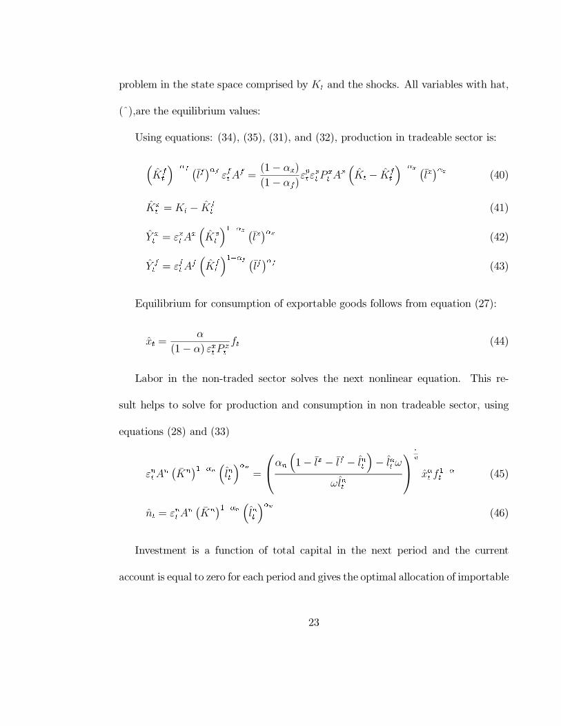
problem in the state space comprised by K and the shocks. All variables with hat,(ˆ),are the equilibrium values:

Using equations: (34), (35), (31), and (32), production in tradeable sector is:(

K

)(l) εA = (1− α)

(1− α)εεP

A(

K − K

)(l) (40)

K = K − K

(41)

Y = εA

(

K

)(l) (42)

Y = ε A (K

)

(l) (43)

Equilibrium for consumption of exportable goods follows from equation (27):

x = α(1− α) ε P

f (44)

Labor in the non-traded sector solves the next nonlinear equation. This re-sult helps to solve for production and consumption in non tradeable sector, usingequations (28) and (33)

ε A(K

) (l ) =

α

(

1− l − l − l )

− l ωωl

x f (45)

n = ε A(K

) (l ) (46)

Investment is a function of total capital in the next period and the currentaccount is equal to zero for each period and gives the optimal allocation of importable

23

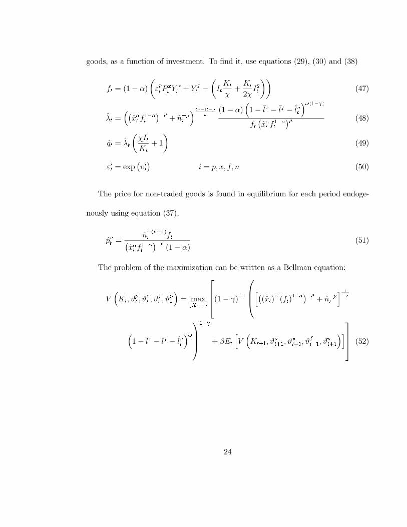
goods, as a function of investment. To find it, use equations (29), (30) and (38)

f = (1− α)(

ε P Y + Y −

(

I K

χ + K

2χI ))

(47)

λ =(

(x f ) + n

)

(1− α)(

1− l − l − l)

f (x f ) (48)

q = λ(χIK + 1

)

(49)

ε = exp (υ) i = p, x, f, n (50)

The price for non-traded goods is found in equilibrium for each period endoge-nously using equation (37),

p = n f

(x f ) (1− α) (51)

The problem of the maximization can be written as a Bellman equation:

V(

K, ϑ , ϑ , ϑ , ϑ

)

= max

(1− γ)

[

((x )! (f )!)

" + n

" ]

#$

(

1− l% − l& − l' )(

)

+ βE [

V(

K *, ϑ+ *, ϑ% *, ϑ&

*, ϑ' *)]

(52)

24

The laws of motion of capital and the law of shocks are given by:

K * = (1− δ)K + I

υ = (1− ρ) υ + ρυ

+ ϑ i = p, x, f, n

ϑ iid N (0,Σ) ,

where the shocks are iid normal with a variance and covariance matrix Σ.With a second order Taylor expansion around the steady state the problem is

reduced to

V (x) = max[xQx+ 2yWx+ yRy + βV (x)] (53)

subject to :

x = Ax+By + ε (54)

Following Urrutia (1998), to solve this Bellman equation it is useful to considera guess of this expectation and to check if this guess is the solution:

V (x) = xPx+ d

where d = β(1− β)trace(PΣ)

After, it is necessary to compute the optimal decision rule through the partialderivative. With this, the decision rule is y = Gx, where

G = − (Q+ βBPB)(W + βBPA)

25

This optimal decision rule has two properties: First, it is a linear function of thestate variables. Second, G is independent of the stochastic structure of the problem,and in particular of the variance — covariance of the shocks, Σ. Both properties arespecific to linear quadratic models.

To check if the guess is a valid solution, one verifies that it solves the followingequation.

P = R+ βAPA− (W + βAPB) (Q+ βBPB)(W + βBPA)

The last equation is known as Ricatti’s equation. The matrix P is solved byiteration.

The next step in this methodology is to find the steady state of the model.Define the next auxiliary equations:

D =( α(1− α)P

)

E = (1 + χδ)( 1β − 1 + δ

2)

+ δ2

H =(α

(1− l − l − l)− lωωl

)

Z = D ((1 +H)) (1− l − l − l) (1− α)

With them and equations (25) to (38) and assuming the variables are determin-istic and stable for all periods, the steady state values are given by the following

26

equations

K =(A (1− α)

E)

K =(AP (1− α

)E

)

K = K +K

I = δK

Y = A (K ) (l)

Y = A (K) (l)

f = (1− α)(

P Y + Y − I − χ2KI

)

λ = f Z

q = λ (1 + χδ)

θ = Eλ

x = α(1− α)P

f

n = Y = HDf

K = A(K

) (l)

To find labor in the non-tradeable sector in steady state, l, I use the value ofthe calibration and find the value of constant capital in this sector.

The vector and matrices implied by this method for this study are (where thecapital U are the partial derivative of utility function at steady state value with

27

respect variable i and j :

x =

Kϑ

ϑ

ϑ

ϑ1

; Q =

U U U U U U

U U U U U U

U U U U U U

U U U U U U

U U U U U U

U U U U U 2U

y =

IL

; W =

U U U U U 2U

U U U U U 2U

R =

U U

U U

B =

1 00 00 00 00 00 0

; A =

1− δ 0 0 0 0 00 ρ 0 0 0 1− ρ0 0 ρ 0 0 1− ρ0 0 0 ρ 0 1− ρ

0 0 0 0 ρ

1− ρ

0 0 0 0 0 1

28

ϑ =

0ϑϑϑ

ϑ

0

; Σ =

0 0 0 0 0 00 σ σ σ σ 00 σ σ σ σ 00 σ σ σ σ 00 σ σ σ σ 00 0 0 0 0 0

This method does not impose any discretization or grid for the space state vari-ables. This is a good approximation only when the model is around the steadystate. This method is inappropriate when the initial conditions are far away fromthe steady state or for economies where the shocks have a large variance. Someresearches find this method sufficient for almost any RBC Model. However in thisstudy this method fails to generate volatility, as it is observed in the data.

4.2 Parameterized Expectations Algorithm

This subsection studies the parameterized expectations approach to this model.Following Marcet (1988, 1993), Den Haan and Marcet (1990, 1994), and Duffy andMcNelis (2001), the approach of this study is to "parameterize" the forward-lookingexpectation in this model, with non-linear functional forms on the Euler equation

29

(39),

q = βE[

θ+ (1− δ) q+ χ2( IK

)

λ]

(55)

Combining this equation with (38) and (30) finds the time used in labor in the non-traded sector production as a function of some expectation function and that is thevariable that is parameterized.

λ =(

((x) (f)) + n

) (1− α) (1− l − l − l )

f ((x) (f))

I =( qλ − 1

) Kχ

l = E

1− l − l−

βf (x f ) [θ+ (1− δ) q+ (

)λ

]

(

+ 1

)

(1− α)(

(x f ) + n

)

(56)l ψ (z; Ω)

z = K/K, ε! , ε" , ε# , ε$

The term ψ % is the expectation approximation function. The symbol z repre-

sents a vector of observable "instrument" variables known at time t: in fact, I usethe state variables: the initial capital at t which is predetermined at that moment,

30

and the realization of the different shocks at t. The term K is the value of capitalin steady state. The symbol Ω represents the parameters for the approximationfunction ψ %

.Judd (1996) classifies this approach as a "projection" or a "weighted residual"

method for solving functional equations, and notes that the approach was originallydeveloped by Williams and Wright (1982, 1984, 1991). These authors pointed outthat the conditional expectation of the future grain price is a "smooth function" ofthe current state of the market, and that this conditional expectation can be usedto characterize equilibrium.

Parameterizing equation (56) rather than equation (55) has at least three advan-tages. First, it prevents small errors in the approximation of q from being amplifiedin the variation of I. Second, Parameterizing equation (56) the remaining equa-tions have closed form solutions. Third, from the FOC’s there is a condition betweenparameters and labor in non-traded sector that must be satisfied in each period:

l$ < α$(1− l" − l#)α$ + ω

and putting the right side of the last equation as the maximun value of theparameterized expectation on labor in non tradeable goods, gives no violation ofthe condition for each period. The combination of these three advantages givesmore accurate and faster solutions.

31

The functional form for ψ % is usually a second-order polynomial: see, for example,

Den Haan and Marcet (1994), Schmitt-Grohé and Uribe (2002). However, Duffyand McNelis (2001) have shown that neural networks have produced results withgreater accuracy for the same number of parameters, or equal accuracy with fewerparameters, than the second-order polynomial approximation.

The model was simulated until convergence was obtained for the expectationalerrors. In the algorithm, the following non-negativity constraints for consumptionand the stocks of capital for next period were imposed:

C" > 0 (57)

K ≥ 0 (58)

The latter was achieved by restricting capital for next period to be bigger thanzero, which implies that is there is some degree of reversibility on the investment.

5 Parameters

The section discusses the calibration of parameters, initial conditions, and stochasticprocesses for the exogenous variables of the model.

The selections of the parameters are from other studies. The there three setof the parameters: First, Argentina (ARG), follows Pacharoni (2000). Second andthird, developing countries (DC’s), and industrialized countries (G7), follow Men-

32

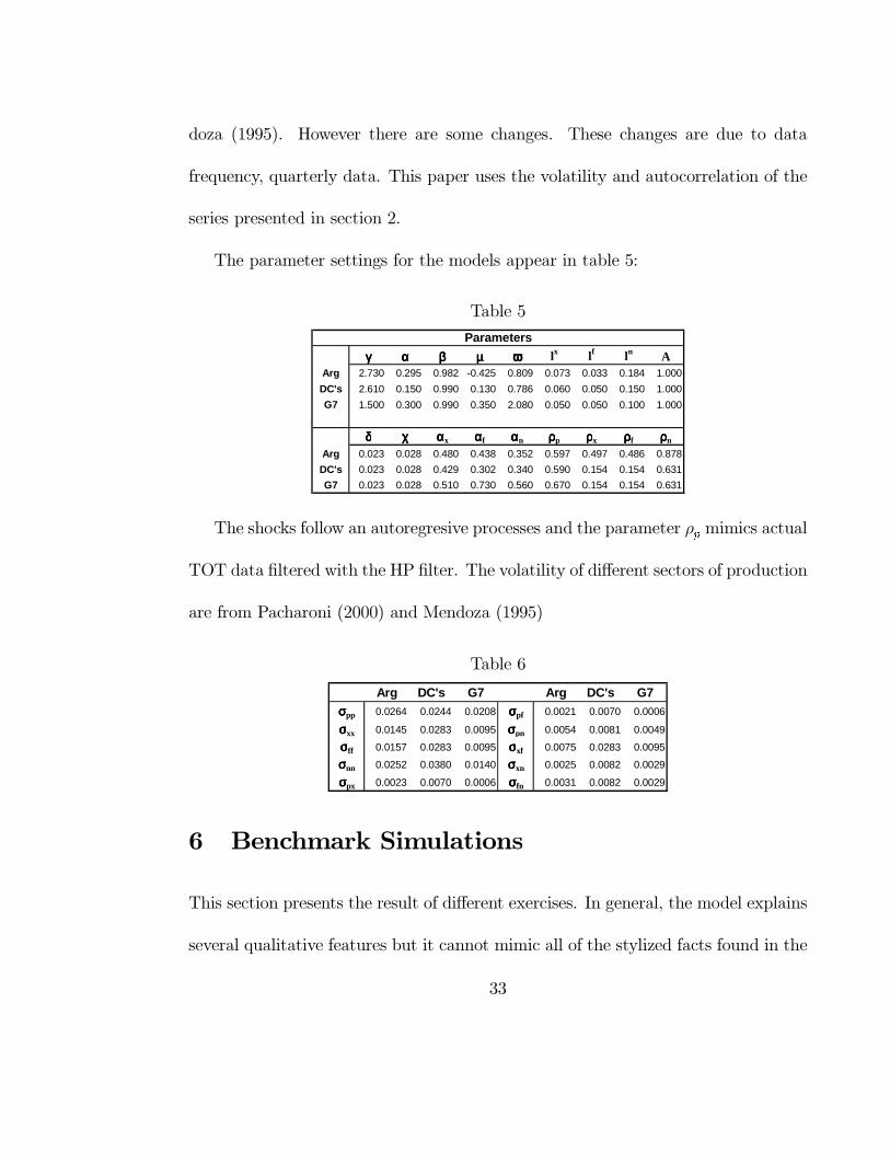
doza (1995). However there are some changes. These changes are due to datafrequency, quarterly data. This paper uses the volatility and autocorrelation of theseries presented in section 2.

The parameter settings for the models appear in table 5:

Table 5γγγγ αααα ββββ µµµµ ωωωω lx lf ln A

Arg 2.730 0.295 0.982 -0.425 0.809 0.073 0.033 0.184 1.000

DC's 2.610 0.150 0.990 0.130 0.786 0.060 0.050 0.150 1.000

G7 1.500 0.300 0.990 0.350 2.080 0.050 0.050 0.100 1.000

δδδδ χχχχ ααααx ααααf ααααn ρρρρp ρρρρx ρρρρf ρρρρn

Arg 0.023 0.028 0.480 0.438 0.352 0.597 0.497 0.486 0.878

DC's 0.023 0.028 0.429 0.302 0.340 0.590 0.154 0.154 0.631

G7 0.023 0.028 0.510 0.730 0.560 0.670 0.154 0.154 0.631

Parameters

The shocks follow an autoregresive processes and the parameter ρ mimics actualTOT data filtered with the HP filter. The volatility of different sectors of productionare from Pacharoni (2000) and Mendoza (1995)

Table 6 Arg DC's G7 Arg DC's G7

σσσσpp 0.0264 0.0244 0.0208 σσσσpf 0.0021 0.0070 0.0006

σσσσxx 0.0145 0.0283 0.0095 σσσσpn 0.0054 0.0081 0.0049

σσσσff 0.0157 0.0283 0.0095 σσσσxf 0.0075 0.0283 0.0095

σσσσnn 0.0252 0.0380 0.0140 σσσσxn 0.0025 0.0082 0.0029

σσσσpx 0.0023 0.0070 0.0006 σσσσfn 0.0031 0.0082 0.0029

6 Benchmark Simulations

This section presents the result of different exercises. In general, the model explainsseveral qualitative features but it cannot mimic all of the stylized facts found in the

33

data.

Table 7 Table 8

OR M OR My 1.177 2.330 1.990 2.116 2.108

(0.192) (0.163) (0.119) (0.118)

qt 10.138 0.698 0.351 2.841 2.833(0.097) (0.069) (0.169) (0.168)

c 0.386 0.997 2.078 2.072(0.057) (0.1) (0.126) (0.126)

I 7.390 7.316 5.748 5.814(0.627) (0.62) (0.295) (0.284)

n 0.300 0.299 0.065 0.062(0.03) (0.03) (0.004) (0.004)

k 0.349 0.346 0.282 0.284(0.073) (0.072) (0.03) (0.029)

qt 8.613 0.300 0.176 1.344 1.345c 0.166 0.501 0.983 0.984i 3.172 3.676 2.722 2.765n 0.129 0.150 0.031 0.030k 0.150 0.174 0.134 0.135

relative to y

Volatility - G7LQ PEA

DataOR M OR M

y 5.216 4.050 3.552 2.757 2.853(0.337) (0.298) (0.127) (0.133)

qt 25.878 0.559 0.501 12.052 12.133(0.098) (0.079) (0.708) (0.745)

c 1.333 3.009 4.986 4.994(0.141) (0.296) (0.293) (0.312)

i 8.936 7.887 5.831 5.989(0.764) (0.663) (0.274) (0.286)

n 0.318 0.306 0.087 0.086(0.032) (0.032) (0.003) (0.004)

k 0.323 0.288 0.259 0.265(0.053) (0.047) (0.025) (0.025)

qt 4.961 0.138 0.141 4.373 4.255c 0.329 0.847 1.809 1.751I 2.206 2.220 2.119 2.103n 0.079 0.086 0.032 0.030k 0.080 0.081 0.094 0.093

relative to y

Volatility - DC'sLQ PEA

data

Table 9 Table 10

OR M OR My 4.476 2.115 2.228 2.0882 2.120

(0.203) (0.242) (0.133) (0.137)

qt 28.839 1.192 0.886 8.9625 9.136(0.145) (0.149) (0.655) (0.654)

c 2.411 2.020 3.571 3.569(0.346) (0.278) (0.253) (0.252)

i 7.158 6.924 4.7615 5.034(0.735) (0.708) (0.3) (0.315)

n 0.825 0.809 0.1785 0.156(0.113) (0.111) (0.008) (0.008)

k 0.404 0.392 0.3034 0.324(0.095) (0.093) (0.039) (0.038)

relative to yqt 6.443 0.564 0.398 4.293 4.311c 1.140 0.907 1.710 1.684i 3.384 3.108 2.286 2.381n 0.390 0.363 0.086 0.074k 0.191 0.176 0.145 0.153

LQ PEAVolatility - Argentina

data

OR M OR M

y 0.705 0.510 0.500 0.554 0.552qt 0.508 0.930 0.773 0.470 0.567c 0.621 0.818 0.846 0.849i 0.470 0.471 0.686 0.691n 0.954 0.954 0.300 0.317k 0.596 0.596 0.666 0.670

tot 0.656 0.610 0.610 0.558 0.558

qt -0.070 -0.465 0.369 0.544 0.562c 0.717 -0.218 0.023 0.016i 0.989 0.986 0.827 0.825n 0.165 0.185 0.549 0.536k -0.648 -0.638 -0.784 -0.775

tot -0.165 0.868 0.844 0.878 0.879

qt 0.302 -0.334 0.522 0.510 0.552c 0.607 -0.316 -0.071 -0.074i 0.856 0.856 0.683 0.682n 0.044 0.043 0.548 0.539k -0.635 -0.639 -0.612 -0.603

Crosscorrelation with TOT

Correlations - G7LQ PEA

Crosscorrelation with Y

data

First Order Autocorrelation

34

Table 11 Table 12

OR M OR M

y 0.255 0.160 0.157 0.238 0.193qt 0.591 0.841 0.718 0.529 0.279c 0.573 0.613 0.522 0.817i 0.199 0.193 0.193 0.578n 0.927 0.927 0.184 0.393k 0.606 0.593 0.829 0.593

tot 0.443 0.543 0.543 0.432 0.491

qt 0.301 -0.342 -0.390 -0.699 0.088c 0.517 -0.306 0.702 0.146i 0.982 0.985 0.249 0.698n -0.015 -0.034 0.333 0.157k -0.315 -0.409 0.084 -0.609

tot 0.040 0.532 0.544 0.446 0.470

qt 0.019 -0.254 -0.611 -0.275 -0.129c 0.588 -0.312 0.306 0.144i 0.570 0.562 0.127 0.422n 0.013 0.002 0.052 -0.044k -0.532 -0.554 0.033 -0.357

Crosscorrelation with TOT

Correlation - DC'sLQ PEA

Crosscorrelation with Y

data

First Order AutocorrelationOR M OR M

y 0.073 0.531 0.525 0.611 0.620qt 0.693 0.898 0.784 0.229 0.268c 0.809 0.811 0.857 0.867i 0.645 0.644 0.681 0.694n 0.961 0.961 0.543 0.571k 0.798 0.796 0.684 0.695

tot 0.604 0.544 0.544 0.495 0.495

qt 0.457 -0.476 -0.567 -0.461 -0.472c 0.412 -0.190 0.407 0.392i 0.802 0.806 0.915 0.918n 0.255 0.199 -0.391 -0.413k 0.347 0.381 -0.881 -0.879

tot 0.356 0.511 0.619 0.648 0.647

qt 0.503 -0.177 -0.548 -0.330 -0.350c 0.349 -0.106 0.288 0.276i 0.496 0.496 0.569 0.567n -0.075 -0.076 -0.189 -0.198k 0.394 0.399 -0.453 -0.447

Crosscorrelation with TOT

Correlations - ArgentinaLQ PEA

Crosscorrelation with Y

data

First Order Autocorrelation

Tables 7 to 12 compare business cycles in the models with those observed inthe seven largest industrialized countries, G7, developing economies, DC’s, and Ar-gentina, ARG.

Tables 7 to 9 presents the volatility of key variables: product, y, Tobin’s q,qt, consumption, c, investment, i, labor, n, and capital, k. They also show therelative volatility for each variable to the GDP, y. Tables 10 to 12 present the firstorder autocorrelation of the same variables plus the Terms of Trade, tot, and theircross-correlation with the GDP and Tobin’s q.

Vertically the tables are divided in three sections: data, Linear Quadratic, LQ,and Parametrized Expectation Algorithm, PEA. The column called "data" presents

35

the values of actual data from tables 2 to 4. LQ has two models, with differentadjustment cost functions for capital, one following Obstfeld and Roggoff (1996),"OR", and the other following Mendoza (1995), "M"; the exercise was realizedon 100 simulations and 76 observations. PEA also has two models with the sameadjustment cost functions. Simulations for PEA models has 500 simulations and300 observations.

The goal of this study is to understand the implication of the volatility in thestock markets through Tobin’s q, for developing countries. The benchmark simula-tions for developing countries underestimate these values but their relative volatilityis close to the value found in the data using PEA, but do not match well with LQ.

For the G7 countries the simulation does not replicate the volatility for GDP. Itis almost twice as in the actual data. For the volatility of qt, the simulations predictvalues greater than the GDP using PEA though far away from the value in thedata.

In the DC’s, the volatility of production is underestimated by half the value ofPEA estimate, and something similar with LQ. But the Tobin’s q has a good fit withthe data for a relative volatility for PEA, given that the model underestimates also ahalf of the data business cycles. The consumption has the same problem as the G7.The volatility is larger than y by 1.7 times. The volatility predicted by the modelsfor investment is twice than their productions, but this value is close to Mendoza

36

(1995). The volatility of the labor in the non-traded sector is underestimated in themodel, all versions of the model give volatility less than 10 percent.

For Argentina, the volatility of GDP the model predicts is a little less than ahalf of the data, and almost one third of the stock market indices. The volatility inTobin’s q relative to GDP is more than two thirds that of the data.

The autocorrelations for TOT are close to the data by construction. They aregenerated to mimic the data, when the calibration was made.

In the G7 versions, the autocorrelations of GDP are around 0.7 of the data. Theautocorrelations of Tobin’s q are close to the data for PEA and LQ overestimatesthem. For DC’s the values of autocorrelations of GDP and Tobin’s q are close to thedata for the version of the model of OR using PEA algorithm, the other versionsunderestimate GDP. For Argentina, the data have no autocorrelation for GDP andthe model gives a number around 0.5; the Tobin’s q is overestimated with LQ andunderestimated with the PEA.

The cross correlation between Tobin’s q and the production for the three sectorsdoes not fit with the data; for DC’s and for Argentina it has the different sign. Crosscorrelation of the terms of trade and product are over estimated for all the models,but they are so far away of the data for G7 (and, with different sign) and DC’s. ForArgentina the models overestimate them twice.

37

The cross correlation between Tobin’s q and terms of trade is over estimated bya factor of 1.6 in G7 models. DC economies do not present cross correlations in thestock markets indices while the models predict a negative one.

7 Sensitivity Analysis

This section examines the role that some parameters play in explaining the proper-ties of business cycles in the model.

Table 13 Table 14

PEA-OR 19 19 22χ=0 χ=0.028 χ=0.028

y 1.957 1.961 1.949qt 2.854 2.838 2.849c 2.110 2.099 2.104i 5.221 5.136 5.451n 0.072 0.074 0.065k 0.232 0.227 0.234

y 1.000 1.000 1.000qt 1.459 1.447 1.462c 1.078 1.071 1.080i 2.669 2.620 2.796n 0.037 0.038 0.033k 0.119 0.116 0.120

Volatility - G7

relative to y

Parameters in Expectations

A=0.3 A=1.0OR OR

y 2.831 2.757(0.13) (0.127)

qt 11.981 12.052(0.692) (0.708)

c 4.945 4.986(0.291) (0.293)

i 5.902 5.831(0.263) (0.274)

n 0.083 0.087(0.003) (0.003)

k 0.260 0.259(0.025) (0.025)

qt 4.234 4.373c 1.747 1.809i 2.088 2.119n 0.030 0.032k 0.092 0.094

relative to y

Volatility - DC's

PEA

Table 13 examines changes in the number of parameters of the function ψ

, forPEA for the industrial countries. There is no theory to use one or another specificfunction as the parameterized function. This paper does not find any change whenit uses a constant term in the last hidden layer of the neural network, the change

38

between 19 and 22 parameters. There are no changes in the volatility of the timeseries when the numbers of neurons are the same, and estimates are not significantlyaffected by the functional form used in the nerual net.

This study pins down the two versions of the adjustment cost used in this paper.In each table there are the results for both functions. The changes in the volatilityare small using one or the other. Table 13 is also a comparison of the parameterthat governs the adjustment cost function, χ, when it is equal to zero or as usual inthe literature 0.028.

Another analysis is study the scale of production, A. It is usually fixed at 1, butas Mendoza (1995) presents a value of 0.3 for developing economies, it is due thecomparison with developed countries. Developing countries are richer than devel-oped ones if the parameter A is the same. Table 14 examines the volatility of keyvariables in developing economies where their values are the same. The model doesnot find difference in the volatility.

39

Table 15 Table 16

(1) TOT (2) TOT (3) TOTy 2.330 1.397 2.803 0.3167 2.089 0.731qt 0.698 0.641 11.966 0.3976 8.978 0.837c 0.386 0.636 4.876 0.391 3.517 0.806I 7.390 4.567 5.895 0.174 4.942 0.457n 0.300 0.031 0.064 0.0024 0.107 0.013k 0.349 0.183 0.270 0.007 0.334 0.019

y 1.000 1.000 1.000 1.000 1.000 1.000qt 0.300 0.459 4.272 1.256 4.360 1.145c 0.166 0.455 1.740 1.235 1.798 1.102i 3.172 3.270 2.108 0.550 2.286 0.625n 0.129 0.022 0.023 0.008 0.113 0.017k 0.150 0.131 0.097 0.022 0.117 0.026

(1)-(3) from Tables 7-9

relative to y

Volatility - only shock TOTG7 DC's ARG

γγγγ= 2.61 γγγγ= 60y 5.216 4.050 4.036

(0.337) (0.337)

qt 25.878 0.559 11.830(0.098) (2.41)

c 1.333 3.331(0.141) (0.347)

i 8.936 10.300(0.764) (0.914)

n 0.318 0.426(0.032) (0.043)

k 0.323 0.400(0.053) (0.069)

y 1.000 1.000 1.000qt 4.961 0.138 2.932c 0.329 0.825i 2.206 2.552n 0.079 0.106k 0.080 0.099

relative to y

Volatility - DC'sLQ - OR

data

Table 15 examines the volatility of the model produced only by a shock in theterms of trade. The result shows small volatility in Tobin’s q. It predicts morevolatility in Tobin’s q than in GDP for developing economies and less for industrialcountries.

Table 16 presents a change in the parameter of risk aversion from 2.61 to 60, forLQ approximation, the model explains almost half of the volatility of the Tobin’s q.

8 Conclusion

This paper conducts a quantitative examination of the link between terms of tradeshocks and business cycles by comparing numerical solutions of the competitiveequilibrium of a dynamic stochastic model of a small open economy with actual

40

business cycles, especially to understand the implication of the volatility in thestock markets through the Tobin’s q, for developing countries. In the model, acombination of consumption in exportable, importable and non-traded goods andleisure time give the welfare of the household. The firms, owned by the household,produce three different goods, using capital and labor: exportable, importable andnon tradeable. World markets of good are competitive. The rest of the world hasinelastic demand and supply at international prices for traded goods.

The result, that the model solved by parameterized expectations approach withglobal search for developing countries, shows that relative volatility of the Tobin’sq to the output replicates that found in the data between Stock Market Indices andGDP during the last decade.

The comparison between the control case as the G7 and developing economiesgives some implications for the different behavior of the volatility of the Tobin’s q;and the case of Argentina gives one "country" example of that result.

The paper has made some comparison and sensitivity analysis: one is betweendifferent adjustment cost function. Using a marginal capital cost as Obstfeld andRoggoff (1996) the function produces more volatility and higher steady state valuesfor capital, product and consumption than a adjustment cost function of total newcapital as Mendoza (1995).

Another comparison is between linear quadratic and parameterized expectation

41

algorithms. The LQ method fails to mimic the volatility of the Tobin’s q in devel-oping countries, but PEA gives a good approximation.

Future research could include more developing countries and some variation inthis model. First, the model could incorporate capital mobility with an internationalasset. That will allow deviation from the current account balance for each period.That would requiere incorporating some technique to close the model, of Smith-Grohé and Uribe (2001). Second, the model could use different utility function;such as one with habit persistence or a Weil function to give more curvature tothe utility function without a high inter-temporal risk parameter. Third, the modelcould incorporate heterogeneous agents to find more realistic market for asset prices.

Bibliography

[1] Abel and Blanchard (1986),The present value of profit and cyclical move-ments in investments, Econometrica 54 (2).

[2] Backus David K., Kehoe Patrick J. and Kydland, Finn e. (1995),"In-ternational Business Cycles: Theory and evidence". En: Cooley, Thomas (ed.).Frontiers of Business Cycle Research, Princeton University Press.

[3] Boldrin, M., L.J. Christiano, and J.D.M. Fisher (1995), Asset PricingLessons for Modeling Business Cycles, National bureau Of Economic Research

42

Working Paper No. 5262.

[4] Christiano, L.J., and J.D.M.Fisher (1998), "Stock Market and Invest-ment Good Prices: Implications for Macroeconomics", Federal Reserve Bankof Chicago working paper 97, 15.

[5] Christiano, L.J., and J.D.M. Fisher (1999), "Algorithms for Solving Dy-namics Model with Occasionally Binding Constraints", manuscript.

[6] Cooley, Thomas (ed.) (1995). "Frontiers of Business Cycle Research",Princeton University Press.

[7] Den Hann and Albert Marcet (1990), "Solving the Sthocastic GarthModel by Parametrizing Expectations", Journal of Business and Economic

Statistic 8.

[8] Den Hann and Albert Marcet (1994), "Accuracy in Simulations", Review

of Economic Studies 61.

[9] Duffy John and Paul McNelis (2001), "Approximating and Simulatingthe Stochastic Growth Model: Parameterized Expectations, Neural Networksand the Genetic Algorithm", Journal of Economics and Control 25.

43

[10] Epstein, L. G. and S. Zin (1989), "Substitution, Risk Aversion, and theTemporal Behavior of Consumption and Asset returns: A Theoretical Frame-work" Econometrica, vol 57, N 4, July.

[11] Hayashi F. (1982), "Tobin’s Marginal q and Average q: A neoclassical inter-pretation", Econometrica, Vol. 50.

[12] Judd, Kenneth (1996), "Approximation, Perturbation, and ProjectionMethods in Economic Analysis" in H.M. Amman, D.A. Kendrick and J. Rust,eds, Handbook of Computational Economics, Volume I. Amsterdam: ElsevierScience B.V.

[13] Judd, Kenneth (1998), "Numerical methods in Economics", Cambridge,MA: MIT Press.

[14] Kim, Sunghyun Henry and M. Ayhan Kose (2001), "Dynamics of OpenEconomy Business Cycle Methods: Understanding the Role of the DiscountFactor". Working Paper, Graduate School of International Economics andFinance, Brandeis University.

[15] Kydland, Finn and Carlos Zarazaga, (1997), "Is the Business Cycle ofArgentina "diferent"?" Federal Reserve Bank Of Dallas, Economic Review,Fourth Quarter.

44

[16] Maliar Lilia and Seguei Maliar (2003), Parametrized Expectations Algo-rithm and the moving Bounds, Journal of Business and Economic Statistic, vol21, 1.

[17] Marcet Albert (1988), "Solving Nonlinear Models by Parameterizing Ex-pectations", working paper, Graduate School of Industrial Administration,Carnegie Mellon University.

[18] McNelis Paul (2001) "Computational Macrodynamics for Emerging MarketEconomies", manuscript, Georgetown University.

[19] Mendoza Enrique, (1991), "Real Business Cycles in a Small Open Econ-omy". American Economic Review, vol 81, 4.

[20] Mendoza Enrique (1995), "The Terms Of Trade, The Real Exchange Rate,And Economic Fluctuations". International Economic Review, vol 36, 1.

[21] Obstfeld M., and K. Roggoff (1996), "Foundations of International

Macroeconomics", Cambridge, MA, MIT Press.

[22] McGrattan, Ellen.(1994), "A Progress Report on Business Cycle Models",Federal Reserve Bank of Minneapolis, Quarterly Review Vol. 18, No. 4, Fall.

45

[23] Pacharoni Víctor (2000), "Ciclos económicos y los términos de intercam-bio: una aplicación al caso Argentino" Master’s Research Paper, ILADES /Georgetown University, Santiago Chile.

[24] Perdersen Torben Mark, (1998), Spectral Analysis, Business Cycles, andFiltering of Economic Time Series, Manuscript, Institute of Economics, Uni-versity of Copenhagen.

[25] Romer, David (1996), Advanced Macroeconomics, New York, McGraw-Hill.

[26] Ljungqvist, Lars and Tomas Sargent (2000), Recursive Macroeconomictheory, , Cambridge, MA, MIT Press.

[27] Schmitt-Grohé Stephanie, and Martin Uribe (2001), "Closig SmallOpen Economy Models", Journal of International Economics, forthcoming.

[28] Schmitt-Grohé Stephanie, and Martin Uribe (2002), "Solving DynamicGeneral EquilibriumModels Using a Second-Order Approximation to the PolicyFunction" manuscript, University of Pennsylvania

[29] Tallarini Jr., Thomas (2000) "Risk Sensitive Business Cycles" Journal ofMonetary Economics 45.

[30] Tobin J (1971), "AGeneral Equilibrium Approach to Monetary Theory", inhis Essays in Economics: Macroeconomics, Vol 1, Chicago.

46

[31] Tobin J and W.C. Brainard (1977), "Asset Market and the Cost of Cap-ital", in Bela Balassa and Richard Nelson, eds, Economic Progress, PrivateValues and Public Policy: Essays in Honor of William Fellner, Amsterdam.

[32] Urrutia, Carlos, (1998) "Métodos numéricos para Resolver modelos Macro-económicos dinámicos", Documento de Docencia D-7, Ilades-Georgetown Uni-versity.

[33] Wright, B.D. and J.C. Williams (1982), "The Economic Role of Com-modity Storage", Economic Journal 92.

[34] Wright, B.D. and J.C. Williams (1984), "The Welfare Effects of theIntroduction of Storage", Quarterly Journal of Economics, 99.

[35] Wright, B.D. and J.C. Williams (1991), Storage and Commodity Markets.Cambridge, UK: Cambridge University Press.

[36] Uzawa, H. (1968), "Time Preference, The Consumption Function, and Op-timum Asset Holdings" in J. N. Wolfe, editor, Value, Capital and Growth:

Papers in Honor of Sir John Hicks. Edingburgh: University of EdingburghPress.

47