TensorCast: Forecasting with Context usingCoupled Tensors

Miguel AraujoSchool of Computer Science

CMU and INESC-TECmiguelaraujo.cs@gmail.com

Pedro RibeiroComputer Science Department

University of Porto and INESC-TECpribeiro@dcc.fc.up.pt

Christos FaloutsosSchool of Computer ScienceCarnegie Mellon University

christos@cs.cmu.edu

Abstract—Given an heterogeneous social network, can weforecast its future? Can we predict who will start using a givenhashtag on twitter? Can we leverage side information, such aswho retweets or follows whom, to improve our membershipforecasts? We present TENSORCAST, a novel method that fore-casts time-evolving networks more accurately than current stateof the art methods by incorporating multiple data sources incoupled tensors. TENSORCAST is (a) scalable, being linearithmicon the number of connections; (b) effective, achieving over20% improved precision on top-1000 forecasts of communitymembers; (c) general, being applicable to data sources withdifferent structure. We run our method on multiple real-worldnetworks, including DBLP and a Twitter temporal network withover 310 million non-zeros, where we predict the evolution of theactivity of the use of political hashtags.

I. INTRODUCTION

If a group has been discussing the #elections on Twitter,with interest steadily increasing as election day comes, canwe predict who is going to join the discussion next week?Intuitively, our forecast should take into account other hashtags(#) that have been used, but also user-user interactions suchas followers and retweets.

Similarly, can we predict who is going to publish on a givenconference next year? We should be able to make use of, notonly the data about where each author previously published,but also co-authorship data and keywords that might indicatea shift in interests and research focus.

Today’s data sources are often heterogeneous, characterizedby different types of entities and relations that we shouldleverage in order to enrich our datasets. In order to predictthe evolution of some of these interactions, we propose tomodel these heterogeneous graphs as Coupled Tensors that,jointly, generate better predictions than when considered in-dependently.

In particular, we will show how the evolution of userto user connections can be used to forecast user to entityrelations, e.g. information about who retweets whom improvesthe prediction of who is going to use a given hashtag, andco-authorship information improves the prediction of who isgoing to publish at a given venue.

Informal Problem. Forecasting InteractionsGiven historical interaction records between different users

and between users and entities.

Find interactions likely to occur in the future efficiently.

Using a naive approach, one would have to individuallyforecast every pair of users and entities - a prohibitivelybig number that quadratically explodes. How can one avoidquadratic explosion during forecasting? How can we obtainthe K likely interactions without iterating through them all?

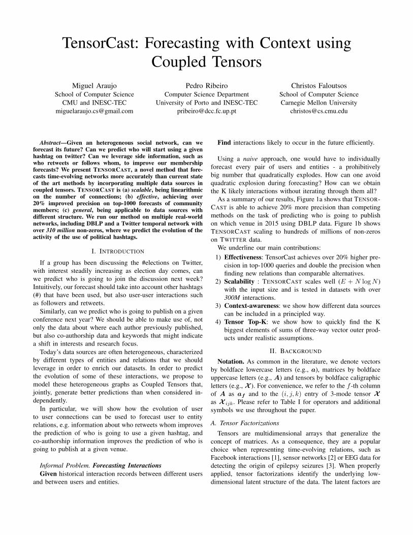
As a summary of our results, Figure 1a shows that TENSOR-CAST is able to achieve 20% more precision than competingmethods on the task of predicting who is going to publishon which venue in 2015 using DBLP data. Figure 1b showsTENSORCAST scaling to hundreds of millions of non-zeroson TWITTER data.

We underline our main contributions:1) Effectiveness: TensorCast achieves over 20% higher pre-

cision in top-1000 queries and double the precision whenfinding new relations than comparable alternatives.

2) Scalability : TENSORCAST scales well (E + N logN )with the input size and is tested in datasets with over300M interactions.

3) Context-awareness: we show how different data sourcescan be included in a principled way.

4) Tensor Top-K: we show how to quickly find the Kbiggest elements of sums of three-way vector outer prod-ucts under realistic assumptions.

II. BACKGROUND

Notation. As common in the literature, we denote vectorsby boldface lowercase letters (e.g., a), matrices by boldfaceuppercase letters (e.g., A) and tensors by boldface caligraphicletters (e.g., X ). For convenience, we refer to the f -th columnof A as af and to the (i, j, k) entry of 3-mode tensor Xas X ijk. Please refer to Table I for operators and additionalsymbols we use throughout the paper.

A. Tensor Factorizations

Tensors are multidimensional arrays that generalize theconcept of matrices. As a consequence, they are a popularchoice when representing time-evolving relations, such asFacebook interactions [1], sensor networks [2] or EEG data fordetecting the origin of epilepsy seizures [3]. When properlyapplied, tensor factorizations identify the underlying low-dimensional latent structure of the data. The latent factors are

0

0.2

0.4

0.6

0.8

1

0 200 400 600 800 1000

Pre

cis

ion

Top-K

Ideal

TensorCast

CP Forecasting

Coupled Matrices

(a) Higher precision when forecasting(author, venue) relations in the DBLP tensor.

0

500

1000

1500

2000

2500

3000

3500

4000

4500

0 M 75 M 150 M 225 M 300 M

Tim

e (

sec)

Input size (non-zeros)

linear

(b) TENSORCAST scales linearly with the number ofnon-zeros.

Fig. 1. TENSORCAST is effective and scalable.

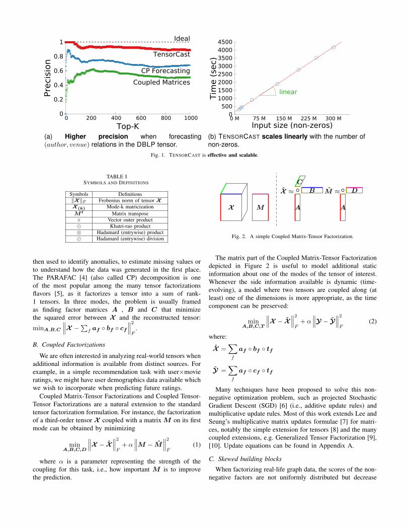
TABLE ISYMBOLS AND DEFINITIONS

Symbols Definitions‖X‖F Frobenius norm of tensor XX (k) Mode-k matricizationMt Matrix transpose◦ Vector outer product� Khatri-rao product⊗ Hadamard (entrywise) product� Hadamard (entrywise) division

then used to identify anomalies, to estimate missing values orto understand how the data was generated in the first place.The PARAFAC [4] (also called CP) decomposition is oneof the most popular among the many tensor factorizationsflavors [5], as it factorizes a tensor into a sum of rank-1 tensors. In three modes, the problem is usually framedas finding factor matrices A , B and C that minimizethe squared error between X and the reconstructed tensor:

minA,B,C

∥∥∥X −∑f af ◦ bf ◦ cf∥∥∥2F

.

B. Coupled Factorizations

We are often interested in analyzing real-world tensors whenadditional information is available from distinct sources. Forexample, in a simple recommendation task with user×movieratings, we might have user demographics data available whichwe wish to incorporate when predicting future ratings.

Coupled Matrix-Tensor Factorizations and Coupled Tensor-Tensor Factorizations are a natural extension to the standardtensor factorization formulation. For instance, the factorizationof a third-order tensor X coupled with a matrix M on its firstmode can be obtained by minimizing

minA,B,C,D

∥∥∥X − X∥∥∥2F+ α

∥∥∥M − M∥∥∥2F

(1)

where α is a parameter representing the strength of thecoupling for this task, i.e., how important M is to improvethe prediction.

X M A

B

C◦X ≈ M ≈

A

D◦

Fig. 2. A simple Coupled Matrix-Tensor Factorization.

The matrix part of the Coupled Matrix-Tensor Factorizationdepicted in Figure 2 is useful to model additional staticinformation about one of the modes of the tensor of interest.Whenever the side information available is dynamic (time-evolving), a model where two tensors are coupled along (atleast) one of the dimensions is more appropriate, as the timecomponent can be preserved:

minA,B,C,T

∥∥∥X − X∥∥∥2F+ α

∥∥∥Y − Y∥∥∥2F

(2)

where:

X =∑f

af ◦ bf ◦ tf

Y =∑f

af ◦ cf ◦ tf

Many techniques have been proposed to solve this non-negative optimization problem, such as projected StochasticGradient Descent (SGD) [6] (i.e., additive update rules) andmultiplicative update rules. Most of this work extends Lee andSeung’s multiplicative matrix updates formulae [7] for matri-ces, notably the simple extension for tensors [8] and the manycoupled extensions, e.g. Generalized Tensor Factorization [9],[10]. Update equations can be found in Appendix A.

C. Skewed building blocks

When factorizing real-life graph data, the scores of the non-negative factors are not uniformly distributed but decrease

sharply. For instance, it has been shown that the internal degreedistribution of big communities can be well approximated bya power-law across several domains [11], that eigenvectorsof Kronecker graphs exhibit a multinomial distribution [12,theorem 3] and multiple generative models where power-law communities arise have been proposed [13], [14], [15].TENSORCAST leverages this property in order to speed-upits computation of Top-K elements without reconstructing theforecasted tensor.

To further strengthen the ubiquity of these structures, Figure3 shows the scores of 4 factors of the venue component of anon-negative factorization of the DBLP author × venue× year tensor we use in the experiments section. Note theskewness of the these scores and that they can be upper-bounded by a power-law.

0.001

0.01

0.1

1

1 10 100 1000 10000

Score

Rank

Factor 1

Factor 2

Factor 3

Factor 4

Fig. 3. Scores of the factor vectors are highly skewed. Non-negativefactorization of the DBLP author × venue × year tensor. Note thelogarithmic scale in both axis.

III. RELATED WORK

A. Top-K elements in Matrix Products

Given the widespread applications of matrix factorizations,finding the top-K elements of a matrix product is an impor-tant problem with several use cases, from personalized userrecommendations to document retrieval.

The problem can be stated as, given matrices A and Bof sizes N × F and M × F , respectively, find the topK (i, j) pairs of the ABt matrix product. Note that thenaive solution requires O(NMF ) operations, iterating overthe (originally) implicitly defined reconstruction matrix. Someattention has been given to this problem, since Ram andGray [16] proposed the use of Cone Trees to speed-up thissearch. Other approaches map this problem into smaller setsof cosine-similarity searches [17], a related but easier problemgiven the unit-length of the vectors. Approximate methodshave also been tried, such as transforming the problem ina near-neighbor search and using locality sensitive hashing(LSH) [18], [19]. However, this is a non-convex optimizationproblem in general.

B. Link Prediction

A large body of literature on link prediction has been createdsince its introduction [20]. In structural link prediction, the

original problem, the goal is to predict which links are morelikely to appear in the future given a current snapshot of thenetwork under analysis. This setting, where it is typical toassume that links are never or seldom removed, has foundmultiple applications in predicting interactions in protein-protein networks, social networks (e.g., friendship relations)and recommendation problems. The Netflix challenge sprungthe creation of several latent factor models with differingstructure and/or regularization terms for this task [21], [22], butthere were also several approaches which showed that usingthe age of the link could lead to improved predictions [23].

On the other hand, given the increased availability ofdynamic or time-evolving graphs (frequently used to modelevolving relationships between entities over time), temporallink prediction methods have been developed to predict futuresnapshots. In this setting where links are not guaranteed topersist over time, we distinguish methods that rely on collaps-ing (matricizing) the input data (e.g., exponential decay ofedge weights [24], [25]) from methods that deal directly withthe increased dimensionality, such as tensor-based methods.CP Forecasting [26] finds a low-rank PARAFAC factorizationand forecasts the time-component in order to incorporateseasonality. TriMine [27] similarly factorizes the input tensor,but then applies probabilistic inference in order to identifyhidden topics that connect users and entities, which it thendraws from in order to generate realistic sequences of futureevents. These methods are not able to integrate contextualinformation on their predictions. Other approaches integratestructure and content in the same prediction task, e.g. Gaoet al [25] suggest a coupled matrix factorizations and graphregularization technique to obtain the latent factors after anexponential decay of the temporal network.

However, none of these methods fulfills all the requirementsfor forecasting when contextual information is considered.Table II contrasts TENSORCAST against the state of the artcompetitors on key specs: (a) linear scalability with sparsedata; (b) interpretability of the underlying model; (c) time-awareness for forecasting periodic, growing and/or decayingrelations; (d) ability to deal with additional contextual in-formation; (e) the ability to forecast the disappearance ofexisting relations; and (f) the ability of providing an orderedranking of future events by likelihood of occurrence.

IV. PROPOSED: TENSORCAST

We assume a coupled-tensors setting where multiple tensors,possibly with different dimensions, are related by commonmodes. We will assume that at least one of these tensors isour tensor of interest: it is a 3-dimensional binary tensor andone of the modes corresponds to a time component which wewould like to forecast.

There are many scenarios that can be instantiated under thissetting: imagine the existence of membership records of theform (user, topic, time), with N unique users and M uniquetopics (or communities) over T unique time intervals encodedin a 3rd-order tensorX ∈ {0, 1}N×M×T . Maybe we also haveavailable an additional collection of user interaction records of

TABLE IITENSORCAST INTEGRATES CONTEXT AND TIME-AWARENESS.

Property Trun

cated

SVD

Trun

cated

Katz

Couple

dM

atrice

s (e.g.,

[25]

)

VAR[28]

, ARIMA[2

9], etc

.

CPFo

recas

ting

[26]

TriM

ine[2

7]

TENSORCAST

Scalability " " " " " "

Interpretability " " " " " "

Coupled setting " "

Time-awareness " " " "

Context-awareness " "

Forecasting " " " "

Ordered Forecasting " " "

the form (user, user, time), similarly encoded in a 3rd-ordertensor Y ∈ {0, 1}N×N×T . One possible forecasting problemcould be framed as predicting which users will interact withwhich topics in the future, taking advantage of the informationfrom both sources1.

We are interested in the following general problem:

Problem 1. Forecasting Tensor EvolutionGiven two coupled tensors (X and Y), a number of K relationsand S time-steps.Forecast, for the next S time-steps, the ranked list of K likelynon-zero elements of X .

While Problem 1 is interesting by itself, accurate top-Kpredictions can often be made by identifying which non-zerosconstantly appear in the tensor of interest. In the previousexample, these would correspond to users that have constantlydiscussed the same topics over time. Therefore, we define thefollowing related problem:

Subproblem 1. Forecasting Novel RelationsGiven two coupled tensors (X and Y), a number of K relationsand S time-steps.Forecast, for the next S time-steps, the ranked list of K likelynew relations of X .

We define a new or novel relation as a non-zero that doesnot exist in the tensor of interest when the time componentis collapsed. We argue that subproblem 1 is more useful inmany realistic scenarios where predicting who is joining orleaving a community is more relevant than predicting who isstaying. For instance, in the elections example, members whorecently joined the discussion are probably easier to influence,while forecasting clients likely to stop doing business with acompany is one of the key problems in customer relations.

Overview. TENSORCAST is comprised of three successivesteps, described in more detail in the following subsections:

1) Non-negative Coupled Factorization: the factorizationwill tie together the various input tensors and identify

1One of the experiments in Section V deals with this scenario.

their rank-1 components.2) Forecasting: given the low dimensional space identified,

we use standard techniques to forecast the time compo-nent.

3) Top-K elements: we exploit the factorization structureand identify the top elements without having to recon-struct the prohibitively big future tensor.

Figure 4 illustrates the intuition of our method.

A. Non-negative Coupled Factorization

Consider that the tensor of interest, X , is a 3-dimensionalN ×M ×T dataset and that the time component correspondsto the last index of the tensor. Then, naively, the number ofelements to be forecasted (S×N×M ) is a prohibitive numberwhen we consider X to be big and sparse.

Therefore, factorizing the input data achieves a two-foldobjective: not only does it reduces the number of elementsto be forecasted, but perhaps more importantly, it co-clusterssimilar elements together enabling generalization. A carefulfactorization will allow the forecast of previously unseenrelations. We opted for a non-negative coupled factorizationin order to improve the interpretability of the model; the im-portance of this feature will be clear when analyzing empiricalevidence in Section V.

We explore how user interactions can be leveraged toimprove forecasts of future user-entity relations. Under thisassumption, the problem is better modeled as two coupledtensors where tensor Y is a N ×N × T symmetric tensor. Inorder to guarantee convergence, we modify the update of thesymmetric factor matrix to

A← A⊗ 3

√X (1)(B � T ) + αY(1)(A� T )

A(B � T )t(B � T ) + αA(A� T )t(A� T )

See Appendix A for further details.

B. Forecasting

Let T be the T×F factor matrix obtained from the previousstep that corresponds to the time component. It consists of a

Yus

ers

users

time

X

user

s

topics

time

T

futu

re

factors

time

Factorize arbitrary set ofcoupled input tensors.

X

user

s

topics

time

Forecasttime factors.

Future tensor is

never fully reconstructed.

Top-K values.

Fig. 4. Overview of TENSORCAST.

small set of F dense factor vectors, hence easy to forecast,that will provide an approximation X of the next time-step.

The most appropriate forecasting mechanism is data-dependent. We forecast using basic exponential smoothing(Holt’s method), but other methods can be applied, e.g. Holt-Winters double exponential smoothing when seasonality ispresent.

C. Tensor Top-K elements

The forecast of the next time-step is a N ×M × S tensorrepresented as

∑f

af ◦ bf ◦ sf where A is N × F , B is

M × F and S is S × F .We extend the literature on the retrieval of maximum entries

in a matrix product to the tensor case, leveraging the fact thatthe factorization was not performed on random data but on agraph that follows typical properties. The goal is to identifythe K (i, j, k) positions with highest value∑

f

AifBjfSkf

We’ll start by showing how this could be achieved if the Xtensor was rank-1 and how multiple factors can be combinedwhile preserving performance guarantees. We assume that thenumber of forecasted time-steps is significantly smaller thanthe number of users or topics (i.e., S � N,M ) and that thenumber of topics is of the same order of magnitude but smallerthan the number of users (i.e., M < N ).

Top-K of single factor. We start by creating a data structurethat lets us obtain the next biggest element in O(log(SM))time, with only O(S logS + M logM + N logN + SM)preprocessing.

Firstly, we sort the three vectors (s, a and b) in decreasingorder. Note that, now, not only do we know that the biggestelement is given by a1b1s1, but also that an element aibjskonly needs to be considered after ai−1bjsk, aibj−1sk andaibjsk−1 have all been identified as one of the biggest K 2.Hence, we can create a priority queue which only holds, atmost, O(SM) elements at a time.

2For instance, we know that the second biggest element is one of a2b1s1,a1b2s1 or a1b1s2.

Combining multiple factors. The major hurdle is handlingthe interaction between multiple factors. We propose a greedyTop-K selection algorithm that, under realistic scenarios, effi-ciently achieves this goal. Algorithm 1 illustrates the pseudocode of this procedure.

We keep a list (R) of the K biggest positions evaluated sofar and Fi.next represents the next element not yet consideredin factor’s i priority queue, as described in the previoussection. In each iteration, we consider the element with thehighest score in one of the factors and add it to the list afterevaluating it across all the factors. We terminate when the sumof the next best scores on each factor becomes smaller thanthe Kth biggest element in R.

input : F - priority queues of factorsinput : K - number of elementsoutput: R - set of biggest elements

1 while∑i Fi.next.factorScore ≤ R.last.Score do

2 f ← argmaxi(Fi.next.factorScore)3 element ← Ff .next4 Ff .pop5 R← R ∪ element.fullScore6 if R.size > K then7 R← R− argmin(R)8 end9 end

10 return RAlgorithm 1: TENSORCAST Top-K Elements

In the following, we prove the correctness and upper boundson the overall number of elements that need to be evaluated.

Theorem 1. Algorithm 1 always returns the correct set ofTop-k elements.

Proof. Consider an element x that should be included in Rbut was never considered. As the algorithm has terminated, itfollows that x’s score is lower than the sum of all the individualfactor scores of elements at the top of each priority queue.However, we know that the smallest element in R is biggerthan this, so this is a contradiction and x cannot exist.

Theorem 1 proves that Algorithm 1 always finds the correctset of elements. We now show that the set of elements thatneed to be considered is small when factors follow commonpower-law distributions. We assume a and b follow power-laws of the form (α− 1)x−α for x ≥ 1 and α > 1.

Lemma 1. If factor vectors a and b follow power-laws withexponents αa and αb, then a randomly drawn element fromany rank-1 frontal slice created as Ckf = a◦b asymptoticallyfollows a power-law

pC(z) = (α− 1)z−α

where α = min(αa, αb).

Proof. Let X and Y follow power-law distributions of theform

pX(x) = (αa − 1)x−αa

pY (y) = (αb − 1)y−αb

Then Z = XY has probability distribution [30, p. 109]:

pZ(z) =

∫ z

1

pX(w)pY

( zw

) 1

wdw =

=(αa − 1)(αb − 1)

αa − αb(z−αa − z−αb)

which tends to a power-law with exponent −min(αa, αb).

Lemma 1 shows that elements randomly drawn from anyrank-1 frontal slice follow a power-law distribution. However,please note that Algorithm 1 iterates over these elements indecreasing order, i.e., deterministically. Therefore, any uncer-tainty is not related to sampling from the distribution, butrather to the skewness of the factor vectors - how well thepower-law assumption holds. Refer back to II-C for furtherdetails and both theoretical and empirical evidence.

Theorem 2. Algorithm 1 needs to check at most KSF 1+ 1α

elements if every frontal slice af ◦ bf follows a power-law.

Proof. We’ll consider the frontal slices one at a time and showthat one only needs to check KF 1+ 1

α elements to find the Kbiggest values of each slice. Let α1..F be the exponents of thepower-law of each of the F factor matrices af ◦bf of a givenfrontal slice and let αm = minα.

The K-th biggest element of∑f af ◦bf is at least K−αm , as

that is the Kth biggest value of the slowest decreasing power-law3. Given the iterative nature of Algorithm 1, we will provean upper-bound for the maximum position (i.e., how deep inone of the factors) an element can be, while still having areconstruction value greater than K−αm . Let x be the positionof such element4, then

K−αm ≤∑f

x−αf ≤ Fx−αm =⇒ x ≤ KF1αm

3Remember that A and B are non-negative matrices. In the worst-case,the score of the Kth biggest element is taken from a single power-law andthe contribution of the rest of the factors is 0, hence K−αm is a lower-boundfor the Kth biggest value.

4In the worst case scenario, this element is at position x in every of thefactors.

This means that any top-k element needs to be in a positionsmaller than KF

1αm in at least one of the factors, which

implies that, in the worst case, Algorithm 1 only needs tocheck KF

1αm F = KF 1+ 1

αm elements to find the K biggestelements on each frontal slice. Therefore, we can upper-boundthe total number of elements checked by KSF 1+ 1

α .

Note that TENSORCAST is linear on the number of elementswe want to obtain times the number of time-steps forecasted.Furthermore, note that this result agrees with intuition: sharper(i.e., quickly decreasing, higher exponent) power-laws requireless elements to be checked, while near-clique factors implylower exponents and more elements to be analyzed.

Figure 5 provides further empirical evidence of the lineargrowth on the number of values we need to check. We plotthe number of positions evaluated as K is increased, on asynthetic network, when forecasting one time-step (S = 1),using 8 factors and varying the power-law exponents from 1.5to 2.2.

1000

10000

100000

1e+06

1e+07

1000 10000 100000

Posit

ions E

valu

ate

d

K

Thm 4.2 (Upperbound)

Measured

Fig. 5. TENSORCAST only checks a linear number of elements of thetensor.

D. Complexity Analysis.

Observation 1. TENSORCAST requires time linear on thenumber of non-zeros of its input tensors.

Rationale. TENSORCAST’s time complexity is a sum of itsthree stages:

1) The coupled-factorization requires linear time on thenumber of non-zeros.

2) Forecasting is typically linear on the number of timesteps,although it depends on the algorithm selected.

3) As shown in the previous section, identifying the top-Kelements is linear on K and sub-quadratic on the numberof factors.

V. EXPERIMENTS

We report experiments to answer the following questions:Q1. Scalability: How fast is TENSORCAST?Q2. Effectiveness and Context-awareness: How does TEN-

SORCAST’s precision compare with its alternatives? Howmuch improvement does contextual data bring?

Q3. Trend Following: How capable is TENSORCAST ofdetecting and following trends?

TABLE IIISUMMARY OF REAL-WORLD NETWORKS USED.

Users Groups Timesteps Memberships Interactions Description1 734 902 5 476 79 8 049 559 21 423 244 DBLP - venues published

and co-authorships.12 426 133 2 326 843 31 30 281 817 282 280 158 TWITTER - hashtags used

and retweets.

Q4. Precision over Time: How does TENSORCAST’s preci-sion decrease as we forecast farther to the future?

TENSORCAST is tested on two big datasets detailed inTable III. In the DBLP dataset, the tensor to be forecastedconsists of authors and venues in which they published from1970 to 2014, while the co-authorship tensor is used ascontextual information. Evaluation is performed on the 2015author × venue data. In the TWITTER dataset, the tensor ofinterest relates users and hashtags (#) they used from Juneto December 2009, while the auxiliary tensor represents userinteractions through re-tweets. Tweets are grouped by weekand evaluation is performed on week 51.

Unless otherwise specified, every factorization approachuses 10 factors. On the TWITTER dataset, we weighted thereconstruction of the tensor of interest as 20 times morerelevant that the context tensor. On DBLP, we weightednon-zeros of the tensor of interest 2.66 times higher thanin the tensor of interest (so that both tensors have the samereconstruction error when considering empty factors).

Q1 - Scalability

We start by evaluating our method’s scalability when chang-ing the number of non-zeros in the TWITTER dataset5. Bychanging the number of weeks under consideration, we createa sequence of pairs of tensors that increase in size. For eachpair, we measure wall-clock time when performing a rank-4coupled tensor factorization, forecasting and identification ofthe top-1000 forecasted non-zeros. Figure 1b shows TENSOR-CAST’s linear scalability.

Q2 - Effectiveness and Context-awareness

Figures 1a and 6 showcase TENSORCAST’s accuracy onthe task of predicting relations on future time steps. WhileFigure 1a shows TENSORCAST’s superior precision as weincrease K on the DBLP dataset, Figure 6 focus particularlyon forecasting novel relations on TWITTER. We would liketo highlight the difficulty of this task, as we are predictingwhether a given user is going to start using a new hashtag onthe next week. Nevertheless, TENSORCAST achieves doublethe precision of competing methods6.

Furthermore, note the importance of TENSORCAST’s abilityof being simultaneously contextual and time-aware, as the

5We consider the sum of the non-zeros of both tensors.6Note that the quality of absolute precision numbers is affected by 1)

how imbalanced the two classes are and 2) the cost of false positives. Animprovement from 2% to 5% precision might imply that 1 out of 20 phone-calls we make target a potential customer versus every 1 in 50.

precision of the current state-of-the-art is limited due toignoring either one of these aspects.

The competing CP Forecasting [26] method was run usingHolt forecasting, given the lack of seasonality of the data.The results of the other competitor, Coupled Matrices, wereobtained by finding non-negative factors that minimize thereconstruction error of the collapsed tensors, weighted for thesame importance. For fairness, all appropriate methods use 10as the number of factors.

0

0.02

0.04

0.06

0.08

0.1

0 2000 4000 6000 8000 10000

Pre

cis

ion

Top-K

2x

Coupled Matrices

CP Forecasting

TensorCast

Fig. 6. Double precision when forecasting novel (user, hashtag) relationsin the TWITTER tensor.

Q3 - Trend Following

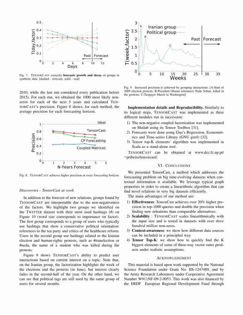
We evaluate TENSORCAST’s ability of predicting an in-crease or decrease in the activity around a given topic orbetween a group of users over time. We created a syntheticdataset with 5 hyperbolic communities (i.e., with power-lawinternal degree distribution) of 100 users over 11 days (10days are used for the factorization and 1 for evaluation). Theaverage density over the first 10 days equals 15% for allcommunities, but their density changes differently over time:two communities have their densities increasing at 1% and2% per day, one has constant density and the other have theirdensity decreasing by 1% and 2% per day.

Figure 7 shows the scores of the 5 columns of the T matrixafter factorization, one per line. We can see that linear changesin density correspond to linear changes of the scores andthat TENSORCAST correctly forecasts a similar change in thefuture.

Q4 - Precision over Time

We evaluate TENSORCAST’s precision as the forecastinghorizon is increased. We use the DBLP dataset, doing fiveruns with each method when considering different “training”periods (i.e., the first run considered every publication before

0

0.1

0.2

0.3

0.4

0.5

0 2 4 6 8 10 12

T(d

ay,f

acto

r)

Days

Past Forecast

Fig. 7. TENSORCAST correctly forecasts growth and decay of groups insynthetic data. [dashed - forecast; solid - real]

2010, while the last run considered every publication before2015). For each run, we obtained the 1000 most likely non-zeros for each of the next 5 years and calculated TEN-SORCAST’s precision. Figure 8 shows, for each method, theaverage precision for each forecasting horizon.

0

0.2

0.4

0.6

0.8

1

0 1 2 3 4 5 6

Pre

cis

ion

N-Years Forecast

Ideal

TensorCast

CP Forecasting

Coupled Matrices

Fig. 8. TENSORCAST achieves higher precision at every forecasting horizon.

Discoveries - TensorCast at work

In addition to the forecast of new relations, groups found byTENSORCAST are interpretable due to the non-negativenessof the factors. We highlight two groups we identified onthe TWITTER dataset with their most used hashtags (#) onFigure 10 (word size corresponds to importance on factor).The first group corresponds to a group of users who typicallyuse hashtags that show a conservative political orientation:references to the tea party and critics of the healthcare reform.Users in the second group use hashtags related to the Iranianelection and human-rights protests, such as #iranelection or#neda, the name of a student who was killed during theprotests.

Figure 9 shows TENSORCAST’s ability to predict userinteractions based on current interest on a topic. Note that,on the Iranian group, the factorization highlights the week ofthe elections and the protests (in June), but interest clearlyfades in the second-half of the year. On the other hand, wecan see that political tags are still used by the same group ofusers for several months.

0

0.5

1

1.5

2

2.5

3

0 5 10 15 20 25 30 35

T(w

eek,f

acto

r)

Weeks

Past Forecast

A

B

C

Iranian group

Political group

Fig. 9. Increased precision is achieved by grouping interactions. [A-Start of2009 election protests; B-President Obama references Neda Soltan, killed inthe protests; C-Taxpayer March in Washington]

Implementation details and Reproducibility. Similarly toits logical steps, TENSORCAST was implemented as threedifferent modules run in succession:

1) The non-negative coupled factorization was implementedon Matlab using its Tensor Toolbox [31].

2) Forecasts were done using Gnu’s Regression, Economet-rics and Time-series Library (GNU gretl) [32].

3) Tensor top-K elements’ algorithm was implemented inScala as a stand-alone tool.

TENSORCAST can be obtained at www.dcc.fc.up.pt/∼pribeiro/tensorcast/.

VI. CONCLUSIONS

We presented TensorCast, a method which addresses theforecasting problem on big time-evolving datasets when con-textual information is available. We leverage typical graphproperties in order to create a linearithmic algorithm that canfind novel relations in very big datasets efficiently.

The main advantages of our method are:1) Effectiveness: TensorCast achieves over 20% higher pre-

cision in top-1000 queries and double the precision whenfinding new releations than comparable alternatives.

2) Scalability : TENSORCAST scales linearithmically withthe input size and is tested in datasets with over threehundred million non-zeros.

3) Context-awareness: we show how different data sourcescan be included in a principled way.

4) Tensor Top-K: we show how to quickly find the Kbiggest elements of sums of three-way vector outer prod-ucts under realistic assumptions.

ACKNOWLEDGMENT

This material is based upon work supported by the NationalScience Foundation under Grant No. IIS-1247489, and bythe Army Research Laboratory under Cooperative AgreementNumber W911NF-09-2-0053. This work was also financed bythe ERDF European Regional Development Fund through

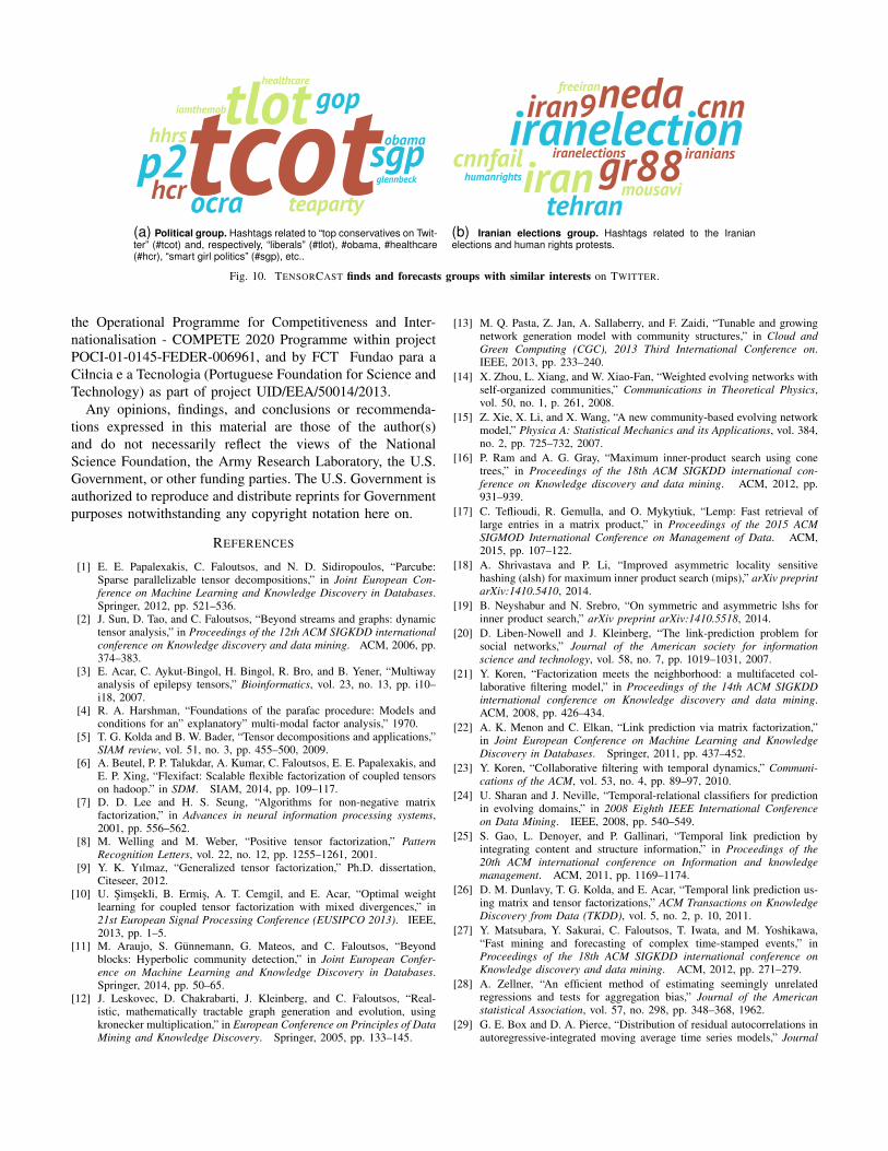
(a) Political group. Hashtags related to “top conservatives on Twit-ter” (#tcot) and, respectively, “liberals” (#tlot), #obama, #healthcare(#hcr), “smart girl politics” (#sgp), etc..

(b) Iranian elections group. Hashtags related to the Iranianelections and human rights protests.

Fig. 10. TENSORCAST finds and forecasts groups with similar interests on TWITTER.

the Operational Programme for Competitiveness and Inter-nationalisation - COMPETE 2020 Programme within projectPOCI-01-0145-FEDER-006961, and by FCT Fundao para aCiłncia e a Tecnologia (Portuguese Foundation for Science andTechnology) as part of project UID/EEA/50014/2013.

Any opinions, findings, and conclusions or recommenda-tions expressed in this material are those of the author(s)and do not necessarily reflect the views of the NationalScience Foundation, the Army Research Laboratory, the U.S.Government, or other funding parties. The U.S. Government isauthorized to reproduce and distribute reprints for Governmentpurposes notwithstanding any copyright notation here on.

REFERENCES

[1] E. E. Papalexakis, C. Faloutsos, and N. D. Sidiropoulos, “Parcube:Sparse parallelizable tensor decompositions,” in Joint European Con-ference on Machine Learning and Knowledge Discovery in Databases.Springer, 2012, pp. 521–536.

[2] J. Sun, D. Tao, and C. Faloutsos, “Beyond streams and graphs: dynamictensor analysis,” in Proceedings of the 12th ACM SIGKDD internationalconference on Knowledge discovery and data mining. ACM, 2006, pp.374–383.

[3] E. Acar, C. Aykut-Bingol, H. Bingol, R. Bro, and B. Yener, “Multiwayanalysis of epilepsy tensors,” Bioinformatics, vol. 23, no. 13, pp. i10–i18, 2007.

[4] R. A. Harshman, “Foundations of the parafac procedure: Models andconditions for an” explanatory” multi-modal factor analysis,” 1970.

[5] T. G. Kolda and B. W. Bader, “Tensor decompositions and applications,”SIAM review, vol. 51, no. 3, pp. 455–500, 2009.

[6] A. Beutel, P. P. Talukdar, A. Kumar, C. Faloutsos, E. E. Papalexakis, andE. P. Xing, “Flexifact: Scalable flexible factorization of coupled tensorson hadoop.” in SDM. SIAM, 2014, pp. 109–117.

[7] D. D. Lee and H. S. Seung, “Algorithms for non-negative matrixfactorization,” in Advances in neural information processing systems,2001, pp. 556–562.

[8] M. Welling and M. Weber, “Positive tensor factorization,” PatternRecognition Letters, vol. 22, no. 12, pp. 1255–1261, 2001.

[9] Y. K. Yılmaz, “Generalized tensor factorization,” Ph.D. dissertation,Citeseer, 2012.

[10] U. Simsekli, B. Ermis, A. T. Cemgil, and E. Acar, “Optimal weightlearning for coupled tensor factorization with mixed divergences,” in21st European Signal Processing Conference (EUSIPCO 2013). IEEE,2013, pp. 1–5.

[11] M. Araujo, S. Gunnemann, G. Mateos, and C. Faloutsos, “Beyondblocks: Hyperbolic community detection,” in Joint European Confer-ence on Machine Learning and Knowledge Discovery in Databases.Springer, 2014, pp. 50–65.

[12] J. Leskovec, D. Chakrabarti, J. Kleinberg, and C. Faloutsos, “Real-istic, mathematically tractable graph generation and evolution, usingkronecker multiplication,” in European Conference on Principles of DataMining and Knowledge Discovery. Springer, 2005, pp. 133–145.

[13] M. Q. Pasta, Z. Jan, A. Sallaberry, and F. Zaidi, “Tunable and growingnetwork generation model with community structures,” in Cloud andGreen Computing (CGC), 2013 Third International Conference on.IEEE, 2013, pp. 233–240.

[14] X. Zhou, L. Xiang, and W. Xiao-Fan, “Weighted evolving networks withself-organized communities,” Communications in Theoretical Physics,vol. 50, no. 1, p. 261, 2008.

[15] Z. Xie, X. Li, and X. Wang, “A new community-based evolving networkmodel,” Physica A: Statistical Mechanics and its Applications, vol. 384,no. 2, pp. 725–732, 2007.

[16] P. Ram and A. G. Gray, “Maximum inner-product search using conetrees,” in Proceedings of the 18th ACM SIGKDD international con-ference on Knowledge discovery and data mining. ACM, 2012, pp.931–939.

[17] C. Teflioudi, R. Gemulla, and O. Mykytiuk, “Lemp: Fast retrieval oflarge entries in a matrix product,” in Proceedings of the 2015 ACMSIGMOD International Conference on Management of Data. ACM,2015, pp. 107–122.

[18] A. Shrivastava and P. Li, “Improved asymmetric locality sensitivehashing (alsh) for maximum inner product search (mips),” arXiv preprintarXiv:1410.5410, 2014.

[19] B. Neyshabur and N. Srebro, “On symmetric and asymmetric lshs forinner product search,” arXiv preprint arXiv:1410.5518, 2014.

[20] D. Liben-Nowell and J. Kleinberg, “The link-prediction problem forsocial networks,” Journal of the American society for informationscience and technology, vol. 58, no. 7, pp. 1019–1031, 2007.

[21] Y. Koren, “Factorization meets the neighborhood: a multifaceted col-laborative filtering model,” in Proceedings of the 14th ACM SIGKDDinternational conference on Knowledge discovery and data mining.ACM, 2008, pp. 426–434.

[22] A. K. Menon and C. Elkan, “Link prediction via matrix factorization,”in Joint European Conference on Machine Learning and KnowledgeDiscovery in Databases. Springer, 2011, pp. 437–452.

[23] Y. Koren, “Collaborative filtering with temporal dynamics,” Communi-cations of the ACM, vol. 53, no. 4, pp. 89–97, 2010.

[24] U. Sharan and J. Neville, “Temporal-relational classifiers for predictionin evolving domains,” in 2008 Eighth IEEE International Conferenceon Data Mining. IEEE, 2008, pp. 540–549.

[25] S. Gao, L. Denoyer, and P. Gallinari, “Temporal link prediction byintegrating content and structure information,” in Proceedings of the20th ACM international conference on Information and knowledgemanagement. ACM, 2011, pp. 1169–1174.

[26] D. M. Dunlavy, T. G. Kolda, and E. Acar, “Temporal link prediction us-ing matrix and tensor factorizations,” ACM Transactions on KnowledgeDiscovery from Data (TKDD), vol. 5, no. 2, p. 10, 2011.

[27] Y. Matsubara, Y. Sakurai, C. Faloutsos, T. Iwata, and M. Yoshikawa,“Fast mining and forecasting of complex time-stamped events,” inProceedings of the 18th ACM SIGKDD international conference onKnowledge discovery and data mining. ACM, 2012, pp. 271–279.

[28] A. Zellner, “An efficient method of estimating seemingly unrelatedregressions and tests for aggregation bias,” Journal of the Americanstatistical Association, vol. 57, no. 298, pp. 348–368, 1962.

[29] G. E. Box and D. A. Pierce, “Distribution of residual autocorrelations inautoregressive-integrated moving average time series models,” Journal

of the American statistical Association, vol. 65, no. 332, pp. 1509–1526,1970.

[30] G. Grimmett and D. Stirzaker, Probability and random processes.Oxford university press, 2001.

[31] B. W. Bader, T. G. Kolda et al., “Matlab tensor toolbox version2.6,” Available online, February 2015. [Online]. Available: http://www.sandia.gov/∼tgkolda/TensorToolbox/

[32] G. Baiocchi and W. Distaso, “Gretl: Econometric software for the gnugeneration,” Journal of applied econometrics, vol. 18, no. 1, pp. 105–110, 2003.

[33] Z. He, S. Xie, R. Zdunek, G. Zhou, and A. Cichocki, “Symmetricnonnegative matrix factorization: Algorithms and applications to prob-abilistic clustering,” IEEE Transactions on Neural Networks, vol. 22,no. 12, pp. 2117–2131, 2011.

[34] B. Ermis, A. T. Cemgil, and E. Acar, “Generalized coupled symmetrictensor factorization for link prediction,” in Signal Processing andCommunications Applications Conference (SIU), 2013 21st. IEEE,2013, pp. 1–4.

APPENDIXMULTIPLICATIVE UPDATES OF COUPLED TENSORS

FACTORIZATION

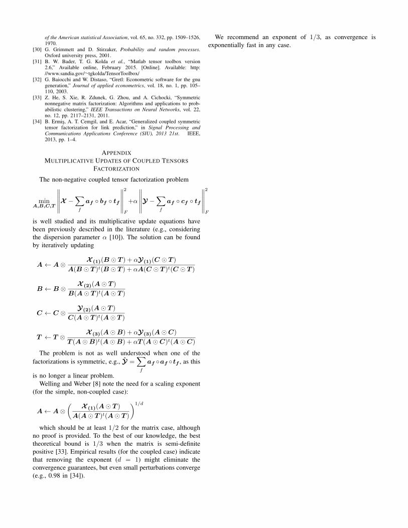
The non-negative coupled tensor factorization problem

minA,B,C,T

∥∥∥∥∥∥X −∑f

af ◦ bf ◦ tf

∥∥∥∥∥∥2

F

+α

∥∥∥∥∥∥Y −∑f

af ◦ cf ◦ tf

∥∥∥∥∥∥2

F

is well studied and its multiplicative update equations havebeen previously described in the literature (e.g., consideringthe dispersion parameter α [10]). The solution can be foundby iteratively updating

A ← A⊗X (1)(B � T ) + αY(1)(C � T )

A(B � T )t(B � T ) + αA(C � T )t(C � T )

B ← B ⊗X (2)(A� T )

B(A� T )t(A� T )

C ← C ⊗Y(2)(A� T )

C(A� T )t(A� T )

T ← T ⊗X (3)(A�B) + αY(3)(A�C)

T (A�B)t(A�B) + αT (A�C)t(A�C)

The problem is not as well understood when one of thefactorizations is symmetric, e.g., Y =

∑f

af ◦af ◦tf , as this

is no longer a linear problem.Welling and Weber [8] note the need for a scaling exponent

(for the simple, non-coupled case):

A← A⊗( X (1)(A� T )A(A� T )t(A� T )

)1/d

which should be at least 1/2 for the matrix case, althoughno proof is provided. To the best of our knowledge, the besttheoretical bound is 1/3 when the matrix is semi-definitepositive [33]. Empirical results (for the coupled case) indicatethat removing the exponent (d = 1) might eliminate theconvergence guarantees, but even small perturbations converge(e.g., 0.98 in [34]).

We recommend an exponent of 1/3, as convergence isexponentially fast in any case.