Magnetic Resonance in Medicine 64:138–148 (2010)

Tensor Kernels for Simultaneous Fiber Model Estimationand Tractography

Yogesh Rathi,1* James G. Malcolm,1 Oleg Michailovich,2 Carl-Fredrik Westin,3

Martha E. Shenton,1,4 and Sylvain Bouix1

This paper proposes a novel framework for joint orientationdistribution function estimation and tractography based on anew class of tensor kernels. Existing techniques estimate thelocal fiber orientation at each voxel independently so there isno running knowledge of confidence in the measured signal orestimated fiber orientation. In this work, fiber tracking is formu-lated as recursive estimation: at each step of tracing the fiber,the current estimate of the orientation distribution function isguided by the previous. To do this, second-and higher-ordertensor-based kernels are employed. A weighted mixture of thesetensor kernels is used for representing crossing and branch-ing fiber structures. While tracing a fiber, the parameters ofthe mixture model are estimated based on the orientation dis-tribution function at that location and a smoothness term thatpenalizes deviation from the previous estimate along the fiberdirection. This ensures smooth estimation along the direction ofpropagation of the fiber.

In synthetic experiments, using a mixture of two and threecomponents it is shown that this approach improves the angularresolution at crossings. In vivo experiments using two and threecomponents examine the corpus callosum and corticospinaltract and confirm the ability to trace through regions knownto contain such crossing and branching. Magn Reson Med64:138–148, 2010. © 2009 Wiley-Liss, Inc.

Key words: diffusion-weighted MRI; tractography; diffusiontensor estimation; high order tensors; spherical harmonics

The advent of diffusion-weighted MRI has provided theopportunity for noninvasive investigation of neural archi-tecture. Using this imaging technique, clinicians and neu-roscientists want to ask how neurons originating from oneregion connect to other regions or how well defined thoseconnections may be. For such studies, the quality of theresults relies heavily on the chosen fiber representation andthe method of reconstructing pathways.

To begin studying the microstructure of fibers, we needa model to interpret the diffusion-weighted signal. Suchmodels fall broadly into two categories: parametric andnonparametric. One of the simplest parametric models is

1Psychiatry Neuroimaging Laboratory, Brigham and Women’s Hospital, Har-vard Medical School, Boston, Massachusetts, USA2Department of Electrical Engineering, University of Waterloo, Canada3Laboratory for Mathematical Imaging, Brigham and Women’s Hospital, Har-vard Medical School, Boston, Massachusetts, USA4VA Boston Healthcare System, Brockton Division, Brockton, Massachusetts,USA*Correspondence to: Yogesh Rathi, Ph.D., Psychiatry Neuroimaging Labora-tory, Brigham and Women’s Hospital, Harvard Medical School, 1249 BoylstonSt, Boston, MA 02215. E-mail: yogesh@bwh.harvard.eduReceived 6 April 2009; revised 30 June 2009; accepted 21 October 2009.DOI 10.1002/mrm.22292Published online in Wiley InterScience (www.interscience.wiley.com).

the diffusion tensor, which describes a gaussian estimate ofthe diffusion orientation and strength at each voxel (1,2).While robust, this model can be inadequate in cases ofmixed fiber presence or more complex orientations (3,4).To handle more complex diffusion patterns, various para-metric models have been introduced: weighted mixtures(5–8), higher-order tensors (9,10) and directional functions(11–13).

Nonparametric models often provide more informationabout the diffusion pattern. Instead of estimating a discretenumber of fibers as in parametric models, nonparametrictechniques estimate an orientation distribution function(ODF) describing an arbitrary configuration of fibers. Forthis estimation, Tuch (14) introduced Q-ball imaging tonumerically compute the ODF (also refered to as diffusion-ODF[dODF]) using the Funk-Radon transform. The use ofspherical harmonics (SH) simplified the computation withan analytic form (15–17). A good review of both parametricand nonparametric models can be found (18,19).

Deterministic tractography involves directly followingthe diffusion pathways. In the single-tensor model, thismeans simply following the principal diffusion direction(20), while multifiber models often include techniques fordetermining the number of fibers present or when path-ways branch (7,21). Since the estimated model at eachlocation is inherently noisy, some methods perform pathregularization using a filtering technique (22).

In order to perform deterministic tractography using non-parametric methods, one has to use a separate algorithmto find the dODF maxima. Since the dODF peaks are verysmooth, the principal diffusion direction obtained from itis very noisy (19). Recent work has focused on estimatingthe fiber-ODF (fODF) either directly from the signal or fromthe dODF (23–25). For example, Bloy and Verma (25) foundthem as maxima on the surface of a high-order tensor andSchultz and Seidel (26) decompose a high-order tensor intoa mixture of rank-1 tensors. Ramirez et al. (27) provide aquantitative comparison of several such techniques.

Another popular technique to estimate the fODF hasbeen to use spherical deconvolution (12,28–32). In thisapproach, a model for the signal response of a single fiberis assumed and the observed signal is deconvolved toobtain the true fODF. This technique sharpens the peak ofthe ODF and it becomes much easier to extract the max-ima. Descoteaux et al. (19) have shown improvement intractography results, with fODF computed using sphericaldeconvolution.

An alternative method is to use a mixture model of direc-tional kernels, each representing a single fiber response.The advantages of the mixture model are that a separatealgorithm is not needed to find the fODF maxima since

© 2009 Wiley-Liss, Inc. 138

High-order Tensor Tractography 139

the kernel parameters include the principal diffusion direc-tion. Further, the scaling parameter can adjust the shape ofthe ODF, i.e., it can adjust the single fiber response based onthe observed data (white matter, gray matter, cerebrospinalfluid, etc.) and hence allows for better model fit for whitematter and gray matter regions. The disadvantage, however,is that the number of fibers (components of mixture model)at each location have to be kept fixed or determined onlineduring estimation.

MATERIALS AND METHODS

In this work, we first propose a novel kernel based onsecond-and higher-order rank-1 tensors. The two param-eters of the kernel determine the orientation and shape(scaling) of the kernel. We will use this tensor kernel torepresent fODF.

Second, while most of the approaches listed above per-form dODF (or fODF) estimation independently at eachvoxel, we describe in this paper a method to estimatethe model parameters and perform tractography simulta-neously as we trace a fiber from its seed to termination. Inthis way, the estimation at each position builds upon theprevious estimates along the fiber.

We use a mixture of two/three components and formulateour cost function in such a way that if there is one fiber, thecomponents of the mixture align in the same general direc-tion and disperse if there is more than one fiber at a givenlocation. Further, we constrain the solution to be consistentwith the model estimated at the previous location.

Using causal estimation in this way yields inherent pathregularization and accurate fiber resolution at crossingangles not found with independent optimization.

APPROACH

In this section, we propose a function using second- andhigher-order tensors capable of representing ODFs andexamine some of their properties. We also define two dif-ferent cost functions, which are minimized in order toestimate the parameters of the mixture model.

Tensor Kernel

One of the goals of this paper is to extract the fODF fromthe dODF. To do this, we need kernels (functions) that canaccurately represent a fODF. Second- and higher-order ten-sors provide a way to represent functions on the sphere (thefODF is a function on the sphere). In this work, we treatorder-l tensors T in a given orthonormal Cartesian coor-dinate system as quantities whose elements are addressedby l indices. The employed tensors are supersymmetric,i.e., their elements Ti1i2...il are invariant under arbitrary per-mutations of indices i1i2 . . . il . A function D(g) on the unitsphere is given by its induced homogeneous form. For anorder-l tensor T in three dimensions, it reads:

D(g) =3∑

i1=1

3∑i2=1

. . . .3∑

il=1

Ti1i2...il gi1 gi2 . . . gil

The above equation can be compactly written using thetensor contraction operator “:”

D(g) = T : Gl , G

l = g ⊗ g ⊗ . . . g︸ ︷︷ ︸l times

, g = [g1 g2 g3]T , [1]

where ⊗ is the outer product operation and Gl is a rank-

1 tensor of order-l. The tensor contraction operator : isan inner product between matrices analogous to an innerproduct between vectors.

Let g1g2 . . . gn ∈ S3 be the directions that represent a uni-form sampling of the sphere. Then, we propose to use thefollowing tensor kernel to represent an ODF with principaldiffusion direction along t:

D(gi) =(T

l : Gli

)p, [2]

where Tl is the order-l tensor of rank-1 in direction t, G

li

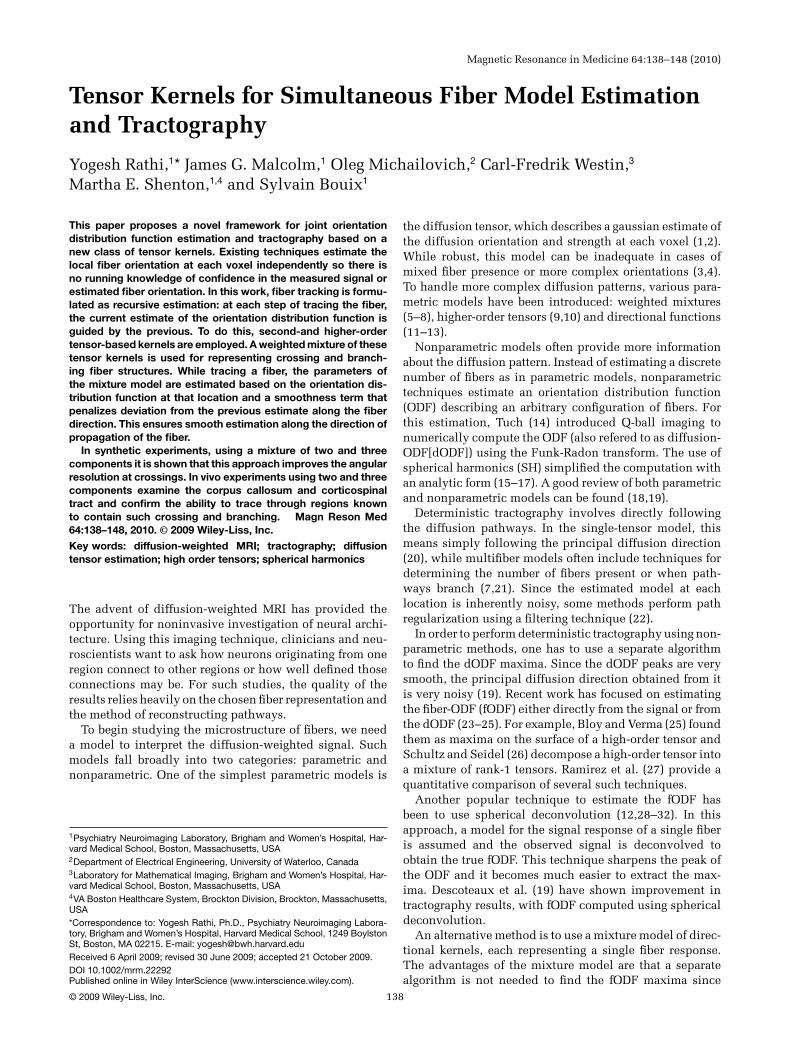
is order-l tensor in direction gi , and p is a scaling param-eter. Note that a particular case of this function has beenused in the literature with p = 1 (26,33). This is, however,the first time we have modified it to have a scaling param-eter, giving more flexibility to represent various kinds ofshapes. Figure 1 shows the effect of the scaling parameterp on the shape of the function. The top row shows the func-tion for order-6, middle for order-4 and bottom for order-2.Thus, we have a family of functions, given by their order,that can represent single-fiber response. The higher-orderkernels differ from their lower-order counterparts in termsof the scaling. Note that we only require three parametersthat can uniquely define the tensor kernel: the principaldiffusion direction t requires two parameters in sphericalcoordinates and one scaling parameter p.

Mixture Model

In diffusion-weighted imaging, image contrast is related tothe strength of water diffusion, and our goal is to accuratelyrelate these signals to an underlying model of fiber orienta-tion. At each image voxel, diffusion is measured along a setof distinct gradients, g1, . . . , gn ∈ S3 (on the unit sphere),producing the corresponding signal, S = [s1, ..., sn]T ∈ Rn.Thus, the signal S is a function defined on the sphere.

A popular method to represent functions on the sphere isusing spherical harmonics (SH) (15–17). Given any band-limited signal S defined on the sphere, one can write itas an expansion in terms of the SH basis as: S(θ , φ) =∑L

l=0∑l

m=−l cl,mYl,m, for any direction (θ , φ), where Yl,m arethe basis functions given by:

Yl,m(θ , φ) =√

(2l + 1)(l − m)!4π (l + m)! Pl,m(cos θ )eimφ ,

and Pl,m is the associated Legendre polynomial. The aboveequations can be written as a linear system of equations andcl,m can be computed using the Moore-Penrose pseudoin-verse. To make the method robust to noise, Descoteaux et al.(17) proposed a regularized version by adding a smoothnessconstraint.

Once the signal representation is obtained in the SHbasis, the corresponding dODF can be analytically com-puted using the Funk-Radon transform (17). This method

140 Y. Rathi et al.

FIG. 1. Tensor kernels of different orders and scales. Top row: order-6; middle: order-4; and bottom: order-2. Left to right: P = 0.5, 1, 2.Red to blue shows higher to lower diffusion values. [Color figure canbe viewed in the online issue, which is available at www.interscience.wiley.com.]

is very fast and robust to noise. In the remainder of thiswork, we will assume that the dODF has been precomputedusing SH (see (17) for details). There has been a lot of workrecently to extract the fODF from dODF using sphericaldeconvolution (12,28–30,32). This method assumes a fixedsingle-fiber response while allowing for variable numbersof fibers to be estimated.

In this work, we seek to estimate the fODF using adifferent strategy by allowing for variation in single-fiberresponse but keeping the number of fibers fixed. This can bedone by fitting the dODF using a mixture of tensor kernels.While one can assume a mixture of any number of compo-nents, we choose to start with a mixture involving two andthree weighted tensor kernels. While the work of Behrenset al. (34) showed that at a b-value of 1000 the maximumnumber of detectable fibers is two, several other studiesrestricted their analysis to two-fiber models due to prob-lems with estimating more than two components (6,7,23).In this work, we perform experiments on synthetic datausing two components and later show an extension to threecomponents. Similar results are shown for in vivo data.

The model we intend to use in this study is given by:

D(gi) =N∑

j=1

wj

(T

lj : G

li

)pj, [3]

where D(gi) is the dODF in direction gi , wj are the respectiveweights of the components, G

li is the lth order rank-1 tensor

obtained from the gradient direction gi , and Tlj is lth order

rank-1 tensor with principal diffusion direction tj . N is thetotal number of components used in the mixture, whichin our case could be two or three. Thus, a two-componentdODF can be uniquely represented using 10 parameters (iftj ∈ R3) or eight parameters if the directions are representedin spherical coordinates. We should also clarify that D is

the dODF but the individual components of the mixturemodel give the fODF in direction tj . The remainder of thissection will focus on estimating the free parameters of thismixture model, i.e., {tj , wj , pj , }N

j=1.

Independent Estimation

Given the scanner signal S ∈ Rn, we compute the corre-sponding dODF F = [F1, F2, . . . Fn] ∈ Rn using SH (17)and min-max normalize it (14). One can now minimize thefollowing cost function to estimate the parameters:

E =n∑

i=1

(Fi − Di)2 =n∑

i=1

Fi −

N∑j=1

wj

(T

lj : G

li

)pj

2

, [4]

where we have used the shorthand notation D(gi) = Di

and F (gi) = Fi . Equation 4 can be minimized using theLevenberg-Marquardt nonlinear optimizer. However, theminimum could be a degenerate solution with negative wj

and/or pj . To overcome this problem, we use the exponen-tial map to guarantee positivity of the weight and scalingparameters (10), i.e., we use wj = exp(−wj ) and pj = exp(pj )in Eq. 4:

E =n∑

i=1

Fi −

N∑j=1

wj

(T

lj : G

li

)pj

2

. [5]

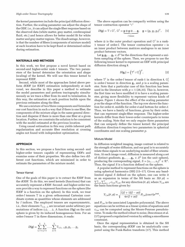
To obtain volume fraction contribution for each compo-nent, one can normalize the weights so that they sum to 1.Figure 2 shows how the individual fODFs combine to givethe observed dODF. Note that maxima of F would not haverevealed the individual fiber composition of the dODF.

Given the signal at each location in the brain, one couldindependently estimate the dODF and the mixture modelparameters, as is done in most of the techniques presentedin the literature. However, in this paper, we make theobservation that the diffusion of water molecules is notindependent and is highly correlated along the directionof the fiber bundle. We will demonstrate that taking thisinto account significantly improves tractography results.

Smooth Estimation and Tractography

In this work, we take this spatial correlation into accountand propose to do simultaneous model estimation and trac-tography. This means we recursively estimate the model

FIG. 2. Mixture components of dODF at an angle of 45◦ [Colorfigure can be viewed in the online issue, which is available at www.interscience.wiley.com.]

High-order Tensor Tractography 141

parameters at location x based on the observed dODF at xand the model parameters estimated at x−1 (previous loca-tion along the fiber tract). Once the model parameters areestimated, we propagate a unit step along the most consis-tent direction. Causal estimation and tracking in this wayallow for smooth and accurate estimation of the fiber.

In order to take into account the estimated model param-eters at the previous location x − 1, we modify the costfunction in Eq. 5:

E(x) =n∑

i=1

Fi(x) −

N∑j=1

wj

(T

lj (x) : G

li

)pj

2

+ λ1

N∑j=1

(wj (x) − wj (x − 1))2 + λ2

N∑j=1

(pj (x) − pj (x − 1))2

+ λ3

N∑j=1

(1 − (

tj (x)T tj (x − 1))2

), [6]

where the first is the data consistency term at location x,and the 2nd, 3rd and 4th terms ensure that the weights, scale,and direction are consistent with the previous estimationat x − 1. The constants λ1, λ2, λ3 are user-defined constantsthat determine the influence of the previous estimate on thecurrent. In our experiments, we empirically obtained theseconstants by choosing the ones that gave the best tractog-raphy results on synthetic data. One could, however, use astrategy that either does a brute force search or minimizesthe error to obtain these constants. We, however, noticedthat the estimation works well for a braod range of val-ues. Eq. 6 can be minimized using an Levenberg-Marquardtoptimizer.

To perform tractography, we repeatedly minimize Eq. 6at each voxel location x and then propagate a unit stepin the most consistent direction. The principal diffusiondirections are given by t1 and t2, and hence there is no needfor a separate peak-finding algorithm. Smooth parameterestimation along the fiber in this way gives significantlybetter results than independent estimation, as is clear fromsynthetic and in vivo results given in the next section. Asummary of the entire algorithm is given below:

1. Compute the dODF using SH (17).2. Min-max normalize the dODF to obtain F (x)3. Minimize Eq. 6 using a Levenberg-Marquardt opti-

mizer to obtain {tj , wj , pj}Nj=1.

4. Move a unit step that is consistent with the incomingdirection, i.e., move a step along t1(x).

5. Stop if the generalized fractional anisotropy (14) isless than 0.05 or if the radius of curvature of the fiberat location x is less than 0.87 or the weight of thecomponent in the direction of propagation is less than40% of the other weight.

6. Otherwise go to step 1 and repeat for position x + 1.

Before we conclude this section, we note some existingtechniques that do spatial regularization during estima-tion (35,36). In Fillard et al. (35), the authors estimate asingle tensor using the log-Euclidean metric, along witha spatial smoothness term. In Assemlal et al. (36), theauthors extend it for smooth estimation of the spherical

harmonic coefficients. Both of these methods assume aspatial neighborhood (3 × 3 × 3) within which the regular-ization is done. However, none of these methods performsimultaneous tractography and estimation in their frame-work (as is proposed in this work).

We also note some techniques that have used mixturemodel to represent ODFs. In recently proposed work (26),the authors use a tensor decomposition approach to find amixture of rank-1 tensors of order-l that best fit the givendODF. Some of the important differences with this methodare as follows: (a) The authors estimate the standard high-order tensor of rank-1 with a single fixed scale (p = 1). Inorder to compensate for the scaling, they deconvolve thedODF using a fixed kernel and map it to an appropriatespace so that a rank-1 order-l tensor can be fit to it. (b) Onceagain, the authors perform an independent estimation ateach voxel location and then do tractography on it. McGrawet al. (11) use a mixture model of von-Mises Fisher functionto estimate an ODF. They also perform independent estima-tion at each voxel and thus ignore the correlation in fibergeometry. Sotiropoulos et al. (37) estimate the parametersof a two-tensor gaussian mixture model using relaxationlabeling as their regularizer.

RESULTS

We first use experiments with synthetic data to validateour technique against ground truth. We confirm that ourapproach reliably recognizes crossing fibers over a broadrange of angles. Comparing against two alternative multi-fiber optimization techniques, we find that the constrainedtractography approach gives consistently superior results.Next, we perform tractography through crossing fiber fieldsand qualitatively examine the underlying orientations andbranchings (see Section Synthetic Tractography). Last, weexamine a real dataset to demonstrate how constrained esti-mation is able to pick up fibers and branchings knownto exist in vivo yet that are undetectable using decon-volved SH and single tensor models (see Section In VivoTractography).

Following the experimental method of generating syn-thetic data (19,26,30), we pull from our real data setthe 300 voxels with highest fractional anisotropy andcompute the average eigenvalues among these voxels:{1200, 100, 100}µm2/msec (fractional anisotropy = 0.91).We generated synthetic MR signals according to a gaussianmixture model, as done in Tuch (14), using these eigen-values to form an anisotropic tensor at both b = 1000 andb = 3000, with 81 gradient directions uniformly spread onthe hemisphere. We generate two separate data sets, eachwith a different level of Rician noise along the fiber direc-tion: low noise (signal-to-noise ratio (SNR) ≈ 10 dB) andhigh noise (SNR ≈ 5 dB).

Throughout the experiments, we draw comparison totwo other independent optimization techniques. In whatfollows, we use the second- and fourth- order tensor ker-nels. First, we use the proposed tensor kernel within themixture model framework but do an independent optimiza-tion using Eq. 5. Second, we use SH for modeling (30)and fODF sharpening with peak detection, as describedin Descoteaux et al. (19) (order l = 6, regularizationL = 0.006). This provides a comparison with an indepen-dently estimated, model-free representation. Last, when

142 Y. Rathi et al.

FIG. 3. Angular error for second-order kernel using constrained opti-mization (blue), independent optimization (red), and sharpened SH(black) for b = 1000. The dotted vertical bars show range of 1 stan-dard deviation. Left: low noise; right: high noise. [Color figure can beviewed in the online issue, which is available at www.interscience.wiley.com.]

performing tractography on real data, we use single-tensorstreamline tractography as a baseline, using the freelyavailable Slicer 2.7 (http://www.slicer.org).

Angular Resolution

While the independent optimization techniques can berun on individually generated voxels, care must be takenin constructing reasonable scenarios to test the causalfilter. For this purpose, we constructed an actual two-dimensional field through which to navigate (see Fig. 9).In the middle is one long fiber pathway where the trackerbegins estimating a single tensor but then runs into a fieldof voxels with two crossed fibers at a fixed angle. Wecomputed the angular error over this region using bothsharpened SH and independent optimization (5). We gen-erated several similar fields, each at a different fixed angle.By varying the size of the crossing region or the numberof fibers run, we ensured that each technique performedestimation on at least 500 voxels.

We looked at the error in angular resolution by comparingthe constrained approach to independent optimization andsharpened SH. For the tensor kernels (two components),we show comparison using both, second- and fourth- ordertensors. Consistent with other results reported in (17,19),sharpened SH are generally unable to detect and resolveangles below 50◦ for b = 1000. Figures 3 and 4 confirmthis.

As expected, the independent optimization techniquealso reports large errors since the Levenberg-Marquardtoptimizer gets stuck in local minimum. For example,any dODF can be represented using a single componentwith significant weight and appropriate scaling parameterwhile rendering the contribution from the other compo-nent to zero by setting the weight to be zero. Such solu-tions contribute to large errors when using independentoptimization.

However, in the constrained estimation technique, weconstrain the weight and the scaling parameter to be close

to its previous estimate, which results in a better estimationof the parameters. For in vivo and synthetic data, the user-defined values of λ1, λ2, λ3 in Eq. 6 were emprirically foundto be 2.5, 1, and 0.15, respectively, for a second-order tensorkernel. Thus, the deviation of the weights from the previousestimate had the largest penalty, the scaling parameter hada little more flexibility, and the penalty on direction param-eter was still lower. Intuitively, for the case of a single fiber,this means that equally weighted, similarly aligned com-ponents are more preferable than a single component withthe correct direction but zero contribution from the secondcomponent. Thus, upon encountering a region of disper-sion, the second component is poised and ready to beginbranching. Overall, the relative weighting of the penaltyterms ensures that there is no abrupt change in either theweight or the scale of the estimated fODF along the fiberbut still allows flexibility to capture fiber crossings at highangles.

This experiment demonstrates that for b = 1000, theconstrained approach consistently resolves angles down to25−30◦ with 5◦ error compared to independent optimiza-tion, which reports very high error for certain angles andsharpened SH, which fails to reliably resolve below 60◦with as much as 15◦ error. For b = 3000, the constrainedapproach consistently resolves down to 20−30◦ with 1−2◦error compared to sharpened SH which cannot resolvebelow 50◦ with 5◦ error (Fig. 5). Further, the angular errorsreported using the constrained optimization with second-and fourth-order tensor kernels are very close, and hencewe will only show in vivo results using the second-ordertensor kernel.

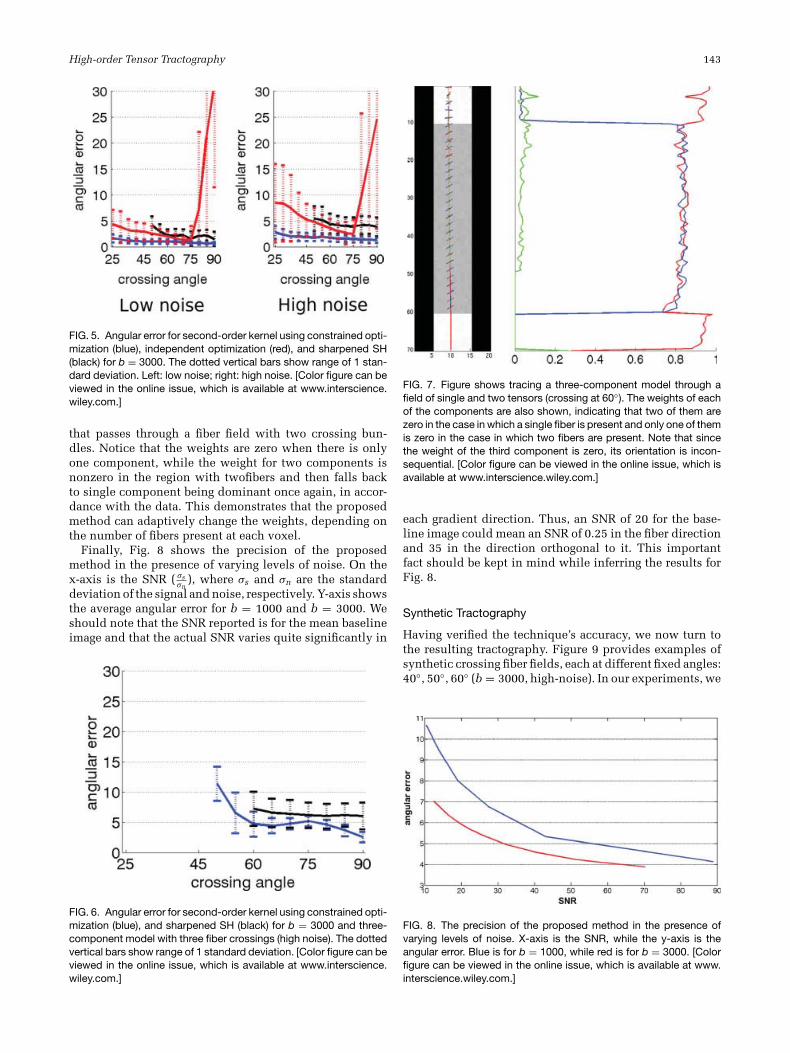
We also performed a similar experiment to test howwell our method performs in the case of three crossingfibers. In this case, we used a mixture of three compo-nents with different crossing angles, as described earlier.Figure 6 demonstrates that the proposed method has lowerangular error than sharpened SH. Figure 7 shows orienta-tion and weights of three components as they trace a fiber

FIG. 4. Angular error for fourth-order kernel using constrained opti-mization (blue), independent optimization (red), and sharpened SH(black) for b = 1000. The dotted vertical bars show range of 1 stan-dard deviation. Left: low noise; right: high noise. [Color figure can beviewed in the online issue, which is available at www.interscience.wiley.com.]

High-order Tensor Tractography 143

FIG. 5. Angular error for second-order kernel using constrained opti-mization (blue), independent optimization (red), and sharpened SH(black) for b = 3000. The dotted vertical bars show range of 1 stan-dard deviation. Left: low noise; right: high noise. [Color figure can beviewed in the online issue, which is available at www.interscience.wiley.com.]

that passes through a fiber field with two crossing bun-dles. Notice that the weights are zero when there is onlyone component, while the weight for two components isnonzero in the region with twofibers and then falls backto single component being dominant once again, in accor-dance with the data. This demonstrates that the proposedmethod can adaptively change the weights, depending onthe number of fibers present at each voxel.

Finally, Fig. 8 shows the precision of the proposedmethod in the presence of varying levels of noise. On thex-axis is the SNR ( σs

σn), where σs and σn are the standard

deviation of the signal and noise, respectively. Y-axis showsthe average angular error for b = 1000 and b = 3000. Weshould note that the SNR reported is for the mean baselineimage and that the actual SNR varies quite significantly in

FIG. 6. Angular error for second-order kernel using constrained opti-mization (blue), and sharpened SH (black) for b = 3000 and three-component model with three fiber crossings (high noise). The dottedvertical bars show range of 1 standard deviation. [Color figure can beviewed in the online issue, which is available at www.interscience.wiley.com.]

FIG. 7. Figure shows tracing a three-component model through afield of single and two tensors (crossing at 60◦). The weights of eachof the components are also shown, indicating that two of them arezero in the case in which a single fiber is present and only one of themis zero in the case in which two fibers are present. Note that sincethe weight of the third component is zero, its orientation is incon-sequential. [Color figure can be viewed in the online issue, which isavailable at www.interscience.wiley.com.]

each gradient direction. Thus, an SNR of 20 for the base-line image could mean an SNR of 0.25 in the fiber directionand 35 in the direction orthogonal to it. This importantfact should be kept in mind while inferring the results forFig. 8.

Synthetic Tractography

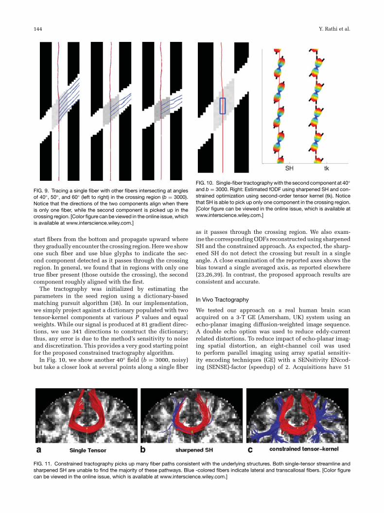
Having verified the technique’s accuracy, we now turn tothe resulting tractography. Figure 9 provides examples ofsynthetic crossing fiber fields, each at different fixed angles:40◦, 50◦, 60◦ (b = 3000, high-noise). In our experiments, we

FIG. 8. The precision of the proposed method in the presence ofvarying levels of noise. X-axis is the SNR, while the y-axis is theangular error. Blue is for b = 1000, while red is for b = 3000. [Colorfigure can be viewed in the online issue, which is available at www.interscience.wiley.com.]

144 Y. Rathi et al.

FIG. 9. Tracing a single fiber with other fibers intersecting at anglesof 40◦, 50◦, and 60◦ (left to right) in the crossing region (b = 3000).Notice that the directions of the two components align when thereis only one fiber, while the second component is picked up in thecrossing region. [Color figure can be viewed in the online issue, whichis available at www.interscience.wiley.com.]

start fibers from the bottom and propagate upward wherethey gradually encounter the crossing region. Here we showone such fiber and use blue glyphs to indicate the sec-ond component detected as it passes through the crossingregion. In general, we found that in regions with only onetrue fiber present (those outside the crossing), the secondcomponent roughly aligned with the first.

The tractography was initialized by estimating theparameters in the seed region using a dictionary-basedmatching pursuit algorithm (38). In our implementation,we simply project against a dictionary populated with twotensor-kernel components at various P values and equalweights. While our signal is produced at 81 gradient direc-tions, we use 341 directions to construct the dictionary;thus, any error is due to the method’s sensitivity to noiseand discretization. This provides a very good starting pointfor the proposed constrained tractography algorithm.

In Fig. 10, we show another 40◦ field (b = 3000, noisy)but take a closer look at several points along a single fiber

FIG. 10. Single-fiber tractography with the second component at 40◦and b = 3000. Right: Estimated fODF using sharpened SH and con-strained optimization using second-order tensor kernel (tk). Noticethat SH is able to pick up only one component in the crossing region.[Color figure can be viewed in the online issue, which is available atwww.interscience.wiley.com.]

as it passes through the crossing region. We also exam-ine the corresponding ODFs reconstructed using sharpenedSH and the constrained approach. As expected, the sharp-ened SH do not detect the crossing but result in a singleangle. A close examination of the reported axes shows thebias toward a single averaged axis, as reported elsewhere(23,26,39). In contrast, the proposed approach results areconsistent and accurate.

In Vivo Tractography

We tested our approach on a real human brain scanacquired on a 3-T GE (Amersham, UK) system using anecho-planar imaging diffusion-weighted image sequence.A double echo option was used to reduce eddy-currentrelated distortions. To reduce impact of echo-planar imag-ing spatial distortion, an eight-channel coil was usedto perform parallel imaging using array spatial sensitiv-ity encoding techniques (GE) with a SENsitivity ENcod-ing (SENSE)-factor (speedup) of 2. Acquisitions have 51

FIG. 11. Constrained tractography picks up many fiber paths consistent with the underlying structures. Both single-tensor streamline andsharpened SH are unable to find the majority of these pathways. Blue -colored fibers indicate lateral and transcallosal fibers. [Color figurecan be viewed in the online issue, which is available at www.interscience.wiley.com.]

High-order Tensor Tractography 145

FIG. 12. Close-up of upper right in Figure 11c.

gradient directions with b = 900 and eight baseline scanswith b = 0. The original GE sequence was modified toincrease spatial resolution and to further minimize imageartifacts. The following scan parameters were used: pulserepetition time 17,000 ms, echo time 78 ms, field of view24 cm, 144 × 144 encoding steps, 1.7 mm slice thickness.The scan had 85 axial slices parallel to the Anterior com-missure - Posterior commissure (AC-PC) line covering thewhole brain.

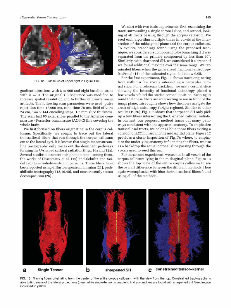
We first focused on fibers originating in the corpus cal-losum. Specifically, we sought to trace out the lateraltranscallosal fibers that run through the corpus callosumout to the lateral gyri. It is known that single-tensor stream-line tractography only traces out the dominant pathwaysforming the U-shaped callosal radiation (Figs. 10a and 12a).Several studies document this phenomenon, among them,the works of Descoteaux et al. (19) and Schultz and Sei-del (26) have side-by-side comparisons. These fibers havebeen reported using diffusion spectrum imaging (21), prob-abilistic tractography (12,19,40), and more recently tensordecomposition (26).

We start with two basic experiments: first, examining thetracts surrounding a single coronal slice, and second, look-ing at all tracts passing through the corpus callosum. Weseed each algorithm multiple times in voxels at the inter-section of the midsagittal plane and the corpus callosum.To explore branchings found using the proposed tech-nique, we considered a component to be branching if it wasseparated from the primary component by less than 40◦.Similarly, with sharpened SH, we considered it a branch ifwe found additional maxima over the same range. We ter-minated fibers when the generalized fractional anisotropy(std/rms) (14) of the estimated signal fell below 0.05.

For the first experiment, Fig. 11 shows tracts originatingfrom within a few voxels intersecting a particular coro-nal slice. For a reference backdrop, we use a coronal sliceshowing the intensity of fractional anisotropy placed afew voxels behind the seeded coronal position. Keeping inmind that these fibers are intersecting or are in front of theimage plane, this roughly shows how the fibers navigate theareas of high anisotropy (bright regions). Similar to otherresults (19,26), Fig. 10b shows that sharpened SH only pickup a few fibers intersecting the U-shaped callosal radiata.In contrast, our proposed method traces out many path-ways consistent with the apparent anatomy. To emphasizetranscallosal tracts, we color as blue those fibers exiting acorridor of ±22 mm around the midsagittal plane. Figure 12provides a closer inspection of Fig. 7c where, to empha-size the underlying anatomy influencing the fibers, we useas a backdrop the actual coronal slice passing through thevoxels used to seed this run.

For the second experiment, we seeded in all voxels of thecorpus callosum lying in the midsagittal plane. Figure 13shows the top view of the entire corpus callosum to seethe overall difference between the different methods. Hereagain we emphasize with blue the transcallosal fibers foundusing all of the methods.

FIG. 13. Tracing fibers originating from the center of the entire corpus callosum, with the view from the top. Constrained tractography isable to find many of the lateral projections (blue), while single-tensor is unable to find any and few are found with sharpened SH. Seed regionindicated in yellow.

146 Y. Rathi et al.

FIG. 14. Sagittal view with seeding in the internal capsule (yellow). While both single-tensor and sharpened SH tend to follow the dominantcorticospinal tract to the primary motor cortex, the constrained tractography method follows many more pathways.

FIG. 15. Frontal view of the cortico spinal tract in each hemisphere, with seeding done in the internal capsule (yellow).

FIG. 16. Combined view of the corpus callosum (red) and corticospinal tract (green) as obtained using constrained second-order tensorkernel. Notice that different gyri are connected to the corpus callosum and corticospinal tract.

High-order Tensor Tractography 147

FIG. 17. Figure shows crossing of the three fiber bundles in thecorona radiata. Red indicates the corpus callosum fibers, blue indi-cates direction of corticospinal tract, while yellow shows direction ofthe superior longitudinal fasciculus.

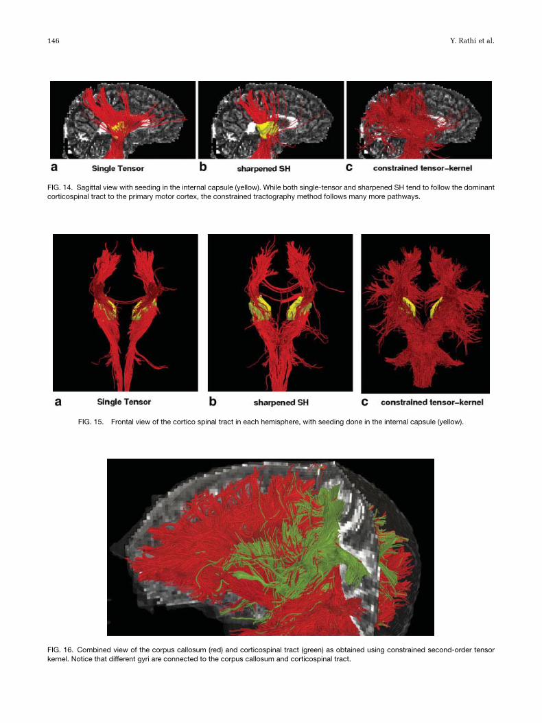
Next, we examined corticospinal tract by seeding in theinternal capsule to trace out the pathways reaching up intothe primary motor cortex at the top of the brain, as well asdown into the hippocampal regions near the brain stem.Figure 14 shows frontal views for each technique withseeding (yellow). Figure 15 shows this same result from aside view, where we can see that the constrained approachpicks up many of the corticospinal pathways, consistentwith the anatomy. Figure 16 shows a combined view ofthe corpus callosum and corticospinal tract. Notice that thetracts corresponding to each of these pathways terminatein different regions (gyri) of the brain, consistent with theanatomy. As reported elsewhere (34), single-tensor tractog-raphy only follows the dominant corticospinal tract to theprimary motor cortex. Similar pathways were also foundwith sharpened SH.

Next, we report results using the three-component model(Fig. 17). In this case, we seeded the midsagittal planeof the corpus callosum and traced the region known tocontain three crossing bundles, namely, the the superiorlongitudinal fasciculus, and corticospinal tract. The pro-posed method picks up these three major pathways, withred showing the corpus callosum fibers, blue the directionof the corticospinal tract, and yellow the superior longitu-dinal fasciculus. Thus, the three-component model is ableto pick up the three crossings in the in vivo data.

Note that when we use the two-component model, theregion of intersection between the transcallosal fibers, thecorticospinal tract, and the superior longitudinal fasci-culus, leads the tractography algorithm to report severalend-to-end connections that are not necessarily present,e.g., fibers originating in the left internal capsule do notpass through the corpus callosum. Many of the lateralextensions are callosal fibers that are picked up while pass-ing through this juncture. We believe that finding suchpathways is inevitable (in the absence of any a priori knowl-edge of the anatomy) due to poor model fitting and that theycould be removed during post processing, as is typicallydone.

DISCUSSION

Studies involving deterministic tractography rely on theunderlying model estimated at each voxel, as well as the

reconstructed pathways. In this work, we demonstratedthat, using a constrained estimation approach for tractogra-phy, robust estimates of much higher accuracy are obtainedthan independent estimation techniques. The proposedapproach gives significantly lower angular error (5◦) inregions with fiber crossings compared to using sharpenedSH (15−20◦), and it is able to reliably resolve crossingsdown to 25−20◦ compared to SH, which reaches only downto 50−60◦. In vivo results on the corpus callosum and corti-cospinal tract demonstrate the ability of the tensor kernel ina constrained mixture model framework to find fiber tractsthat are not traced using either the single tensor model orthe sharpened SH approach but are nevertheless present.

Future work involves incorporating prior knowledgeduring tractography to avoid tracts reaching in areas thatare not anatomically connected but are picked up due topartial voluming of the data. Further, we would extend thismodel to a mixture of three components to analyze in vivodata at b = 3000 or higher b-values where fiber crossingsare better detected. In Eq. 6, we assumed the noise model tobe gaussian, and future work involves using a Rician noisemodel for better estimation.

REFERENCES

1. Basser PJ, Mattiello J, LeBihan D. MR diffusion tensor spectroscopy andimaging. Biophys J 1994;66:259–267.

2. Behrens T, Woolrich M, Jenkinson M, Johansen-Berg H, Nunes R, ClareS, Matthews P, Brady J, Smith S. Characterization and propagationof uncertainty in diffusion-weighted MR imaging. Magn Reson Med2003;50:1077–1088.

3. Alexander D, Barker G, Arridge S. Detection and modeling of non-Gaussian apparent diffusion coefficient profiles in human brain data.Magn Reson Med 2002;48:331–340.

4. Frank L. Characterization of anisotropy in high angular resolutiondiffusion-weighted MRI. Magn Reson Med 2002;47:1083–1099.

5. Alexander A, Hasan K, Tsuruda J, Parker D. Analysis of partial volumeeffects in diffusion-tensor MRI. Magn Reson Med 2001;45:770–780.

6. Tuch D, Reese T, Wiegella M, Makris N, Belliveau J, Wedeen V. Highangular resolution diffusion imaging reveals intravoxel white matterfiber heterogeneity. Magn Reson Med 2002;48:577–582.

7. Kreher B, Schneider J, Mader I, Martin E, Hennig J, Il’yasov K. Multiten-sor approach for analysis and tracking of complex fiber configurations.Magn Reson Med 2005;54:1216–1225.

8. Friman O, Farnebäck G, Westin C-F. A Bayesian approach for stochasticwhite matter tractography. IEEE Trans Med Imaging 2006;25:965–978.

9. Basser PJ, Pajevic S. Spectral decomposition of a 4th-order covari-ance tensor: applications to diffusion tensor MRI. Signal Processing2007;87:220–236.

10. Barmpoutis A, Hwang MS, Howland D, Forder J, Vemuri B. Regular-ized positive-definite fourth order tensor field estimation from DW-MRI.Neuroimage 2009;1:153–162.

11. McGraw T, Vemuri B, Yezierski B, Mareci T. Von Mises-Fisher mixturemodel of the diffusion ODF. In: Int. Symp. on Biomedical Imaging, 2006.p 65–68.

12. Kaden E, Anwander A, Knsche T. Parametric spherical deconvolu-tion: inferring anatomical connectivity using diffusion MR imaging.Neuroimage 2007;37:477–488.

13. Rathi Y, Michailovich O, Shenton M, Bouix S. Directional functions fororientation distribution estimation. Med Image Anal 2009;13:432–444.

14. Tuch D. Q-ball imaging. Magn Reson Med 2004;52:1358–1372.15. Anderson A. Measurement of fiber orientation distributions using high

angular resolution diffusion imaging. Magn Reson Med 2005;54:1194–1206.

16. Hess C, Mukherjee P, Han E, Xu D, Vigneron D. Q-ball reconstruction ofmultimodal fiber orientations using the spherical harmonic basis. MagnReson Med 2006;56:104–117.

17. Descoteaux M, Angelino E, Fitzgibbons S, Deriche R. Regularized, fast,and robust analytical Q-ball imaging. Magn Reson Med 2007;58:497–510.

148 Y. Rathi et al.

18. Alexander D. Multiple-fiber reconstruction algorithms for diffusionMRI. Ann Acad Sci 2005;1064:113–133.

19. Descoteaux M, Deriche R, Anwander A, Deterministic and probabilisticq-ball tractography: from diffusion to sharp fiber distributions. In: Tech.Rep 6273, INRIA Sophia Antipolis, 2007.

20. Basser P, Pajevic S, Pierpaoli C, Duda J, Aldroubi A. In vivofiber tractography using DT-MRI data. Magn Reson Med 2000;44:625–632.

21. Hagmann P, Reese T, Tseng W-Y, Meuli R, Thiran J-P, Wedeen VJ. Diffu-sion spectrum imaging tractography in complex cerebral white matter:an investigation of the centrum semiovale. In: Int. Symp. on MagneticResonance in Medicine, 2004. p 623.

22. Zhang F, Goodlett C, Hancock E, Gerig G. Probabilistic fiber trackingusing particle filtering. In: MICCAI. 2007. p 144–152.

23. Zhan W, Yang Y. How accurately can the diffusion profiles indicate mul-tiple fiber orientations? A study on general fiber crossings in diffusionMRI. J Magn Reson 2006;183:193–202.

24. Seunarine K, Cook P, Hall M, Embleton K, Parker G, Alexander D.Exploiting peak anisotropy for tracking through complex structures. In:MMBIA, 2007. p 1–8.

25. Bloy L, Verma R. On computing the underlying fiber directions fromthe diffusion orientation distribution function. In: MICCAI, 2008.p 1–8.

26. Schultz T, Seidel H. Estimating crossing fibers: a tensor decom-position approach. IEEE Trans Vis Comput Graph 2008;14:1635–1642.

27. Ramirez-Manzanares A, Cook P, Gee J. A comparison of methods forrecovering intra-voxel white matter fiber architecture from clinicaldiffusion imaging scans. In: MICCAI, 2008. p 305–312.

28. Jian B, Vemuri B. A unified computational framework for deconvolutionto reconstruct multiple fibers from diffusion weighted MRI. IEEE TransMed Imaging 2007;26:1464–1471.

29. Jansons K, Alexander D. Persistent angular structure: new insights fromdiffusion MRI data. Inverse Problems 2003;19:1031–1046.

30. Tournier J-D, Calamante F, Gadian D, Connelly A. Direct estimation ofthe fiber orientation density function from diffusion-weighted MRI datausing spherical deconvolution. Neuroimage 2004;23:1176–1185.

31. Kumar R, Barmpoutis A, Vemuri BC, Carney PR, Mareci TH. Multi-fiberreconstruction from DW-MRI using a continuous mixture of von Mises-Fisher distributions. In: MMBIA, 2008. p 1–8.

32. Tournier J-D, Yeh C, Calamante F, Cho H, Connelly A, Lin P. Resolv-ing crossing fibres using constrained spherical deconvolution: vali-dation using diffusion-weighted imaging phantom data. Neuroimage2008;41:617–625.

33. Basser P, Pajevic S. A normal distribution for tensor-valued random vari-ables: applications to diffusion tensor MRI. IEEE Trans Med Imaging2003;22:785–794.

34. Behrens T, Johansen-Berg H, Jbabdi S, Rushworth M, Woolrich M. Prob-abilistic diffusion tractography with multiple fibre orientations: whatcan we gain? Neuroimage 2007;34:144–155.

35. Fillard VAP, Pennec X, Ayache N. Clinical DT-MRI estimation, smooth-ing and fiber tracking with log-euclidean metrics. IEEE Trans MedImaging 2007;26:1472–1482.

36. Assemlal H-E, Tschumperlé D, Brun L, A variational framework for therobust estimation of odfs from high angular resolution diffusion images,In: Tech. Rep., les cahiers du GREYC, 2007.

37. Sotiropoulos S, Bai L, Morgan P, Auer D, Constantinescu C, Tench C.A regularized two-tensor model fit to low angular resolution diffusionimages using basis directions. J Magn Reson Med 2008;28:199–209.

38. Mallat S, Zhang Z. Matching pursuits with time-frequency dictionaries.IEEE Trans Signal Process 1993;41:3397–2415.

39. Tournier J-D, Calamante F, Connelly A. Robust determination of the fibreorientation distribution in diffusion MRI: non-negativity constrainedsuper-resolved spherical deconvolution. Neuroimage 2007;35:1459–1472.

40. Anwander A, Descoteaux M, Deriche R. Probabilistic Q-Ball tractog-raphy solves crossings of the callosal fibers. in: Human Brain Mapp,volume 1, 2007. p 342.