SPE 145684

Production Characteristics of the Bakken Shale Oil Tan Tran, Pahala Sinurat, and R.A Wattenbarger, SPE, Texas A&M University

Copyright 2011, Society of Petroleum Engineers This paper was prepared for presentation at the SPE Annual Technical Conference and Exhibition held in Denver, Colorado, USA, 30 October–2 November 2011. This paper was selected for presentation by an SPE program committee following review of information contained in an abstract submitted by the author(s). Contents of the paper have not been reviewed by the Society of Petroleum Engineers and are subject to correction by the author(s). The material does not necessarily reflect any position of the Society of Petroleum Engineers, its officers, or members. Electronic reproduction, distribution, or storage of any part of this paper without the written consent of the Society of Petroleum Engineers is prohibited. Permission to reproduce in print is restricted to an abstract of not more than 300 words; illustrations may not be copied. The abstract must contain conspicuous acknowledgment of SPE copyright.

Abstract

There are three main types of well production trends in the Bakken formation. Each decline curve characteristic of these production trends has an important meaning to the production trends of the Bakken Shale play especially type I and type II production trends. In the total of 146 well histories, there are 51 % of wells in Type I production trend. This high percentage of Type I production trend is showing the true characteristic of the Bakken Shale reservoir, which will be discussed later in this paper. Type I production trend has the reservoir pressure drops below bubble point pressure and gas releasing out of the solution. This can be seen on the GOR curve vs. time plot. The cause of reservoir drop below bubble point has been analyzed, and the production of oil in this behavior has driving force from the solution gas. In additional, two linear flow regimes have been observed by looking at the log-log plot of rate against time plot of type I well.

In a type II production trend, production is primary from the matrix. Reservoir pressure is higher than the bubble point pressure during the producing time and oil flows as a single phase throughout the production period of the well. GOR curve is almost constant during the production period. A single linear flow behavior is observed in Bakken Shale play of type II wells. This behavior is characterized by a half-slope on the log-log plot of the oil rate versus time plot.

A type III production trend typically has scattering production data from wells with a different type of trends. It is difficult to study this type of behavior because of scattering data and it will lead to uncorrected interpretation for the analysis.

Calculation procedures are given for OIIP estimation, and the area of matrix drainage between fractures, Acm.

Introduction Area of interest covers nine different counties from the Bakken Shale formation. Most counties are from North Dakota state with twenty years of the production histories. These well histories are producing from upper and middle member of the Bakken formation. The production trends from these production histories are inconsistent. Some production trends seem to have better cumulative oil than others. So understanding the production characteristics of the Bakken Shale play is key to success for the operation companies in the area.

This paper describes the production characteristics over the Bakken Shale Oil play, one of the largest shale plays in the United State. OOIP and the area of matrix drainage between the fractures estimations are also given.

Bakken Shale Geology

The Bakken formation is located in the Williston Basin. It was first discovered in 1953 (Breit et al. 1992) when the Antelope Field was discovered. The Bakken Shale play is a shale oil play and has an area of 225,000 squares miles (Price 1986). It is shared by Canada and the United States and is located in North Dakota, South Dakota, Montana, and Saskatchewan.

2 SPE 145684

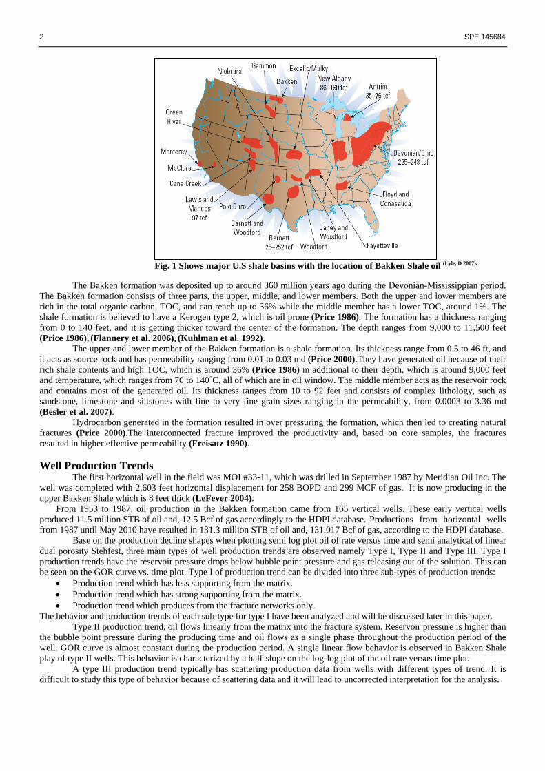
Fig. 1 Shows major U.S shale basins with the location of Bakken Shale oil (Lyle, D 2007).

The Bakken formation was deposited up to around 360 million years ago during the Devonian-Mississippian period. The Bakken formation consists of three parts, the upper, middle, and lower members. Both the upper and lower members are rich in the total organic carbon, TOC, and can reach up to 36% while the middle member has a lower TOC, around 1%. The shale formation is believed to have a Kerogen type 2, which is oil prone (Price 1986). The formation has a thickness ranging from 0 to 140 feet, and it is getting thicker toward the center of the formation. The depth ranges from 9,000 to 11,500 feet (Price 1986), (Flannery et al. 2006), (Kuhlman et al. 1992).

The upper and lower member of the Bakken formation is a shale formation. Its thickness range from 0.5 to 46 ft, and it acts as source rock and has permeability ranging from 0.01 to 0.03 md (Price 2000).They have generated oil because of their rich shale contents and high TOC, which is around 36% (Price 1986) in additional to their depth, which is around 9,000 feet and temperature, which ranges from 70 to 140˚C, all of which are in oil window. The middle member acts as the reservoir rock and contains most of the generated oil. Its thickness ranges from 10 to 92 feet and consists of complex lithology, such as sandstone, limestone and siltstones with fine to very fine grain sizes ranging in the permeability, from 0.0003 to 3.36 md (Besler et al. 2007).

Hydrocarbon generated in the formation resulted in over pressuring the formation, which then led to creating natural fractures (Price 2000).The interconnected fracture improved the productivity and, based on core samples, the fractures resulted in higher effective permeability (Freisatz 1990).

Well Production Trends

The first horizontal well in the field was MOI #33-11, which was drilled in September 1987 by Meridian Oil Inc. The well was completed with 2,603 feet horizontal displacement for 258 BOPD and 299 MCF of gas. It is now producing in the upper Bakken Shale which is 8 feet thick (LeFever 2004).

From 1953 to 1987, oil production in the Bakken formation came from 165 vertical wells. These early vertical wells produced 11.5 million STB of oil and, 12.5 Bcf of gas accordingly to the HDPI database. Productions from horizontal wells from 1987 until May 2010 have resulted in 131.3 million STB of oil and, 131.017 Bcf of gas, according to the HDPI database. Base on the production decline shapes when plotting semi log plot oil of rate versus time and semi analytical of linear dual porosity Stehfest, three main types of well production trends are observed namely Type I, Type II and Type III. Type I production trends have the reservoir pressure drops below bubble point pressure and gas releasing out of the solution. This can be seen on the GOR curve vs. time plot. Type I of production trend can be divided into three sub-types of production trends:

• Production trend which has less supporting from the matrix. • Production trend which has strong supporting from the matrix. • Production trend which produces from the fracture networks only.

The behavior and production trends of each sub-type for type I have been analyzed and will be discussed later in this paper. Type II production trend, oil flows linearly from the matrix into the fracture system. Reservoir pressure is higher than

the bubble point pressure during the producing time and oil flows as a single phase throughout the production period of the well. GOR curve is almost constant during the production period. A single linear flow behavior is observed in Bakken Shale play of type II wells. This behavior is characterized by a half-slope on the log-log plot of the oil rate versus time plot.

A type III production trend typically has scattering production data from wells with different types of trend. It is difficult to study this type of behavior because of scattering data and it will lead to uncorrected interpretation for the analysis.

SPE 145684 3

Production Trend Types

1. Type I

o Production trend which has less supporting from the matrix: This type of production trend shows a fast decline initially then changes to a steady and slow decline as shown in Fig. 2

Fig. 2 Shows production trend which has less supporting from the matrix.

o Production trend which has strong supporting from the matrix: This type of production trend shows a short rapid decline initially then changes to a steady and slow declines as shown in Fig. 3

Fig. 3 Shows production trend which has strong supporting from the matrix.

4 SPE 145684

o Production trend which produces from the fracture networks only: This type of production trend shows a long rapid decline but does not change the slope of the curve later as shown in Fig. 4

Fig. 4 Shows production trend which produces from fracture system only.

2. Type II: production trend which produces from the matrix only. This type of production trend shows only oil production for most of the well life.

Fig. 5 Shows production trend type II.

SPE 145684 5

Reservoir performance under these production trends

o Reservoir performance for production trend which has less supporting from the matrix: In order to describe the reservoir performance, two plots including semi log plot of rate vs. time and log-log plot of rate vs. time are given as Fig. 6.

0.0001

0.001

0.01

0.1

1

10

100

1000

10000

0 2,000 4,000 6,000 8,000

Rate, BPD

,Mscf/Day

Time, Days

Well 1

Oil Gas Water

0.0001

0.001

0.01

0.1

1

10

100

1000

10000

30 300 3,000 30,000

Rate, B

PD,M

scf/Day

Time, Days

Well 1

Oil Gas Water

3½ slope line

Matrix Supporting

1

32Fracture

dominated flow

½ slope line

2 Matrix Supporting

1

Fig. 6 Reservoir performance for production trend which has less supporting from the matrix.

The reservoir performance for this type of production trend can be described as:

o Initially single phase oil flows linearly from the fracture networks into the well. Reservoir pressure at this point is still above the bubble point pressure but continue to drop fast. These behaviors can be seen on the semi log straight line as the period one and on the log-log as the first ½ slope straight line. Notice that the time for this period on the two plots, is corresponding. It is about 15 months, 500 days.

o Oil will continue to flow inside the fracture network until the pressure drop reaches the end of fracture

network; transient period is end inside the fracture network. At this time the reservoir pressure is dropping below the bubble point pressure and gas starts releasing out of solution. Oil still flows from fracture network into the well but it is not linear flow. This can be seen on the log-log plot when the oil production curve is deviated from ½ slope curve, indicating pressure drop reaches the end of fracture network boundary. Gas releases out of solution, and it can be seen as gas production curve on the semi log plot. Oil production rate continue to drop fast as seen by oil production curve on the semi log plot of oil rate decline curve, periods two.

o The matrix starts to drain into the fracture network, resulting in the decreasing of gas production. This behavior can be seen from the short decreasing of the gas production curve on the semi log plot. When the supporting from the matrix is strong enough, both the oil and gas production rate will be stabilized. This behavior can be seen at the period three on the semi log and log-log plot. Also second ½ slope line appears again on the log-log plot. This stabilized period also can be seen on the GOR as shown in Fig. 7 below.

6 SPE 145684

0.0001

0.001

0.01

0.1

1

10

100

1000

10000

0 2,000 4,000 6,000 8,000

Rate, B

PD,M

scf/Day

Time, Days

Well 1

Oil Gas Water

1

10

100

1,000

10,000

100,000

30 300 3,000 30,000

GOR, M

scf/Bb

l

Time, Days

Well 1

GOR

The flattening curves is showing the stabilized condition due to pressure supporting from the matrix

The flattening curves is showing the stabilized condition due to pressure supporting from the matrix

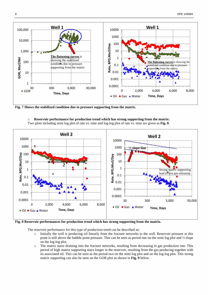
Fig. 7 Shows the stabilized condition due to pressure supporting from the matrix.

o Reservoir performance for production trend which has strong supporting from the matrix: Two plots including semi log plot of rate vs. time and log-log plot of rate vs. time are given as Fig. 8.

0.0001

0.001

0.01

0.1

1

10

100

1000

10000

0 2,000 4,000 6,000 8,000

Rate, B

PD,M

scf/Day

Time, Days

Well 2

Oil Gas Water

0.0001

0.001

0.01

0.1

1

10

100

1000

10000

30 300 3,000 30,000

Rate, B

PD,M

scf/Day

Time, Days

Well 2

Oil Gas Water

½ slope line 1

2Strong matrix supporting lead to less gas releasing

Fig. 8 Reservoir performances for production trend which has strong supporting from the matrix.

The reservoir performance for this type of production trend can be described as: o Initially the well is producing oil linearly from the fracture networks to the well. Reservoir pressure at this

point is still above the bubble point pressure. This can be seen as period one on the semi log plot and ½ slope on the log-log plot.

o The matrix starts draining into the fracture networks, resulting from decreasing in gas production rate. This period of high matrix supporting stays longer in the reservoir, resulting from the gas producing together with its associated oil. This can be seen as the period two on the semi log plot and on the log-log plot. This strong matrix supporting can also be seen on the GOR plot as shown in Fig. 9 below.

SPE 145684 7

o The cause of having strong matrix supporting for this Type is of the higher permeability inside the matrix outside of the fracture network compare to the previous one. This higher permeability is result of possibly more natural fractures around the area.

1

10

100

1,000

10,000

30 300 3,000 30,000

GOR, M

scf/Bb

l

Time, Days

Well 2

GOR

0.0001

0.001

0.01

0.1

1

10

100

1000

10000

0 2,000 4,000 6,000 8,000Rate, B

PD,M

scf/Day

Time, Days

Well 2

Oil Gas Water

Strong matrix supporting lead to less gas releasing

Strong matrix supporting lead to GOR close to initial GOR.

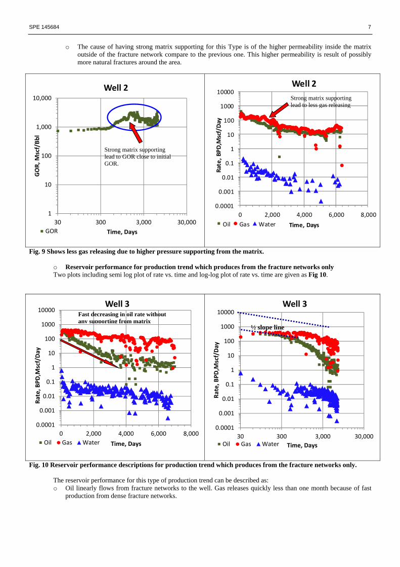
Fig. 9 Shows less gas releasing due to higher pressure supporting from the matrix.

o Reservoir performance for production trend which produces from the fracture networks only Two plots including semi log plot of rate vs. time and log-log plot of rate vs. time are given as Fig 10.

0.0001

0.001

0.01

0.1

1

10

100

1000

10000

0 2,000 4,000 6,000 8,000

Rate, B

PD,M

scf/Day

Time, Days

Well 3

Oil Gas Water

0.0001

0.001

0.01

0.1

1

10

100

1000

10000

30 300 3,000 30,000

Rate, B

PD,M

scf/Day

Time, Days

Well 3

Oil Gas Water

½ slope line

Fast decreasing in oil rate without any supporting from matrix

Fig. 10 Reservoir performance descriptions for production trend which produces from the fracture networks only.

The reservoir performance for this type of production trend can be described as: o Oil linearly flows from fracture networks to the well. Gas releases quickly less than one month because of fast

production from dense fracture networks.

8 SPE 145684

o Oil continues to flow inside the fracture networks to the well until the pressure drop reaches the end of fracture inside the fracture network. This can be seen on the log-log plot when the oil rate deviated from ½ slope around 5 months, 150 days.

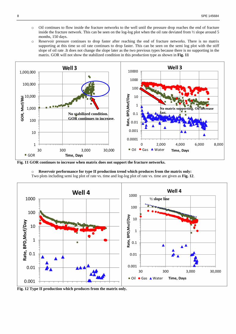
o Reservoir pressure continues to drop faster after reaching the end of fracture networks. There is no matrix supporting at this time so oil rate continues to drop faster. This can be seen on the semi log plot with the stiff slope of oil rate .It does not change the slope later as the two previous types because there is no supporting in the matrix. GOR will not show the stabilized condition in this production type as shown in Fig. 11

1

10

100

1,000

10,000

100,000

1,000,000

GOR, Mscf/Bbl

Well 3

30 300 3,000 30,000Time, DaysGOR

0.0001

0.001

0.01

0.1

1

10

100

1000

10000

0 2,000 4,000 6,000 8,000

Rate, B

PD,M

scf/Day

Time, Days

Well 3

Oil Gas Water

No matrix supporting. Oil decrease fast. No stabilized condition.

GOR continues to increase.

Fig. 11 GOR continues to increase when matrix does not support the fracture networks.

o Reservoir performance for type II production trend which produces from the matrix only: Two plots including semi log plot of rate vs. time and log-log plot of rate vs. time are given as Fig. 12.

0.001

0.01

0.1

1

10

100

1000

30 300 3,000 30,000

Rate, B

PD,M

scf/Day

Well 4

0.001

0.01

0.1

1

10

100

1000

Rate, B

PD,M

scf/Day

Well 4

Time, DaysOil Gas Water

½ slope line

Fig. 12 Type II production which produces from the matrix only.

SPE 145684 9

The reservoir performance for this type of production trend can be described as: o Type II production shows a single exponential decline on semi log plot. Gas does not release, and there is short

period of increasing gas at the end but this is scattering field data collection or some workovers which try to increase production. Oil and gas are produced together for the entire of production life. The drive performance for the type II is oil expansion drive and producing from low permeability matrix only. This can be seen clearly on the log-log plot. GOR of this well shows constant for the entire of production life as shown in Fig. 13.

1

10

100

1,000

10,000GOR, M

scf/Bb

lWell 4

30 300 3,000Time, DaysGOR

Fig. 13 GOR of type II production.

OOIP Estimation and Area of matrix drainage, Acm This section will describe the procedures for calculation OOIP, area of matrix drainage, Acm .Linear dual porosity “transient slab model” El-Banbi (1998) is applied for the calculation. In this model, Bello (2009) found that there are five flow regions that horizontal well may have throughout the well production life. In that five flow regions, Region 4 is the transient flow from the matrix to the fractures.

In order to apply the linear dual porosity slab model we need to have the hydraulic fracture data including fracture spacing and number of fractures. Wells from the analysis above only have the production data and so we could not apply the calculation on those wells. Wells that available for the calculation have only three years of production histories as show in the Fig. 14 is one of the examples.

10 SPE 145684

½ slope line

Fig. 14 Semi-log and log-log plot of oil, gas production vs. time. There only one linear flow for the well 6 above and we could assume well 6 produce from the matrix only, Type II, and has reached the boundary dominate flow. We now apply the model 1 Al-Ahmadi et al. (2010) as shown in Fig. 15 below

xe = Drainage area length

Horizontal Well

2ye = Hydraulic fracture length

Hydraulic Fracture Spacing L

Fig. 15 Dual porosity slab matrix, model 1. In this model the equation for calculation OOIP, Acm, and fracture half length, ye are given as: El-Banbi (1998). ………………………………………………………………………………….. (1)

4 )St

OOIP hs −1(91.19mct

we=

…………………………………………………………………………………… (2)

4

1)(

k 1.125mc

BAt

cmm φμμ

=

)(1591.0

t

ehsme c

yφμ

=tk ………………………………………………………………………………………… (3)

SPE 145684 11

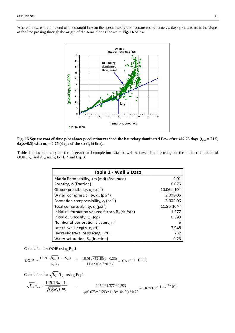
Where the tehs is the time end of the straight line on the specialized plot of square root of time vs. days plot, and m4 is the slope of the line passing through the origin of the same plot as shown in Fig. 16 below

Boundary dominated flow period

tehs

Fig. 16 Square root of time plot shows production reached the boundary dominated flow after 462.25 days (tehs = 21.5, days^0.5) with m4 = 0.75 (slope of the straight line). Table 1 is the summary for the reservoir and completion data for well 6, these data are using for the initial calculation of OOIP, ye, and Acm using Eq 1, 2 and Eq. 3.

Table 1 ‐Well 6 Data Matrix Permeability, km (md) (Assumed)       0.01 Porosity, φ (fraction)          0.075 Oil compressibility, co (psi

‐1)          10.06 x 10‐6 Water  compressibility, cw (psi

‐1)       3.00E‐06 Formation compressibility, cf (psi

‐1)       3.00E‐06 Total compressibility, ct (psi

‐1)          11.8 x 10^‐6 Initial oil formation volume factor, Boi(rbl/stb)     1.377 Initial oil viscosity, µoi (cp)          0.593 Number of perforation clusters, nf       5 Lateral well length, xe (ft)          2,948 Hydraulic fracture spacing, L(ft)       737 Water saturation, Sw (fraction)          0.23 

Calculation for OOIP using Eq.1

= 4

66 ^1037

75.0*^10*8.11)23.01(25.46291.19

×=−

− (bbls)

)1(1c

StOOIP whs −9.19

mt

e=

Calculation for cmm Ak using Eq.2

= 4

1)(

k 1.125mc

BAt

cmm φμμ

= 5

6^1087.1

75.0*)^10*8.11*593.0*075.0(

593.0*377.1*1.125×=

−

(md 0.5 ft2)

12 SPE 145684

With km = 0.01 md, then Acm is estimated as:

Acm = 61087.101.0

187000×= (ft2)

Calculation for hydraulic fracture half length using Eq.3

)(1591.0

t

ehsme c

tkyφμ

= = 7.470^10*8.11*593.0*075.0

25.462*01.01591.0 6 =− (ft)

With these reservoir parameter results, we then use the numerical simulation Gassim to history match with the field production, to obtain a reasonable accuracy for the reservoir properties. The result plots for the simulation run compare to field production are shown in Fig. 17 below.

Fig. 17 Show simulation result compares to field production data.

Obviously, we see on the Fig. 17 there are disagreements between the analytical calculation and the numerical simulation.This disagreement is because of the uncertainty in the reservoir properties such as matrix permeability and porosity. In order to obtain a better match, we perform few more simulation run with changing matrix permeability and porosity. A better match was obtained as shown in Fig.18 below

SPE 145684 13

Fig. 18 Show a better match of field production data compare to numerical simulation.

Table 2 summaries the final result for well 6

Table 2 ‐ Well 6  final results Matrix Permeability, km (md)         0.0113 Porosity, φ (fraction)          0.04 

Area of matrix drainage, Acm, (ft2)        2.41*10^6 

OOIP (bbls)        28*10^6 

Hydraulic fracture half length, (ft)        685  Conclusions

• Type I production trend associates with the reservoir pressure drops below bubble point pressure. This type of production is produced from large fracture system.

• Type II production does not have fracture dominated flow only matrix flow, resulting in lower cumulative oil recovery than Type I production.

• Calculation procedures for OOIP, fracture half length, and Area of matrix drainage, Acm are given by applying analytical solutions for dual porosity slab model and numerical simulation together to obtain reservoir properties.

• Using a multi-phase simulation to forecast well future performances base on the obtained results is a recommendation.

Nomenclature km = Matrix permeability, md Acm = Area of matrix drainage into the fracture system, ft2 OOIP = Original oil in place, bbls Boi = Initial oil formation volume factor, rbl/stb µoi = Initial oil viscosity, cp tehs = Time end of the straight line on the specialized plot of square root of time, days xe = Lateral well length, ft m4 = Slope of the straight line passing through the origin of the square root of time plot L = Hydraulic fracture spacing, ft ye = Hydraulic fracture half-length, ft µoi = Initial oil viscosity, cp Sw = Water saturation, fraction φ   =     Porosity, fraction   

14 SPE 145684

Acknowledgments The authors wish to acknowledgment financial support of the Reservoir Modeling Consortium at Texas A&M University. Also sincerely, the authors wish to acknowledgment the numerous helpful suggestions made by colleagues during the works. References Al-Ahmadi, H.A, Almarzooq, A.M., and Wattenbarger, R.A. 2010. Application of Linear Flow Analysis to Shale Gas Wells- Field Cases. Paper SPE 130370 presented at the SPE Unconventional Gas, Pittsburgh, PA, 23-25 February. Bello, R.O.2009. Rate Transient Analysis in Shale Gas Reservoirs with Transient Linear Behavior. Ph.D. dissertation, College Station; Texas A&M University. Besler, M.R., Steele, J.W., Egan, T., and Wagner, J. 2007. Improving Well Productivity and Profitability in the Bakken: A Summary of Our Experiences Drilling, Stimulating, and Operating Horizontal Wells. Paper SPE 110679 presented at the SPE Annual Technical Conference and Exhibition, Anaheim, CA, 11-14 November.

Breit, V.S, Stright Jr., D.H., Dozzo, J.A. 1992. Reservoir Characterization of the Bakken Shale from Modeling of Horizontal Well Production Interference Data. Paper SPE 24320 presented at the SPE Annual Rocky Mountain Regional Meeting, Casper,WY,18-21May. El-Banbi, A.H. 1998. Analysis of Tight Gas Wells. Ph.D. dissertation, College Station; Texas A&M University. Flannery, J., and Kraus, J. 2006. Integrated Analysis of the Bakken Petroleum System U.S. Williston Basin 2006 AAPG Bulletin. http://www.searchanddiscovery.net/documents/2006/06035flannery/index.htm

Freisatz W.B. 1990. Fracture-enhanced Porosity and Permeability Trends in Bakken Formation, Williston Basin, Western North Dakota. American Association of Petroleum Geologists, 74: 870-1324. Kuhlman. R.D., Perez, J.I., and Claiborne, E.B. 1992. Microfracture Stress Tests, Anelastic Strain Recovery, and Differential Strain Analysis Assist in Bakken Shale Horizontal Drilling Program. Paper SPE 24379 presented at the SPE Annual Rocky Mountain Regional Meeting. Casper, WY, 18-21 May. LeFever, J. A. 2004. Evolution of Oil Production in the Bakken Formation, North Dakota Geological Survey paper, presented at the 2004 Petroleum Council. https://www.dmr.nd.gov/ndgs/bakken/bakken.asp Lyle, D. 2007.Shale Gas Plays Expand, 1-March, Retrieved 7-August 2010 from http://www.epmag.com/archives/features/304.htm Price, L.C. 1986. Organic Metamorphism in the Lower Mississippian-upper Devonian Bakken Shale. Journal of Petroleum Geology. 9: 313-342. Price, L.C. 2000. Origins and Characteristics of the Basin-Centered Continuous Reservoir Unconventional Oil-Resource Base of the Bakken Source System, Williston Basin. http://www.undeerc.org/Price/