ten years of rail roughness control in the netherlands ... et...ten years of rail roughness control...

Ten years of rail roughness control in the Netherlands – Lessons learned

Wout Schwanen, Ard Kuijpers M+P consulting engineers, Vught, The Netherlands

Job Torbijn Infraspeed Maintenance bv, Dordrecht, The Netherlands

Summary

Reducing the rail roughness is a well-known and accepted noise mitigation measure for railways. When the rail roughness is reduced, the excitation of rolling noise is effectively reduced at the source.

Rail roughness is not constant over time: after reducing the rail roughness by grinding, the roughness and consequently the rolling noise emission will increase again. This means that the factor time has to be taken into account both in noise impact studies and in the maintenance regime. In practice, the time development is taken into account by using the time-averaged roughness level in noise impact studies and by monitoring the rail roughness level during maintenance to obtain this average. Monitoring is an essential part of the noise mitigation measure, because it is needed to demonstrate to the authorities that a certain average noise reduction is achieved and to know when the rail needs to be grinded again to assure that a desired average roughness level is obtained.

The combination of rail grinding and monitoring the rail roughness is used on the high speed line in the Netherlands. Infraspeed Maintenance bv has incorporated rail roughness control in their asset management strategy now. They have to demonstrate to the authorities that the track stays within certain noise emission limits and they do that by monitoring the rail roughness on a regular base and grinding the rail when needed. Thus a certain average noise emission reduction is guaranteed.

PACS no. 43.50.+y

1. Introduction

The high speed line in the Netherlands, HSL-Zuid, is constructed with Rheda track, a concrete ballastless track system with sleepers embedded in a concrete slab. When a train drives over Rheda track it produces more rolling noise than driving over the Dutch reference track: UIC54 ballasted track with concrete sleepers. The reason for this is the lower track decay rate of the Rheda rail system compared to ballasted track with concrete sleepers.The decision to use concrete slab track was made after the route was set in stone, meaning the extra noise was not considered in the planning phase. The Dutch government decided that it was only allowed to use the Rheda track if the extra noise pollution could be eliminated without increasing the height of the scheduled noise barriers. In the design phase of the HSL-Zuid, suitable noise mitigation measures were considered to

eliminate the extra noise emission of Rheda track. Noise reduction was not the only factor that was taken into account. A RAMS analysis was made to weigh all relevant aspects of the possible noise mitigation measures. Acoustic grinding scored best for almost all factors and turned out to be the best solution for the whole track. However, acoustic grinding was never used before on such a scale in the Netherlands. Hence, there was no accepted methodology for monitoring and assessing the quality of the track after grinding available. So the first step was to develop such a methodology [1]. The combination of monitoring the rail roughness and condition-based grinding is in use for ten years now. The idea started on the drawing board but is now incorporated in the asset management strategy of Infraspeed Maintenance bv. It is the first time in the Netherlands that rail roughness control has been applied successfully on such a large scale.

1

This paper gives an overview of how rail roughness control is applied on the HSL-Zuid. It summarizes the lessons learned in the ten years that this maintenance strategy has been used on the high speed line. It explains which challenges, technically as well as procedurally, were overcome to bring the idea from the drawing board into practice.

2. Rail roughness control as a noise mitigation measure

Rail grinding is a noise mitigation measure that reduces the rolling noise of trains at the source. By reducing the rail roughness, the combined roughness of the wheel and the rail is reduced. This decreases the excitation of wheel and rail vibrations leading to a lower sound radiation into the surroundings. Lowering the rail roughness is only effective when the wheel roughness is sufficiently low. If the wheel roughness is too high it dominates the combined roughness and lowering the rail roughness has no effect at all.

3. Monitoring rail roughness

Rail roughness is not constant over time. So there is a need for measurement and monitoring methods to assess the actual noise reduction and to monitor the development of the rail roughness. The results of the monitoring are used to schedule grinding maintenance to achieve a certain average noise reduction over a period of time. The monitoring method on the HSL-Zuid uses a combination of direct and indirect rail roughness measurements with ARRoW [2]. The combination of measurement techniques is a compromise between accuracy and practicality.

3.1. Direct measurement Direct measurement of the rail roughness would be a suitable way to monitor the rail roughness. It yields very accurate results that can be translatedinto a noise reduction. However, application of this method on the HSL-Zuid is not practicable because a lot of measurements would be needed to get a good impression of the rail roughness of the whole track. Furthermore, the track has to be out of service to perform direct measurements and the procedure is quiet labor intensive.

3.2. Indirect measurement To overcome the drawbacks of direct measurements one can use indirect rail roughness measurements to monitor the rail roughness of the whole track. The indirect rail roughness method consists of rolling noise measurements in close proximity of the wheel-rail contact area. For a given wheel roughness and track system, there is a direct relationship between the variation in sound levels and the variation of rail roughness. Thus by measuring the sound variation we know the variation in rail roughness. However, this method yields only relative results and we cannot express these results directly into absolute changes of the rolling noise emission level.

3.3. Combining the direct and indirect method It was decided to combine both methods to monitor the rail roughness of the HSL-Zuid. The relative results of the noise measurements are made absolute because the indirect results are calibrated on reference sections and hence, the relative results can be shifted to absolute results (see Figure 1). There exists a direct spectral relationship between the combined roughness of wheel and rail and the change in the noise emission

(1)

With Lp,grinding,I as the difference in noise level between ground and a reference track, Lr,veh as the wheel roughness level, Lr,tr as the rail roughness level, denoting energetic summation and i denoting the frequency band. Roughness is normally expressed as a function of wavelength, . We have to use a spectral translation to use roughness as a function of frequency, f. This translation is based upon the well-known relationship between frequency and wavelength depending on the vehicle speed f = v\ .

Figure 1. combining direct and indirect rail roughnessmeasurement results

EuroNoise 201531 May - 3 June, Maastricht

W. Schwanen et al.: Ten years of...

2

Equation (1) can be used to translate the results of the direct measurements into a change of rolling noise level for an assumed wheel and average rail network track. In the Netherlands these are available e.g. in the Dutch standard noise impact model [3] and in its successor. When using the indirect method, the rolling noise level is directly measured, but the difference in sound emission level between the ground and the average track is unknown. However, we still can use equation (1). We assume that the variation in rolling noise results only from variations in rail roughness. So we can determine the sound spectrum difference between section A and section B. Given that section A is a reference level and we know the rail roughness level at that section we can determine the rail roughness level at section B. By using multiple reference locations we can determine a reliable estimate of the rail roughness for the whole track.

4. Current monitoring practice on the HSL-Zuid

4.1. Measurement systems

4.1.1. Direct rail roughness measurement devices The direct roughness measurements have been conducted with the Müller-BBM 1200e, its successor the m|rail and the ØDS TRM02 devices. The measurements are performed and analyzed according the EN15610: 2009 standard [4]. We proved that all systems are able to deliver results accurate enough to determine the noise reduction by grinding. Figure 2 shows the results of a comparison test made on the HSL-Zuid between two devices. The resulting Cb,c-values, which are

an average over the left and the right rail, for both devices are almost identical.

4.1.2. ARRoW measurement system The indirect roughness measurements are performed with ARRoW. ARRoW was developed especially for the purpose of rail roughness monitoring on the HSL-Zuid. Since then it has also been used in various projects to assess the state of the railway track ([5], [6]). It measures rolling noise, position and speed on board of a measurement vehicle. The system consists of four removable microphones combined with a GPS receiver. The microphones are placed in close proximity of the wheel/rail interface to directly measure the rolling noise and minimize the influence of interfering reflections and other noise sources (see Figure 3). A GPS sensor is used to measure the speed and the position of the vehicle. ARRoW measures the sound at multiple wheels on the same bogie. The microphones are placed on the outside of the wheel. This has various advantages: (i) we can easily mount and dismount the microphones. (ii) It enables us to distinguish between the results of the left and the right rail and (iii) it introduces an extra redundancy in the measurement chain. When one microphone breaks down during the measurement we can still use the data of the other microphones. However, the current microphone positions are more sensitive to reflections from sidewalls than a system at which the microphones are placed on the inner side of the wheels (see section 6.2).

4.2. Data acquisition and analysis During an ARRoW-measurement the sound levels are recorded along with the GPS-position and the vehicle speed. Hence, we know where we are and

Figure 3. ARRoW system on the BAM measurement vehicle

Figure 2 Comparison of the resulting Cb,c-value for two rail roughness measurement devices. The values shown are an average of the measurement result on the left and right rail.

-2

-1

0

1

A B C

C b,c

[dB]

measurement location

device 1device 2



3

how fast we were driving at that time. At each reference location we measured the rail roughness directly. Around the reference location we determine the average sound spectra over a certain evaluation length (e.g. 20 meters). For each location at the track we now determine the difference in sound level spectrum with each reference location. We use equation (1) to determine the rail roughness spectrum at that position. If e.g. we use five calibration locations we obtain five estimates for the rail roughness. We determine an average rail roughness spectrum over all these estimates. A further averaging over left and right side microphones and over a certain chainage section length is required as a final step. For the HSL-Zuid, the noise reduction effect due to grinding is evaluated over 1 km sections. This evaluation length and averaging process has been agreed upon with the environmental authorities. Figure 4 shows a typical result of this procedure. The green line shows the local value for the noise reduction and the black line shows the average per evaluation length of 1 km. For this particular case, the momentary noise immission correction coefficient, Cb,c is below 0 dB for the whole track which means that the track is more silent than the reference track. This average noise reduction is the actual parameter for which the noise limits are stated.

5. Environmental noise limits

The track complies with the environmental limits when the time-averaged noise immission

difference is below 0 dB. When this is the case the extra noise originating from the Rheda track is compensated for by the rail roughness. When the time-averaged Cb,c-value is above 0 dB the track does not comply and grinding is necessary. The time-averaged Cb,c-value is calculated over a defined timespan, which started when track was taken into service. The timespan stops when the track is ground. At that moment we start a new timespan to calculate the time-averaged Cb,c-value. This does complicate things considerably: acoustic grinding is only needed for that part of the track where the rail roughness is too high. This means that the time interval for averaging is different at different parts of the whole track. This means that the moment of grinding has to be remembered as part of the asset management.

6. Practical considerations

The monitoring procedure has been applied for almost ten years now. We have gained a lot of experience with the measurements and the data analysis. Below we will discuss the major findings.

6.1. Vehicle speed A reliable constant vehicle speed is of uttermost importance. The vehicle speed directly influences the rolling noise. Every deviation from the reference speed introduces a possible source of inaccuracy. Small deviations can be corrected for with a logarithmic scaling. But when the speed differs significantly from the reference speed a simple logarithmic scaling alone is not enough. We then have to take into the account that there is also a possible frequency shift (f=v\ ), which complicates the data processing. We therefore used another option to overcome this problem: we increase the number of reference sections. By assuring there are reference sections with various speeds we can do the analysis multiple times for various reference speeds. As a final step, we have to combine all the results into one, taking into the account the actual vehicle speed during the measurements. The drawback is that the number of reference sections increase and therefore the total measurement effort. So it is recommended to instruct the measurement train driver to keep the measurement speed as constant as possible.

Figure 4. A-weighted noise immission coefficient Cb,c

measured at the HSL-Zuid. The green line shows the local value, the black line indicates the average over a length of 1km. The red dots indicate the results for the Cb,c-value at the calibration locations.



4

6.2. The direct surroundings of the track The rolling noise might change due to other sources than the rail roughness alone, e.g. due to sidewalls which cause reflections of the emitted noise. We minimize this influence by measuring very close to the wheel/rail interface and thus lengthening the reflection path, but the secondary reflection is sometimes still considerable. We are still looking into ways to diminish this effect. One could think of several solutions, like using an enclosure around the wheel and microphone to reduce the reflections. Another way would be to determine the possible effect of reflections and correct the rolling noise accordingly, depending on the actual surroundings. This is a complicated process however because we need to track the surroundings. Additionally the influence of the surroundings on the sound level can depend on the measurement vehicle. So, a possible correction of the measurement sound levels should be determined for each used measurement vehicle separately. At the moment we choose to perform a rail roughness measurement if we suspect that the result of the indirect measurement is influenced by the direct surroundings.

6.3. Scheduling the direct measurements Ideally, we first would like to perform the ARRoW-measurements and then define the locations to measure the rail roughness directly. It turned out that this caused much delay and the timespan between the direct and indirect measurements would become too big. We solved this by defining a set of reference locations that are measured each time. In addition we schedule in advance an additional moment to measure //the rail roughness on extra locations. This system enables us to schedule the direct and indirect measurements close to each other but also enables flexibility for the direct measurements. In addition, we gain extra insight in the development of the rail roughness at the predefined reference locations.

7. Specification and conformity of production of the rail roughness after grinding

If the time-averaged noise emission, compared to the reference track, is not below 0 dB anymore, then track grinding maintenance is required. In theory, only a small lowering of the rail roughness

is needed to have a Cb,c-value that is around 0 dB. But we prefer that the rail roughness is sufficiently low so that the noise limit is met for a longer time. Grinding companies are not used that the desired rail roughness level is specified in terms of a certain noise reduction. We therefore translated the noise reduction to be achieved into a rail roughness spectrum. We also developed a method to evaluate the conformity of production of the rail grinding.

7.1. Specification of the rail roughness level We specified the desired result, an initial noise reduction of 1 dB in terms of a desired rail roughness for the track that has to be met after grinding. It consists of a specification of the rail roughness spectrum and describes how to prove the conformity of production of the rail roughness level. The desired spectrum takes into account that the HSL-Zuid is operated at high speed. This implies that the roughness in the longer wavelengths is responsible for the rolling noise generation. Hence to achieve a reduction of the rolling noise it is important that the roughness level is reduced at longer wavelengths. We therefore derived a roughness spectrum which yields a Cb,c-value which is clearly lower than 0 dB (the black line in Figure 5). This roughness spectrum limit is based on the observed roughness levels after grinding at the HSL-Zuid track now.

7.2. Comparison with required rail roughness spectrum

The rail roughness after grinding meets the requirements if a Cb,c-value is reached that is equal or lower than the Cb,c-value for the limit spectrum. In practice we encounter two evaluation results: 1. The actual rail roughness level is equal to or

lower than the rail roughness level of the limit curve for all wavelengths. In this case the desired rail roughness level is obtained;

2. The actual rail roughness will have a lower value than the limit value in some wavelengths and a higher roughness in other wavelengths. This is the case that is encountered most frequently in practice. In this case the Cb,c-value should be calculated. If the Cb,c-value of the actual rail roughness is lower than or equal to the Cb,c-value of the desired curve, the desired result in terms of noise reduction is also achieved.



5

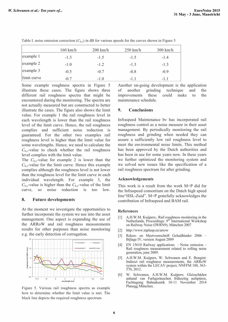
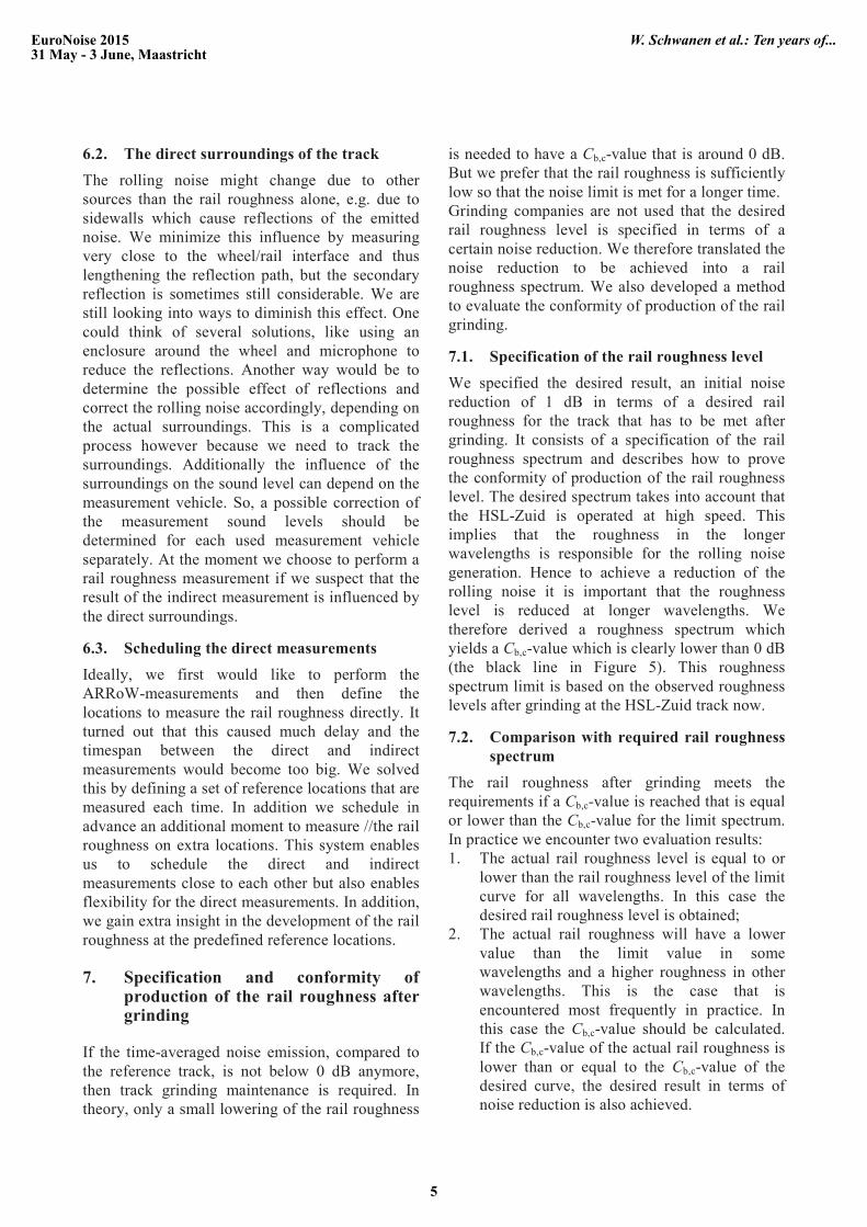
Some example roughness spectra in Figure 5 illustrate these cases. The figure shows three different rail roughness spectra that might be encountered during the monitoring. The spectra are not actually measured but are constructed to better illustrate the cases. The figure also shows the limit value. For example 1 the rail roughness level in each wavelength is lower than the rail roughness level of the limit curve. Hence, the rail roughness complies and sufficient noise reduction is guaranteed. For the other two examples rail roughness level is higher than the limit value for some wavelengths. Hence, we need to calculate the Cb,c-value to check whether the rail roughness level complies with the limit value. The Cb,c-value for example 2 is lower than the Cb,c-value for the limit curve. Hence this example complies although the roughness level is not lower than the roughness level for the limit curve in each individual wavelength. For example 3, the Cb,c-value is higher than the Cb,c-value of the limit curve, so noise reduction is too low.

8. Future developments

At the moment we investigate the opportunities to further incorporate the system we use into the asset management. One aspect is expanding the use of the ARRoW and rail roughness measurements results for other purposes than noise monitoring e.g. the early detection of corrugation.

Another on-going development is the application of another grinding technique and the improvements these could make to the maintenance schedule.

9. Conclusions

Infraspeed Maintenance bv has incorporated rail roughness control as a noise measure in their asset management. By periodically monitoring the rail roughness and grinding when needed they can assure a sufficiently low rail roughness level to meet the environmental noise limits. This method has been approved by the Dutch authorities and has been in use for some years now. In these years we further optimized the monitoring system and we solved new issues like the specification of a rail roughness spectrum for after grinding.

Acknowledgements This work is a result from the work M+P did for the Infraspeed consortium on the Dutch high speed line“HSL-Zuid”. M+P gratefully acknowledges the contribution of Infraspeed and BAM rail.

References [1] A.H.W.M. Kuijpers,: Rail roughness monitoring in the

Netherlands, Proceedings: 9th International Workshop on Railway Noise (IWRN9), München 2007

[2] http://www.mplusp.eu/arrow[3] Reken- en Meetvoorschrift Geluidhinder 2006 –

Bijlage IV, version August 2009 [4] EN 15610 Railway applications - Noise emission –

Rail roughness measurement related to rolling noise generation, june 2009.

[5] A.H.W.M. Kuijpers, W. Schwanen and E. Bongini: Indirect rail roughness measurements, the ARRoW system within the LECAV project, NNFFM 188, 563-570, 2012.

[6] W. Schwanen, A.H.W.M. Kuijpers: Gleisschäden anhand van Farhgeräuschen frühzeitig aufspüren, Fachtagung Bahnakustik 10-11 November 2014 Planegg München.

Table I. noise emission correction (Cb,c) in dB for various speeds for the curves shown in Figure 5

160 km/h 200 km/h 250 km/h 300 km/h example 1 -1.3 -1.5 -1.5 -1.4example 2 -1.0 -1.2 -1.3 -1.3 example 3 -0.5 -0.7 -0.8 -0.9limit curve -0.7 -1.0 -1.1 -1.1

Figure 5. Various rail roughness spectra as example how to determine whether the limit value is met. The black line depicts the required roughness spectrum

-20

-10

0

10

20

31.5 16 8 4 2 1 0.5 0.25

roug

hnes

s le

vel [

dB re

1]

wavelength [cm]

example 1 example 2

example 3 limit value



6

ten years of rail roughness control in the netherlands ... et...ten years of rail roughness control...

Documents