ten-year retrospective summary report - fpc year retrospective rep… · ten-year retrospective...

COMPARATIVE SURVIVAL STUDYTen-year Retrospective Summary

Report

Presentation to theIndependent Scientific Advisory Board

September 14, 2007

CSS Authors:• Howard Schaller, Paul Wilson, and Steve Haeseker, U.S. Fish and

Wildlife Service

• Charlie Petrosky, Idaho Department of Fish and Game

• Eric Tinus and Tim Dalton, Oregon Department of Fish and Wildlife

• Rod Woodin, Washington Department of Fish and Wildlife

• Earl Weber, Columbia River Inter-Tribal Fish Commission

• Nick Bouwes, EcoLogic

• Thomas Berggren, Jerry McCann, Sergei Rassk, Henry Franzoni, and Pete McHugh, Fish Passage Center

Project Leader: Michele DeHart, Fish Passage Center

CSS Background• 1996 by states, tribes & FWS to estimate survival rates

at various life stages

• Develop a more representative control for transport evaluations

• Compare survival rates for Chinook from 3 regions

• Information derived from fish PIT tagged above dams

• Collaborative process implemented for design and analyses

• Project reviewed (ISAB, ISRP, etc.) and modified– focusing on CIs about survival estimates– documenting methods

CSS joint project of the state, tribal, and federal fishery managers

Final ReportPosted on BPA and FPC websites

ReviewRegional Review public reviewDrafts posted on FPC and BPA websites

AnalysisCSS Oversight Committee, FPC - coordinates

Data PreparationFPC

ImplementationFPC - logistics, coordination, e.g.PITAGIS - data management

ReviewRegional review, ISAB, ISRP, FPAC, NMFS

DesignWDFW, CRITFC, USFWS, ODFW, IDFG

Objectives

• CSS evaluates two aspects of transportation – empirical SARs compared to those needed for survival and

recovery (NPCC 2-6% objective)– SAR comparisons between transport and in-river migration

routes

• Evaluate effects of the hydrosystem on Snake River populations – evaluate environmental conditions & hydro operations on in-river

survivals– compare Snake & downriver population performance

• evaluate biological differences between groups – indirect hydrosystem effects on estuary/early ocean life stage

Tasks• Develop long-term index of transport and in-river

survival rates for Snake River wild and hatchery spring/summer Chinook and steelhead– Mark at hatcheries > 220,000 PIT tags– Smolts diverted to bypass or transport from study design– In-river groups SARs from never detected & detected > 1 times– SARs from Below Bonn for Transported & In-river groups

(TIR and Differential delayed mortality-D)– Increase marks for wild Chinook to compare hatchery & wild Chinook

> 23,000 added wild PIT tagged fish– Begin marking of steelhead populations in 2003

• Develop long-term index of survival rates from release to return

• Compare overall survival rates for upriver and downriver spring/summer Chinook hatchery and wild populations

• Provide a time series of SARs for use in regional long-term monitoring and evaluation

What does CSS project provide?• Long-term consistent information collaboratively

designed and implemented• Information easily accessible and transparent• Long-term indices:

– Travel Times– In-river Survival Rates– In-river SARs by route of passage– Transport SARs

• Comparisons of SARs– Transport to In-River– By geographic location– By hatchery group– Hatchery to Wild– Chinook to Steelhead

2006 ISAB Review

• Conclusions:– Council should view the CSS as a good long-

term monitoring program - results should be viewed with increasing confidence

– Project has received a high level of independent and outside review

– Definitely worth funding

ISAB/ISRP Recommendations• CSS produce a ten-year summary report

– in-depth description of methods and analyses• consolidate descriptions in the ten-year summary

– interpretation of the data in a retrospective style • include key data and summaries in report or appendices

• Test assumptions inherent in the analyses

• Emphasize more diverse metrics of differential survival

• Analyses by grouping data for environmental and operational factors

• Evaluate size at release on survival of PIT-tagged fish

• Do PIT-tagged fish survive as well as untagged fish?

• Pre-assigning the intended routes of passage at the time of release

• Add more downriver sites in the future

Organization of Presentation

• Overview & Background• ISAB Recommendations• Chapter by Chapter

– Overview – Key questions & ISAB recommendations– Methods & results– Response to Regional Review– Conclusions

• Overall Conclusions & Future

Chapters

1. Introduction, Overview, & Organization

2. Travel Time, Survival, and Instantaneous Mortality Rates

3. Annual SAR by Study Category, TIR, SR, and D

4. Estimating Environmental Stochasticity in SARs, TIRs and Ds

5. Evaluation and Comparison of Overall SARs

6. Partitioning Survival Rates-Hatchery release to return

7. Simulation Studies to Explore Impact of CJS Model Assumption

8. Conclusions & Future Direction

AppendicesA. Logistical Methods

B. Analytical Methods: Statistical Framework

C. 2006 Design and Analysis Report

D. Tables of PIT-Tag Marking Data

E. Groups of PIT-tagged Chinook and Steelhead SARs

F. Cumulative passage distributions

G. Comments and Response from ISRP/ISAB

H. Response to Comments - DRAFT CSS 10 Year Report

Rationale:

• ISAB 2006-3: “The data could be aggregated to more closely meet the needs of hydrosystem managers…as data are accumulated over more years, it may be feasible to partition analyses into environmental or operational categories across years to obtain more functional correlations.”

• CSS objective to characterize fish responses

• ISAB 2003-1: “An interpretation of the patterns observed in the relation between reach survival and travel time or flow requires an understanding of the relation between reach survival, instantaneous mortality, migration speed, and flow.”

Chapter 2 - Contents

• Retrospective summary of fish travel time, survival, and instantaneous mortality rates, both within- and across-years

• Develop models characterizing the associations between environmental and management factors and fish responses

• Evaluate three approaches for modeling survival rates

ISAB recommendations addressed in Chapter 2

• Detailed analyses and interpretation of the data in a retrospective style

• Analyze data with respect to environmental and operational factors

• Supplement annual analyses with finer-scale analyses

Methods:

• Two reaches: LGR-MCN (CHW, CHH, STH&W)MCN-BON (CHH&W, STH&W)

Instantaneous mortality rate

• Evaluated models using AICc and BIC

• Weekly release cohorts of PIT-tagged fish

• Estimated median fish travel time (FTT) and survival rate

Environmental and Management Factors:

• Temperature

• Turbidity

• Flow (kcfs)

• Flow -1

• Water travel time (WTT, days)

• Average percent spill

• Seasonality (Julian Day)

0

5

10

15

20

25

30

35

40

1998 20070

5

10

15

20

25

1999 2007

Yearling Chinook median fish travel times

1998 2000 2002 2004 2006 2000 2002 2004 2006

LGR-MCN MCN-BON

r2 = 0.89 r2 = 0.95

Environmental and management factors: WTT, percent spill, Julian day

0

5

10

15

20

25

30

1998 20070

2

4

6

8

10

12

14

16

18

1999 2007

Steelhead median fish travel times

LGR-MCN MCN-BON

1998 2000 2002 2004 2006 2000 2002 2004 2006

Environmental and management factors: WTT, percent spill, Julian day

r2 = 0.90 r2 = 0.91

0

10

20

30

40

50 100 150 200 250

min. spill50% spillobserved

0

10

20

30

40

50 100 150 200 250

0

10

20

30

40

50 100 150 200 250

FTT

Flow

Chinook

Early

Late

0

10

20

30

50 100 150 200 250

min. spill50% spillObserved

0

10

20

30

50 100 150 200 250

0

10

20

30

50 100 150 200 250

steelheadLGR-MCN

Instantaneous mortality

Exponential law of population decline:

tZt eSNN ⋅−==

0

Rearranging:

tSZ e )(log−

=t

SZ e )ˆ(logˆ −=ML estimate of Z:

In this application:

MCNLGR

MCNLGReMCNLGR TTF

SZ−

−−

−= ˆ

)ˆ(logˆ

0.00

0.05

0.10

0.15

0.20

1998.0 2007.00.00

0.05

0.10

0.15

0.20

1999 2007

Yearling Chinook instantaneous mortality rates (Z)

LGR-MCN MCN-BON

1998 2000 2002 2004 2006 2000 2002 2004 2006

Factors: WTT, Julian day Factors: Julian day

r2 = 0.48 r2 = 0.15

0.00

0.10

0.20

0.30

0.40

19990.00

0.10

0.20

0.30

0.40

1998.00

Steelhead instantaneous mortality rates (Z)

LGR-MCN MCN-BON

2000 2002 2004 2006

Factors: flow -1, Julian day, spill Factors: temperature

r2 = 0.54 r2 = 0.51

1998 2000 2002 2004 2006

CHW STH&W CHH&W STH&WDaily percent mortality (mean Z) 3.0% 6.7% 6.4% 10.6%

MCN-BONLGR-MCN

Daily percent mortality by species and reach:

0.00

0.02

0.04

0.06

0.08

0.10

0.12

90 100 110 120 130 140 150

5 d10 d15 d20 d

Julian day

Predicted

LGR-MCN Z

wild Chinook

0.00

0.02

0.04

0.06

0.08

0.10

0.12

90 100 110 120 130 140 150

5 d10 d15 d20 d

Julian day

Predicted

LGR-MCN Z

wild Chinook

April May

Predicted relationship for instantaneous mortality

0.00

0.02

0.04

0.06

0.08

0.10

0.12

0.14

0.16

105 115 125 135 145

75 kcfs / 0% spill

75 kcfs / 40% spill

150 kcfs / 45% spill


H&W steelhead

Julian day

Predicted

LGR-MCN Z

0.00

0.02

0.04

0.06

0.08

0.10

0.12

0.14

0.16

105 115 125 135 145

75 kcfs / 0% spill

75 kcfs / 40% spill



H&W steelhead

Julian day

Predicted

LGR-MCN Z

Predicted relationship for instantaneous mortality

April May

Survival

Evaluated three approaches:Standard survival approach

Constant Z survival approach

Variable Z survival approach

...)(log 22110 +⋅+⋅+= XXSe βββ...)ˆˆˆ(* 22110 +⋅+⋅+= XXeS βββ

** FTTZeS ⋅−=

*** FTTZeS ⋅−=

Survival approach comparison - Results

variable Z > standard >> constant Z

Variable Z approach had best RMSE and R2 values in 4 of 5 cases and best AIC in 2 of 5 cases

Standard approach had fewest parameters and best AIC in 3 of 5 cases

Variable Z approach accounted for 51-80% (64% on average) of the variation in survival rates

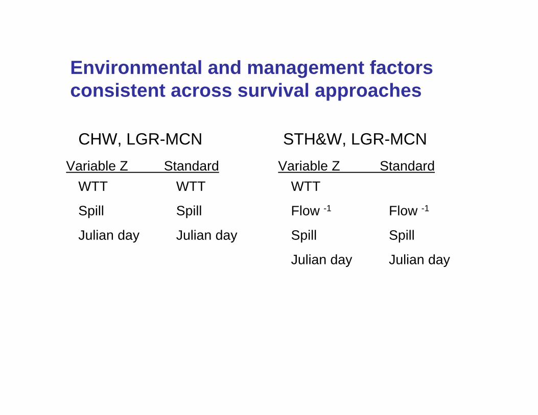
Environmental and management factors consistent across survival approaches

CHW, LGR-MCN STH&W, LGR-MCNVariable Z StandardVariable Z Standard

WTT WTT

Spill Spill

Julian day Julian day

WTT

Flow -1 Flow -1

Spill Spill

Julian day Julian day

Yearling Chinook survival

0.2

0.4

0.6

0.8

1.0

1.2

1998.0 2007.00.2

0.4

0.6

0.8

1.0

1.2

19991998 2000 2002 2004 2006 2000 2002 2004 2006

LGR-MCN MCN-BON

r2 = 0.63 r2 = 0.51

0.0

0.2

0.4

0.6

0.8

1.0

1.2

19990.0

0.2

0.4

0.6

0.8

1.0

1.2

1998

steelhead survival

1998 2000 2002 2004 2006 2000 2002 2004 2006

LGR-MCN MCN-BON

r2 = 0.80 r2 = 0.71

0.2

0.4

0.6

0.8

1.0

50 100 150 200 250

0.2

0.4

0.6

0.8

1.0

50 100 150 200 250

0.2

0.4

0.6

0.8

1.0

50 100 150 200 250

min. spill50% spillobserved

Early

Late

Chinook

S

0.0

0.2

0.4

0.6

0.8

1.0

50 100 150 200 250

min. spill50% spillObserved

0.0

0.2

0.4

0.6

0.8

1.0

50 100 150 200 250

0.0

0.2

0.4

0.6

0.8

1.0

50 100 150 200 250

steelheadLGR-MCN

Flow

S

Flow

Regional review comments

Instantaneous mortality (Z)

Mathematically the analysis based on Z is invalid

Z is biased

Analyses based on Z should be deleted from the report

PIT-tag data are incapable of estimating instantaneous mortality rates

In fact, trends in Z are nothing more than inverse trends in travel times misinterpreted or misconstrued as survival effects

Z is independent of survival

Problems are encountered when Z is related to a variety of factors

Actions to decrease FTT would increase Z

0.00

0.05

0.10

0.15

0.20

0 5 10 15 20 25

0.00

0.05

0.10

0.15

0.20

0 5 10 15 20 25

0.00

0.05

0.10

0.15

0.20

0 5 10 15 20 25

0.00

0.02

0.04

0.06

0.08

0.10

5 10 15 20 25 30

0.00

0.02

0.04

0.06

0.08

0.10

5 10 15 20 25 30

0.00

0.02

0.04

0.06

0.08

0.10

5 10 15 20 25 30

instantaneous

mortality (Z)

Chinook steelheadEarly

Late

LGR-MCN

FTT FTT


Results

Eliminate 20-d WTT curve from graph

CSS model is incapable of capturing the pattern of survival in 2001

0.0

0.2

0.4

0.6

0.8

1.0

2001 2001.5 2002 2002.5 2003 2003.5 2004

Survival

LGR-MCN

2001

STH

CHW CHH

Conclusions

Juvenile travel times, instantaneous mortality rates, and survival rates through the hydrosystem are strongly influenced by managed river conditions including flow, water travel time, and spill levels.

Statistical relationships were developed that can be used to predict the effects of environmental factors and management strategies on migration and survival rates of juvenile yearling Chinook and steelhead.

Analyses indicate that improvements in in-river survival and travel times can be achieved through management actions that reduce water travel time or increase the average percent spilled. The effectiveness of these actions varies over the migration season.

Chapter 3

Annual SAR by Study Category, TIR, SR, and D: Patterns and

Significance

2

Chapter 3 ‐ OverviewEstimate and compare annual SARs for hatchery and wild groups of smolts with different hydrosystem experiences (T0, C0, C1 groups)Evaluate effectiveness of transportation relative to in-river migration via annual SAR ratios between T0 and C0 fish (TIR)Partition differential survival of transported & in-river fish by estimating SR and D

3

ISAB recommendations addressed in Chapter 3 & Appendices B‐E

In-depth description of methods and detailed analyses and interpretation of data in a retrospective style Consolidate and effectively present methodologies used in analyses, clarifying notationShow key data and data summaries in body of report or appendicesInvestigate potential bias of analytical approaches

4

Chapter 3 ‐MethodsCJS method for in-river survival rate estimates, with extrapolation when necessaryEstimation of number of smolts in study categories, and resulting SARs describedEstimation of TIR and DBootstrap program to estimate confidence intervals around Ss, SARs, TIRs, and Ds (Appendix B)Detailed statistical framework & equations in Appendix B, with table showing timeline of method developmentMethodology for obtaining unbiased TIRs (Appendix C)

5

Results: Appendices D and E tables

Appendix D: supporting tables of PIT-tag data and estimates of major parameters for analyses presented in Chapters 3,4,5,& 6Appendix E: Initial estimates, std devs, CIsfrom bootstrap program for major parameters, organized by Species, Rear-type and Migration Year

6

Results: T0 and C0 SARsWild Spring/Summer Chinook

0.000

0.005

0.010

0.015

0.020

0.025

0.030

0.035

0.040

19941995199619971998199920002001200220032004

Migration Year

SAR

Est

imat

e

sarT0sarC0

Wild Steelhead

0.00

0.01

0.02

0.03

0.04

0.05

1997 1998 1999 2000 2001 2002 2003Migration Year

SAR

Est

imat

e

sarT0sarC0

7

Results: Comparing wild and hatchery Chinook SARs

8

Results: Wild Chinook TIRs and Ds

Wild Chinook TIR

0

1

2

3

4

5

6

7

1994 1995 1996 1997 1998 1999 2000 2001 2002 2003 2004

Migration Year

SAR 2

(T0)

/SA

R(C

0)

16.8

Wild Chinook D

0

1

2

3

19941995199619971998199920002001200220032004Migration Year

Estim

ate

of D

4.2

9

Results: Wild steelhead TIRs and DsWild Steelhead TIR

0

1

2

3

4

5

6

7

8

9

10

1997 1998 1999 2000 2001 2002 2003

Migration Year

SAR

2(T 0

)/SA

R(C

0) 37

Wild Steelhead D

0

1

2

3

4

5

1997 1998 1999 2000 2001 2002 2003

Migration Year

D E

stim

ate

5.87

10

Results: Wild vs. hatchery SRSR for Hatchery and Wild Steelhead

0

0.1

0.2

0.3

0.4

0.5

0.6

0.7

1997 1998 1999 2000 2001 2002 2003

S RWildHatchery

Hatchery & Wild Chinook SR

0.1

0.2

0.3

0.4

0.5

0.6

0.7

0.8

1994 1995 1996 1997 1998 1999 2000 2001 2002 2003 2004

S R

WildDWORRAPHMCCAIMNACATH

11

Results: Steelhead vs. Chinook SRSR for Wild Steelhead and Wild Chinook

0.0

0.1

0.2

0.3

0.4

0.5

0.6

0.7

1997 1998 1999 2000 2001 2002 2003

S R

SteelheadChinook

12

Results: Comparing hatchery and wild TIR

Hatchery & Wild Chinook

-1.0

-0.5

0.0

0.5

1.0

1.5

2.0

2.5

3.0

3.5

1994 1995 1996 1997 1998 1999 2000 2001 2002 2003 2004

ln(T

IR)

WildDWORRAPHMCCAIMNHCATH

Hatchery and Wild Steelhead

-2

-1

0

1

2

3

4

5

1997 1998 1999 2000 2001 2002 2003

ln(T

IR)

WildHatchery

13

Regional Review commentsComment: Bootstrap confidence intervals not superior to theoretical normal CIs from mark-recapture data analyzed with CJS modelResponse: Bootstrap for CIs was recommendation of ISAB − Bootstrap to produce CIs for more complex parameters− Parametric variance of S estimates used in Chapter 2 − Bootstrap CIs for reach S ≈ CJS CIs− Bootstrap CIs for several quantities were compared to estimates from profile likelihood in 2002 CSS Annual Report

14

Regional Review comments, cont.

Comment: Use of the geometric mean needs justification, since geometric mean will always be lower than the arithmetic meanResponse: TIR and D both represent ratios of survival rates, for which the ordering (numerator vs. denominator) is arbitrary− Example: two years of equal credibility, one with TIR = 5.0, other with TIR = 0.2− Zar (1984): “[The geometric mean] finds use in averaging ratios where it is desired to give each ratio equal weight”

15

Regional Review comments, cont.

Comment: Use of C1 fish would provide insight into temporal changes in return rates of transported and non-transported fishResponse: Temporal variation in SARs of transported and in-river fish is investigated using C1 fish in Chapter 4

16

Regional Review comments, cont.Comment: That SAR are lower than objectives provides no evidence that FCRPS related mortality is the reasonResponse: Efficacy of transportation-based recovery strategies cannot be judged only from TIR − Absolute values of SAR, or alternatively “hydrosystem survival”, must be considered− Other information, including historical Snake River SARs and downriver SARs, suggests FCRPS is a major factor in depressing SARs (e.g. Chapter 5)

17

Chapter 3: FindingsAnnual SARs for wild Chinook have been highly variable, but far below NPCC target rangeAnnual SARs for wild steehead higher, exceeding the lower end of NPCC target range 4/6 yearsLittle or no benefit of transporting wild Chinook in most years; CIs usually overlap 1 (2001 is exception)Transport beneficial most years most hatcheries (Chinook)Transport beneficial most years wild & hatchery steelhead

18

Chapter 3: Findings, cont.

CIs on TIRs and Ds wide most years; especially wide in 2001, with high point estimateLowest D values for wild Chinook; highest for wild steelheadHigher TIR values for wild steelhead (compared to wild Chinook) are due to both lower steelhead in-river survival and higher steelhead D.

19

Extras

20

Calculation of D

••

∗=⋅⋅

=T

R

T

R

SS

TIRSCSARSTSAR

D)()(

0

0

Chapter 4

Estimating environmental stochasticity in SARs, TIRs, and

Ds

Chapter 4 ‐ OverviewCan we get a better estimate of central tendency of SARs, TIRs, & Ds for wild fish, given large process error and large variation in sample size? Annual CIs of TIRs often overlap 1—can combining data from all years and removing sampling variance from SARslead to tighter distributions of TIR (and D)? Can covariance between annual estimates of SARs of transported and untransportedfish be incorporated to narrow CIs of TIR and D?

ISAB recommendations addressed in Chapter 4In-depth description of methods & detailed analyses and interpretation of data in a retrospective style Consolidate & effectively present method-ologies used in analyses, clarifying notationSupplement with analyses that group data on environmental or operational factors amenable to controlInvestigate potential bias of analytical approachesDiverse metrics – passage routes, # dams bypassed

Chapter 4 – Methods for SARsAssume SAR measurement error is independent binomial sampling errorUse method of Akçakaya (2002) – estimate & remove sampling variance from total varianceSample size influences mean, total variance, & sampling variance of time seriesFit resulting SAR mean and variance, reflecting environmental variance alone, to beta distribution (Morris & Doak 2002, Kendall 1998)

Chapter 4 – Methods for TIRs & Ds

Model ratio of resulting SAR distributions to get project-specific TIR distributionsInclude covariance between SAR(T) and SAR(C)—tends to reduce variance of ratioEstimating Ds: Need environmental variance distributions of SR

Multiply distribution of SR by TIR dist to get D distribution

Results: LGR TIR distributions

0

0.002

0.004

0.006

0.008

0.01

0.012

0.014

0 0.5 1 1.5 2 2.5 3

TIR

Prob

. den

sity

0

0.2

0.4

0.6

0.8

1

1.2

Cum

ulat

ive

den

sity

Prob. density Cumulative density TIR = 1

Wild Chinook (1994-2003)

0

0.0005

0.001

0.0015

0.002

0.0025

0.003

0.0035

0.004

0.0045

0 1 2 3 4 5 6

TIR

Prob

. den

sity

0

0.2

0.4

0.6

0.8

1

1.2

Cum

ulat

ive

den

sity

Prob. density Cumulative density TIR = 1

Wild steelhead (1997-2002)

Results: LGR D distributions

0

0.005

0.01

0.015

0.02

0.025

0.03

0 0.5 1 1.5 2

D

Prob

. den

sity

0

0.2

0.4

0.6

0.8

1

1.2

Cum

ulat

ive

dens

ity

Prob. density Cumulative density

0

0.001

0.002

0.003

0.004

0.005

0.006

0.007

0.008

0.009

0.01

0 0.5 1 1.5 2 2.5 3

D

Prob

. den

sity

0

0.2

0.4

0.6

0.8

1

1.2

Cum

ulat

ive

dens

ity

Prob. density Cumulative density

Wild Chinook Wild steelhead

Results: Overall SAR distributions

0

0.2

0.4

0.6

0.8

1

1.2

0% 1% 2% 3% 4% 5% 6% 7% 8% 9% 10%

SAR

Rel

ativ

e Pr

ob. d

ensi

ty

Overall SAR

Target Range

Target Range

`

0

0.2

0.4

0.6

0.8

1

1.2

0% 1% 2% 3% 4% 5% 6% 7% 8% 9% 10%

SAR

Rel

ativ

e Pr

ob. d

ensi

ty Overall SAR

Target Range

Target Range

`

Wild Chinook Wild steelhead

Within season variation in SARs ‐Chinook

0

0.1

0.2

0.3

0.4

0.5

0.6

0.7

0.8

0.9

1

0 0.01 0.02 0.03 0.04 0.05 0.06 0.07 0.08

SAR

Den

sity

Early

Middle

Late`

0

0.1

0.2

0.3

0.4

0.5

0.6

0.7

0.8

0.9

1

0 0.01 0.02 0.03 0.04 0.05 0.06 0.07 0.08

SAR

Den

sity

Early

Middle

Late`

Transported from LGR In-river from LGR (C1)

Within season variation in SARs ‐Steelhead

Transported from LGR In-river from LGR (C1)

0

0.1

0.2

0.3

0.4

0.5

0.6

0.7

0.8

0.9

1

-0.01 0.01 0.03 0.05 0.07 0.09 0.11 0.13 0.15

SAR

Den

sity

Early

Middle

Late

`

0

0.1

0.2

0.3

0.4

0.5

0.6

0.7

0.8

0.9

1

0 0.01 0.02 0.03 0.04 0.05 0.06 0.07 0.08 0.09 0.1 0.11 0.12 0.13 0.14 0.15

SAR

Den

sity

Early

Middle

Late

`

Effect of detection history on in‐river SAR – wild Chinook

Probability density functions of C0 and C1 SARs of wild chinook for migration years 1994-2002

0

0.1

0.2

0.3

0.4

0.5

0.6

0.7

0.8

0.9

1

0% 1% 2% 3% 4% 5% 6% 7% 8% 9% 10%

SAR

Rel

ativ

e Pr

ob. d

ensi

ty

C0

C1`

Regional Review commentsComment: Akçakaya method inappropriate for mark-recapture; should use Gould and Nichols (1998) approachResponse:

G&N deal with two sources of “sampling” variabilityIn CSS, no sampling variance of the first kind, since

all survivors “recaptured” by PIT-tag detection at LGR —only demographic stochasticity

Therefore, more involved methods of G&N for estimating the first kind of sampling variance and its covariance with the second kind are not required

Sampling variance in estimate of C0 addressed next

Regional Review comments, cont. Comment: SARs do not have a binomial sampling variance, for both the numerator and denominator (i.e., C0 fish) are estimated random variables.

Response: Numerator of each SAR is count of PIT-

tagged fish with relevant capture historyEffect of variance in C0 can be

investigated, using:

YXY

X

Y

XY

Y

X

YXVar σρσ

μμ

μσ

σμμ

⎟⎟⎠

⎞⎜⎜⎝

⎛−+⎟⎟

⎠

⎞⎜⎜⎝

⎛≅⎟

⎠⎞

⎜⎝⎛

32

22

4

2

2

Regional Review comments, cont. Response cont.:

Estimated actual sampling variance for 2 C0 estimates: 1) lowest C0, highest CV; 2) highest C0, lowest CV

Binomial variance very slightly overestimates actual sampling variance of SAR(C0)Mean C0

CV of C0

SAR est.

ρ Actual variance

Actual CV

Binomial variance

Binomial CV

103 10% 2.91% 0.17 2.66 x 10-4 56% 2.74 x 10-4 57% 8879 1.5% 0.33% 0.08 3.68 x 10-7 18% 3.70 x 10-7 18%

Regional Review commentsComment: Estimated demographic variance is greater than total variance [for steelhead transported from LMN], suggesting something is wrong and thus casting doubt on all methods and results in this chapter

Response: Gould and Nichols (1998) found estimated sampling

variance > total variance for a number of their sample data sets

G&N reference literature indicating that negative estimates of variance are not uncommon in the variance components literature

Consequence of large sampling variation due to low # of PIT-tagged steelhead transported from LMN

Used observed inter-annual variance as an estimate of environmentally driven variance

Regional Review commentsComment: Such small transport groups [PIT-tagged steelhead] produce unreliable parameter estimates that can seriously distort interpretation of results

Response: Uncertainty in parameter estimates explicitly

estimated and accounted for Chapter 4 procedures

Effects of small sample sizes seen in the resultant wide confidence intervals for SARs of LGS- and LMN-transported steelhead

Effect of this uncertainty is carried into estimates of TIR and D for these projects and explicitly presented

Chapter 4 ‐ ConclusionsRealized SARs have been considerably below NPCC target range for Chinook, and generally below for steelheadTransportation as currently implemented does not benefit wild Chinook (compared to in-river migrating C0 fish)Transportation, especially from LGR, appears to benefit wild steelheadSubstantial delayed mortality of transported wild ChinookLower, more uncertain levels of delayed mortality for transported wild steelhead

Chapter 4 – Conclusions, cont.Patterns in decline in SAR of in-river (C1) of both species as the migration season progresses consistent with hypothesis of delayed mortality of in-river fish due to protracted migrationPattern of SARs over season suggests that Chinook TIRs could be improved by delaying transportation until later in season, but also that maximizing SARs of both wild steelhead and Chinook cannot be accomplished through transportation*

*Unless steelhead SR and/or Chinook can be separated from steelhead before barging

Comparative Survival Study Chapter 5

Evaluation and Comparison of Overall Smolt-to-Adult Return

Rates

Chapter 5 - Contents• Wild vs. hatchery SAR trends

• Compare wild SARs to NPCC 2 to 6% SAR objectives– evaluate the overall effectiveness of F & W program– evaluate effectiveness of the transportation program

• Compare wild Mid-Columbia (downriver) to Snake River Chinook populations – is the upriver/downriver difference in SARs consistent with differential

mortality from spawner-recruit data?

• Compare biological characteristics of upriver and downriver populations

• Compare downriver and Snake River hatchery SARs

• Examine relationships of wild Chinook SARs to ocean and river conditions



• Add more downriver sites in the future

• Specific section in the report focusing on the potential effectsof size at release on survival of all PIT-tagged fish

• Analyze survival data with respect to environmental and operational factors

• Analyses could emphasize more diverse metrics of differential survival

• Evaluate if PIT-tagged fish survive as well as untagged fish

Snake River wild Steelhead

0.0%

1.0%

2.0%

3.0%

4.0%

5.0%

6.0%

7.0%

1997 1998 1999 2000 2001 2002 2003

Migration year

SAR

90% UL

Bootstrap average90% LL

2% NPCC Objective6% NPCC Objective

Retrospective AnalysisSnake Wild Populations

Wild Snake River spring/summer Chinook

0.0%

1.0%

2.0%

3.0%

4.0%

5.0%

6.0%

7.0%

1994 1996 1998 2000 2002 2004Migration year

SAR

90% ULBootstrap average90% LL2% NPCC Objective6% NPCC Objective

Snake River spring/summer Chinook

0.0%

1.0%

2.0%

3.0%

4.0%

1994 1996 1998 2000 2002 2004Migration year

SAR

Wild

DWOR

RAPH

MCCA

IMNA

CATH

Retrospective AnalysisSnake Hatchery & Wild Populations

McCall hatchery Chinook

0.0%

1.0%

2.0%

3.0%

4.0%

1997 1998 1999 2000 2001 2002 2003 2004Migration year

SAR

90% UL

Bootstrap average

90% LL

2% minimum

Snake River vs Downriver Wild Chinook

Snake vs. John Day wild stream-type Chinook (PIT tags)

0.0%

2.0%

4.0%

6.0%

8.0%

10.0%

12.0%

14.0%

1999 2000 2001 2002 2003 2004 2005Migration year

SAR

(1st

dam

to B

ON)

Snake

John Day

NPCC 2-6% SAR

PIT tag studies:Downriver SARs are 3-4X Snake SARsSnake River SARs generally < 2 to 6% SAR

Spawner-Recruit analysis vs SAR comparisons:estimated differential mortality estimated differential mortality -- Snake vs. downriverSnake vs. downriver

Differential mortality

-1.0

0.0

1.0

2.0

3.0

4.0

5.0

1970 1975 1980 1985 1990 1995 2000 2005

Migration year

Diff

eren

tial m

orta

lity

Spawner-recruit

PIT tags

Comparison of Biological Characteristics for Snake and Downriver stream-type wild

Chinook populations

Juvenile Length Distribution for Snake vs downriver wild Chinook populations

2000

CLWTRP

GRNTRP

IMNTRPJD

AR1

SALTRP

SNKTRP

Release Site

75

100

125

150

Fork

Len

gth

(mm

)

2001

CLWTRP

GRNTRP

IMNTRPJD

AR1

SALTRP

SNKTRP

Release Site

75

100

125

150

Fork

Len

gth

(mm

)

2002

CLWTRP

GRNTRP

IMNTRPJD

AR1

SALTRP

SNKTRP

Release Site

75

100

125

150

Fork

Len

g th

(mm

)

2003

CLWTRP

GRNTRP

IMNTRPJD

AR1

SALTRP

SNKTRP

Release Site

75

100

125

150

Fork

Len

gth

(mm

)

2004

CLWTRP

GRNTRP

IMNTRPJD

AR1

SALTRP

SNKTRP

Release Site

75

100

125

150

Fork

Len

gth

(mm

)

2005

CLWTRP

GRNTRP

IMNTRPJD

AR1

SALTRP

SNKTRP

Release Site

75

100

125

150

Fork

Len

g th

(mm

)

Juvenile Chinook emigration distributions for Snake vs downriver

populations

70 80 90 100 110 120 130 140 150Julian date

0.0

0.1

0.2

0.3

0.4

0.5

0.6

0.7

0.8

0.9

1.0

Cum

ulat

i ve

p ass

a ge

SNKTRPSALTRPJDAR1IMNTRPGRNTRPCLWTRP

Release Site

Wild Chinook salmon smolt downriver migration rates2000

0

10

20

30

40

CLWTRP GRNTRP IMNTRP JDAR1 SALTRP SNKTRP

release site

Mig

ratio

n ra

te (k

m /

d)2001

0

10

20

30

40


release site

Mig

ratio

n ra

te (k

m /

d)

2002

0

10

20

30

40


release site

Mig

ratio

n ra

te (k

m /

d)

2003

0

10

20

30

40


release siteM

igra

tion

rate

(km

/ d)

2004

0

10

20

30

40


release site

Mig

ratio

n ra

te (k

m /

d)

2005

0

10

20

30

40


release site

Mig

ratio

n ra

te (k

m /

d)

First-to-third dam migration duration as a function of water travel time

0 5 10 15 20Water travel time (days)

0

5

10

15

20Fi

rst-t

o-th

ird d

a m m

igra

tion

(day

s)


Release site

Estuary arrival timing distributions

100 120 140 160 180 200Julian date

0.0

0.2

0.4

0.6

0.8

1.0C

umul

ativ

e pa

ssa g

e


Release Site

* Snake River Water Travel Time (Lewiston-Bonneville): pre-dam less than 3 days and present condition 10-40 days

Biological Characteristics for Snake vs Downriver wild Chinook Populations

• No evidence for difference in size-at-migration existing

• No evidence for differences in departure from natal streams – evidence for greater variation in outmigration timing for upriver

populations

• No evidence for differences in smolt migration rates – rates were a function of water travel velocity

• Despite similar size, emigration timing, and downriver migration rate, Snake River smolts arrived at the estuary later (~7-10 days) than downriver populations

• Given similarities in biological characteristics and the increase in water travel times due to hydropower, discrepancy in arrival timing at BON for Snake River vs downriver populations is likely a result of the FCRPS

SARs for Snake River and John Day River wild Chinook for smolts passing Bonneville Dam during the

same period

SAR for Bonneville arrivals Apr 16 - May 31

0%

2%4%

6%8%

10%12%

14%

2000 2001 2002 2003Migration year

SAR

(BO

N-B

ON

)

C0C1T0John Day

Estimated differential mortality - Snake vs. downriverhatchery and wild populations

Differential mortality: wild and hatchery Chinook

-2.0

-1.0

0.0

1.0

2.0

3.0

2000 2001 2002 2003 2004

Migration year

Diff

eren

tial m

orta

lity

wildDWORRAPHMCCAIMNACATH

Multiple Regression Analysis: SARs vsmigration and ocean/climatic indices

Snake River spring/summer Chinook Smolt-to-Adult Return Rates (SAR)

0%

1%

2%

3%

4%

5%

6%

7%

1960 1965 1970 1975 1980 1985 1990 1995 2000 2005

Migration year

Preh

arve

st S

AR

run reconstruction adult recruits

CSS

NPCC objective 2%

NPCC objective 6%

Water Travel Time: Lewiston to Bonneville Dampre-dam ~2 days;

current ~ 19 days (10-40 days)

1938 (BON), 1953 (MCN), 1957 (TDD), 1961 (IHR), 1968 (JDA), 1969 (LMN), 1970 (LGS), 1975 (LGR)

05

1015202530354045

1929 1939 1949 1959 1969 1979 1989 1999

Wat

er T

rave

l Tim

e (d

ays)

Coastal Upwelling Process

•Pacific Decadal Oscillation

• Interdecadal climate variability in the North Pacific – (Sea Surface Temperature)

•Coastal Upwelling Index• based upon Ekman'stheory of mass transport due to wind stress - 45oN – (productivity)

“Good Ocean”• Cool phase PDO• April Upwelling • Oct Nov Downwelling

0.00

0.01

0.02

0.03

0.04

0.05

0.06

0.07

0 5 10 15 20 25 30 35 40Water Travel Time

SAR

average PDO & Upwell

good ocean SepPDO = -1; NovUp = -116

poor ocean SepPDO = 1; NovUp = -33

Expected change in SARsvs. WTT, PDO & Upwelling

Response to WTT - similar to results using upriver/downriver populations

Best fit (adj. R2=0.64), best 3 parameter model

Current WTT

Pre-dam WTT

Do PIT tag SARs represent SARs of the run at large?

• Run reconstruction (RR) SARsslightly larger than point estimate PIT SARs

• RR SARs fell within the 90% CIsof PIT SARs for 5 of the 8 years

• Unresolved issues with wild adult accounting for RR SARs

• Given unresolved issues for RR SARs, and lack of ability to place confidence bounds on RR SARs; assessing bias is difficult

• For analyses using ratios of SARs, this issue is of little concern

SARs: Run reconstruction vs. CSS PIT tag

0%

1%

2%

3%

4%

1994 1995 1996 1997 1998 1999 2000 2001 2002 2003 2004

Migration year

SAR

(LG

R-L

GR

)

SAR run reconstruction

90% LL

SAR CSS PIT

90% UL

Regional Review- Chapter 5• PIT Tag vs Run Reconstruction (RR) SARs

– Need more attention to evaluate discrepancies between PIT-tagged and untagged fish SARs

– Region needs to examine the assumptions and data adjustments to estimate SARs of untagged group

• resolution requires collaboration among several technical groups– RR SARs fell within the 90% CIs of PIT SARs for 5 of the 8 years– Not an issue for analyses using ratios of SARs– Identified tasks to help resolve this issue

• Delayed Mortality– investigated hypotheses for possible non-hydrosystem causes

(including hypotheses previously suggested by NWFSC) • consistent pattern of differential mortality across poor and favorable ocean conditions • estimates of in-river survival and relative survival of transported smolts• indirect evidence that the magnitude of delayed hydrosystem mortality is large• estimation of delayed or latent mortality (of in-river migrants) was not an objective of

CSS – SAR PIT-tag analyses provides independent estimates of differential

mortality, for comparison with published SR analyses• SAR estimates are free of assumptions related to the form of SR function• estimates are differential mortality - not delayed mortality

Regional Review- Chapter 5• Upriver/downriver population performance comparison

– a “natural” experiment – some design limitations

– addressed each past criticism for the upriver-downriver approach • compared biological characteristics of the two population groups• SARs ∼ 4-fold higher for downriver populations, none of the

biological characteristics exhibit differences to explain this level of differential mortality

– reviewers claim Bristol Bay data invalidate comparing performance of different populations from the same region

• BB sockeye salmon exhibit common annual survival patterns• correlations between stocks for BB ranged from 0.23 to 0.75

(geomean 0.44) • BB sockeye diversity attributed to varying challenges imposed by

freshwater spawning and rearing environments • CSS comparison extends SR analyses of differential mortality

using PIT-tag SARs, and life-history characteristics which may support alternative hypotheses of differential mortality - consistent with Hilborn et al. (2003)

Conclusions Chapter 5• SARs of Snake River wild spring/summer Chinook < NPCC

objective & met the 2% minimum 1 of 11 years

• SARs of Snake River wild steelhead < NPCC objective & met the 2% minimum 4 of 7 years

• SARs of hatchery spring/summer Chinook tracked closely with those of the aggregate Snake River wild population

• Higher Snake River wild spring/summer Chinook SARs were related to faster water travel time experienced during the smolt migration, cooler phases of the ocean, and stronger down-welling in the fall during the first year of ocean residence

• SARs of downriver wild spring Chinook ~ 4 X greater than Snake River SARs– consistent with previous findings of differential mortality derived

from spawner and recruit analyses – upriver and downriver hatchery spring/summer Chinook SARs

did not show the same level of differential mortality as wild

Conclusions Chapter 5• No evidence for consistent and/or systematic difference

between upriver and downriver wild Chinook salmon for the following biological characteristics: – size-at-migration, – tributary emigration timing – migration rates in the hydrosystem

• Delayed timing to the estuary of Snake River smolts due to the FCRPS

• Snake River SARs < downriver SARs when these wild Chinook populations arrived at the estuary during the same time period – disparity provides support for mechanisms of delayed

hydrosystem mortality in addition to alteration of estuary entry

Comparative Survival Study Chapter 6

Partitioning survival rates –hatchery release to return

Chapter 6 - Contents• Survival from hatchery release to LGR

• Adult survival from LGR to hatchery

• Detection of PIT adults at hatchery rack for transported and in-river groups

• Adult migration survival– Transport vs In-river groups– Relation to environmental and management indices



• Analyze survival data with respect to environmental and operational factors

Retrospective AnalysisHatchery release to LGR

0.00

0.20

0.40

0.60

0.80

1.00

1996 1998 2000 2002 2004 2006

Migration year

Surv

ival

(S1)

RAPH

DWOR

CATH

MCCA

IMNA

Proportion of PIT-tagged adults and jacks detected at LGR that were subsequently

detected at the hatchery racks

Expanded detection probability LGR adults to hatcheries

0.00

0.20

0.40

0.60

0.80

1.00

1996 1997 1998 1999 2000 2001 2002 2003

Smolt migration year

Expa

nded

LG

R -

HAT

de

tect

ion

prob

abili

ty

RAPH

DWOR

CATH

MCCA

Proportion of LGR adults and jacks detected at hatchery racks

0.00

0.10

0.20

0.30

0.40

0.50

0.60

1997 1998 1999 2000

Smolt migration year

Prop

ortio

n de

tect

ed

TransportIn-river

Percent of hatchery and wild adult Chinook salmon that were successful in migrating from

BON to LGR

50

60

70

80

90

100

LGR

LGSdownInrive

r

Suc

cess

ful (

%)

50

60

70

80

90

100

LGR

LGSdownInrive

r

Suc

cess

ful (

%)

Hatchery Wild

On average, 10% lower adult migration success for LGR transport

Parameter estimates for the top logistic regression model describing BON-LGR

migration success for CSS hatchery Chinook

Parameter Estimate SE T P-value Intercept 1.410 0.285 4.95 <0.001 LGR -0.446 0.092 -4.84 <0.001 LGSdown -0.212 0.123 -1.73 0.085 Spill -0.016 0.008 -2.04 0.041 Temperature 0.057 0.020 2.87 0.004

Transportation from LGR primary factor describing adult migration success

Regional Review- Chapter 6• NWFSC analysis found that unmarked hatchery Chinook salmon

returned at higher rates than PIT-tagged fish – Reviewers did not weight the C0 and T0 groups according to their actual

proportions for the run at large, and the C1 group is overrepresented in the NWFSC analysis

– SARs of the C1 group are substantially lower than those of C0, a negative bias

– Investigate potential issues of PIT-tag detection and recovery at hatchery weirs

• Pooling adult migration success data across juvenile migration year and return year - only if those factors are non-significant– CSS analyzed adult success on a year-by-year (migration or return) and

hatchery-specific basis – conclusions that outmigration experience was primary factor would not

change with formal test for year effects (a secondary factor) – logistic regression supports conclusion outmigration experience is

primary factor

Chapter 6 Conclusions• Adults transported from LGR as smolts exhibited 10%

lower upstream migration survival than either in-river or transported from LGS or LMO smolt history– logistic regression suggest lower passage rates for adults of

juvenile cohorts that migrated during periods of high spill and cold temperatures

• Increased straying may influence populations out of the Snake Basin (e.g. high out-of-basin strays into mid-Columbia steelhead and spring Chinook populations)

• Hatchery adult survival upstream of LGR was not associated with transport or in-river smolt histories

• Lack of evidence for a survival difference upstream of LGR indicates CSS SAR evaluations reasonably describe the relative performance of transported and in-river migrants

Comparative Survival Study

Chapter 7

Effects of CJS model assumption violations on parameter estimation

Background

CJS model used extensively within Region and in the CSS

A primary assumption of the CJS estimation methodology is that all members of a tagged group have a common underlying probability of survival and of collection at dams

Violations of this assumption could occur if survival or collection probabilities change over time

Objective was to explore how changes over time may influence CJS estimates, and CSS estimates that are used


Assumptions inherent in the analyses should be specifically tested, with continued vigilance toward avoiding bias

Research analytical methods that can improve the mathematical and statistical approaches currently in use

Methods

Developed a simulator program to generate data sets of fish capture histories given known values for various CSS parameters

Simulated twelve alternative scenarios of increasing/decreasing trends over time in survival and collection probabilities

1,000 replicates per scenario, 12,000 replicates in total

For each replicate, calculated CJS parameter estimates and CSS parameter estimates

Compared parameter estimates to known values to evaluate bias

0

200

400

600

800

1000

1200

1400

1600

4/5 4/15 4/25 5/5 5/15 5/25 6/4 6/14

Date at LGR

Fish

Arr

ival

Dis

trib

utio

n

0.0

0.1

0.2

0.3

0.4

0.5

0.6

0.7

0.8

0.9

1.0

Colle

ctio

n P

roba

bilit

y P

2

0

200

400

600

800

1000

1200

1400

1600

4/5 4/15 4/25 5/5 5/15 5/25 6/4 6/14

Date at LGR

Fish

Arr

ival

Dis

trib

utio

n

0.0

0.2

0.4

0.6

0.8

1.0

1.2

Surv

ival

Rat

e S2

collection probability survival probability

Twelve scenarios reflected a range of temporal trends

0.1

0.3

0.5

0.7

0.9

1 2 3 4 5 6

Week at LGR

Survival Rate

Simulated trends relative to observed trends

default

0.1

0.3

0.5

0.7

0.9

1 2 3 4 5 6

Week at LGR

Survival Rate


default

slow decrease

0.1

0.3

0.5

0.7

0.9

1 2 3 4 5 6

Week at LGR

Survival Rate


default

slow increase

slow decrease

0.1

0.3

0.5

0.7

0.9

4/18 4/25 5/2 5/9 5/16 5/23

Week at LGR

Survival Rate


default

slow increase

slow decrease

-25%

-20%

-15%

-10%

-5%

0%

5%

default_

PSco

nstan

t_PS

default_

P+dec

r_S

default_

P+incr

_Sincr_

P+dec

r_Sdec

r_P+ in

cr_S

incr_P+d

efault_

Sdec

r_P+de

fault_

S

incr_P+in

cr_S

decr_P

+decr_

Sincr_

PS_stee

pdec

r_PS_s

teepPe

rcen

t diff

eren

ce

C0_cjsEC0_cjsC1_cjsEC1_cjsT0_cjsET0_cjs

ResultsCSS study groups

Results

Percent difference of estimated TIR and D from known TIR and D

-20%

-15%

-10%

-5%

0%

5%

default_

PSco

nstant_P

Sdefa

ult_P+d

ecr_S

default_

P+incr_

Sincr_

P+decr_

Sdec

r_P+ in

cr_S

incr_P+d

efault_

Sdec

r_P+defa

ult_S

incr_P+in

cr_S

decr_

P+decr_

Sincr_

PS_steep

decr_

PS_stee

pPe

rcen

t diff

eren

ce

TIRD


Clarification questions about default values used in simulations

Conclusions

Only under the most extreme conditions of steep linear trends incollection and survival probabilities was substantial bias in CSS study groups (C0, C1, T0), SAR, TIR, or D estimates evident. Trends as steep as those simulated have rarely been observed during thestudy period

The simulations provide confidence that bias due to survival rates and collection probability parameters changing over time is low enough to give reasonably accurate estimates of SAR for each study group, and for TIR, SR, and D

CSS Response to Regional Review

CSS Response to Regional Review: Three categories

(all addressed in Appendix H)

• Implemented several suggestions that improved the strength of the final report

• Presented response to key criticisms Chapter by Chapter

• Response to general comments

General Regional Review

• Transparency, reproducibility, data, and detailed methods – data, detailed methods and mathematical derivations are

available – provided specific capture history input files for each of the

2,413,209 fish to reviewers– indicated that staff are available to answer additional questions – with the input and the formulas, should be able to reproduce

results with widely available MARK or SURPH – lack of specificity from BPA on information needed for

reproducibility– formulas for calculating SARs were provided - mathematical

derivations in appendix B & formulas in Ch. 3

General Regional Review• Non-standard modeling practices

– Used accepted standard statistical methods & analyses:

• estimation • hypothesis testing• model-building • associated analyses

– New analyses• extensions to methods from peer-reviewed

literature • methods and assumptions are clearly documented

– Extensive peer-review of past CSS analyses


• Latent Mortality– CSS found difference in mortality rates between

Snake and downriver populations– similar in magnitude to estimates in published

literature from spawner-recruit data – BPA adjustment to differential mortality has two major

flaws • inconsistent with the definition of differential mortality • fails to account for passage survival of transported smolts


• Upstream downstream comparison - data do not support an upriver/downriver comparison is not accurate– differential mortality is estimable from both PIT-tag

and spawner-recruit data– additional downriver populations would strengthen

analysis– CSS Oversight Committee proposed, but not received

BPA funding, to PIT-tag additional downriver populations

Chapter 8Conclusions & Future Direction

Accomplishments• Began in response to key management-oriented

questions concerning salmon response to hydrosystem operations– Questions developed collaboratively by fish managers & tribes– Collaborative study design– Collaborative implementation– Collaborative analysis and reporting

• CSS uses diversity of skills and perspectives from fish agencies & tribes

• Many ISAB/ISRP and Regional Reviews– Because of diversity of skills and perspectives,

recommendations were rapidly incorporated– Constant improvement with numerous reviews– Responsive to changes in hydrosystem operations

Accomplishments• Large scope of study

– Addressed highly complex issues over wide geographic range– Consistent implementation and collection of data over long time

period– Multiple agency participation

• willingness of partners to participate in marking• consistency in implementation of marking• efficiencies in the use of PIT-tag groups• consistency in database management

– Transparency in methods and wide distribution of reports and reviews on the Web

• Assisted state agencies with key information on hatchery populations– Real-time fisheries harvest management– Run size projections

Conclusions• Report analyzes the available PIT-tag data within- and

across-years, assessing the effects of migration routes, environmental conditions and migration timing on juvenile reach survival rates and SARs

• Analyses provide for improved understanding of survival rates and the effects of various environmental conditions and management actions on those rates

Conclusions• Juvenile travel times, instantaneous mortality rates and survival

rates influenced by managed river conditions including flow, water travel time and spill levels

• Developed relationships for predicting the effects of environmental factors and management strategies on migration and survival rates

• TIRs varied across species and between wild and hatchery origins.– Wild Chinook on average showed no benefit – Hatchery Chinook had higher TIR averages than wild Chinook– Wild and hatchery steelhead had the highest TIRs– Substantial differential delayed transport mortality (D < 1.0) was evident

for both wild and hatchery species

• Overall SARs for wild Chinook and wild steelhead fell short of the NPCC SAR objectives (2% minimum, 4% average for recovery).

Conclusions• Snake River Chinook SARs were only one quarter those

of similar downriver populations that migrated through a shorter segment of the FCRPS

• The above lines of evidence for Snake River reach survivals, SARs by passage route, overall SARs, and downriver SARs relative to the NPCC objectives, indicate that collecting and transporting juvenile Chinook and steelhead at Snake River Dams did not compensate for the effects of the FCRPS

• Adult upstream migration survival is affected by the juvenile migration experience.

Conclusions• Simulations results indicate that Cormack-Jolly-Seber parameter

estimates are robust in the presence of temporal changes in survival or detection probabilities.

• Given the different responses of wild Chinook and wild steelhead to transportation, it would seem that maximization of survival of both species cannot be accomplished by transportation as currently implemented.

• Improvements in in-river survival can be achieved through management actions that reduce the water travel time or increasethe average percent spilled. The effectiveness of these actionsvaries over the migration season.

• Higher SARs of Snake River wild yearling Chinook were associatedwith faster water travel times during juvenile migration through the FCRPS, cool broad-scale ocean conditions, and near-shore downwelling during the fall of the first year of ocean residence.

Future Direction• Activities for the continuation of the CSS and to guide the future direction

– Extend the time series of PIT-tag information to provide reach survivals, annual and seasonal transport SARs, in-river SARs, and overall SARs for hatchery and wild Snake River spring/summer Chinook and steelhead. Expand the time series of PIT-tag information to provide overall SARs for John Day spring Chinook and steelhead and Carson hatchery spring Chinook. Also, augment hatchery and wild Snake River spring/summer Chinook PIT-tag groups to improve reach survival estimates for the McNary to Bonneville reach.

– Identify additional downriver wild and hatchery Chinook populations to PIT-tag and provide additional downriver overall SARs.

– Identify additional Snake River hatchery steelhead populations to PIT-tag at levels necessary to provide reach survivals, annual and seasonal transport SARs, in-river SARs, and overall SARs.

– Identify downriver wild and hatchery steelhead populations to PIT-tag and provide downriver overall SARs.

– Augment existing PIT-tag groups of Snake River hatchery and wild steelhead populations to levels necessary to provide reach survivals (particularly in the McNary to Bonneville reach), annual and seasonal transport SARs, in-river SARs, and overall SARs.

Activities for the continuation of the CSS and to guide the future direction

– Investigate how to improve adult LGR to hatchery rack return estimates.

– Continue to evaluate the key assumptions of the CJS model in relation to constraints placed on the experimental design given limitations for hydrosystem operations, with continued diligence to minimize bias.

– Continue to evaluate the relationships between reach survivals and environmental conditions within hydrosystem.

– Continue to evaluate the relationships between population overall SARs and environmental conditions within and outside the hydrosystem.

– Evaluate the relationships between seasonal SARs and environmental conditions within and outside the hydrosystem.

– Develop techniques to evaluate the relationships between overall SARs and recruit/spawner information.

– Continue to coordinate the CSS with other research and monitoring programs in the Columbia Basin to provide and improve efficiencies for PIT-tagging, tag detections, data management, and data accessibility.

ten-year retrospective summary report - fpc year retrospective rep… · ten-year retrospective...

Documents