temporal subharmonic amplitude and phase behaviour in a ...sgordeye/jfm394.pdf · temporal...
TRANSCRIPT

J. Fluid Mech. (1999), vol. 394, pp. 205–240. Printed in the United Kingdom
c© 1999 Cambridge University Press
205
Temporal subharmonic amplitude and phasebehaviour in a jet shear layer: wavelet analysis
and Hamiltonian formulation
By S. V. G O R D E Y E V AND F. O. T H O M A SHessert Center for Aerospace Research, Department of Aerospace and Mechanical Engineering,
University of Notre Dame, Notre Dame, IN 46556, USA
(Received 11 November 1997 and in revised form 30 March 1999)
Fourier and wavelet transformation techniques are utilized in a complementarymanner in order to characterize temporal aspects of the transition of a planar jetshear layer. The subharmonic is found to exhibit an interesting temporal amplitudeand phase variation that has not been previously reported. This takes the form of in-termittent π-shifts in subharmonic phase between two fixed phase values. These phasejumps are highly correlated with local minima of the subharmonic amplitude. In con-trast, the fundamental amplitude and phase show no such behaviour. The temporalphase behaviour of the subharmonic has the effect of intermittently disrupting thephase lock with the fundamental. A dynamical systems model is developed which isbased on a classic vortex representation of the shear layer. The Hamiltonian formula-tion of the problem is shown to provide remarkable agreement with the experimentalresults. All the essential aspects of the temporal amplitude and phase behaviour ofthe subharmonic are reproduced by the model including amplitude-dependent effects.The model is also shown to provide a dynamical systems based explanation fortime-averaged amplitude and phase behaviour observed in these as well as earlier ex-periments. The results of experiments involving both bimodal forcing at fundamentaland subharmonic frequencies with prescribed initial effective phase angle as well asexperiments involving only fundamental excitation over an amplitude range extend-ing two orders of magnitude are presented. The temporal subharmonic amplitudeand phase behaviour is observed in bimodal forcing experiments in those regions ofthe flow characterized by subharmonic mode suppression and vortex tearing events(even if the forcing amplitudes are quite large). In addition, temporal subharmonicamplitude and phase behaviour is the rule in experiments involving low-amplitudeforcing of the fundamental and the natural development of the subharmonic.
1. Introduction and motivationThe importance of large-scale coherent vortical structures in free shear layer dy-
namics is now firmly established. These structures are often described in terms ofthe spatial evolution of vortices, an approach which has been inspired by both flowvisualization and conditional sampling experiments in jets and mixing layers. Suchstructures may be equivalently viewed as a superposition of interacting instabilitywaves that amplify as they propagate in the streamwise direction. There have beenattempts to bridge the gap between wave and structural descriptions. For example,Ho & Huang (1982) showed that the streamwise locations of fundamental and sub-harmonic wave saturation correspond, respectively, to the average position of vortex
206 S. V. Gordeyev and F. O. Thomas
roll-up and the location where pairing vortices align vertically. More recently, Yang& Karlsson (1991) and Rajaee & Karlsson (1992) used a superposition of the meanflow and four key instability waves (the fundamental, subharmonic, and harmonicsat twice and three-halves the fundamental frequency) in order to obtain a coherentstructure reconstruction of a periodically forced planar mixing layer.
Consistent with a wave description of the shear layer is the use of Fourier analysisin order to characterize transition by streamwise spectral sequences. These typicallyshow the exponential amplification of nascent disturbances near the jet nozzle lip (orsplitter plate trailing edge). Linear filtering by the shear layer leads to a well-definedfundamental instability wave whose exponential streamwise growth leads to nonlinearsaturation at finite amplitude as well as the formation of multiple harmonic modes.The important role of the local subharmonic instability has been documented innumerous studies and has been shown to give rise to vortex pairing. Vortex pairingevents have been found largely responsible for local increases in shear layer wideningand the bulk entrainment of ambient fluid. The first vortex pairing event has alsobeen shown to be a catalyst for the process of mixing transition which gives rise torapid growth of small-scale turbulent fluctuations and formation of a spectral inertialsubrange (Huang & Ho 1990).
An explanation for the subharmonic mode selection in free shear layers was firstprovided by Kelly (1967) who performed a temporal stability analysis which indi-cated that when the fundamental grows to sufficient amplitude in the presence of thesubharmonic wave, another instability mechanism occurs which was termed ‘subhar-monic resonance’. A theoretical investigation of subharmonic resonance by Monkewitz(1988) explicitly involves the nonlinear interaction between the fundamental and sub-harmonic under the rather strong restrictions that the flow is locally parallel andthat the fundamental is a linear neutral wave. The effect of the subharmonic on thefundamental is not included in the formulation. The work establishes a critical funda-mental amplitude required for resonant fundamental–subharmonic phase locking andassociated enhanced subharmonic growth. The analysis predicts that at fundamentalamplitude near, but less than critical, the initial deviation of subharmonic growthfrom exponential will be oscillatory and the amplitude will depend strongly uponthe relative phase angle between the subharmonic and fundamental wave. However,this transient condition was shown to always be followed by enhanced subharmonicgrowth once the fundamental amplitude is above critical.
Experimental confirmation that the selective amplification of the subharmonicinstability occurs by a parametric resonance with the fundamental has been made inthe planar jet shear layer by Thomas & Chu (1991, 1993a,b), in the axisymmetric jetshear layer by Corke, Shakib & Nagib (1991) and in the planar mixing layer by Hajj,Miksad & Powers (1992). In agreement with theoretical work by Kelly (1967) andMonkewitz (1988), these experiments show that direct quadratic nonlinear energyexchange between fundamental and subharmonic is not the reason for enhancedsubharmonic growth. Rather, the subharmonic is boosted due to resonant energytransfer from the mean flow associated with forced oscillation of the basic flow at thefundamental frequency (Drazin & Reid 1983).
Arbey & Ffowcs Williams (1984) showed that the resonant growth of the subhar-monic depends on the relative phase angle between fundamental and subharmonicwaves. In this paper we denote the total phase of the fundamental and subharmonicwaves as θf = ωft+φf and θs = ωst+φs, respectively, where the angular frequenciesare related by ωf = 2ωs. Of interest with regard to fundamental–subharmonic phaselocking is the ‘effective phase angle’ which is defined in such a manner as to remove
Temporal subharmonic amplitude and phase behaviour in a jet shear layer 207
the explicitly time-dependent portion of the total phase θ. That is,
φeff = θf − 2θs = φf − 2φs. (1.1)
Fundamental–subharmonic phase locking is often examined within the context ofwhich values of φeff give rise to enhanced or suppressed vortex pairing. Mankbadi(1985, 1986) used the energy integral technique to analytically investigate the effectof phase difference upon subharmonic growth in an axisymmetric jet shear layer.The fundamental–subharmonic (F–S) interaction was found to depend upon theeffective phase angle φeff . Several more recent experimental studies have appliedtwo-frequency acoustic excitation (at fundamental and subharmonic frequencies) inorder to investigate the effect of F–S phase angle on subharmonic resonance. Yang& Karlsson (1991) and Rajaee & Karlsson (1992) used a phase-locked Fourier flowfield reconstruction technique to show that the F–S phase of the applied excitationcan either enhance or suppress vortex pairing. Pairing was observed for a wide rangeof initial effective phase angles but suppression of vortex pairing was restricted to anarrow range. Hajj, Miksad & Powers (1993) applied bimodal excitation to a planarmixing layer at four effective phase angles separated by π/2 radians. In each case theregion of resonant F–S phase locking was found to be associated with a fixed valueof the local effective F–S phase angle. With an emphasis on flow control, Husain &Hussain (1995) examined the effect of F–S phase angle on vortex dynamics in anaxisymmetric jet shear layer (with large diameter to initial momentum thickness ratio)and some of their key results are nicely summarized in figure 19 of that reference. Theyclearly show that vortex pairing is favoured over a wide range of effective F–S phaseangles while pairing suppression (i.e. ‘vortex tearing’) is maximized near a particularvalue of φeff . This result is consistent with the analytical study of Monkewitz (1988)which suggests a clear preference for subharmonic amplification for a wide range ofphase angles.
Table 1 compares the conditions for pairing or tearing examined in some of themore recent experimental efforts. In interpreting the results shown in the table, adistinction must be made between the initial effective F–S phase angle at the jet lip orsplitter plate trailing edge, φin = φeff |x=0, and the effective phase angle downstream atthe onset of resonance. These values will not be the same. Initially the fundamentaland subharmonic waves behave as independent normal modes and have differentphase speeds. At sufficient fundamental amplitude, F–S resonance commences and theeffective phase angle at onset is denoted φr . It is φin that is controlled in experimentsutilizing bimodal forcing and these are the values reported in table 1 (modified wherenecessary so as to be consistent with our definition of φeff =φf − 2φs). It is clear,however, that the corresponding value of φr will depend upon the initial excitationamplitude of the fundamental and subharmonic modes, the frequency at which theexcitation is applied in relation to the base flow stability characteristics and the laterallocation of the measurement. Hence, the disparity in reported values of φin associatedwith vortex tearing is perhaps not surprising.
In the first two studies shown in table 1, detailed experiments were performed atthe two reported values of φin (although pairing was noted over a wide range ofvalues). In the study by Hajj et al. (1993) the effective phase angle at the streamwiselocation of onset of fundamental–subharmonic resonance was found to be φr = 0◦in each case. As indicated, Husain & Hussain (1995) applied a much wider range ofφin and noted that most values favour pairing while vortex tearing occurs in a verylimited range of phase angles.
Artificial excitation was used in each of the experiments reported in table 1 in order

208 S. V. Gordeyev and F. O. Thomas
Excitationamplitude‡ φin for tearing¶ φin for pairing¶
Author Flow† (%) (deg.) (deg.)
Yang & Karlsson Mixing layer 0.4 275 75‖(1991) R = 0.33
Rajaee & Karlsson Mixing layer 0.4 270 90‖(1992) R = 0.32
Hajj et al. Mixing layer f: 0.18 58 162, 243, 322(1993) R = 0.65 f/2: 0.34
Husain & Hussain Round jet 0.1 216 Wide range of φ(1995) shear layer,
R = 1
† R = (U1 −U2)/(U1 +U2), where U1 and U2 are the high and low speeds, respectively.‡ Expressed as a ratio of U1.¶ When defined as φin = (φf − 2φs)|x=0.‖ Studied in detail at the indicated φin but observed over a wide range.
Table 1. Experiments using bimodal excitation.
to achieve ‘clean’ nearly spatially periodic and well-organized coherent structuresthat are of interest for flow control applications and/or phase-locked flow fieldrealizations. Such artificial forcing is required to overcome the natural backgroundperturbations, particularly at the subharmonic frequency as a result of upstreamfeedback. However, such forcing can give rise to behaviour that is distinctly differentfrom that occurring in the corresponding natural flow. Flow visualization of bothnatural and very low-amplitude artificially excited planar shear layers actually revealsa complex sequence of events that ultimately gives rise to spatio-temporal disorder inthe flow. Complications to the basic vortex pairing scenario are numerous and includespatial jitter in the vortex roll-up and pairing locations and the apparent randomswitching between vortex pairing and tearing events. Indeed, it is the eliminationof this inherent unsteadiness of the vortical interactions that motivates the artificialforcing used in the experiments in table 1.
In order to investigate this complex, non-periodic aspect of the planar jet shearlayer transition process, a continuous wavelet transform technique was applied tothe hot-wire velocity time-series data, in addition to a conventional Fourier analysis.Particular attention was focused upon the temporal behaviour of the fundamentaland subharmonic amplitude and phase. In so doing an interesting and previouslyunreported temporal behaviour of the subharmonic instability wave amplitude andphase was observed. These temporal aspects of the shear layer transition which arelost in conventional ensemble-averaged measurements and are neglected in moststudies form a major focus of this work.
An objective of this paper is to focus on the temporal aspects of F–S phase locking(often characterized as phase ‘jitter’) as they occur in both bimodally excited andnatural planar jet shear layers. We characterize a previously unreported temporalamplitude and phase behaviour of the subharmonic instability and in this regard seekto address the following questions: (i) Where and under what initial conditions doesone observe the temporal subharmonic mode behaviour? (ii) How does one explainthis behaviour within the framework of previous studies of shear layer transition? (iii)
Temporal subharmonic amplitude and phase behaviour in a jet shear layer 209
How can the observed temporal aspects of the shear layer transition be analyticallymodelled?
The remainder of the paper is organized as follows: In § 2 the basic features of thecontinuous wavelet transform as it is applied in this study are discussed. In § 3 theflow field facility and supporting instrumentation are described. In § 4 we characterizethe temporal amplitude and phase behaviour of the subharmonic that results fromapplication of the wavelet transform. In order to relate the wavelet-based results toprevious work we also present conventional measurements similar to those reportedin the cited literature. This serves to: (i) establish the character of our transitioningflow field in terms of time-average amplitude and effective phase behaviour and (ii)establishes locations and initial conditions for which the jumping of subharmonicphase occurs. These experiments reported in § 4 consist of two types: bimodal forcingexperiments and single mode forcing experiments. The bimodal forcing experimentsprovide a direct bridge to the studies cited above. In the single mode experimentsonly the fundamental is excited acoustically at very low amplitude and for thesecases the temporal behaviour of the subharmonic is commonly observed. This sectioninvestigates the natural development of the subharmonic with particular focus onthe associated subharmonic amplitude and phase modulations. In combination theseexperiments explore the development and intermittent character of both the naturallyoccurring and artificially forced subharmonic and the effect upon the establishment ofF–S resonant phase locking. Finally, § 5 presents an analytical model inspired by theexperimental results that provides understanding of the phenomenon in the contextof dynamical systems theory. Numerical simulations based upon the model are alsopresented and these show very good agreement with the experiments. This dynamicalsystems model provides a very convenient context in which nearly all of the complextemporal features of the F–S interaction may be explained.
2. The wavelet analysis of time-series dataIn this section we attempt to motivate our use of the wavelet transform and
highlight some key ideas and relationships which are prerequisites for understandingthe main results presented in this paper.
While Fourier analysis is capable of providing information regarding time-averagedspectral dynamics it is not well suited for characterizing the instantaneous behaviour.Because of its quasi-locality in both physical-space and Fourier-space, the wavelettransformation, which is applied in this paper, provides the capability for one totrack the local time evolution of the flow. This is due to the fact that the waveletdecomposition utilizes a localized waveform as the basis function. A presentationof basic wavelet theory may be found in several recent texts on the subject (e.g.Daubechies 1992; Kaiser 1994; Farge 1992). The application of wavelet analysistechniques to experimental fluid mechanics is the topic of the paper by Lewalle(1994). In this study the temporal aspects of the transition of a planar jet shear layerare investigated by application of a Morlet wavelet decomposition to the measuredstreamwise, u′(t), fluctuating velocity component.
The wavelet transformation of a continuous signal g(t) is defined as
GΨ (κ, τ) = κ
∫ +∞
−∞g(t)Ψ ∗(κ(t− τ)) dt (2.1)
where Ψ (x) is the wavelet mother function, κ is a dilatation parameter, τ is atranslation or shift parameter and superscript ∗ denotes a complex conjugate. In

210 S. V. Gordeyev and F. O. Thomas
equation (2.1) the wavelet transformation is written in the L1-norm, which conservesthe modulus of the function to be transformed (Farge et al. 1996). The localization ofthe wavelet in Fourier-physical space is governed by the dilatation parameter κ andby the time shift τ. The dilatation parameter plays a role similar to that of frequencyin Fourier analysis. In other words, the scale of a given event in g(t) is proportionalto 1/κ. The specific relation between event scale and κ, however, will depend on thechoice of the wavelet mother function. Selection of a particular mother function isbased upon on what kind of information one is interested in extracting from thesignal and is determined by the wavelet shape. This investigation uses a complexMorlet wavelet mother function as the basis for the wavelet transform. An analyticalexpression for the Morlet wavelet is
Ψ (x) = exp
(ibx− x2
2
)− exp
(−b
2
2− x2
2
), (2.2)
where b is a user-specified constant. Note that since the Morlet wavelet is complex,it can provide local information concerning both amplitude and phase at a given κ.For example, if the Morlet wavelet transformation (2.1)–(2.2) is applied for the simplecase of g(t) = A exp (i(ωt+ φ)) (something one would not ordinarily do) where ω isangular frequency, φ is phase angle, and A is a scalar amplitude, a straightforwardcalculation gives
GΨ (κ, τ) =√
2πe−β(
1− exp
(−bωκ
))Aei(ωt+φ), (2.3)
where
β =1
2
(ωκ− b)2
.
The resulting wavelet transform of g(t) is a function of both time shift, τ, and κ.Hence, the Morlet wavelet transform allows one to track the temporal evolutionof the amplitude and phase of transient signals. Wavelet transform results are oftenpresented in an event-duration–time space. However, in the case of existing tones withwell-defined frequencies, the authors find it more convenient to present the resultsin a frequency–time space, (f(κ), τ), in order to relate them to conventional Fourieranalysis. The modulus of (2.3) is maximum for β ≈ 0 and this allows one to relate κand frequency. From (2.3) we find that frequency and κ are related by
f(κ) =bκ
2π(1 + e−b
2
+ · · ·), (2.4)
which, for the value of b = 6 used in this study, is well approximated by f(κ) ≈ bκ/2π.Note that the wavelet transform gives only finite frequency resolution. The half-amplitude and half-power bandwidths of the wavelet transformation (2.3) are easilyshown to be ∆fA/f= 2
√2 ln 2/b and ∆fP/f= 2
√ln 2/b, respectively. They are a
function of the user-specified constant b and could be adjusted to any desired value.The half-amplitude bandwidth for b= 6 is ∆fA/f= 0.39, for example. Note that anincrease in b, while reducing the half-amplitude or half-power bandwidths, would leadto worse resolution in the temporal domain as will be described later. The value of bquoted above was found to offer the best compromise in the work to be reported.
If g(ω) is the Fourier transformation of g(t),
g(ω) =
∫ +∞
−∞g(t) e−iωt dt, (2.5)
Temporal subharmonic amplitude and phase behaviour in a jet shear layer 211
then it is easy to show that
GΨ (κ, τ) =1
2π
∫ +∞
−∞g(ω)Ψ ∗
(ωκ
)eiωτ dω. (2.6)
Thus an alternative and highly useful interpretation of the wavelet transformation isthat at a given κ, it works like a band-pass filter in Fourier space.
Note that if plotted as a function of time the total phase term θ = ωt + φ obtainedfrom the wavelet transform (2.1) will exhibit a well-known sawtooth-like oscillationbehaviour (Farge et al. 1996). This behaviour appears as a consequence of the ωtterm. As described in the introduction, it is the second term φ that is in fact constantfor a sinusoid and that is the relevant quantity when considering F–S phase lockingthrough φeff = φf − 2φs. Unless otherwise noted, in this paper the term fundamentalor subharmonic phase will refer to the second term φ. In particular, we will beconcerned with the temporal behaviour of φf and φs.
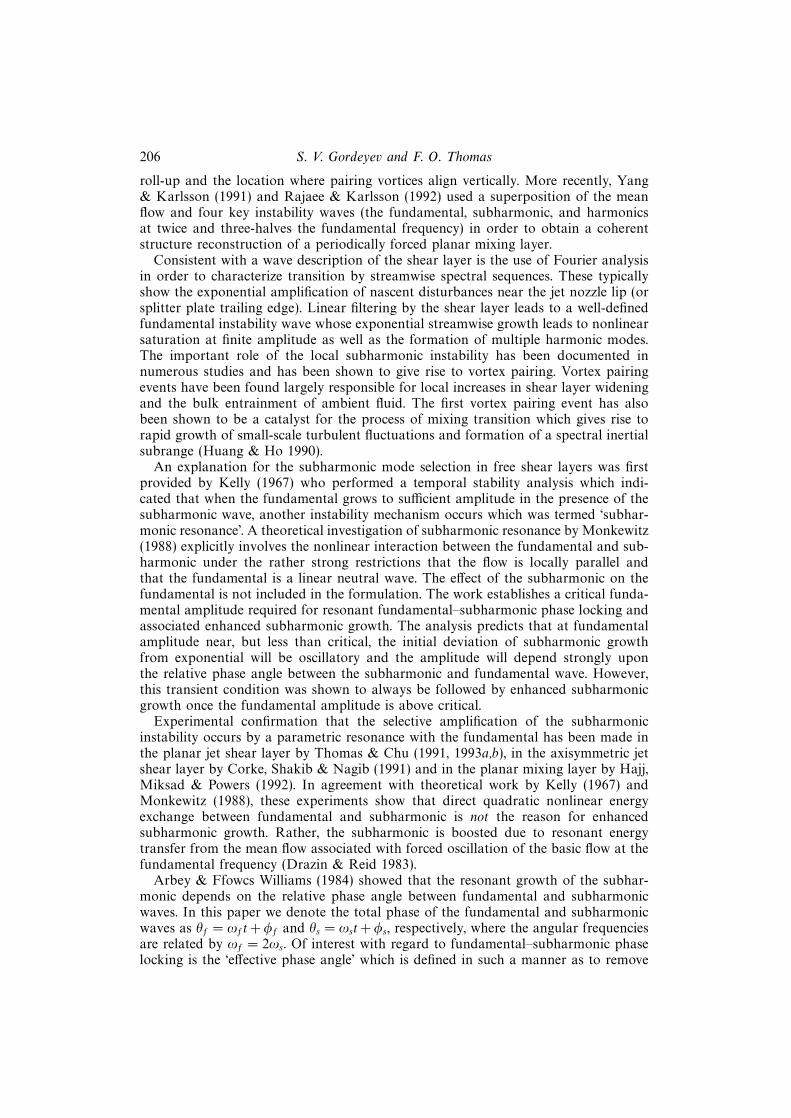
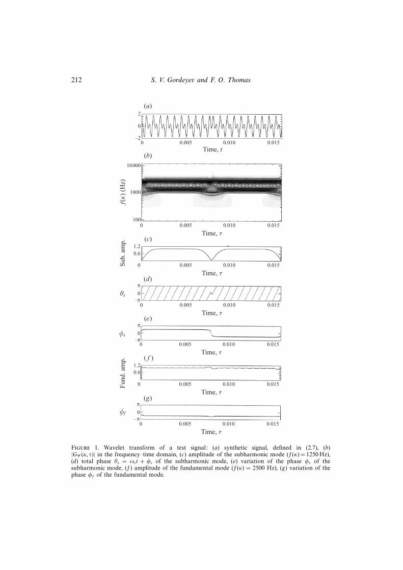
Since the focus of this work is on the temporal aspects of free shear layer transition,particularly those associated with time-dependent amplitude and phase behaviour ofthe subharmonic, standard Fourier analysis techniques will not suffice. Fourier analysisfails to track any temporal variation of signal amplitude and phase and could giverise to false results. In order to demonstrate this, consider a simple periodic signalwhich consists of the fundamental mode as a sine wave and a subharmonic mode asa cosine wave with a step-changing phase over equal increments in time:
signal(t) = sin (2π× 2500× t) +
{cos (2π× 1250× t+ π/2), 0 < t 6 0.008
cos (2π× 1250× t− π/2), 0.008 < t 6 0.016.
(2.7)
Fourier transformation of this signal would give a sine wave expansion signal(t) =∑An sin (2πnt) with mean subharmonic phase φs = 0 which is a completely misleading
result, while the wavelet transformation described above would properly resolve thetemporal phase variation for each mode. Figure 1 presents the results of applying theMorlet wavelet transform (2.1) to this signal. The raw signal is shown in figure 1(a)while figure 1(b) presents the modulus of the transform |GΨ (κ, τ)| in the frequency–timedomain (f(κ), τ). The darkest regions correspond to the highest levels of the modulus.The presence of the two tones at the fundamental and subharmonic frequencies of2.5 kHz and 1.25 kHz is clearly observed. Note the finite frequency resolution ofwavelet transform. The time evolution of each tone can be revealed by applicationof (2.1) for a fixed f(κ). For example, the amplitude variation of the subharmonic isshown in figure 1(c). The total phase θs = ωst + φs variation with time is presentedin figure 1(d). The ωst term gives rise to the observed ‘sawtooth’ character which alsoobscures any possible variation of the φs term. However, since ωs is known, it ispossible to subtract the ωst term from θs and thereby investigate the time dependenceof φs. This result is presented in figure 1(e). Note that the correct subharmonic phasevalues of φs = π/2 and φs = −π/2 are indicated with a π-shift occurring at t = 0.008.This figure also shows the finite time resolution of the wavelet transform as evidencedby the finite time interval over which the φs shift occurs. The fundamental amplitudeand phase variations are shown in figure 1(f) and figure 1(g), respectively. Again,the wavelet transform gives the correct values for these quantities. In contrast to thesubharmonic tone, the fundamental amplitude and phase are nearly constant in time.
The above example serves to illustrate that due to its filter-like behaviour, waveletanalysis can resolve the evolution of each mode independently, provided that the
212 S. V. Gordeyev and F. O. Thomas
2
0
–20 0.005 0.0150.010
(a)
Time, t(b)
10000
100
1000
0 0.005 0.0150.010
Time, τ
f(j)
(H
z)
0 0.005 0.0150.010
Time, τ
0 0.005 0.0150.010
Time, τ
0 0.005 0.0150.010
Time, τ
0 0.005 0.0150.010
Time, τ
0 0.005 0.0150.010
Time, τ
(c)
(d)
(e)
( f )
(g)
1.20.6
0
p
–p
0
p
–p
1.20.6
0
p
–p
Sub
. am
p.
hs
φs
Fun
d. a
mp.
φf
Figure 1. Wavelet transform of a test signal: (a) synthetic signal, defined in (2.7), (b)|GΨ (κ, τ)| in the frequency–time domain, (c) amplitude of the subharmonic mode (f(κ) = 1250 Hz),(d) total phase θs = ωst + φs of the subharmonic mode, (e) variation of the phase φs of thesubharmonic mode, (f) amplitude of the fundamental mode (f(κ) = 2500 Hz), (g) variation of thephase φf of the fundamental mode.

Temporal subharmonic amplitude and phase behaviour in a jet shear layer 213
frequency difference between modes is larger than the half-amplitude bandwidth ∆fA.Later this approach will be applied to the investigation of the φ phase variation of jetshear layer instability modes. This is possible since very low-amplitude acoustic exci-tation is applied near the most unstable shear layer frequency. Hence the fundamentaland subharmonic frequencies ωf and ωs are known a priori.
The fundamental and subharmonic instability frequencies in the jet shear layerunder investigation here occur at 2.5 kHz and 1.25 kHz as in the synthetic signal justconsidered. However, the fundamental and subharmonic bandwidths in the jet willbe wider than in the synthetic signal. Further, in the real flow additional instabilitymodes can be present that could potentially complicate application of the wavelettransform. Depending on the bandwidth of the wavelet transform at a given scale, it iscertainly possible to obtain ambiguous amplitude and phase results if multiple modesare present. In the Morlet wavelet transform used in our study, the bandwidth may beadjusted through the parameter b in equation (2.2). As long as the frequency spacingbetween spectral modes is greater than the bandwidth of the wavelet transform, thespectral peaks can be independently resolved. Jet shear layer streamwise velocityfluctuation power spectra as obtained over a wide range streamwise locations exhibitwell-defined spectral peaks at the fundamental and subharmonic frequencies (Thomas& Chu 1993a,b). Further, there are no other organized modes present within thespectral window of interest. Comparison of the measured power spectra to the half-amplitude bandwidths for the wavelet analysis corresponding to the values of b used inour study indicate that this requirement is satisfied in our case. This demonstrates thatthe wavelet analysis can resolve the fundamental and subharmonic modes properly.
The wavelet transformation is a natural generalization of the spectral transform-ation concept with Ψ (x) = exp (ix) a Fourier transformation. From (2.1), the wavelettransformation does not require integration over an infinite time domain centred ontime t = τ. Instead, integration is over a time interval proportional to T ≈ O(1/κ) =O(b/2πf(κ)) because of a Gaussian decay of Ψ (x) outside the domain. Note that Tis a function of the scale and thus provides a self-adjusting variable time window fordifferent scales. This demonstrates that the wavelet transformation provides short-time-average amplitude and phase information (on the order of T ) regarding thefunction g(t) at the moment t = τ for any unsteady signal. The price that one paysfor this time localization capability is the finite frequency or scale resolution of thesignal.
It should be pointed out that other techniques are available for recovering unsteadyamplitude and phase modulations. A technique intimately related to the wavelettransform is the Windowed Fourier Transform (WFT). A comparative example usingboth the Morlet wavelet transform and WFT to analyse jet shear layer hot-wire signalswill be presented in § 4. In addition, the complex digital demodulation technique (Kim,Khadra & Powers 1980) provides unsteady amplitude A(t) and total phase θ(t) if thesignal possesses a well-defined carrier frequency ω. Use of the Hilbert transform(Bendat & Piersol 1986) provides another option requiring only that the signal beof the form, signal(t) = A(t) exp (iθ(t)) so that the temporal frequency is calculatedas f(t) = 1/(2π) dθ/dt. However, each method has limitations in the sense that apriori knowledge of some aspect of the signal’s character is required. In contrast,the wavelet transformation provides a more general approach to investigating theirtransient character. Further, by the selection of different wavelet mother functions,one can highlight different aspects of the signal under investigation. That the motherfunction can be customized to highlight particular aspects of a signal is a realadvantage of wavelet analysis.

214 S. V. Gordeyev and F. O. Thomas
In practice equation (2.1) is commonly replaced by a finite discretized analogue,which is simply a numerical integral approximation for the case of a zero-orderinterpolation between data points:
GΨ (κ, τ) = κ
N∑i=1
giΨ∗(κ(ti − τ))∆ti. (2.8)
The signal gi is measured at discrete time points ti, i = 1...N with ∆ti = ti+1 − ti =∆t = const. Higher-order interpolation schemes can be used to improve accuracy. Thetheory of frames bounds the errors of the discrete wavelet calculations (Daubechies1992; Kaiser 1994) which can be large for very coarse discretization. We find thatin our case this computational error never exceeds 0.1%. In particular, for theMorlet wavelet it follows from investigation of equation (2.6) that the maximumresolution is κmax = π/((b+ 3)∆t) so that the maximum correctly resolved frequencyis fmax = b/((b+ 3)∆t). Consequently, in the case of the Morlet wavelet, the samplingfrequency should be at least (2(b + 3))/b times higher than the maximum frequencyto be resolved. Obviously, κmin is on the order of 1/T , where T is the total samplingtime.
3. The flow field facilityThe experiments were performed in the developing shear layer of a planar jet flow
field facility at the Hessert Center for Aerospace Research located at the Universityof Notre Dame. This is the same facility described in Thomas & Chu (1993a, b) andtherefore only a brief description of essential flow parameters will be presented here.
The two-dimensional nozzle is based upon a cubic contour with zero-derivative endconditions and has a contraction ratio of 16 : 1, ending in a slot exit that is D = 1.27 cmin width and H = 45.7 cm in height (i.e. aspect ratio = 36). A duct connecting theplenum chamber to the nozzle assembly contains acoustic baffling, honeycomb flowstraighteners and multiple turbulence reduction screens. The measurements wereperformed at a Reynolds number (based upon exit mean velocity, U0, and nozzle slotwidth, D) of approximately ReD = 1.7 × 10⁴ which corresponds to an exit velocityof U0 = 20.7 m s−1. The exit longitudinal turbulence intensity as measured on the jetcentreline is less than 0.04%. The jet initial mean velocity profiles are flat (i.e. ‘top-hat’shape) and the mean velocity variation across the nascent jet shear layers is closelyapproximated by a hyperbolic tangent type of profile. The free shear layers at thenozzle lip are both laminar and have an initial momentum thickness θ0 = 0.14 mm.
In order to facilitate control of the initial instability in frequency and amplitude,a loudspeaker was mounted in the duct upstream of the nozzle assembly. Two typesof excitation were used. The first involved bimodal forcing at the fundamental andsubharmonic frequencies in which case the signal to the loudspeaker was of formAf cos (2πfet)+As cos (πfet−φin/2). In this manner the exit perturbation amplitudes ofthe fundamental and subharmonic could be individually controlled as was the initialeffective phase angle, φin. The fundamental excitation frequency was always fe =2.5 kHz which is very near the most unstable shear layer frequency and corresponds toa Strouhal number based on exit momentum thickness of Stθ = 0.017. Measurementsmade with bimodal forcing allow comparison with results from works cited in theintroduction and also provide the framework for a main focus of this study which isthe temporal aspects of the naturally occurring subharmonic.
In the second type of experiment only the fundamental instability was artificially
Temporal subharmonic amplitude and phase behaviour in a jet shear layer 215
excited. No attempt was made to force the subharmonic instability, which developednaturally. For these experiments, the exit fluctuation intensity within a narrow fre-quency band centred on the fundamental frequency ranged from high to very lowlevels: 0.002% 6 (u2(fe))
1/2/U0 6 0.1%. Note that this range extends two orders ofmagnitude lower than the forcing levels used in the studies listed in table 1. Forthe lowest excitation amplitudes, the initial disturbance level was extremely smalland the shear layer inflectional instability mechanism provided ‘natural’ streamwiseamplification.
Constant-temperature anemometers were used in conjunction with conventional straight wire probes to acquire the u′(t) time series signals required for the Fourier andwavelet analysis. A laboratory PC was used for the digital data acquisition and fortraverse system control. The digital time-series data was sampled at 10 kHz and wasoff-loaded to a Sun Sparc 10 station for post processing.
In this paper x denotes the streamwise spatial coordinate measured from the nozzleexit plane while y is the cross-stream spatial coordinate whose origin is located at thecentre of the jet shear layer (i.e. U(y)/U0 = 0.5). Unless otherwise noted, the lateralmeasurement location corresponds to a position in the shear layer for which thelocal subharmonic wave amplitude is maximum. The measurements were performedat streamwise x locations extending from the jet lip to downstream of subharmonicsaturation (i.e. well upstream of the tip of jet potential core).
4. Experimental resultsWhen the continuous Morlet wavelet transform as described in § 2 was applied
to streamwise velocity fluctuation time series in the transitioning planar jet shearlayer, an interesting and previously unreported temporal behaviour of the naturalsubharmonic instability was observed that we next describe. By the term ‘naturalsubharmonic’ we imply that only the fundamental instability was artificially excitedat very low amplitude (u2(fe))
1/2/U0 ≡ u′f = 0.01% with no artificial excitation ofthe subharmonic instability used so that it develops naturally in the flow. Deferringpresentation of details pertinent to the measurement to later in § 4, for now we simplyrefer the reader to figure 2 for the purpose of illustrating a representative sample ofthis temporal subharmonic behaviour as derived from the wavelet analysis. This figurepresents the time evolution of subharmonic amplitude, subharmonic phase φs, andthe effective phase φeff , and shows the existence of two steady values of subharmonicphase φs with intermittent π-jumps between them. Note that these jumps are wellcorrelated with local drops in the subharmonic amplitude. This aspect is highlightedin figure 2 for one of the subharmonic phase-shift events. In contrast, time intervalsof stable subharmonic phase are associated with elevated subharmonic amplitude.This behaviour is unique to the subharmonic instability; the fundamental exhibitedcomparatively stable amplitude and phase.
As noted earlier, a technique that is closely related to the wavelet transform isthe Windowed Fourier Transform (WFT). However, the WFT provides only averagevalues of amplitude and phase of the mode over the data block size. Furthermore theblock size is fixed for all frequencies and the averaging over it leads to the possibilityof concealing temporal variations of the amplitude and phase that occur on timescales shorter than the block size. Obviously what one sees will then depend on thewindow length and proper adjustment of the block size can require considerable priorknowledge of the signal. In contrast, in § 2 it was shown that the wavelet transformutilizes a variable time-window approach, which allows one to recover the dynamics

216 S. V. Gordeyev and F. O. Thomas
τ (s)
–p/2
Sub
. am
p.(m
s–1
)φ
s (r
ad)
2.52.01.51.00.5
0 0.1 0.2 0.3
–p
0
p/2
p
0 0.1 0.2 0.3
τ (s)
2.5
2.0
1.5
1.0
0.5
0Sub
. am
p. (
m s
–1)
0.15 0.17 0.18 0.19 0.200.16
τ (s)
0.15 0.17 0.18 0.19 0.200.16τ (s)
–p/2
–p
0
p/2
p
φs (r
ad)
2p
3p/2p
p/2
00 0.1 0.2 0.3
τ (s)
φef
f (r
ad)
Figure 2. Temporal variation of subharmonic amplitude, phase and effective phase: u′f = 0.002%,
u′s = 0, x/θ0 = 110.
of the signal at any frequency with minimal prior knowledge about the signal onehas properly sampled. For example the temporal amplitude and phase behaviour ofthe subharmonic mode shown in figure 2 was found by direct application of theMorlet wavelet transform. However as shown in figure 3, with prior knowledge ofthe time scales involved in the dynamics as gleaned from wavelet analysis, the WFTis capable of showing the same essential characteristics, albeit less clearly. Actually,these drawbacks of the WFT led to the development of the wavelet transform. Anexcellent discussion highlighting both the similarities and key differences about theWFT and the continuous wavelet transform can be found in §§ 2 and 3, respectively

Temporal subharmonic amplitude and phase behaviour in a jet shear layer 217
t (s)
Fun
d. a
mp.
(m s
–1)
2.52.01.51.00.5
0 0.05 0.10 0.15VFT
2.52.01.51.00.5
0 0.05 0.10 0.15
Windowed Fourier transform Wavelet transform
0 0.05 0.10 0.15
VFT
0 0.05 0.10 0.15
0 0.05 0.10 0.15VFT
0 0.05 0.10 0.15
0 0.05 0.10 0.15VFT
0 0.05 0.10 0.15
Sub
. am
p.(m
s–1
)
2.52.01.51.00.5
p
–p/20
–p
φf (
rad) p/2
p
–p/20
–p
φs (
rad) p/2
p
–p/20
–p
p/2
2.52.01.51.00.5
p
–p/20
–p
p/2
t (s)
Figure 3. Comparison between windowed Fourier and wavelet transforms.
of Kaiser (1994). Also shown in figure 3 are the values of subharmonic amplitudeand phase provided by conventional Fourier transform analysis (designated by FT).
A systematic series of experiments was undertaken in an effort to (i) determine thelocations and initial conditions for which temporal subharmonic behaviour like thatshown in figure 2 occurs, (ii) relate these effects to the previously cited studies whichuse conventional Fourier analysis techniques. In the following portions of this sectionresults from two types of experiments are presented. Consideration is first given tothe case of bimodal forcing at the fundamental and subharmonic frequencies over awide range of initial F–S phase angles. The forcing amplitudes for these experimentsare similar to those used in the investigations reviewed in § 1. The purpose of theseexperiments is to provide a basis for comparison with previous work and to set theframework for contrasting with results involving the natural subharmonic shear layerevolution. For these measurements we utilize experimental methods similar to thoseused in the cited literature in addition to the wavelet analysis technique.
It is the natural subharmonic evolution that forms the focus of the second group ofexperiments. For these, only the fundamental instability is excited at low amplitudewhile the subharmonic is allowed to develop naturally. The shear layer dynamicsobserved in these experiments are characterized by an inherent temporal variationthat forms a major focus of this work. The observed temporal behaviour of thesubharmonic instability is the motivation for a Hamiltonian system approach tovortex pairing and tearing interactions in the shear layer. However, it will be later

218 S. V. Gordeyev and F. O. Thomas
2.0
1.5
1.0
0.5
0–15 –10 –5 0 5 10 15
fE
fE/2
Mod
al a
mp.
(m
s–1
)
p
p/2
0
–p/2
–p–15 –10 –5 0 5 10 15
φef
f (r
ad)
y /h0
Figure 4. Measured cross-stream variation of fundamental and subharmonic amplitudes and localeffective phase at x/θ0 = 60 for φin = 180◦.
shown that the resulting model also predicts many aspects observed in the experimentsusing bimodal forcing at higher amplitude.
Measurements were performed at several lateral locations within the jet shear layer.However, since a focus of our paper is on the dynamic behaviour of the subharmonicinstability, the data that we present below were obtained near the location of maximumsubharmonic amplitude. These may be considered representative of results obtainedat the other lateral locations, which exhibited qualitatively similar dynamic behaviour.
4.1. Bimodal forcing experiments
In experiments using bimodal forcing at fundamental and subharmonic frequencies,several amplitude combinations were explored. In this section we will present resultsobtained for two of these combinations that are representative of the type of behaviourencountered and which serve to provide a basis for comparison with previous studies.In the first case (u2(fe))
1/2/U0 ≡ u′f = 0.01% and (u2(fe/2))1/2/U0 ≡ u′s = 0.1%. In thesecond case both fundamental and subharmonic forcing amplitudes were the same:u′f = u′s = 0.1%. The fairly high level of excitation used in these experiments modifiesthe shear layer dynamics in the sense that it reduces the natural ‘phase jitter’ andallows the use of standard Fourier analysis techniques for investigating the spatialamplitude and phase behaviour of the developing modes.
In terms of tracking the streamwise evolution of the effective F–S phase anglecare must be taken in the selection of the lateral location of the measurement. Asan example, figure 4 shows a typical cross-stream profile of the fundamental andsubharmonic modal amplitudes as well as the local effective F–S phase angle φeff
obtained at the x/θ0 = 60 location for the initial effective phase φin = 180◦. It isapparent from this figure (and other cross-stream profiles that were obtained but are
Temporal subharmonic amplitude and phase behaviour in a jet shear layer 219
p
p/2
0
–p/2
–p
φef
f (r
ad)
p
p/2
0
–p/2
–p
φef
f (r
ad)
p
p/2
0
–p/2
–p
φef
f (r
ad)
1.00
0.75
0.50
0.25A/A
max
p
0 80 160 320240
φin (deg.)0 80 160 320240
φin (deg.)
0 80 160 320240 0 80 160 320240
0 80 160 320240 0 80 160 320240
1.00
0.75
0.50
0.25A/A
max
1.00
0.75
0.50
0.25A/A
max
(a) (b)x /h0 =50
x /h0 =60
x /h0 =80
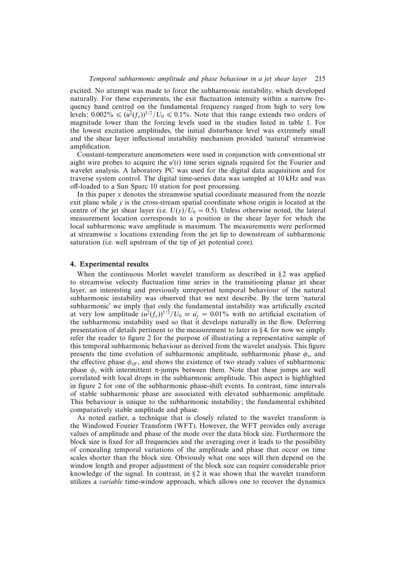
Figure 5. (a) Local subharmonic amplitude variation and (b) local effective phase as a function ofφin for u′f = 0.01%, u′s = 0.1%.
not presented) that the local φeff value strongly depends on the cross-stream locationin the shear layer. For this reason, care must be exercised when comparing effectivephase results from different experiments. It should also be remembered that the initialeffective phase, φin, is actually a value imposed at the exit plane of the jet nozzle.Due to the strong lateral spatial gradients in φeff , the corresponding initial value inthe shear layer will vary accordingly.
In order to demonstrate the local response of subharmonic amplitude to initialF–S phase angle, φin, figure 5(a) presents measurements of subharmonic amplitude(normalized by the local subharmonic maximum) as obtained at selected x/θ0 lo-cations both upstream and near subharmonic mode saturation as a function of theinitial effective phase angle, φin. Figure 5(b) presents the corresponding local valuesof effective F–S phase angle, φeff , as a function of φin. The data of figures 5(a) and5(b) correspond to fundamental and subharmonic forcing amplitudes of u′f = 0.01%and u′s = 0.1%.
Figure 5(a) shows that at x/θ0 = 50 the subharmonic amplitude exhibits a cleardependence on the initial effective phase angle, with a maximum near φin = 30◦and a minimum for φin = 220◦. Similar subharmonic amplitude behaviour can beobserved at the x/θ0 = 60 station with the local subharmonic amplitude maximumat φin ≈ 40◦ and minimum amplitude shifted to φin ≈ 260◦. By x/θ0 = 80 (which isnear subharmonic amplitude saturation) there exists a broad range of initial effectivephase angles for which the subharmonic amplitude remains virtually constant andvery near the maximum value. These values of φin are associated with vortex pairing.Only for a limited range of φin does the subharmonic amplitude decrease. There is a

220 S. V. Gordeyev and F. O. Thomas
cusp centred near φin = 280◦ in which the subharmonic amplitude drops drastically.The cusp of reduced subharmonic amplitude (which is associated with vortex tearing)is quite localized in φin. This result demonstrates that in the nonlinear region of theflow, vortex pairing is highly favoured (i.e. most φin values will favour vortex pairing).The behaviour shown for x/θ0 = 80 is very reminiscent of that shown in figure 3(c)of Husain & Hussain (1995). They observed a cusp at φin = 216◦ for higher forcinglevels (both fundamental and subharmonic were excited at 0.1%). Their experimentsat a forcing level of 1% showed similar behaviour with the cusp occurring at 306◦.
Figure 5(b) shows the average local effective phase angle φeff as a function of φinfor the same streamwise stations as those presented in figure 5(a). At the x/θ0 = 50location the local effective phase varies linearly with φin. At x/θ0 = 60 the variationof φeff with φin is observed to be quite nonlinear for 0◦ < φin < 120◦ and 240◦ < φin <360◦. Finally, near x/θ0 = 80 the effective phase exhibits a strong nonlinear variationwith φin. In particular, the local effective phase only weakly follows the φin linearvariation and appears to lock onto either one of two values. There are two localizedπ-phase shifts between these phase plateaux for φin ≈ 0◦ and φin ≈ 270◦. The lattervalue is centred near the cusp corresponding to minimum subharmonic amplitudeshown in figure 5(a). Figure 5(b) shows that once F–S locking occurs, there are twoallowed effective F–S phase angles. These are shifted by π radians with respect toeach other and the values are observed to be largely independent of φin (though theyare functions of x/θ0).
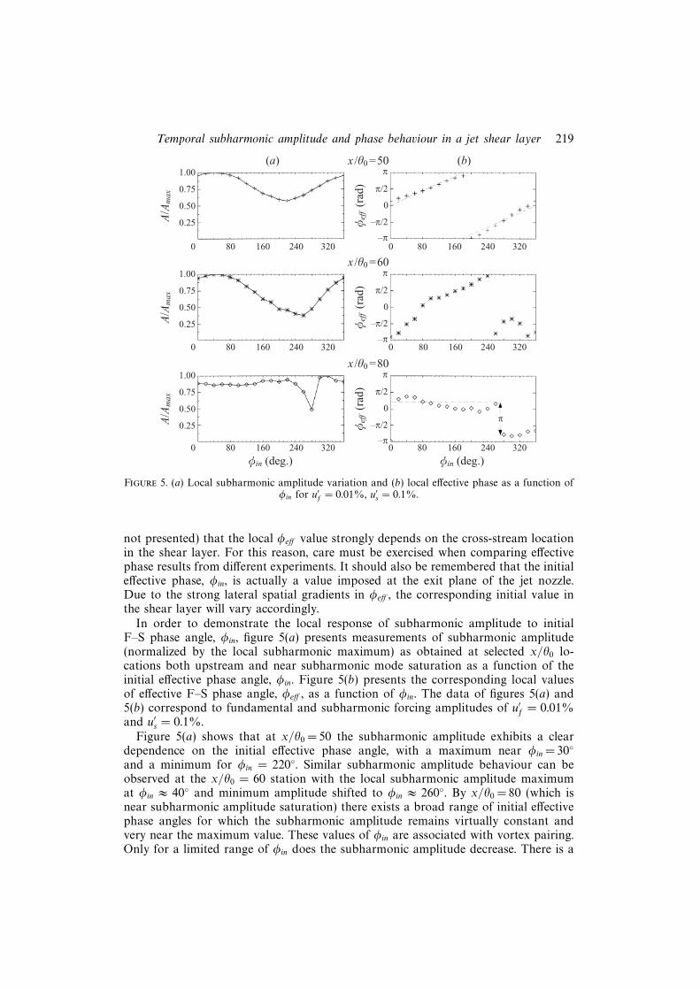
For the bimodal shear layer excitation condition corresponding to figure 5(a,b),two values of φin were selected in order to investigate the streamwise subharmonicevolution. The selected values were φin = 0◦ which corresponds to strong subharmonicgrowth (i.e. vortex pairing) and φin = 260◦ which corresponds to subharmonic sup-pression (i.e. vortex tearing). The streamwise evolution of modal amplitudes of boththe fundamental instability, fe, and subharmonic, fe/2 for both φin cases are shownin figure 6 (as determined from conventional Fourier analysis). The profound effectthat the initial F–S phase angle φin can have upon the development of the jet shearlayer is apparent from this figure. In the φin = 0◦ case, the subharmonic exhibitsstrong growth and saturates near x/θ0 = 80. In the φin = 260◦ case the subharmonicamplitude is strongly suppressed over the range 60 < x/θ0 < 120 and is actually indecay over 55 < x/θ0 < 80. The back effect of the subharmonic on the fundamental isalso apparent, an aspect not treated in the theory of Monkewitz (1988). Figure 6 alsopresents the streamwise variation in average effective phase φeff (also determined byFourier analysis) which behaves quite differently in each case. In both cases, however,the local effective phase angle φeff is observed to vary continuously with x. Thisindicates that the values of the effective phase φeff plateaux shown in figure 5(b)for x/θ0 ≈ 80 are local and will, in general, vary in the streamwise direction. Note,however, that in the region of subharmonic decay (55 < x/θ0 < 80) in figure 6, theeffective phase curves for the two cases are separated by π radians. The theoreticalmodel, to be presented in § 5, will explain the existence of the two possible values forthe local effective phase and the π-dislocation in phase separating the two. Figure 6indicates that while the particular value of φeff associated with the plateaux in phasevary in the streamwise direction, the local values associated with pairing and tearingremain separated by π radians in the region of strongest subharmonic suppression.
In the bimodal forcing experiments the Morlet wavelet transform was applied tothe experimentally obtained streamwise velocity fluctuation time histories. The phasetime histories φf(t) and φs(t) were extracted by application of equation (2.1) at theappropriate fixed κ. The associated effective phase time history was then obtained
Temporal subharmonic amplitude and phase behaviour in a jet shear layer 221
p
p/2
0
–p/2
–p
φef
f (ra
d)
(a)
(b)
x /h0
0.8
0.6
0.4
0.2
0 20 40 60 80 100 120 140
φin = 0°φin = 260°
2.52.01.51.00.5
0 20 40 60 80 100 120 140
(c)
0 20 40 60 80 100 120 140
(d )
0 20 40 60 80 100 120 140
φin = 0°φin = 260°
φin = 0°φin = 260°
φin = 0°φin = 260°
p
r.m.s
. φef
f
2.0
1.5
1.0
0.5
Sub
. am
p. (
m s
–1)
Fun
d. a
mp.
(m
s–1
)
Figure 6. Streamwise evolution of fundamental amplitude, subharmonic amplitude, φeff and r.m.s.of φeff for φin = 0◦ (pairing) and φin = 260◦ (tearing), u′f = 0.01%, u′s = 0.1%.
as φeff (t) = φf(t) − 2φs(t). The root-mean-square (r.m.s.) value of the φeff (t) timehistory provides an indication of regions where temporal phase variations are mostsignificant. The lowest plot of figure 6 presents the resulting streamwise variationof the r.m.s. of the effective phase as determined from the wavelet analysis. Thisprovides a measure of the degree of temporal variation of the measured effective F–Sphase φeff . As shown in the example presented in figure 1, the finite time resolutionof the wavelet transform will have the tendency to smooth a sudden shift in phase.In effect, the step change in phase is low-pass filtered. As such, one could argueregarding the physical relevance of the r.m.s. value of the effective phase. However,there is no question that it represents a good indicator of those x locations whereφeff exhibits temporal variation and this is our only purpose in presenting the r.m.s.phase values shown in figure 6. The streamwise variation in r.m.s. is presented forboth excitation cases. In the case φin = 0◦, which favours strong subharmonic growth(i.e. vortex pairing) the r.m.s. ≈ 0 for all x indicating the inherent temporal stability

222 S. V. Gordeyev and F. O. Thomas
p
p/2
0
–p/2
–p
φef
f (ra
d)
(a)
(b)
x /h0
0.80.6
0.40.2
0 20 40 60 80 100 120 140
2.52.01.51.00.5
0 20 40 60 80 100 120 140
(c)
0 20 40 60 80 100 120 140
(d )
0 20 40 60 80 100 120 140
p
r.m.s
. φef
f
2.0
1.5
1.0
0.5
Sub
. am
p. (
m s
–1)
Fun
d. a
mp.
(m
s–1
)
1.0
φin =160°φin =180°
φin =160°φin =180°
φin =160°φin =180°
φin =160°φin =180°
Figure 7. Streamwise evolution of fundamental amplitude, subharmonic amplitude, φeff and r.m.s.of φeff for φin = 160◦ (pairing) and φin = 180◦ (tearing), u′f = u′s = 0.1%.
of the local effective F–S phase. In the second case, φin = 260◦, which corresponds tosubharmonic suppression (i.e. vortex tearing), the r.m.s. is observed to be significantlyincreased for 60 < x/θ0 < 120 which is the same streamwise region which exhibitssubharmonic suppression. This implies that this region is also characterized by a highlevel of temporal variation in phase. We will consider this region further when wepresent additional wavelet analysis results in the next section.
Figure 7 presents the streamwise amplitude variation of the fundamental andsubharmonic modes, the local effective F–S phase (as determined by Fourier analysis)and the r.m.s. of the effective phase (obtained via wavelet analysis as described above)for bimodal excitation at amplitudes u′f = u′s = 0.1%. Two cases are shown: φin = 160◦and φin = 180◦. Due to the higher fundamental excitation amplitude, the fundamentalsaturates at x/θ0 ≈ 35 in both cases which is well upstream of the saturation locationshown in figure 6. Again, significant disparities in the streamwise evolution of thesubharmonic instability may be observed. In particular, the subharmonic is suppressedin the region 40 < x/θ0 < 70 for the φin = 180◦ case. In contrast, the φin = 160◦

Temporal subharmonic amplitude and phase behaviour in a jet shear layer 223
3.14
1.57
0
–1.57
–3.140 0.5 1.0 1.5
x/xs
Fund. amplitudeSub. amplitude
Eff. phase for u′f =
0.006%0.01%0.02%0.06%0.1%
Increasing u′f
Figure 8. Streamwise evolution of fundamental amplitude, natural subharmonic amplitude andφeff for several u′f; u′s = 0 in each case.
case is characterized by strong subharmonic growth. As in figure 6, there is a πdifference in local φeff values between the two cases in the region 40 < x/θ0 < 50which is associated with strong subharmonic suppression. Note, also that for theφin = 180◦ case, the r.m.s. exhibits elevated values in this region as was the casein figure 6. In contrast, the φin = 160◦ case shows values of r.m.s. ≈ 0 indicatinglittle temporal variation in effective phase. This leads to the conclusion that thesubharmonic suppression is characterized by an inherently unsteady effective phasebehaviour. Comparison of figures 6 and 7 also indicates that the φin giving rise tosubharmonic suppression is clearly dependent upon the initial excitation level.
4.2. Single mode forcing experiments: natural subharmonic evolution
In the second series of experiments, only the fundamental instability wave wasartificially excited. Since there is no artificial forcing at the subharmonic frequency,the subharmonic mode will develop naturally and eventually reach an optimum phaserelationship with the fundamental mode. These experiments focus on the naturalaspects of the F–S interaction which will be shown to be inherently unsteady. Bothstandard Fourier and the Morlet wavelet transformations were applied in order toprocess the hot-wire signals.
In figure 8 the streamwise evolution of both fundamental and subharmonic modesas well as the local average effective phase angle φeff are presented for several differentfundamental excitation amplitudes spanning two orders of magnitude: 0.006% < u′f <0.1%. The subharmonic is not artificially excited; u′s = 0. There will, of course, be anaturally occurring subharmonic perturbation near the nozzle lip due to upstreamfeedback. The streamwise coordinate x is non-dimensionalized by xs which is thelocation of subharmonic mode saturation for each case. All measurements weretaken along the line of the local subharmonic cross-stream maxima. Standard Fourier
224 S. V. Gordeyev and F. O. Thomas
analysis techniques were utilized to obtain the modal amplitudes and average localeffective phase shown in figure 8.
In the initial region x/xs < 0.5, a wide range of φeff values is observed and theseclearly depend on fundamental excitation level. The fundamental wave amplitudesaturates farther upstream with increased initial excitation amplitude, u′f , as indicated.However, for x/xs > 0.5, the local effective phase angles are found to converge and allexhibit a similar streamwise variation. In this region the fundamental mode decays,the subharmonic mode is strongly amplified and all φeff values remain near a value of3π/4 ≈ 2.4. Note that this is quite near the local values of φeff which were found to beassociated with strong subharmonic amplification in the bimodal forcing experiments(figures 6 and 7) In fact, there is a strong similarity in the streamwise variation inφeff observed in figures 8, 7 and 6. Figure 8 shows that just upstream of subharmonicmode saturation the fundamental reaches minimum amplitude and φeff exhibits asudden drop to a value near zero.
The data of figure 8 were used to determine whether a critical fundamentalamplitude exists for onset of F–S resonance. The criterion used to characterizeinitiation of resonance was the departure of the local effective phase φeff from itsinitial streamwise variation and its approach toward the converged effective phasevalues shown in figure 8. With the exception of the highest excitation case, thefundamental amplitudes corresponding to these streamwise locations were found tobe at a value of 0.016U0 within experimental uncertainty. This corresponds well tothe value of 0.015U0 predicted by the analysis of Monkewitz (1988) for a mixing layerwith velocity ratio R = 1.
These results show that for a wide range of initial fundamental excitation amplitudesthe shear layer will, after the fundamental reaches sufficient amplitude (approximately0.016U0), begin to exhibit a similar nonlinear variation of φeff as a function ofx/xs. In a sense, with sufficient downstream distance the effect of initial conditionsis gradually lost and a common phase and subharmonic amplitude behaviour isobserved. Sustained vortex tearing must be artificially forced via bimodal excitationand is not observed in the results depicted in figure 8. From figure 8 one can alsoconclude that φeff at x = 0 is a function of initial fundamental excitation amplitudeand therefore there is no unique optimum φin value for the jet shear layer. An amplitudedependence of φin for subharmonic suppression was also noted in the bimodal forcingexperiments.
Two cases of low-level fundamental excitation were selected in order to investigatethe temporal aspects of the F–S interaction. The streamwise variation of both the feand fe/2 modal amplitudes as well as the local average effective phase φeff and its r.m.s.are presented in figure 9 for the case of extremely low-level fundamental excitation,u′f = 0.002% (i.e. slightly above natural background disturbances within a narrowfrequency band centred on fe). It is apparent from the high values of r.m.s. that theeffective phase exhibits a high degree of temporal unsteadiness, especially in the regionextending to x/θ0 ≈ 80. In the region x/θ0 > 80 the temporal φeff -fluctuations aresignificantly reduced. This indicates that the fundamental and natural subharmonicmode establish a certain degree of resonant phase locking in this region. This isconfirmed by the streamwise variation in the cross-bicoherence which is presentedin figure 9. Note the large increase in cross-bicoherence b2(fe,−fe/2) commencingnear x/θ0 ≈ 80 which confirms the enhanced phase locking between the fundamentaland subharmonic waves at this location. However, even in the region of strongestsubharmonic growth, there is still an inherent unsteadiness and the r.m.s. remainsgreater than zero. This is also shown in the streamwise amplitude variation of the

Temporal subharmonic amplitude and phase behaviour in a jet shear layer 225
p
p/2
0
–p/2–p
φef
f (ra
d)
x /h0
0.8
0.6
0.4
0.2
0 20 40 60 80 100 120 140
0.6
0.4
0.2
0 20 40 60 80 100 120 140
0 20 40 60 80 100 120 140
r.m.s
. φef
f 2.0
1.5
1.0
0.5
Sub
. am
p. (
m s
–1)
Fun
d. a
mp.
(m
s–1
)
0 20 40 60 80 100 120 140
0 20 40 60 80 100 120 140
1.00.80.60.40.2
b2(f
e, –
f e/2
)
Figure 9. Streamwise variation of fundamental and subharmonic amplitudes, φeff , r.m.s. of φeff
and cross-bicoherence for u′f = 0.002%, u′s = 0.
subharmonic which appears quite jagged. The amplitude was computed by standardFourier analysis with an ensemble average over twenty five data blocks. Due to theinherent temporal variation of the natural subharmonic this was insufficient in thiscase to achieve a smooth spectral estimate. This behaviour may be contrasted withthe case of moderate fundamental excitation u′f = 0.01%, u′s = 0 which is presentedin figure 10. In this case the subharmonic amplitude reaches a much higher saturationvalue and the spectral estimates are smooth. The corresponding r.m.s. values arenear zero which indicates a smaller degree of the temporal phase variation. Thisindicates that the F–S phase locking is much stronger in this case and the increasedamplification of the subharmonic results.

226 S. V. Gordeyev and F. O. Thomas
p
p/2
0
–p/2
–p
φef
f (ra
d)
x /h0
0.80.6
0.40.2
0 20 40 60 80 100 120 140
2.0
1.5
1.0
0.5
0 20 40 60 80 100 120 140
0 20 40 60 80 100 120 140
0 20 40 60 80 100 120 140
r.m.s
. φef
f
2.0
1.5
1.0
0.5
Sub
. am
p. (
m s
–1)
Fun
d. a
mp.
(m
s–1
)
1.0
Figure 10. Streamwise variation of fundamental and subharmonic amplitudes, φeff and r.m.s. ofφeff for u′f = 0.01%, u′s = 0.
The results presented to this point demonstrate that temporal variation in effectivephase behaviour (as evidenced by high r.m.s. values of effective phase) may be ex-pected in bimodal forcing experiments in those regions characterized by subharmonicmode suppression even if the forcing amplitudes are quite large. In addition, tem-poral phase variation is the rule in experiments involving low-amplitude forcing ofthe fundamental and natural development of the subharmonic. In order to properlyinvestigate these temporal aspects of the shear layer dynamics, a wavelet transfor-mation technique was applied in the analysis of the hot-wire signals. To demonstratethe effectiveness of the wavelet transform for this purpose, consider the modulus ofthe Morlet wavelet transform of the shear layer hot-wire signal which is presented infigure 11. The signal for figure 11 corresponds to u′f = 0.002%, u′s = 0 (no artificialsubharmonic excitation) at x/θ0 = 90 (i.e. just upstream of subharmonic saturation,see figure 9). The abscissa is time τ(s) and the ordinate is f(κ) = bκ/2π (and is ex-pressed in Hz). The use of frequency units on the ordinate is potentially misleadingand it must be emphasized that this should not be interpreted as implying periodicity.

Temporal subharmonic amplitude and phase behaviour in a jet shear layer 227
10000
1000
1000 0.05 0.10 0.15
Sub.
Fund.
τ (s)
f(j)
(H
z)
Figure 11. Morlet wavelet transform modulus |GΨ (κ, τ)| at x/θ0 = 90, u′f = 0.002%, u′s = 0.
Rather this is a convenient way to relate an event from the wavelet analysis to thestandard Fourier analysis results. The modulus of the signal is plotted in the formof a shaded contour plot with darker shading associated with higher levels of thesignal modulus. The f(κ) values associated with the fundamental and subharmonicinstabilities are identified on the ordinate. The temporal variation of the subharmonicmodulus is especially apparent. The modulus of the fundamental is, by comparison,fairly constant. Maxima and minima of the subharmonic modulus do not appearcorrelated with any similar variation in the fundamental. Figure 11 clearly demon-strates the inherent temporal variation that characterizes the natural subharmonicinstability.
As in the example presented in figure 1, at any selected x-station one can obtaina time series corresponding to the amplitude envelope and phase of individual shearlayer modes by taking a ‘slice’ of the wavelet transform (e.g. like figure 11) at theappropriate f(κ). Since the focus of this paper is on the fundamental and subharmonicinstabilities, this manner of presenting the wavelet transformation results is moreappropriate than full contour plots in f(κ), τ space. Consequently, in the remainder ofthe paper wavelet results will be presented in terms of derived amplitude and phasetime series for the fundamental and subharmonic instability waves. Recall also thatit is the phase term φ and not θ that is of primary interest.
Figure 2 presented the time variation of the amplitude and phase of the subhar-monic instability at x/θ0 = 110 for the case of u′f = 0.002% and u′s = 0. Figure 9 showsthis location to be in a region of natural subharmonic growth although the r.m.s.of the effective phase > 0. Examination of figure 2 reveals an interesting temporalbehaviour of the subharmonic mode which was already highlighted at the beginningof this section. It shows the existence of two steady values of subharmonic phasewith intermittent π-jumps between them. These phase jumps are observed to be wellcorrelated with local drops in the subharmonic amplitude. In contrast, time intervalsof stable subharmonic phase are associated with elevated subharmonic amplitude.Although not presented in figure 2, the fundamental amplitude and phase do notshow any behaviour of this sort; both exhibit only very small temporal variation. Theπ-jumps in subharmonic phase give rise to corresponding intermittent disruptions inthe local effective phase angle, φeff , which is also presented in figure 2. The resonant
228 S. V. Gordeyev and F. O. Thomas
2.0
1.5
1.0
0.5
0 0.1 0.2 0.3Sub
. am
p. (
m s
–1)
0
0.1 0.2 0.3
0 0.1 0.2 0.3
p/2
p
3p/2
2p
p/2
p
τ (s)
0
–p/2
–p
φs (
rad)
φef
f (ra
d)
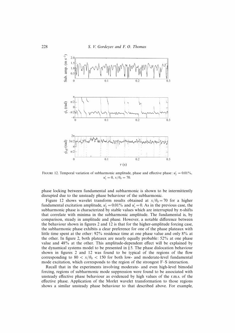
Figure 12. Temporal variation of subharmonic amplitude, phase and effective phase: u′f = 0.01%,
u′s = 0, x/θ0 = 70.
phase locking between fundamental and subharmonic is shown to be intermittentlydisrupted due to the unsteady phase behaviour of the subharmonic.
Figure 12 shows wavelet transform results obtained at x/θ0 = 70 for a higherfundamental excitation amplitude, u′f = 0.01% and u′s = 0. As in the previous case, thesubharmonic phase is characterized by stable values which are interrupted by π-shiftsthat correlate with minima in the subharmonic amplitude. The fundamental is, bycomparison, steady in amplitude and phase. However, a notable difference betweenthe behaviour shown in figures 2 and 12 is that for the higher-amplitude forcing case,the subharmonic phase exhibits a clear preference for one of the phase plateaux withlittle time spent at the other: 92% residence time at one phase value and only 8% atthe other. In figure 2, both plateaux are nearly equally probable: 52% at one phasevalue and 48% at the other. This amplitude-dependent effect will be explained bythe dynamical systems model to be presented in § 5. The phase dislocation behaviourshown in figures 2 and 12 was found to be typical of the regions of the flowcorresponding to 80 < x/θ0 < 150 for both low- and moderate-level fundamentalmode excitation, which corresponds to the region of the strongest F–S interaction.
Recall that in the experiments involving moderate- and even high-level bimodalforcing, regions of subharmonic mode suppression were found to be associated withunsteady effective phase behaviour as evidenced by high values of the r.m.s. of theeffective phase. Application of the Morlet wavelet transformation to those regionsshows a similar unsteady phase behaviour to that described above. For example,
Temporal subharmonic amplitude and phase behaviour in a jet shear layer 229
2.0
1.5
1.0
0.5
0 0.1 0.2 0.3Sub
. am
p. (
m s
–1)
0
0.1 0.2 0.3
0 0.1 0.2 0.3
p/2
p
3p/2
2p
p/2
p
τ (s)
0
–p/2
–p
φs (
rad)
φef
f (ra
d)
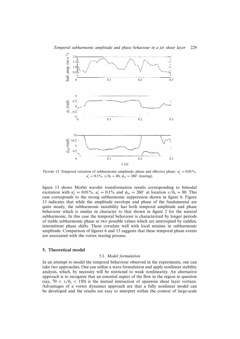
Figure 13. Temporal variation of subharmonic amplitude, phase and effective phase: u′f = 0.01%,
u′s = 0.1%, x/θ0 = 80, φin = 260◦ (tearing).
figure 13 shows Morlet wavelet transformation results corresponding to bimodalexcitation with u′f = 0.01%, u′s = 0.1% and φin = 260◦ at location x/θ0 = 80. Thiscase corresponds to the strong subharmonic suppression shown in figure 6. Figure13 indicates that while the amplitude envelope and phase of the fundamental arequite steady, the subharmonic instability has both temporal amplitude and phasebehaviour which is similar in character to that shown in figure 2 for the naturalsubharmonic. In this case the temporal behaviour is characterized by longer periodsof stable subharmonic phase at two possible values which are interrupted by sudden,intermittent phase shifts. These correlate well with local minima in subharmonicamplitude. Comparison of figures 6 and 13 suggests that these temporal phase eventsare associated with the vortex tearing process.
5. Theoretical model5.1. Model formulation
In an attempt to model the temporal behaviour observed in the experiments, one cantake two approaches. One can utilize a wave formulation and apply nonlinear stabilityanalysis, which, by necessity will be restricted to weak nonlinearity. An alternativeapproach is to recognize that an essential aspect of the flow in the region in question(say, 70 < x/θ0 < 150) is the mutual interaction of spanwise shear layer vortices.Advantages of a vortex dynamics approach are that a fully nonlinear model canbe developed and the results are easy to interpret within the context of large-scale
230 S. V. Gordeyev and F. O. Thomas
jth vortex (xj, yj)
y
x
kf =1
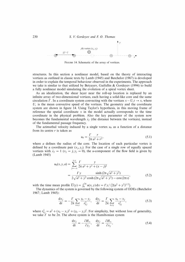
Figure 14. Schematic of the array of vortices.
structures. In this section a nonlinear model, based on the theory of interactingvortices as outlined in classic texts by Lamb (1945) and Batchelor (1967) is developedin order to explain the temporal behaviour observed in the experiments. The approachwe take is similar to that utilized by Betyayev, Gaifullin & Gordeyev (1994) to builda fully nonlinear model simulating the evolution of a spiral vortex sheet.
As an idealization, the shear layer near the roll-up location is replaced by aninfinite array of two-dimensional vortices, each having a solid-like core and the samecirculation Γ . In a coordinate system convecting with the vortices x−Uct→ x, whereUc is the mean convective speed of the vortices. The geometry and the coordinatesystem are shown in figure 14. Using Taylor’s hypothesis, in this moving frame ofreference the spatial coordinate x in the model actually corresponds to the timecoordinate in the physical problem. Also the key parameter of the system nowbecomes the fundamental wavelength λf (the distance between the vortices), insteadof the fundamental passage frequency.
The azimuthal velocity induced by a single vortex uθ as a function of a distancefrom its centre r is taken as
uθ =Γ
2π
r
a2 + r2, (5.1)
where a defines the radius of the core. The location of each particular vortex isdefined by a coordinate pair (xj, yj). For the case of a single row of equally spacedvortices with λf = 1 (xj = j, yj = 0), the u-component of the flow field is given by(Lamb 1945)
u0(x, y, a) =
+∞∑j=−∞
Γ
2π
y
a2 + y2 + (x− j)2
=Γy
2√a2 + y2
sinh (2π√a2 + y2)
cosh (2π√a2 + y2)− cos (2πx)
, (5.2)
with the time mean profile U(y) =∫ 2π
0u(x, y) dx = Γy/
(2(a2 + y2)1/2
).
The dynamics of the system is governed by the following system of ODEs (Batchelor1967; Lamb 1945):
dxjdt
= − Γ2π
∑k 6=j
yk − yjr2kj
,dyjdt
=Γ
2π
∑k 6=j
xk − xjr2kj
, (5.3)
where r2kj = a2 + (xk − xj)2 + (yk − yj)2. For simplicity, but without loss of generality,
we take Γ to be 2π. The above system is the Hamiltonian system
dxjdt
= −∂H∞∂yj
,dyjdt
=∂H∞∂xj
, (5.4)

Temporal subharmonic amplitude and phase behaviour in a jet shear layer 231
y
x
d
ε
1
Figure 15. The geometry of the perturbed vortex system.
with
H∞(xj, yj) = −1
2
∑j
∑k 6=j
log (r2kj). (5.5)
Consider, in particular, a line of vortices equally spaced along the x-axis with unitydistance between them (λf = 1) as shown in figure 15. Introduce a subharmonicperturbation with λs = 2λf = 2 as
xj = j + δ cos (2πj/λs), yj = ε cos (2πj/λs). (5.6)
Now the evolution of the system is characterized by the two new variables (δ(t), ε(t)).Formally the sum (5.5) does not exist for this system, but equals −∞. However, thisproblem is eliminated by subtracting the undisturbed H∞(j, 0) from H∞, since we areonly interested in the gradient of H∞. After substituting (5.6) into (5.4) and withconsiderable algebra the system (5.4) can be rewritten for the new variables as
dδ
dt= −∂H∞
∂ε,
dε
dt=∂H∞∂δ
, (5.7)
with
H∞ = −1
2
n=+∞∑n=−∞
log
{[1 +
4(ε2 + δ2)
a2 + j2
]2
−[
4δj
a2 + j2
]2}, j = 2n+ 1. (5.8)
Thus (δ, ε) is the pair of canonical variables for the system. Carrying out the summa-tion of (5.8) (see the Appendix for details), one can obtain the following analyticalexpression for the Hamiltonian, H∞(δ, ε):
H∞(δ, ε) = − 12
log[cos2 (πδ) + sinh2(π
√(a/2)2 + ε2)
]. (5.9)
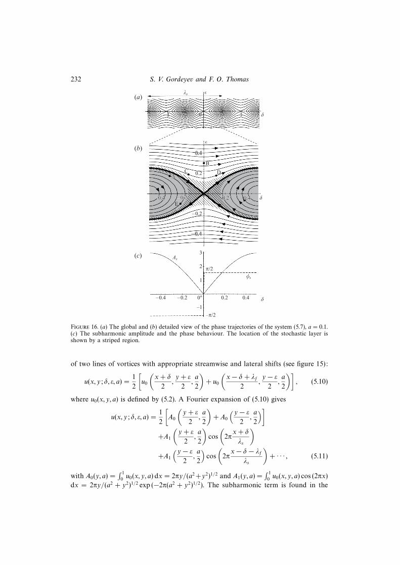
Now the discrete system (5.4) is replaced by the continuous system (5.7) with H∞ inthe form of (5.9), which is much more amenable to theoretical analysis. Moreover,due to the symmetry of (5.7), the numerical instability of (5.4) is removed from thesystem and the physical behaviour of this configuration of vortices can be unambiguouslyinvestigated. For Hamiltonian systems, H∞ is the invariant of the system (the energyinvariant), e.g. H∞(δ, ε) = const. along trajectories (δ(t), ε(t)). In other words, theisolines of H∞ show the system behaviour in phase space and this is depicted in figure16(a) and in greater detail in figure 16(b).
The system has three physically distinct fixed points: two centre points at (± 12, 0)
and one saddle point at (0, 0). The saddle point corresponds to the instability of thevortex line, while the two centres show the existence of two regimes where the systemof vortices form interacting pairs. The resulting locations of vortex pairs in bothregimes are shifted with respect to each other a distance of λs/2 = 1.
The velocity field can be found by noticing that the vortex system is a superposition
232 S. V. Gordeyev and F. O. Thomas
εks
–1–1–1 d111000
(a)
(b)ε
0.40.40.4
0.2
–0.2
–0.4–0.4–0.4
–0.4–0.4–0.4 –0.2–0.2–0.2 0.20.20.2 0.40.40.4 dE
AAAC
B
D
(c)
d0.40.2–0.2–0.4
–1
1
2
3As
φs
p/2
–p/2
0°
Figure 16. (a) The global and (b) detailed view of the phase trajectories of the system (5.7), a = 0.1.(c) The subharmonic amplitude and the phase behaviour. The location of the stochastic layer isshown by a striped region.
of two lines of vortices with appropriate streamwise and lateral shifts (see figure 15):
u(x, y; δ, ε, a) =1
2
[u0
(x+ δ
2,y + ε
2,a
2
)+ u0
(x− δ + λf
2,y − ε
2,a
2
)], (5.10)
where u0(x, y, a) is defined by (5.2). A Fourier expansion of (5.10) gives
u(x, y; δ, ε, a) =1
2
[A0
(y + ε
2,a
2
)+ A0
(y − ε2
,a
2
)]+A1
(y + ε
2,a
2
)cos
(2πx+ δ
λs
)+A1
(y − ε2
,a
2
)cos
(2πx− δ − λf
λs
)+ · · · , (5.11)
with A0(y, a) =∫ 1
0u0(x, y, a) dx = 2πy/(a2 +y2)1/2 and A1(y, a) =
∫ 1
0u0(x, y, a) cos (2πx)
dx = 2πy/(a2 + y2)1/2 exp (−2π(a2 + y2)1/2). The subharmonic term is found in the

Temporal subharmonic amplitude and phase behaviour in a jet shear layer 233
form As(δ, ε, a) exp (i(2πx/λs + φs(δ))) with
As(δ, ε, a) = A(ε, a)| sin (2πδ/λs)|,φs(δ) = π/2 sign (sin (2πδ/λs)),
}(5.12)
whose behaviour versus δ for fixed ε is plotted in figure 16(c).The subharmonic mode has two stable points: φ1 = π/2 if sin (πδ) > 0 and
φ2 = −π/2 if sin (πδ) < 0. For a phase-space location in the shaded region (e.g. pointA of figure 16b) framed by a separatrix (shown as a thick dark line) the subharmonicphase φs remains constant and in this sense the region can be called a stable one.In the outer region, when the trajectory (δ(t), ε(t)) crosses the line δ = 0 (point B offigure 16b, for example), the subharmonic phase φs experiences a π-jump while theamplitude As drops to zero as shown in figure 16(c). The similarity between the modelsubharmonic behaviour shown in this figure and the experimental results highlighted inthe inset region of figure 2 is readily apparent.
It is important to know that although the system is deterministic, it is very sensitiveto the conditions in the neighbourhood of the separatrix. Any small variations of εand/or δ can make the system leave a stable region, giving rise to changes in φs, sincetrajectories in the outer region result in π phase jumps and subharmonic amplitudeminima. Alternatively the system could return back to a stable region, where φsremains constant.
Note that the temporal behaviour of the system in the outer region can be de-scribed as a tearing and re-pairing process. The tearing phenomenon implies that theinteraction within a pair of vortices becomes weak, the nascent vortex pair tears apartand the vortices start to behave as isolated ones. In contrast, the temporal behaviourin the inner region corresponds to vortex pairing.
5.2. On the application of the model to the jet shear layer
In the jet shear layer excited at low-amplitude an array of well-defined vortices existsfor 70 < x/θ0 < 200. The fundamental wavelength λf = Uc/ff ≈ 4 mm gives a roughestimate of the distance between vortices which, in turn, suggests that M ≈ 4 − 5spanwise two-dimensional vortices exist in this region at any given time. The theorywhich has been developed is based on an infinite number of vortices and cannotbe applied directly to a finite line of vortices. However, let us consider any pair ofvortices in this line with the corresponding ε and δ. The governing system for thedynamics of the pair is
dε
dt=∂H
∂δ,
dδ
dt= −∂H
∂ε. (5.13)
The Hamiltonian H for the pair of vortices can be written as H = H∞ + ∆H , wherethe Hamiltonian H∞ corresponds to an infinite line of vortices, properly alignedaccording to (5.6) for a given ε and δ, and ∆H is the deviation of the Hamiltoniandue to the difference between this ideal alignment of an infinite number of vorticesand the real finite line of vortices. This difference consists of three parts: (i) theabsence of vortices beyond the finite line of vortices, (ii) misalignment of vorticesfrom a perfectly aligned case (as given by (5.6)) within the finite line and finally (iii)additional disturbances such as the influence from the vortical structures in the otherjet shear layer. One can estimate that the absence of vortices outside of the finiteline contributes ∼ 1/M to ∆H , where M is the number of vortices in the finite line.From the fact that the subharmonic mode is well-defined and there are no other
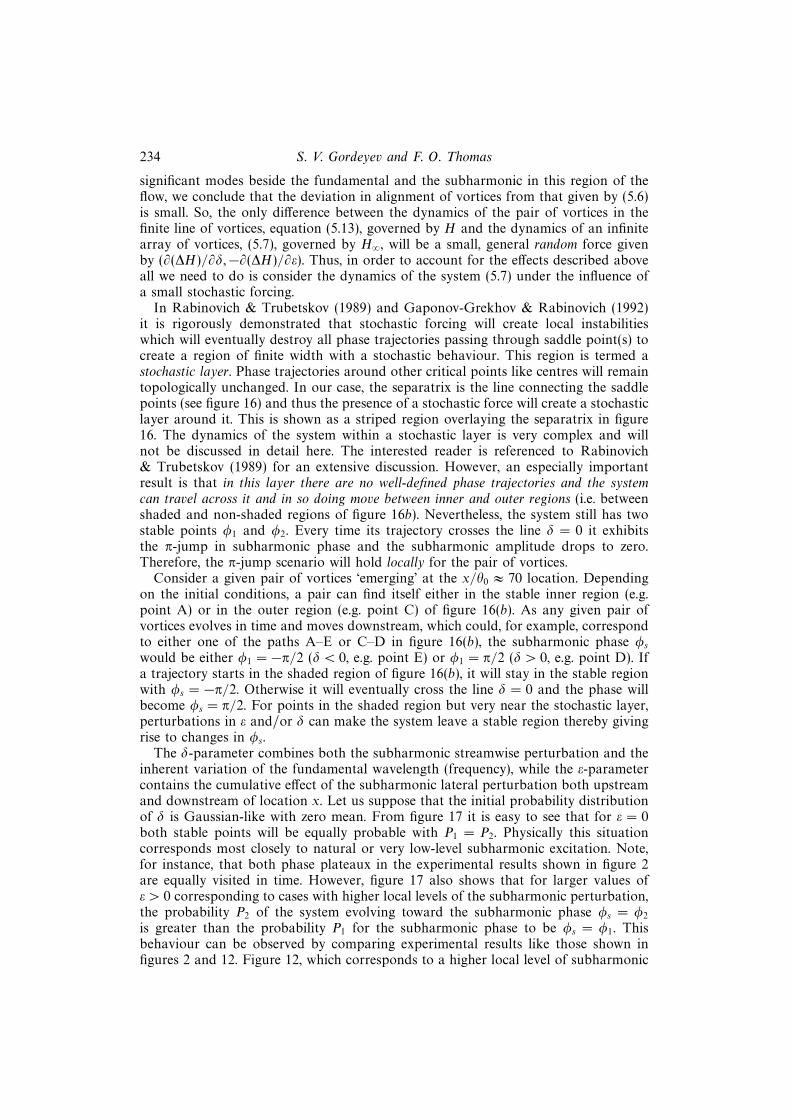
234 S. V. Gordeyev and F. O. Thomas
significant modes beside the fundamental and the subharmonic in this region of theflow, we conclude that the deviation in alignment of vortices from that given by (5.6)is small. So, the only difference between the dynamics of the pair of vortices in thefinite line of vortices, equation (5.13), governed by H and the dynamics of an infinitearray of vortices, (5.7), governed by H∞, will be a small, general random force givenby (∂(∆H)/∂δ,−∂(∆H)/∂ε). Thus, in order to account for the effects described aboveall we need to do is consider the dynamics of the system (5.7) under the influence ofa small stochastic forcing.
In Rabinovich & Trubetskov (1989) and Gaponov-Grekhov & Rabinovich (1992)it is rigorously demonstrated that stochastic forcing will create local instabilitieswhich will eventually destroy all phase trajectories passing through saddle point(s) tocreate a region of finite width with a stochastic behaviour. This region is termed astochastic layer. Phase trajectories around other critical points like centres will remaintopologically unchanged. In our case, the separatrix is the line connecting the saddlepoints (see figure 16) and thus the presence of a stochastic force will create a stochasticlayer around it. This is shown as a striped region overlaying the separatrix in figure16. The dynamics of the system within a stochastic layer is very complex and willnot be discussed in detail here. The interested reader is referenced to Rabinovich& Trubetskov (1989) for an extensive discussion. However, an especially importantresult is that in this layer there are no well-defined phase trajectories and the systemcan travel across it and in so doing move between inner and outer regions (i.e. betweenshaded and non-shaded regions of figure 16b). Nevertheless, the system still has twostable points φ1 and φ2. Every time its trajectory crosses the line δ = 0 it exhibitsthe π-jump in subharmonic phase and the subharmonic amplitude drops to zero.Therefore, the π-jump scenario will hold locally for the pair of vortices.
Consider a given pair of vortices ‘emerging’ at the x/θ0 ≈ 70 location. Dependingon the initial conditions, a pair can find itself either in the stable inner region (e.g.point A) or in the outer region (e.g. point C) of figure 16(b). As any given pair ofvortices evolves in time and moves downstream, which could, for example, correspondto either one of the paths A–E or C–D in figure 16(b), the subharmonic phase φswould be either φ1 = −π/2 (δ < 0, e.g. point E) or φ1 = π/2 (δ > 0, e.g. point D). Ifa trajectory starts in the shaded region of figure 16(b), it will stay in the stable regionwith φs = −π/2. Otherwise it will eventually cross the line δ = 0 and the phase willbecome φs = π/2. For points in the shaded region but very near the stochastic layer,perturbations in ε and/or δ can make the system leave a stable region thereby givingrise to changes in φs.
The δ-parameter combines both the subharmonic streamwise perturbation and theinherent variation of the fundamental wavelength (frequency), while the ε-parametercontains the cumulative effect of the subharmonic lateral perturbation both upstreamand downstream of location x. Let us suppose that the initial probability distributionof δ is Gaussian-like with zero mean. From figure 17 it is easy to see that for ε = 0both stable points will be equally probable with P1 = P2. Physically this situationcorresponds most closely to natural or very low-level subharmonic excitation. Note,for instance, that both phase plateaux in the experimental results shown in figure 2are equally visited in time. However, figure 17 also shows that for larger values ofε > 0 corresponding to cases with higher local levels of the subharmonic perturbation,the probability P2 of the system evolving toward the subharmonic phase φs = φ2
is greater than the probability P1 for the subharmonic phase to be φs = φ1. Thisbehaviour can be observed by comparing experimental results like those shown infigures 2 and 12. Figure 12, which corresponds to a higher local level of subharmonic
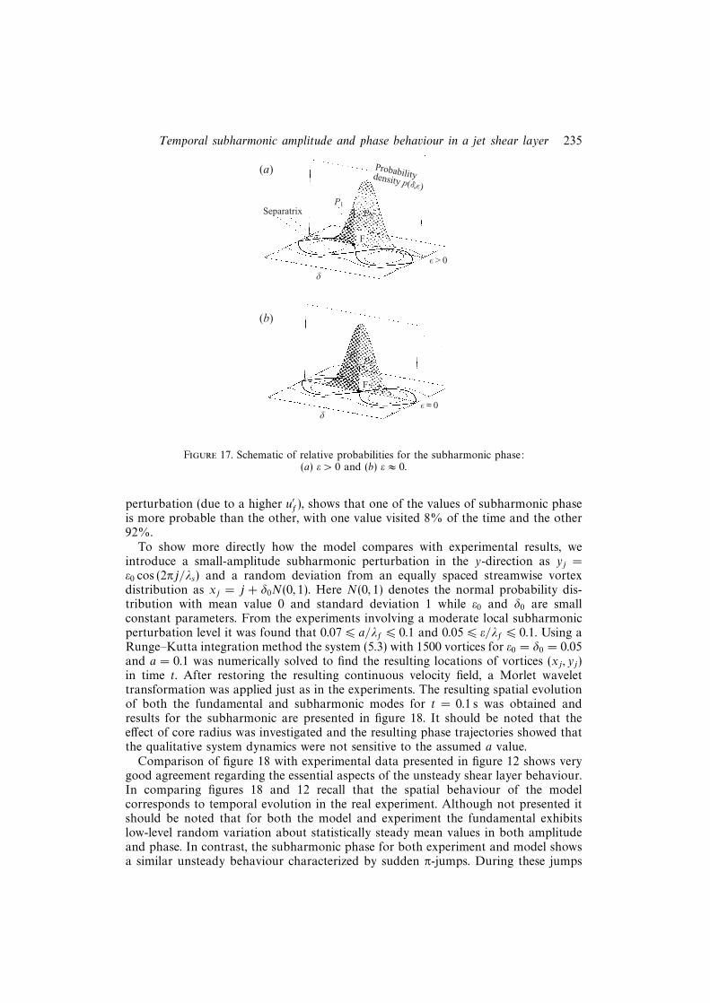
Temporal subharmonic amplitude and phase behaviour in a jet shear layer 235
d
(a)
(b)
Separatrix
Probabilitydensity p(δ,ε)
F
P1
P2
ε > 0
d
F
P1 P2
ε ≈ 0
Figure 17. Schematic of relative probabilities for the subharmonic phase:(a) ε > 0 and (b) ε ≈ 0.
perturbation (due to a higher u′f), shows that one of the values of subharmonic phaseis more probable than the other, with one value visited 8% of the time and the other92%.
To show more directly how the model compares with experimental results, weintroduce a small-amplitude subharmonic perturbation in the y-direction as yj =ε0 cos (2πj/λs) and a random deviation from an equally spaced streamwise vortexdistribution as xj = j + δ0N(0, 1). Here N(0, 1) denotes the normal probability dis-tribution with mean value 0 and standard deviation 1 while ε0 and δ0 are smallconstant parameters. From the experiments involving a moderate local subharmonicperturbation level it was found that 0.07 6 a/λf 6 0.1 and 0.05 6 ε/λf 6 0.1. Using aRunge–Kutta integration method the system (5.3) with 1500 vortices for ε0 = δ0 = 0.05and a = 0.1 was numerically solved to find the resulting locations of vortices (xj, yj)in time t. After restoring the resulting continuous velocity field, a Morlet wavelettransformation was applied just as in the experiments. The resulting spatial evolutionof both the fundamental and subharmonic modes for t = 0.1 s was obtained andresults for the subharmonic are presented in figure 18. It should be noted that theeffect of core radius was investigated and the resulting phase trajectories showed thatthe qualitative system dynamics were not sensitive to the assumed a value.
Comparison of figure 18 with experimental data presented in figure 12 shows verygood agreement regarding the essential aspects of the unsteady shear layer behaviour.In comparing figures 18 and 12 recall that the spatial behaviour of the modelcorresponds to temporal evolution in the real experiment. Although not presented itshould be noted that for both the model and experiment the fundamental exhibitslow-level random variation about statistically steady mean values in both amplitudeand phase. In contrast, the subharmonic phase for both experiment and model showsa similar unsteady behaviour characterized by sudden π-jumps. During these jumps

236 S. V. Gordeyev and F. O. Thomas
3
2
1
0–100 –50 0 50 100
Sub
. am
p.(a
rb. u
nits
)
p
p/2
0
–p/2
–p–100 –50 0 50 100
φs (
rad)
x
Figure 18. Computed spatial behaviour of the subharmonic mode after 0.1 s. ε0 = δ0 = 0.05.
3
2
1
0–100 –50 0 50 100
Sub
. am
p.(a
rb. u
nits
)
p
p/2
0
–p/2
–p–100 –50 0 50 100
φs (
rad)
x
Figure 19. Computed spatial behaviour of the the subharmonic mode after 0.1 s.ε0 = 0.0001, δ0 = 0.05.
the subharmonic amplitude approaches zero in both experiment and model. Theexperiment shows a much greater probability for one value of subharmonic phasethan the other possible value and this is also in agreement with the model result.
Consider next the case of very small local subharmonic perturbation correspondingto ε ≈ 0. Computational results are presented in figure 19 for ε0 = 0.0001, δ0 = 0.05,t = 0.1 s. Now the system is observed to visit both subharmonic phase values equallyin time which is consistent with the experimental results presented in figure 2.
The computational results shown in figures 18 and 19 are consistent with thediscussion surrounding figure 17 and demonstrate how the subharmonic phase canspend more time at one phase value than another for moderate local subharmonicexcitation.
It is important to note the difference between temporal π-jumps in phase forthe natural subharmonic mode and the π-shifts in average effective F–S phase angle

Temporal subharmonic amplitude and phase behaviour in a jet shear layer 237
between pairing and tearing regimes as observed in the bimodal forcing experiments(figures 6 and 7). Sustained vortex tearing is not observed in experiments involvingthe naturally occurring subharmonic. Even in the experiments involving bimodalexcitation, in which local subharmonic suppression is achieved by proper selection ofφin, it was found that such regions are characterized by a high level of temporal phasevariation. This is because the vortex tearing regime is associated with an unstablesaddle point in phase space. Consequently trajectories will not remain there for thenatural subharmonic and even with artificial excitation of the subharmonic it isdifficult to keep the phase trajectory near the saddle point. In fact, application of thewavelet transform to regions of the flow characterized by subharmonic suppression inthe bimodal forcing experiments showed temporal subharmonic amplitude and phasebehaviour which is similar in character to that observed in experiments involving thenatural subharmonic. In contrast, regions of strong subharmonic growth are foundto be associated with little temporal phase variation, a consequence of the stabilityinherent in the two fixed points. In the bimodal forcing experiments, the streamwisevariation in the local effective F–S phase for φin corresponding to vortex pairing andtearing are separated by π radians for x-stations where the subharmonic is suppressed.This is consistent with the Hamiltonian model. When the system is forced to be in anunstable tearing regime the trajectory lies in the neighbourhood of the saddle pointin figure 16(b). This corresponds to the case of φs = 0 and As ≈ 0 (see figure 16c),while the pairing scenario corresponds to φs =± π/2 and peak amplitude As (i.e. thecentres in figure 16a). The difference in local effective F–S phase angle between casesis [φeff ] = [φf]− 2[φs], where [·] denotes the difference in values between the pairingand tearing regimes. As [φf] = 0, [φeff ] = −2[φs] = −2(± π/2) = ∓ π as indicated inthe experimental results shown in figures 5, 6 and 7.
The model reflects all essential features of the vortex interactions within the shearlayer: the unsteady subharmonic amplitude variation and the existence of two pseudo-stable phase points with sudden π-jumps between them. The phase excursions and theamplitude drops occur at the same time.
The dissipative effect of viscosity will change centre points into stable foci whichis equivalent to the eventual merging of two pairing vortices into one. However, itis important to note that viscosity will leave the saddle point unchanged so that theπ-jump scenario will still hold in the presence of viscosity.
Of course, since the model is inherently two-dimensional it will fail to apply atstreamwise locations well downstream of vortex pairing where the initially span-wise coherent vortex filaments become three-dimensional and mixing transition hasoccurred.
6. SummaryIn experiments utilizing excitation of only the fundamental mode over the range
0.002% 6 u′f 6 0.1%, the naturally developing subharmonic exhibits an interestingtemporal amplitude and phase variation that has not been previously reported. Thistakes the form of intermittent π-shifts in subharmonic phase between two fixed phasevalues. These phase jumps are observed to be highly correlated with the local dropsto a near zero value of the subharmonic amplitude. In contrast, the fundamentalamplitude and phase show no such behaviour, exhibiting only low levels of temporalmodulation. The temporal phase behaviour of the subharmonic has the effect ofintermittently disrupting the phase lock with the fundamental. Similar behaviour is
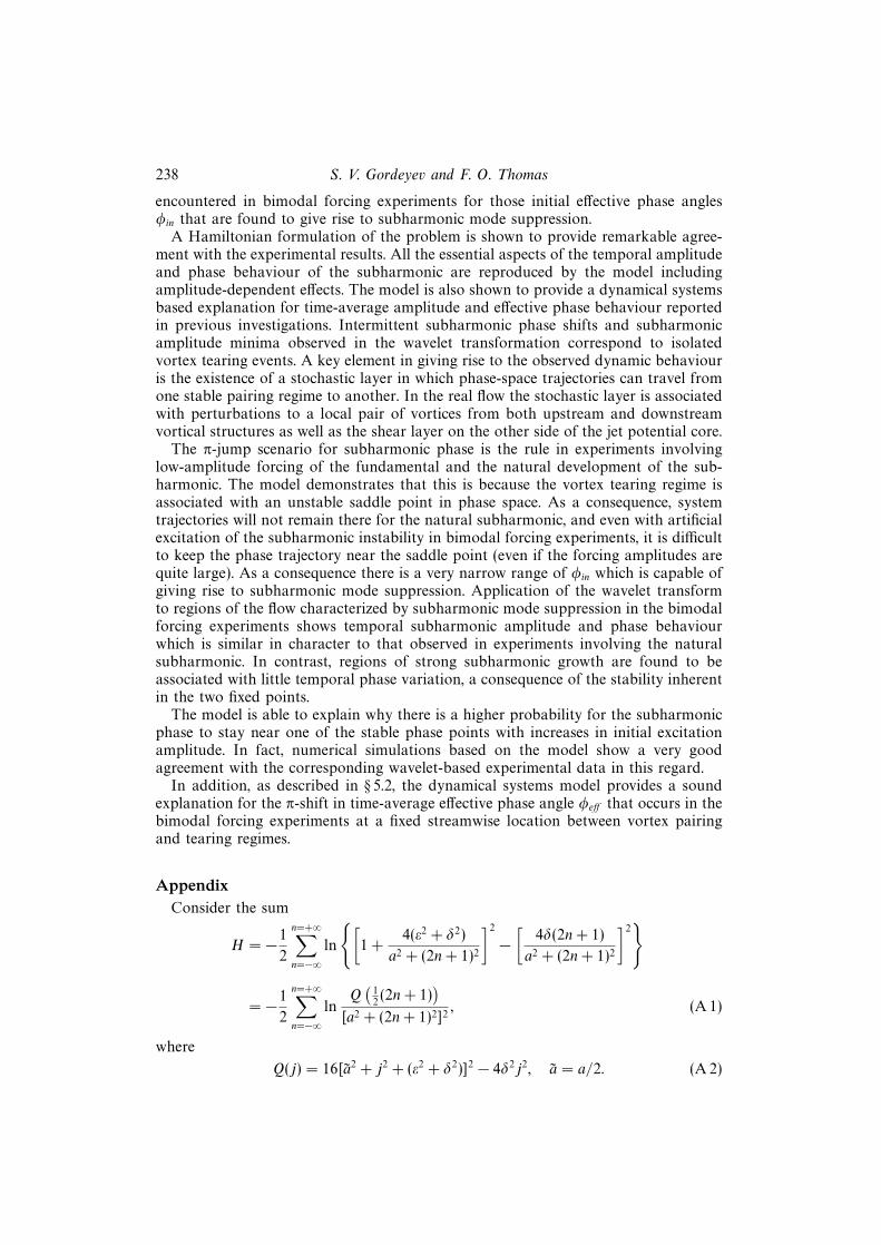
238 S. V. Gordeyev and F. O. Thomas
encountered in bimodal forcing experiments for those initial effective phase anglesφin that are found to give rise to subharmonic mode suppression.
A Hamiltonian formulation of the problem is shown to provide remarkable agree-ment with the experimental results. All the essential aspects of the temporal amplitudeand phase behaviour of the subharmonic are reproduced by the model includingamplitude-dependent effects. The model is also shown to provide a dynamical systemsbased explanation for time-average amplitude and effective phase behaviour reportedin previous investigations. Intermittent subharmonic phase shifts and subharmonicamplitude minima observed in the wavelet transformation correspond to isolatedvortex tearing events. A key element in giving rise to the observed dynamic behaviouris the existence of a stochastic layer in which phase-space trajectories can travel fromone stable pairing regime to another. In the real flow the stochastic layer is associatedwith perturbations to a local pair of vortices from both upstream and downstreamvortical structures as well as the shear layer on the other side of the jet potential core.
The π-jump scenario for subharmonic phase is the rule in experiments involvinglow-amplitude forcing of the fundamental and the natural development of the sub-harmonic. The model demonstrates that this is because the vortex tearing regime isassociated with an unstable saddle point in phase space. As a consequence, systemtrajectories will not remain there for the natural subharmonic, and even with artificialexcitation of the subharmonic instability in bimodal forcing experiments, it is difficultto keep the phase trajectory near the saddle point (even if the forcing amplitudes arequite large). As a consequence there is a very narrow range of φin which is capable ofgiving rise to subharmonic mode suppression. Application of the wavelet transformto regions of the flow characterized by subharmonic mode suppression in the bimodalforcing experiments shows temporal subharmonic amplitude and phase behaviourwhich is similar in character to that observed in experiments involving the naturalsubharmonic. In contrast, regions of strong subharmonic growth are found to beassociated with little temporal phase variation, a consequence of the stability inherentin the two fixed points.
The model is able to explain why there is a higher probability for the subharmonicphase to stay near one of the stable phase points with increases in initial excitationamplitude. In fact, numerical simulations based on the model show a very goodagreement with the corresponding wavelet-based experimental data in this regard.
In addition, as described in § 5.2, the dynamical systems model provides a soundexplanation for the π-shift in time-average effective phase angle φeff that occurs in thebimodal forcing experiments at a fixed streamwise location between vortex pairingand tearing regimes.
AppendixConsider the sum
H = −1
2
n=+∞∑n=−∞
ln
{[1 +
4(ε2 + δ2)
a2 + (2n+ 1)2
]2
−[
4δ(2n+ 1)
a2 + (2n+ 1)2
]2}
= −1
2
n=+∞∑n=−∞
lnQ(
12(2n+ 1)
)[a2 + (2n+ 1)2]2
, (A 1)
where
Q(j) = 16[a2 + j2 + (ε2 + δ2)]2 − 4δ2j2, a = a/2. (A 2)
Temporal subharmonic amplitude and phase behaviour in a jet shear layer 239
Consider
∂H
∂ε= −1
2
n=+∞∑n=−∞
∂Q(
12(2n+ 1)
)∂ε
Q(
12(2n+ 1)
) = −1
2
n=+∞∑n=−∞
f
((2n+ 1)
2
). (A 3)
Use the Mittag–Leffler’s formula,
n=+∞∑n=−∞
f(
12(2n+ 1)
)= π
∑all poles of f(z)
Res{tan πz f(z)}. (A 4)
Poles of f(z) correspond to zeros of the polynomial Q(z). Q(z) has four zeros:z1,2,3,4 = ± δ ± i
√a2 + ε2. For the z’s
tan πz1,2,3,4 =1
2
± sin (2πδ) ± i sinh√a2 + ε2
cos2 πδ + sinh2 (π√a2 + ε2)
, (A 5)
Res f(z1,3) = −Res f(z2,4) = −iε√
a2 + ε2. (A 6)
Finally
∂H
∂ε= − πε√
a2 + ε2
sinh (2π√a2 + ε2)
cos2 (πδ) + sinh2 (π√a2 + ε2)
. (A 7)
Similarly,
∂H
∂δ= −1
2
n=+∞∑n=−∞
∂Q(
12(2n+ 1)
)∂δ
Q(
12(2n+ 1)
) = −1
2
n=+∞∑n=−∞
g
((2n+ 1)
2
)(A 8)
with the final result
∂H
∂δ= π
sin (2πδ)
cos2 (πδ) + sinh2 (π√a2 + ε2)
. (A 9)
Reconstruction of H from ∂H/∂ε and ∂H/∂δ gives
H(δ, ε) = − 12
log[cos2 (πδ) + sinh2 (π
√(a/2)2 + ε2)
]. (A 10)
REFERENCES
Arbey, H. & Ffowcs Williams, J. E. 1984 Active cancellation of pure tones in an excited jet.J. Fluid Mech. 149, 445–454.
Batchelor, G. K. 1967 An Introduction to Fluid Dynamics. Cambridge University Press.
Bendat, J. S. & Piersol, A. G. 1986 Random Data: Analysis and Measurement Procedures, 2nd Edn.John Wiley.
Betyayev, S. K., Gaifullin, A. M. & Gordeyev, S. V. 1994 The point-circle vortex. J. Appl. MathsMech. 58(4), 749–754.
Corke, T. C., Shakib, F. & Nagib, H. 1991 Mode selection and resonant phase locking in unstableaxisymmetric jets. J. Fluid Mech. 223, 253–311.
Daubechies, I. 1992 Ten Lectures on Wavelets. Society for Industrial and Applied Mathematics.
Drazin, P. G. & Reid, W. H. 1983 Hydrodynamic Stability. Cambridge University Press.
Farge, M. 1992 Wavelet transforms and their applications to turbulence. Ann. Rev. Fluid Mech. 24,395–457.
240 S. V. Gordeyev and F. O. Thomas
Farge, M., Kevlahan, N., Perrier, V. & Goirand, E. 1996 Wavelets and turbulence. Proc. IEEE84(4), 639–669.
Gaponov-Grekhov, A. V. & Rabinovich, M. I. 1992 Nonlinearities in Action: Oscillations, Chaos,Order, Fractals. Springer.
Hajj, M. R., Miksad, R. W. & Powers, E. J. 1992 Subharmonic growth by parametric resonance.J. Fluid Mech. 236, 385–413.
Hajj, M. R., Miksad, R. W. & Powers, E. J. 1993 Fundamental-subharmonic interaction: effect ofphase relation. J. Fluid Mech. 256, 403–426.
Ho, C. M. & Huang, L. S. 1982 Subharmonics and vortex merging in mixing layers. J. Fluid Mech.119, 443–473.
Huang, L. S. & Ho, C. M. 1990 Small-scale transition in a plane mixing layer. J. Fluid Mech. 210,475–500.
Husain, H. & Hussain, F. 1995 Experiments on subharmonic resonance in a shear layer. J. FluidMech. 304, 343–372.
Kaiser, G. 1994 A Friendly Guide to Wavelets. Birkhauser.
Kelly, R. E. 1967 On the stability of an inviscid shear layer which is periodic in space and time.J. Fluid Mech. 31, 789–99.
Kim, Y. C., Khadra, L. & Powers, E. J. 1980 Wave modulation in a nonlinear dispersive medium.Phys. Fluids, 23, 2250–2257.
Lamb, H. 1945 Hydrodynamics. Dover.
Lewalle, J. 1994 Wavelet analysis of experimental data: some methods and the underlying physics.AIAA Paper 94-2281.
Mankbadi, R. R. 1985 On the interaction between fundamental and subharmonic instability wavesin a turbulent round jet. J. Fluid Mech. 160, 385–419.
Mankbadi, R. R. 1986 The effect of phase difference on the spreading rate of a jet. AIAA J. 24,1941–1948.
Mankbadi, R. R. 1994 Transition, Turbulence, and Noise: Theory and Applications for Scientists andEngineers. Kluwer.
Monkewitz, P. A. 1988 Subharmonic resonance, pairing and shredding in the mixing layer. J. FluidMech. 188, 223–252.
Moore, D. W. & Saffman, P. G. 1975 The density of organized vortices in a turbulent mixing layer.J. Fluid Mech. 69, 465–473.
Rabinovich, M. I. & Trubetskov, D. I. 1989 Oscillations and Waves in Linear and Nonlinear Systems.Kluwer.
Rajaee, M. & Karlsson, S. K. F. 1992 On the Fourier space decomposition of free shear flowmeasurements and mode degeneration in the pairing process. Phys. Fluids A 4, 321–339.
Thomas, F. O. & Chu, H. C. 1991 Experimental investigation of the nonlinear spectral dynamicsof planar jet transition. Phys. Fluids 3, 1544–1559.
Thomas, F. O. & Chu, H. C. 1993a Nonlinear wave coupling and subharmonic resonance in planarjet shear layer transition. Phys. Fluids A 5, 630–646.
Thomas, F. O. & Chu, H. C. 1993b Experiments on the nonlinear stages of excited jet shear layertransition. Exps. Fluids 14, 451–467.
Yang, Z. & Karlsson, S. K. F. 1991 Evolution of coherent structures in a plane shear layer. Phys.Fluids A 3, 2207–2219.
Zhang, Y. Q., Ho, C. M. & Monkewitz, P. 1983 The mixing layer forced by fundamental andsubharmonic in laminar-turbulent transition. IUTAM Symp, Novosibirsk, USSR (ed. V. V.Kozlov), pp. 385–395. Springer.