temporal interpolation methods for the clouds and the

572 VOLUME 37J O U R N A L O F A P P L I E D M E T E O R O L O G Y

q 1998 American Meteorological Society

Temporal Interpolation Methods for the Clouds and the Earth’s RadiantEnergy System (CERES) Experiment

D. F. YOUNG AND P. MINNIS

Atmospheric Sciences Division, NASA/Langley Research Center, Hampton, Virginia

D. R. DOELLING

Analytical Services & Materials, Inc., Hampton, Virginia

G. G. GIBSON AND T. WONG

Atmospheric Sciences Division, NASA/Langley Research Center, Hampton, Virginia

(Manuscript received 31 May 1997, in final form 31 October 1997)

ABSTRACT

The Clouds and the Earth’s Radiant Energy System (CERES) is a NASA multisatellite measurement programfor monitoring the radiation environment of the earth–atmosphere system. The CERES instrument was flownon the Tropical Rainfall Measuring Mission satellite in late 1997, and will be flown on the Earth ObservingSystem morning satellite in 1998 and afternoon satellite in 2000. To minimize temporal sampling errors associatedwith satellite measurements, two methods have been developed for temporally interpolating the CERES earthradiation budget measurements to compute averages of top-of-the-atmosphere shortwave and longwave flux.The first method is based on techniques developed from the Earth Radiation Budget Experiment (ERBE) andprovides radiation data that are consistent with the ERBE processing. The second method is a newly developedtechnique for use in the CERES data processing. This technique incorporates high temporal resolution data fromgeostationary satellites to improve modeling of diurnal variations of radiation due to changing cloud conditionsduring the day. The performance of these two temporal interpolation methods is evaluated using a simulateddataset. Simulation studies show that the introduction of geostationary data into the temporal interpolation processsignificantly improves the accuracy of hourly and daily radiative products. Interpolation errors for instantaneousflux estimates are reduced by up to 68% for longwave flux and 80% for shortwave flux.

1. Introduction

Global radiation budget measurements at the top ofthe atmosphere (TOA) are fundamental quantities formonitoring the earth’s climate system. These importantclimatic measurements have traditionally been obtainedfrom earth radiation budget (ERB) instruments on boardpolar-orbiting satellites. While these satellites are ca-pable of viewing the entire earth’s surface from theNorth Pole to the South Pole over a number of satelliteorbital passes, they do not, however, provide continuousspatial coverage of the earth’s entire surface at any onespecific time or continuous temporal coverage for anyone specific location on the earth. The sparse distri-bution of these satellite measurements is the most crit-ical factor affecting temporal averaging of radiation datafrom regional to global scales (Brooks et al. 1986). To

Corresponding author address: Mr. David F. Young, NASA/LangleyResearch Center, Mail Stop 420, Hampton, VA 23681.E-mail: [email protected]

overcome these sampling problems and to recapture theproper daily or monthly average of these radiation pa-rameters, realistic temporal models of the diurnal vari-ability of the earth’s radiation fields are required. Spe-cifically, these diurnal models must adequately accountfor the solar zenith dependence of albedo and longwaveexitance, as well as dependence of the radiation fieldon surface type and cloud cover.

Early radiation budget satellite experiments in themid-1970s used very simple procedures to obtain dailyaverages of longwave (LW) and reflected shortwave(SW) radiation. For example, National Oceanic and At-mospheric Administration (NOAA) scanning radiome-ter data (Gruber and Winston 1978) and Nimbus-6 ERBexperiment (Jacobowitz et al. 1979) data assumed thatdaily albedo in a region equals the albedo at the localtime of the measurement and ignored the substantialdiurnal variation of albedo with solar zenith angle andchanges of cloudiness during the day. Similarly, dailyLW flux was computed as the unweighted mean of day-time and nighttime measurements and neglected the im-portance of the diurnal cycle of LW flux, which is es-

JUNE 1998 573Y O U N G E T A L .

FIG. 1. Temporal coverage of CERES satellites.

pecially pronounced over land and desert regions. Thesetemporal modeling problems were reduced by incor-porating empirical surface-dependent albedo models de-veloped from Nimbus-2 and -3 satellite data to accountfor solar-zenith-angle dependence of reflected SW fluxand length-of-day weighting factors in averaging thedaytime and nighttime LW flux (Raschke et al. 1973;Raschke and Bandeen 1970). Further developments andimprovements of the surface-dependent angular reflec-tance models continued in the early 1980s using Nim-bus-7 radiance data (Taylor and Stowe 1984). Theseimproved models were applied to the Nimbus-7 mea-surements to obtain radiation budget data with correc-tions to daily albedo based on models from Nimbus-3.

The launch of the Earth Radiation Budget Experiment(ERBE; Barkstrom 1984; Barkstrom and Smith 1986)in the mid-1980s opened a new chapter in earth radiationbudget measurements. ERBE incorporated many tech-nological advances in instrumentation, as well as im-proved techniques for diurnal averaging. For example,12 new directional models based on Nimbus-7 and Ge-ostationary Operational Environmental Satellite(GOES) measurements (Suttles et al. 1988) were usedto refine diurnal interpolation of albedo. A new half-sine model based on GOES observations (Brooks andMinnis 1984a) was used to improve the diurnal inter-polation of LW flux over desert and vegetated land sur-faces. In addition, ERBE made the first attempt to ac-count for diurnal variations in clouds by measuring theradiation budget with multiple satellites (Harrison et al.1983). This multisatellite system included the precess-ing Earth Radiation Budget Satellite (ERBS), whichsampled latitudes between 608S and 608N and coveredall local times at the equator in 36 days, and the NOAA-9 and -10 sun-synchronous satellites with nominal as-cending node equatorial crossing times of 1430 and1930 local standard time (LST), respectively. This com-bination of multiple satellites and new diurnal modelshas produced the most accurate monthly mean regionalalbedos and LW fluxes to date (Harrison et al. 1988;Harrison et al. 1990; Barkstrom et al. 1990), as well asthe best estimates of the diurnal variability of TOA ra-diative fluxes (Harrison et al. 1988; Hartmann et al.1991).

The ERBS and NOAA-9 scanning radiometers oper-ated together for 2 years from February 1985 throughJanuary 1987, while ERBS and NOAA-10 scanned si-multaneously from December 1986 through May 1989.The highest accuracy was achieved during the 1 monthwhen all three satellites had operating scanners. Thetwo-satellite combinations represent a significant im-provement over a single satellite (e.g., Brooks and Min-nis 1984b). In some regions, however, errors in themonthly mean diurnal cycle of LW and SW fluxes canstill be significant due to deviations from the assumedmodels.

The Clouds and the Earth’s Radiant Energy System(CERES; Wielicki et al. 1996) is planned for flight on

multiple satellite platforms starting in 1997 with theTropical Rainfall Measuring Mission (TRMM) and onthe Earth Observing System Morning Satellite and Af-ternoon Satellite (EOS-AM and EOS-PM) missions in1998 and 2000, respectively. CERES represents a con-tinuation of the ERBE dataset as well as an evolutionin ERB technology to obtain more accurate satellitemeasurements and to develop and apply improved di-urnal models. The temporal coverage of the three CE-RES satellites (TRMM, EOS-AM, and EOS-PM) for 1month of observations is shown in Fig. 1. The TRMMspacecraft is in a 358 inclined, precessing orbit that cov-ers all local times at the equator in slightly over 23 days.The EOS satellites are in sun-synchronous orbits, sam-pling at the same local times each day. From Fig. 1, itis evident that a single satellite cannot provide sufficienttemporal sampling to accurately estimate SW and LWfluxes at all local hours. As with ERBE, the applicationof diurnal models will be required to obtain accuratemonthly averages of radiation parameters. Also, thegoals of CERES are more ambitious in that accuratehourly flux estimates are desired in addition to themonthly averages obtained by ERBE.

As ERB satellite instrumentation has steadily im-proved over the years, models and methods for aver-aging and interpreting the data have undergone a similarevolutionary trend. From simple linear averaging to themore physically realistic ERBE models, the science ofdiurnal modeling attempts to expand the limited numberof measurements into a complete time series of ERBinformation. The ERBE data analysis philosophy dic-tated the application of time–space averaging (TSA)methods that do not require any auxiliary data. Whilethis approach proved quite successful in obtainingmonthly average radiative parameters, individual daysand hours were not accurately estimated. For future ERBmissions such as CERES, a new TSA method will beexplored involving the use of auxiliary geostationarysatellite data to account for changing meteorologicalconditions during the day. Geostationary satellites canobtain a very high temporal sampling of their field ofview, but data are typically available only every 3 h ona global basis (e.g., the International Satellite CloudClimatology Project dataset).


FIG. 2. ERBE models with variation of albedo as a function of so-lar zenith angle.

This paper describes and evaluates the new temporalinterpolation methods for CERES, the next generationof ERB satellite missions. CERES will produce monthlymean TOA fluxes using two methods. The first productwill be produced in a manner identical with that usedby ERBE. Since the ERBE TSA technique has evolvedsignificantly since it was first described by Brooks etal. (1986), the first section of this paper documents itsevolution. The subsequent section details a methodologyfor using geostationary data in the diurnal averagingprocess during the CERES mission. The expected im-provement in accuracy of the geostationary-data-en-hanced method relative to the ERBE methodology isalso described.

2. Method I: ERBE-like time–space averaging

The chief input to CERES time–space averaging is astream of satellite observations of SW and LW TOAflux. Included with each pixel measurement are the sat-ellite viewing geometry, the latitude and longitude ofthe observation, the underlying geographic scene type,and the cloud category for the observed area. Additionalinput data include the solar declination angle and di-rectional albedo models based on the angular distribu-tion models (ADMs) of Suttles et al. (1988). The TSAprocess produces means of TOA SW and LW fluxes onvarious timescales ranging from hourly to monthly andon regional, zonal, and global spatial scales. Separateaverages are computed for clear-sky and total-skyfluxes.

The ERBE methodology for temporally interpolatingLW and SW radiation to all hours of the day for bothclear-sky and total-sky conditions is outlined below.

a. Spatial averaging and temporal corrections

The first step in the averaging process is to sort thechronologically ordered stream of flux measurements inspace and time. Spatially, these data are averaged andprocessed on a geographical grid (e.g., 2.58 3 2.58 forERBE). Each region (grid box) is processed indepen-dently from all others. Within each region, a month ofERB measurements is sorted and averaged into localtime intervals of 1 h (referred to as hour boxes). Thereis a maximum of 744 hour boxes in a month (24 h perday times 31 days).

The averaging of the LW flux is straightforward. Allobservations from a region that were measured withinan hour box are linearly combined. Since albedo is afunction of solar zenith angle, each SW measurementis first corrected to the central time, latitude, and lon-gitude of the regional hour box into which it is collected.The temporal correction is performed using the set ofADMs. As shown in Fig. 2, there are separate ADMsfor the different clear-sky geographical scene types(ocean, land, snow, desert, and coast). The four ERBEcloud cover classes are clear (less than 5%), partly

cloudy (5%–50%), mostly cloudy (50%–95%), andovercast (greater than 95%). Over land and ocean sur-faces, there are models for partly cloudy and mostlycloudy ERBE scene classifications. The various cloudmodels over land are also used over desert and snowregions. A single model is used for overcast conditionsover all surfaces. The ADMs for partly and mostlycloudy coastal scenes are not shown. Within each hourbox, a separate mean albedo is calculated for each cloudclass. The geographic scene type for each region is con-stant for a month.

b. Total-sky TOA LW flux

The ERBE TSA algorithm was designed to providedaily model fits to the TOA LW flux data, as well asmonthly averages of these data. To accomplish this goal,an estimate of LW flux is made for every hour box.This interpolation is performed in one of two ways,depending on the geographic scene type of the region.

Over ocean regions, there is little diurnal variabilityin LW flux due to solar insolation. The greatest varia-


FIG. 3. Time series of ERBS and NOAA-9 ERBE scanner TOA LW flux data and diurnalmodels for a 2.58 region in eastern New Mexico in April 1985.

tions in LW flux over the oceans occur due to changesin the amount and types of clouds. Therefore, no attemptis made to develop complex models for estimating theLW flux between the times of observations. Rather, itis assumed that changes in LW flux are due to changesin cloud conditions, and that such changes are linear.Thus, linear interpolation is used to provide a value ofLW flux for each hour box not observed by the satellite.At the beginning of the month, all hours preceding thefirst observation are filled with the value from the firstobserved time. Similarly, the final measurement at theend of the month serves as the value for all remaininghours in the month. This technique is also used forregions designated as either snow-covered or coastal.

Over land and desert regions, the effects of solar heat-ing are much more pronounced than over ocean regions.During relatively cloud-free periods, there is a generallysinusoidal variation in LW flux over the daylight hours(e.g., Minnis and Harrison 1984). To account for thisvariation, the LW flux for land and desert regions isinterpolated in the following manner. For any day inwhich an observation was made during daylight hours,and during the preceding and following nights, the LWflux for the remaining daylight hours is modeled byfitting a half-sine curve to the observations. Linear in-terpolation substitutes for the half-sine modeling ondays lacking the required observations, or when anydaylight observations of LW flux are less than the ad-jacent nighttime values, or when the resultant half-sinecurve has a negative amplitude.

Longwave interpolation is demonstrated in Fig. 3 us-ing a time series of ERBE scanner data from April 1985over a 2.58 region in eastern New Mexico. In this figure,observations are represented by circles and the inter-polated values are displayed as the solid line. The earlypart of the month was relatively clear, and half-sine fitswere performed on days 1, 2, 4, 6, 7, and 8. During

days 10, 11, and 12, no half-sine fit was used since lowvalues of LW were observed in the late afternoon, in-dicating that clouds must have been developing. In suchcases, the half-sine fit is not realistic and linear inter-polation is used.

When all hour boxes for the month have been filledwith a value of LW flux, daily, monthly–hourly, andmonthly means are calculated using two slightly dif-ferent techniques. In the first method (monthly–daily),a daily mean is computed by averaging the 24 hour boxvalues for each day; the monthly mean TOA LW flux,FLW, is then computed by averaging all of the dailymeans as follows:

D 24

F 5 F (d, h)/24 D, (1)O OLW LW1 2@d51 h51

where FLW(d, h) is the TOA LW flux for day d and localhour h, and D is the total number of days in the month.In the second method (monthly–hourly), hour box val-ues are averaged at each local hour for all days havingan observation. The resulting 24 monthly–hourly meansare then averaged to produce a monthly mean,

24 DLW

F 5 F (d, h)/D 24, (2)O OLW LW LW1 2@d51h51

where DLW is the total number of days in the monthwith at least one LW measurement. The two estimatesof monthly mean LW flux will be equal unless therewere days during the month when no observations weremade.

c. Clear-sky TOA LW flux

The above algorithm works well for total-sky LW fluxin regions that are well sampled over most local times.


FIG. 4. Time series of ERBS and NOAA-9 ERBE scanner clear-sky TOA LW flux data anddiurnal models for a 2.58 region in eastern New Mexico in April 1985.

FIG. 5. ERBE time-averaged monthly–hourly clear-sky TOA LWflux results for the region shown in Fig. 4.

However, problems may arise when applying this tech-nique to clear-sky LW flux data. The ERBE cloud clas-sification procedure is quite restrictive when classifyingan observation as clear (Wielicki and Green 1989). Also,there are many regions over the globe where cloudyconditions prevail throughout the month. Consequently,a region may have a very limited number of clear-skyobservations during the month. In addition, satellitesampling patterns may often cause a local time bias inthe occurrence of clear-sky measurements. An exampleof this is shown in Fig. 4 for the same 2.58 ERBE regionover New Mexico discussed above. For this case, withthe exception of the two measurements from days 4 and5, all of the limited number of clear-sky observationsoccurred during daylight hours. The lack of nighttimedata means that the requirements for performing thediurnal half-sine fits are never met. Linear interpolation

between the times of observation results in an unreal-istically high monthly average because only daytimevalues are available. This problem is particularly seriousover land and desert regions where large diurnal vari-ations in clear-sky LW flux are expected. Since clearocean areas have a much smaller LW flux diurnal vari-ation, the day–night sampling bias should not severelyaffect the ocean monthly means. Therefore, in oceanregions, the clear-sky LW flux is averaged in a manneridentical to the total-sky data.

Because of the problems associated with obtainingaccurate averages of clear-sky LW flux over land anddeserts, the original ERBE TSA algorithm was modifiedto calculate only a single diurnal fit to the monthly en-semble of all clear-sky LW flux data. In the clear-skycase, it is reasonable to process all of the measurementstogether since the variance of measurements at the samelocal hour is expected to be small when compared withthe total sky. There are, of course, some exceptions dueto scene variability of the measurement footprints withinthe region, changing atmospheric conditions such as wa-ter vapor content and temperature during the month,cloud contamination of presumably clear-sky scenes,and possible error due to measurements being made athigh viewing zenith angles. The underlying assumptionis that this variability is small relative to the overalldiurnal variation and can be effectively averaged outfor a region having several clear-sky observations overthe course of a month.

The clear-sky LW flux averaging technique is dem-onstrated in Fig. 5. The data shown in Fig. 4 have beensorted and averaged for the entire month in terms oflocal hour. The daytime points (open symbols) are thenmodeled using a least squares half-sine fit weighted bythe number of measurements at each local hour duringthe month. The nighttime data (filled symbols) are sim-ply averaged and the constant value is used for all night-


FIG. 6. Example of time interpolation of albedo for days with only1 h of observation.

time hours. The monthly mean is then calculated byaveraging the fit over 24 h if the fit meets five basiccriteria.

1) There must be at least one daylight measurementlocated more than 1 h from the terminator.

2) There must be at least one nighttime measurement.3) The least squares half-sine fit to the daylight data

produces a positive amplitude.4) The peak value of the fit must not exceed 400 W

m22.5) The length of day 15 of the month must be greater

than 2 h.

If these criteria are not met, no monthly mean TOALW clear-sky flux is calculated for the region. Since themodeling process is performed on data accumulatedthroughout the month, daily means are not calculatedfor land and desert regions.

This technique produces realistic values of monthlymean clear-sky LW flux, even in regions with sparsedata sampling. However, there are many regions whereno estimate can be made due to the total lack of night-time, clear-sky data due to persistent overcast conditionsor the overly restrictive ERBE clear classificationscheme. To compensate for missing nighttime data, theclear-sky averaging algorithm attempts to correct for themisclassification of nighttime clear pixels as partlycloudy. For each nighttime hour box over land regions,a new clear-sky amount is estimated by assuming that10% of the pixels classified as partly cloudy are actuallyclear when the region is classified as at least 50% partlycloudy. This is consistent with the mean ratio of clearto partly cloudy scene identification by ERBE in thedaytime under these conditions. This new clear-skyamount can be used to calculate a value of clear-skyflux using the mean and standard deviation of the ob-served fluxes. If the maximum observed flux exceedsthis value, then it is assumed to be clear and is used inthe clear-sky averaging process. Although the globalincrease in clear-sky amount is slight (approximately2%), the number of regions with no monthly mean clear-sky value is reduced by 60%–70%.

d. Total-sky and clear-sky TOA SW flux

The problem of producing diurnal, monthly–hourly,and monthly means of SW flux presents a different setof challenges from those associated with the LW flux.Because TOA SW flux is only pertinent to daylighthours, the problems involved in interpolating sparselysampled LW data across day–night boundaries are notencountered. Furthermore, as shown in Fig. 2, thereexist well-developed models of the variation of albedowith solar zenith angle for various clear and cloudybackgrounds (Suttles et al. 1988). These ADMs can beused to interpolate observations to other times of theday. The clear-sky SW flux (or albedo) can be modeledin the same manner as the total sky. The difficulties

involved with the lack of nighttime clear-sky data arenot a factor for SW interpolation.

For each hour box with at least one observation, amean albedo is calculated for each of the four ERBEcloud classifications: clear, partly cloudy, mostly cloudy,and overcast. A relative frequency histogram of eachcloud classification is also stored. Because the temporalchanges of SW radiation may be pronounced even with-in a single hour, measured values are first adjusted tothe nearest local solar half-hour using the ADMs. Fora given surface type and cloud cover category (i.e.,scene type for selecting an ADM), the normalized ADMfunction, d, is defined as the ratio of the ADM albedoat time t and the ADM albedo for overhead sun:

dl[m0(t)] 5 ,a [m (t)]/a (m 5 1)mod 0 mod 0i i(3)

where m0 is the cosine of the solar zenith angle andis the ADM albedo for scene type i (from Fig. 2).amodi

The albedo at any time t9 (e.g., at the local solar half-hour) can be expressed as the product of the observedalbedo and the ratio of the normalized ADM functionsfrom t9 and the time of observation, tobs:

ai(t9) 5 ai[m0(tobs)]di[m0(t9)]/di[m0(tobs)]. (4)

For days with only one measurement of SW flux, eachof the four cloud-type albedos from the hour of obser-vation is modeled at all daylight hours using (4). Thismodeling is illustrated in Fig. 6. The albedos for thefour cloud types are then recombined by weighting eachcloud type albedo with the appropriate areal coveragefraction to obtain the mean albedo for each hour for theentire region (solid line in Fig. 6). The relative abun-dance of the cloud classifications is assumed to remainconstant throughout the day.

For days with more than one measurement, this tech-nique is modified as illustrated in Fig. 7. All daylight


FIG. 7. Example of time interpolation of albedo with 2 h of obser-vation during a day.

hours preceding the first measurement of the day andfollowing the last measurement assume a constant cloudclass from the nearest measurement. These hours aremodeled using (4) as in the single measurement case.For hours between two measurements, it is assumed thatthe cloud histograms are varying linearly over that span.The four cloud-type albedos are modeled from eachsurrounding measurement using (4). Total albedo foreach hour between the two measurements is then pro-duced by inversely weighting the two estimates by thetime from the hour of interest.

Monthly means are calculated when all hours arefilled with albedo values for days with at least one mea-surement. Shortwave flux at each hour h of a given dayd is

FSW(d, h) 5 E0(d)m0(d, h)a(d, h), (5)

where E0 is the mean daily distance-corrected solar con-stant. The SW flux is summed over all hours of dayswith measurements and divided by a summation of solarincident flux over the same hours to produce a monthlymean albedo:

D 24SW

a 5 F (d, h)/24 D /S , (6)O O SW SW 01 2@d51 h51

where FSW(d, h) is the TOA SW flux for day d and localhour h, DSW is the total number of days in the monthwith at least one SW measurement, and S0 is the summedsolar incident SW flux. Monthly mean SW flux, FSW,is then calculated by multiplying monthly mean albedoby the incident solar flux integrated and averaged overall hours of the month

FSW 5 a ,S90 (7)

where is the integrated solar incident SW flux.S90Means for the clear-sky SW flux are produced in a

similar manner. In fact, the process is simpler than forthe total-sky flux since only the clear albedo from eachhour box needs to be interpolated to nonmeasured hours.Again, only days with at least one measurement arefilled using the clear-sky ADMs, and values from thesedays are combined to produce daily, monthly–hourly,and monthly means.

e. Single versus multiple satellites

The ERBE TSA method was applied to datasets sam-pled from single and multiple CERES satellites to evaluatethe accuracy of the estimated monthly means. The ‘‘truth’’data field consists of hourly GOES data for July 1985; theanalysis was limited to the area observed by GOES. TheGOES reference (truth) data for LW and SW are given inFig. 8. These flux data indicate generally clear conditionsin the tropical eastern Pacific Ocean; high, thick cloudsextending westward from South America just north of theequator; low stratocumulus clouds off the western U.S.coast; and a variety of cloud conditions over NorthernHemisphere land regions. A 1-month set of typical sam-pling times for crosstrack ERB instruments on the TRMM,EOS-AM, and EOS-PM satellites was computed using anorbital simulation computer program. The hourly GOESdata were then subsampled at the satellite observationtimes and the ERBE TSA was applied as described in theprevious sections. The error in the monthly average is thencomputed as the difference between the satellite-sampledmonthly mean and the reference monthly mean fromGOES.

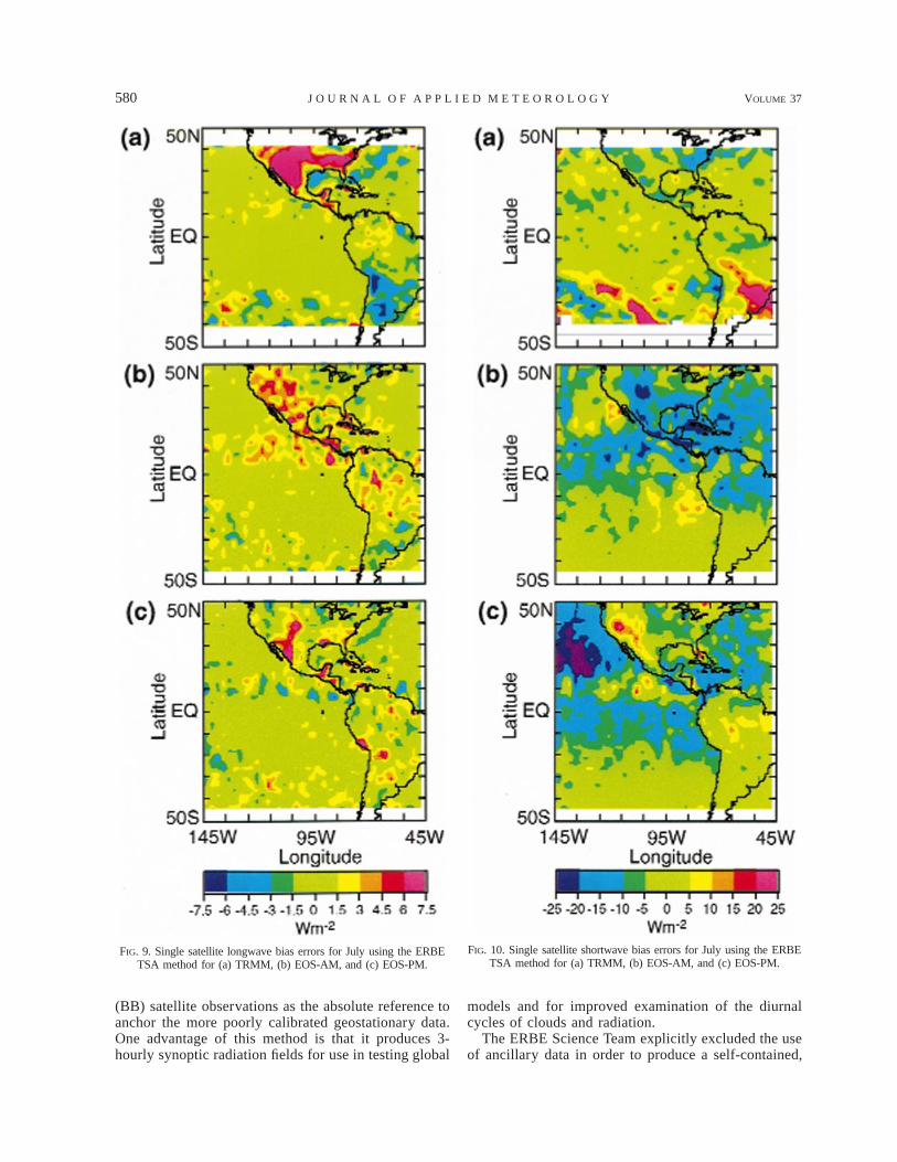
The single satellite bias errors for TRMM, EOS-AM,and EOS-PM are shown in Figs. 9 and 10 for LW andSW, respectively. A TRMM initial equatorial crossing timeof noon (1200) was used for this example, but crossingtimes of 0000, 0600, and 1800 LST were also simulatedto cover the range of sampling that can occur with theprecessing satellite. The TRMM satellite precesses throughall local hours at the equator in about 23 days; thus, sam-pling errors arising from systematic diurnal variations maybe averaged out at low latitudes. Local time coverage ofthe higher latitudes (greater than 308) is not as complete(see Fig. 1). TRMM(12) has positive LW bias errors upto 7 W m22 over much of the United States and Mexico,and similarly large negative errors over South America atlatitudes south of 208S. The location and magnitude ofTRMM errors are also dependent on the satellite crossingtime since different synoptic events may be sampled dif-ferently or entirely missed. For example, TRMM(00), notshown, has maximum positive errors over southern SouthAmerica and large negative errors over North America.The LW errors are generally small over the oceans sincelow-level clouds tend to predominate. The LW samplingerrors for EOS-AM and EOS-PM are also shown in Fig.9. Each of the EOS orbits samples most regions within 2h of noon and midnight, which captures the diurnal vari-ations fairly well. There are notable exceptions in the west-ern United States, in other scattered land regions, and inconvection areas associated with the intertropical conver-gence zone (ITCZ) in the Pacific Ocean near 108N.

Shortwave bias errors for the single satellites are giv-en in Fig. 10. TRMM(12) has errors up to 25 W m22

over both land and ocean regions due to the diurnalvariations of cloud cover. The largest TRMM(12) errorsare primarily located in the southern midlatitudes, whileTRMM(00), not shown, has its greatest errors over a


FIG. 8. GOES July 1985 reference (a) longwave and (b) shortwave data for ERB sampling studies.

large area between 208 and 408N. EOS-AM and EOS-PM have SW bias errors of similar magnitude, but higherrors are seen over a greater geographical area, mainlyin the summer hemisphere.

For multiple satellites, the sampling times of the twoindividual satellites are simply combined before apply-ing the ERBE-like TSA. Results for the two- and three-satellite combinations are given in Figs. 11 and 12 forLW and SW, respectively. The EOS–TRMM combi-nations use the TRMM(12) sampling; slightly differentresults can be expected for the other TRMM orbits. Inevery case, the two-satellite sampling error in themonthly mean is less than that of the single satellites.The combination of all three satellites reduces the erroreven more. Table 1 summarizes both the bias and rmserrors for July and April 1985. The LW mean bias andrms errors are for land regions only, while SW errorsare for the entire study region. For each case that in-cludes a TRMM satellite, the range of values is givenfor all four TRMM starting times. For July 1985 (Table1a), the magnitude of LW bias errors is less than 2 Wm22. The LW rms error is from 3.9 to 5.0 W m22 forTRMM; EOS-AM and EOS-PM errors are 2.9 and 2.6W m22, respectively. Adding a second satellite reducesthe rms error to 2.4 W m22 or less, and the three-satellitecombination error is smaller, 1.3–1.7 W m22.

In general, SW bias errors are somewhat greater thantheir LW counterparts. TRMM SW bias errors range from21.7 to 3.1 W m22, while the EOS satellite SW bias isabout 26 W m22. Adding a TRMM spacecraft to each of

the EOS satellites decreases the bias to about 23.0 Wm22; however, the combination of two EOS orbiters doesnot reduce the SW bias error. The three-satellite case biaserrors vary from 23.4 to 24.0 W m22, similar to thosefor TRMM and one EOS satellite. The rms errors are about10 W m22 for single satellites, slightly less than 6 W m22

for EOS plus TRMM cases, 7.8 W m22 for the combinationof two EOS satellites, and 4.9–5.4 W m22 for the three-satellite case. For April 1985 (Table 1b), the bias and rmserrors are generally smaller than for July; however, thetrend of decreasing errors with an increasing number ofsatellites is essentially the same.

In summary, the ERBE time–space averaging algo-rithm gives regional monthly mean temporal samplingerrors that are significantly reduced as more satellitesare added. Satellites can fail prematurely; therefore, itis useful to provide a strategy to reduce time samplingerrors, especially for the single satellite case. TheTRMM satellite will be in orbit for a year before thelaunch of the first EOS satellite.

3. Method II: Geostationary-data-enhancedtemporal interpolation

Method II incorporates 3-hourly geostationary radi-ance data to account for insufficiently sampled diurnalcycles. The key to this strategy is to use the narrowband(NB) geostationary data to assist in determining theshape of the diurnal cycle, but use the ERB broadband


FIG. 9. Single satellite longwave bias errors for July using the ERBETSA method for (a) TRMM, (b) EOS-AM, and (c) EOS-PM.

FIG. 10. Single satellite shortwave bias errors for July using the ERBETSA method for (a) TRMM, (b) EOS-AM, and (c) EOS-PM.

(BB) satellite observations as the absolute reference toanchor the more poorly calibrated geostationary data.One advantage of this method is that it produces 3-hourly synoptic radiation fields for use in testing global

models and for improved examination of the diurnalcycles of clouds and radiation.

The ERBE Science Team explicitly excluded the useof ancillary data in order to produce a self-contained,


FIG. 11. Multiple satellite longwave bias errors for July using the ERBE TSA method for (a) EOS-AM 1 TRMM, (b) EOS-PM 1 TRMM, (c)EOS-AM 1 EOS-PM, and (d) EOS-AM 1 EOS-PM 1 TRMM.

consistent, and relatively straightforward climate datasetspecifically geared toward accurate measures of monthlymean TOA fluxes. Significant improvements in time in-terpolation could be realized by using ancillary data toprovide additional information concerning the meteo-rological changes occurring between ERB measure-ments.

Numerous simulations were performed to exploretechniques for incorporating additional data sources intothe time-averaging process. Because the main require-ment of such data is to have enhanced temporal reso-lution, an obvious candidate data source is geostationaryand polar-orbiting satellite radiance measurements. Ge-ostationary data from such satellites as GOES, Meteo-sat, INSAT, and Geostationary Meteorological Satellite(GMS) provide measurements of NB visible and infra-

red radiances for much of the globe (approximately508N–508S) at a temporal resolution as fine as every 30min. The polar-orbiting satellites provide much less tem-poral information but are useful for providing infor-mation at higher latitudes.

Many attempts have been made to derive broadbandradiation budget parameters from these narrowband mea-surements (Briegleb and Ramanathan 1982; Doelling etal. 1990; Minnis et al. 1991; Cheruy et al. 1991) becauseof the excellent temporal resolution of geostationary data.Generally, these and other studies (e.g., Gruber et al. 1994)have demonstrated that the narrowband measurements areinsufficient for radiation budget calculations since theymiss valuable spectral information contained in broadbandobservations. Minnis et al. (1991) showed that the long-wave NB–BB relation varied significantly in time and


FIG. 12. Multiple satellite shortwave bias errors for July using the ERBE TSA method for (a) EOS-AM 1 TRMM, (b) EOS-PM 1 TRMM, (c)EOS-AM 1 EOS-PM, and (d) EOS-AM 1 EOS-PM 1 TRMM.

space even when water vapor, surface type, and cloud datawere considered. Figure 13 shows regional means andstandard deviations of the differences between ERBE-mea-sured LW fluxes and broadband LW fluxes derived fromGOES narrowband measurements for April 1985 using aglobal correlation that includes an atmospheric water vaporterm. The overall rms error of the fit is approximately 11W m22, and mean biases greater than 15 W m22 are evidentin many regions over the southeastern Pacific Ocean, overColombia, and off the western coast of Mexico. The great-est standard deviations occur over the U.S.–Mexican bor-der, the Amazon Basin, and the south-central Pacific. Re-gressions performed on a region-by-region basis can re-duce the relative error to 7.7 W m22 and essentially elim-inate the mean bias. However, these regional correlationsrequire frequent updating to account for changes in cali-bration and seasonal variations in the NB–BB relation.

Thus, narrowband data should be used in climate studiesonly if the NB–BB relationship is continually calibratedusing coincident measurements with a broadband ERBinstrument. The techniques that produce the most accurateaverages are described below.

a. Time interpolation of total-sky TOA LW flux

Instead of the combination of linear interpolation andidealized half-sine curves used by the ERBE-like tech-nique to fit the observations, this method uses narrow-band data to provide a more accurate picture of the shapeof the curve that is fit to the observations.

The first step in the process is the conversion of thenarrowband radiances into broadband fluxes using theregression techniques developed by Minnis et al. (1991).The regression is derived from coincident calibrated ge-


TABLE 1. Monthly error summary for ERBE-like diurnal averaging.

Satellite

Longwave (land only)

Bias error(W m22)

rms error(W m22)

Shortwave (all regions)

Bias error(W m22)

rms error(W m22)

(a) July 1985TRMMEOS-AMEOS-PMEOS-AM 1 TRMMEOS-PM 1 TRMMEOS-AM 1 EOS-PMEOS-AM 1 EOS-PM 1 TRMM

21.8–1.01.30.9

0.0–0.820.2–0.5

0.60.2–0.6

3.9–5.02.92.6

2.0–2.41.5–2.2

1.91.3–1.7

21.7–3.126.025.9

23.4–22.423.3–22.8

26.124.0–23.4

8.2–11.19.79.6

5.0–6.05.5–6.0

7.84.9–5.4

(b) April 1985TRMMEOS-AMEOS-PMEOS-AM 1 TRMMEOS-PM 1 TRMMEOS-AM 1 EOS-PMEOS-AM 1 EOS-PM 1 TRMM

21.4–1.10.90.4

0.2–0.520.1–0.1

0.10.1

2.3–5.52.72.3

1.5–1.81.5–1.8

1.71.1–1.2

20.9–1.220.521.820.1

21.0–20.521.2

20.7–20.5

8.4–11.16.45.7

3.7–4.33.6–4.0

3.62.6–2.8

FIG. 13. (a) Regional means and (b) standard deviations of the differences between ERBE-measured LW fluxes and broadband fluxes derivedfrom GOES narrowband measurements for April 1985.

ostationary and ERB measurements and ancillary rel-ative humidity data. The form of the regression is

FFNB 5 a0 1 a1FNB 1 a2 1 a3FNB ln(rh),2FNB (8)

where FFNB is the LW broadband flux derived from thenarrowband, FNB is the narrowband flux, rh is the col-umn-averaged relative humidity, and ai are the derivedcoefficients. The LW narrowband flux is derived fromthe narrowband radiance using

FNB 5 6.18g(u)INB, (9)

where INB is the LW narrowband radiance, g(u) is theLW limb-darkening function at viewing zenith angle u,and 6.18 represents the product of the limb-darkeningfunction integrated over an entire hemisphere and thenarrowband spectral interval (Minnis et al. 1991).

To account for temporal variability in the regressions,new coefficients are derived for each month using data


FIG. 14. Time series of ERBE ERBS (filled squares) and NOAA-9(open circles) LW flux observations and interpolated values from July1985 over New Mexico. The NOAA-9 data are interpolated to other hoursand compared to the observed values from ERBS. The solid curve showsERBE time interpolation values; the dashed line shows the geostationary-data-enhanced interpolation.

from all regions in the satellite field of view. Separatecorrelations are derived for each of the five ERBE geo-graphical scene types. The derivation of separate re-gressions for individual regions in order to account forspatial variability is not feasible for CERES. This isaccomplished instead by normalizing the broadbandfluxes derived from the narrowband data to the mostrecently observed LW measurement.

Once an estimate of broadband flux has been madefrom each narrowband measurement, a complete seriesof FFNB is constructed by using the ERBE-like inter-polation technique. A normalization ratio, «, is then de-fined at the time of each LW measurement during themonth:

F (t )BB 0«(t ) 5 , (10)0 F (t )FNB 0

where t0 is the time of the LW broadband measurement,FFNB is the LW from narrowband after global regression,and FBB is the longwave BB measurement. This ratio islinearly interpolated to all hours of the month. Finalvalues of FBB for all hours between the observations arecalculated by multiplying FFNB by the normalization ra-tio « for that hour. Although there may be some spatialmismatch in the ratioed NB and BB data, this renor-malization is sufficient to reduce the residual regionalvariance from the NB–BB regression. The LW nor-malization process ensures that the final diurnal vari-ability assumed in the time interpolation process is di-rectly tied to the measured fluxes. Errors incurred byvariations in the calibration of the narrowband instru-ments are also reduced. The narrowband data are usedto provide extra information concerning meteorologicalvariations between the measurements. As more than oneERB instrument becomes operational, the reliance onthe narrowband data to provide the diurnal shape willdiminish. With the improved time sampling, the inter-polated curves will be dominated by the observed flux-es.

Several studies have been performed to demonstratethe benefits of incorporating narrowband measurementsinto the averaging process. Past studies have shown thatthe use of techniques, such as the half-sine fit used byERBE over land regions, is more effective than linearinterpolation in reproducing the LW diurnal variabilityseen in narrowband measurements (Brooks and Minnis1984a). Studies such as these rely on using 1-hourlyGOES data converted to broadband flux using NB–BBregressions as a reference dataset. The effects of sam-pling patterns and the relative errors inherent to variousinterpolation schemes can be evaluated by sampling thisreference set and comparing the results of the interpo-lation with the reference set.

To show the improvement in interpolation using thisgeostationary-data-enhanced method, it is necessary tohave three independent datasets: the broadband mea-surements, the narrowband time series, and an additional

broadband reference dataset. Since the GOES data areused in the averaging process, it is improper to useGOES as the reference dataset. In addition, there is no1-hourly global broadband dataset to use as the truth.

This problem is overcome by using ERBE data fromtwo different satellites, ERBS and NOAA-9, as two in-dependent datasets. Observations from one satellite areinterpolated to the observation times of the other usingfour different techniques (denoted as techniques a–d).Technique a is the ERBE-like combination of linear andhalf-sine interpolation. Techniques b, c, and d are ge-ostationary-data-enhanced methods. The first, b, uses 1-hourly GOES data as a best-case test. The second tech-nique, c, uses the 3-hourly time sampling that is mostlikely to be available during CERES processing. Finally,in technique d, ERBE measurements are predicted sim-ply using the 3-hourly narrowband measurements con-verted to broadband using the regression fit but withoutthe normalization to ERBE to account for regional vari-ations. This method is included to determine the needfor continually anchoring the narrowband-derived fluxesto the measurements.

A comparison of two of these techniques, a and c, isdisplayed in Fig. 14 for an ERBE 2.58 region over NewMexico during the first 15 days of July 1985. The solidcurve represents the ERBE-like technique a, while thedashed line is the normalized 3-hourly narrowbandshapes technique c. ERBS observations of TOA LWflux are displayed as solid squares and NOAA-9 obser-vations are open circles. The interpolation techniquesare applied to the NOAA-9 data in order to predict theERBS observations. Both techniques perform well whensampling is adequate and cloudiness is constant as foundduring days 6–8 and 10–12. However, the ERBE TSAseverely misses several nighttime points during days 1–3, as well as daytime points on days 6 and 14. Techniquec does a much improved job of filling in the fluxes inthe hours between the observations. In particular, thepredicted daytime fluxes on day 5 and the nighttimefluxes on days 1–4 are closer to the ERBS values. Afew ERBS fluxes were missed because of the 3-h time


FIG. 15. Regional comparison of instantaneous longwave interpolation errors for (a) ERBE-like and (b) geostationary-data-enhanced time interpo-lation methods for July 1985.

TABLE 2. Comparison of LW flux time interpolation techniquesusing ERBE data from (a) July 1985 and (b) April 1985. Instantaneousmean and rms differences (W m22) between NOAA-9 LW flux mea-surements and fluxes predicted from ERBS observations.

NOAA-9mean flux

Total error

mean rms

Timeinterpolation

error

mean rms

(a) July 1985Coincident dataa: ERBE TSAb: With 1-hourly GOESc: With 3-hourly GOESd: Nonnormalized/3 h

243.6246.5246.5246.5246.5

2.42.83.12.82.6

10.616.911.412.014.4

—0.40.70.40.2

—13.2

4.25.69.7

(b) April 1985Coincident dataa: ERBE TSAb: With 1-hourly GOESc: With 3-hourly GOESd: Nonnormalized/3 h

246.6246.2246.2246.2246.2

20.10.70.80.70.2

10.015.711.311.814.9

—0.80.80.70.2

—12.1

5.36.3

11.0

resolution of the narrowband data, but, overall, tech-nique c shows substantial improvement over technique a.

Figure 15 compares the geographical distribution ofthe LW rms interpolation errors for the ERBE-like (leftpanel) and geostationary-data-enhanced (right panel)temporal interpolation methods for July 1985. Tech-nique c reduced the ERBE mean instantaneous inter-polation rms errors by 50% for both LW and SW (notshown). The greatest improvement using the CEREStechnique occurs in regions with pronounced diurnal

cycles in clouds such as the ITCZ and the convectiveregions of North and South America.

The results for the four interpolation techniques aresummarized in Table 2 for all 2.58 regions between508N–458S latitude and 1558–558W longitude during themonth of July 1985 and between 508N–458S latitudeand 1458–458W longitude during April 1985. The firstrow of the table contains a comparison of coincidentERBS and NOAA-9 ERBE observations. Data from allregions viewed by both ERBE instruments during thesame hour are included. Since this comparison is per-formed using data averaged in coincident hour boxes,any difference between the two can be due to a com-bination of temporal and spatial variations within the2.58 region over 1 h as well as miscalibration betweenthe two instruments or errors in the ADMs used to con-vert the radiances to fluxes. There is a 2.4 W m22 biasand 10.6 W m22 instantaneous rms error (difference)between the two datasets in July. The April data showsimilar values of 20.1 6 10.0 W m22. An estimate canbe made of the magnitude of the errors due to the ADMs.When the two instruments view the scene with viewingzenith angles within 108 of each other, the rms differ-ences are reduced to 5–6 W m22 for both months, whilethe biases remain unchanged.

Although the overall NOAA-9–ERBS biases are small(less than 1% of the mean flux), they are significant tothis study. The results of the various time interpolationschemes must be compared with these coincident biases.A perfect time interpolation should not produce a zero


bias, but rather should reproduce the bias in the coin-cident ERBS and NOAA-9 data.

The successive rows of Table 2 show the capabilityof each interpolation technique to reproduce the NOAA-9 observations by temporally interpolating the ERBSdata. The mean LW flux from NOAA-9 is provided incolumn 1. The next two columns contain the absoluteinstantaneous mean and rms difference between the ob-served NOAA-9 flux and the flux predicted for that hourby interpolating the ERBS observations. Estimates ofthe mean and rms error from the time interpolation pro-cesses have also been included in columns 4 and 5. Therms due to time interpolation, , is calculated as-rmsti

suming that the time interpolation error is independentof the rms difference between coincident ERBS andNOAA-9 measurements, rms0. It is calculated as

5 2 ,2 2 2rms rms rmst T 0i(11)

where rmsT is the total rms from the technique. Themean time interpolation error is simply the differenceof the total mean error and the mean difference in thecoincident fluxes.

The lowest rms errors are obtained using narrowbanddata with 1-h temporal resolution. However, there isonly a slight overall (1–2 W m22) degradation in therms error when 3-hourly data are used. Although thisdegradation is somewhat greater in certain cloud re-gimes, there is a substantial improvement in the timeinterpolation error using the GOES data over the ERBEtime-averaging scheme. The rms error due to time in-terpolation decreases from 13.2 to only 5.6 W m22 forthe July data and from 12.1 to 6.3 W m22 for April. Inaddition, the mean bias is less than 1 W m22 for allcases.

Clearly, the renormalization process is necessary foraccurate temporal interpolation. Technique d simplyused the global NB–BB correlations to produce the LWflux time series from the GOES data. Compared to tech-nique c, it increases the instantaneous time interpolationrms error from 5.6 to 9.7 W m22 in July and from 6.3to 11.0 W m22 in April. The latter error is only a minimalimprovement over the ERBE-like technique a. Throughrenormalization, the time series of LW flux is accuratelytied to the original observations. Region-to-region vari-ations in the NB–BB correlations and temporal varia-tions in the narrowband calibration are explicitly takeninto account.

The statistics from the above simulations show thatthe geostationary-data-enhanced technique improves theinstantaneous flux estimates. It is also crucial that thetime interpolation technique for instantaneous flux doesnot adversely affect the monthly means. Harrison et al.(1990) demonstrated that ERBE regional monthly meanLW flux estimates are accurate within 1 W m22 if datafrom two satellites are used. For July, over the entireGOES region, the ERBE technique a produces monthlymean flux averaged over all regions of 249.0 W m22.For techniques c and d, the averages are 248.8 and 248.4

W m22, respectively. In all three cases, the rms of theregional time interpolation error in the monthly meanis less than 2 W m22. Thus, the enhancements to theinterpolation process are not adversely affecting themonthly means. Once again, the anchoring of the LWfluxes to the observations in technique c produces animprovement over the results of technique d.

Sampling effects are also minimized when narrow-band data are used in the interpolations. The differencesin regional monthly mean fluxes calculated using thetwo ERBE instruments demonstrate the sampling im-pact. The polar-orbiting NOAA-9 satellite producesERBE sampling near 0230 and 1430 LST throughoutthe month. The local time of observations from the pre-cessing ERBS satellite slowly changes during themonth. The region-to-region rms difference between themonthly mean estimates from the two satellites is ameasure of independence of the interpolation from sam-pling effects. During April, when the mean differencebetween the two datasets is nearly zero, the regional rmsdifference in monthly mean is 2.4 W m22 for techniquea and 1.7 W m22 for technique c. As expected, incor-porating the narrowband data time series increased theaccuracy of filling in flux values for times between mea-surements.

b. Time interpolation of clear-sky TOA LW flux

The ERBE-like averaging technique does not yieldclear-sky flux estimates for all hours of the month. Therelative scarcity of clear-sky flux estimates derived fromERBE data necessitated the use of monthly–hourly fitsinstead of continuous interpolation. CERES is gearedtoward studying the effects of clouds on the earth’s ra-diation budget, so there will be a significant improve-ment in the quality of clear-sky data. The frequency ofclear scenes misclassified as partly cloudy will be sub-stantially reduced.

Because of these improvements to the clear-sky da-taset, time interpolation of clear-sky LW flux is per-formed in a manner identical to the total-sky product.The main information provided by the narrowband ge-ostationary data relates to changes in meteorology andcloudiness. For clear skies, the idealized ERBE modelswork well. If no clear-sky measurements are availableon a given day, clear-sky fits from the nearest day withdata is used.

c. Time interpolation of total-sky TOA SW flux

There are several major challenges that must be ad-dressed when developing a method of incorporating nar-rowband data into the process of temporal interpolationof TOA SW fluxes. First, in order to calculate a nar-rowband albedo, anisotropic effects must be removedthrough the use of bidirectional reflectance models.Since these models are functions of both surface typeand cloud cover, it is important to have accurate esti-


mates of the cloud amount at the times of the narrow-band observations. Second, the narrowband albedosmust be converted into equivalent broadband values. Aswith the TOA LW flux, a normalization process is usedto ensure that the resulting time series of albedos is tiedto the broadband observations.

Two methods are used to determine broadband albedofrom narrowband reflectances. The first method (re-ferred to as the GOES cloud method) uses cloud infor-mation derived from the narrowband data. For thisstudy, the cloud parameters were derived using the Hy-brid Bispectral Threshold Method (HBTM) of Minniset al. (1987). Each narrowband pixel is classified aseither clear or cloudy. For each region, these pixels canbe averaged to produce the cloud amount (cld) and sep-arate estimates of clear sky (rclr) and overcast (rcld) re-flectance. Narrowband albedo, anb, can then be com-puted from rclr and rcld using

(1.0 2 cld)(r ) (cld)(r )clr clda 5 1 , (12)nb R Rclr ovc

where r is narrowband reflectance (r 5 Inb/Sy ), cld isthe narrowband cloud amount, and R is the bidirectionalanisotropic factor. Here, Inb is the mean observed nar-rowband VIS radiance and Sy is the earth–sun distance-corrected narrowband solar constant (nominal value forGOES of 526.9 W m22 sr21 mm21).

The second method (referred to as the ERBE cloudmethod) assumes that no cloud information is derivedfrom narrowband data. The only available cloud infor-mation is the scene fractions of the four ERBE cloudclassifications measured at the times of the broadbandobservations. Cloud amount at the time of the narrow-band measurement is estimated by linearly interpolatingthese scene fractions. However, there is still insufficientinformation to calculate narrowband albedos since thereare not separate estimates of reflectance for each cloudclassification. A composite bidirectional anisotropic fac-tor can be calculated by weighting the individual factorsby both the scene fraction and the relative amount ofenergy reflected by each cloud classification. To do this,initial estimates of albedo (ai) are calculated at the nar-rowband times by using the ERBE interpolation tech-nique described in Eq. (4). The narrowband radiancescan then be converted to narrowband albedos using

4 4

a 5 (I /S ) R a f a f , (13)O Onb nb y i i i i i@1 @ 2i51 i51

where f i and Ri are the ERBE scene fraction and bi-directional anisotropic factors for ADM class i inter-polated to the time of the narrowband data.

Broadband anisotropic factors have been used in theabove calculation. Doelling et al. (1990) showed thatthe use of ERBE broadband anisotropic factors in thecalculation of albedos from GOES measurements didnot degrade the regressions between GOES and ERBEalbedos.

For both the GOES and ERBE cloud methods, thenarrowband albedos are converted to estimates of broad-band albedos using regressions of the form used byDoelling et al. (1990),

aBB 5 b0 1 b1aNB 1 b2 1 b3 ln[sec(u0)], (14)2aNB

where aNB is the narrowband albedo, aBB is the broad-band albedo estimate from the narrowband data, and u0

is the solar zenith angle at the center of the region atthe synoptic time. Separate regressions have been per-formed for each of the five ERBE geographical scenetypes.

A time series of broadband albedos calculated fromnarrowband measurements in the above manner can stillcontain significant errors (see Doelling et al. 1990; Brie-gleb and Ramanathan 1982). Doelling et al. (1990)found that regressions of the form in (14) have rmsregression errors in excess of 14%. In addition, theyshowed that the relationship can vary substantially fromregion to region. The best measurements of broadbandSW flux are those derived from broadband ERB instru-ments. Like the LW methods, the time series of nar-rowband measurements should serve only as a guidefor tracking changes in cloudiness between the ERBobservation times. This can be significant since varia-tions in cloudiness have a much greater impact on theSW. A change from a 100% clear scene to 100% over-cast may result in a decrease in LW flux of 20%–30%,but total-scene albedo may increase by 400%–500%.

As with the LW, the derived albedos are normalizedto the broadband observations. At each SW observationtime, a normalization ratio can be defined as the ratioof the observed albedo to aBB. This ratio can then beinterpolated to all daylight hours and used to normalizeeach estimate of aBB. However, it has been found thatdue to the large variation of albedo with cloud amount,normalization at all hours can produce albedos outsideof physical limits; constraints need to be determined inorder to normalize more hour boxes. For this study,albedos are normalized only for a 2-h window surround-ing each SW measurement. Because of the variabilityof the SW narrowband–broadband relationship, eventhis limited normalization process produces a more ac-curate interpolation.

The accuracy of these techniques was tested usingERBE ERBS and NOAA-9 SW data. Measurementsfrom ERBS were used to predict SW flux values mea-sured from NOAA-9 using five techniques. Technique auses the ERBE method. The other techniques employnarrowband SW radiances from GOES. The differencebetween the techniques is in the cloud data used to selectthe ADMs necessary to convert the narrowband radi-ances into fluxes. The interpolation is first performedusing cloud amounts and cloud and clear albedos de-rived from the narrowband data using HBTM (Minniset al. 1987). The results from this technique representbest-case examples and are labeled b and c when appliedto 1-hourly and 3-hourly GOES data, respectively. The


TABLE 3. Comparison of SW flux time interpolation techniques using ERBE data from (a) July 1985 and (b) April 1985. Instantaneousmean and rms differences (W m22) between NOAA-9 SW flux measurements and fluxes predicted from ERBS observations.

NOAA-9mean flux

Total error

mean rms

Time interpolation error

mean rms

(a) July 1985Coincident dataa: ERBE TSAb: With 1-hourly GOES 1 GOES cloudsc: With 3-hourly GOES 1 GOES cloudsd: With 1-hourly GOES 1 ERBE cloudse: With 3-hourly GOES 1 ERBE cloudsf: Nonnormalized 3 h 1 ERBE clouds

259.4228.5228.5228.5228.5228.5228.5

5.20.0

21.020.8

6.25.97.1

36.553.835.136.039.539.642.5

—24.625.625.4

1.61.42.5

—43.114.116.222.923.127.8

(b) April 1985Coincident dataa: ERBE TSAb: With 1-hourly GOES 1 GOES cloudsc: With 3-hourly GOES 1 GOES cloudsd: With 1-hourly GOES 1 ERBE cloudse: With 3-hourly GOES 1 ERBE cloudsf: Nonnormalized 3 h 1 ERBE clouds

251.0233.3233.3233.3233.3233.3233.3

5.11.75.73.45.23.23.1

39.155.137.138.539.942.444.9

—23.0

1.021.3

0.421.521.6

—41.4

7.512.716.521.826.4

next two techniques, d and e, use linearly interpolatedERBE cloud amounts and albedos to select the properanisotropic factor. Technique d uses 1-hourly GOESdata; technique e uses 3-hourly data. A final technique,f, is identical to e, but it does not include the renor-malization of the narrowband-derived fluxes to the near-est observation.

The results are shown in Table 3. There is a significantbias between coincident ERBS and NOAA-9 measure-ments. During both July and April, the instantaneousmean differences are approximately 5.2 W m22 withapproximately 38 W m22 rms. These differences aremuch larger than the corresponding values associatedwith the LW flux. This is due to the greater dependenceon ADMs for deriving SW flux from the observations.When the coincident comparison is limited to timeswhen both instruments are viewing within 208 of nadir,the mean bias in July is 21.4 W m22 and the rms dif-ference falls to only 13.1 W m22, which is of the samemagnitude as the LW. Unfortunately, the additional er-rors associated with model selection hamper some ofthe comparisons in the simulations. Since the mean dif-ferences of even coincident data are strongly angle de-pendent, it is difficult to determine the absolute accuracyof the averaging techniques. However, the relative ef-fectiveness of the methods can be measured by com-paring the rms errors. Thus, analysis of the simulationswill stress a comparison of the instantaneous rms errors,not the biases.

The mean and rms errors due to time interpolationare calculated in a slightly different fashion than thatused for the LW flux simulations. As seen in Table 3,the mean SW flux for the coincident data is 20–30 Wm22 greater than the mean fluxes used in the time in-terpolation. There are fewer (approximately 7000) co-incident data points as compared with the approximately35 000 NOAA-9 measurements that can be predicted

from ERBS data. The difference in the mean fluxesoccurs because the coincident data occur at a loweraverage solar zenith angle. To accommodate this dif-ference, the rms errors from the coincident data [rms0

from (11)] are first linearly scaled by the ratio of thefluxes before being subtracted from the total rms errors.

The addition of narrowband data significantly de-creases the interpolation rms errors. As explained above,the ERBE time interpolation technique necessarily as-sumes constant cloudiness over each day for which thereis only one time of observation. By introducing infor-mation concerning the temporal variation in cloudinessthrough the addition of narrowband data, the time in-terpolation error has been reduced from 43.1 W m22 toless than 28 W m22 in all cases b–f for the July data.The reasons for this increased accuracy can be seen inFig. 16, which shows 3 days of SW albedo measuredby ERBE during July 1985 in the same region in NewMexico as in Fig. 14. The ERBS observations are shownas black squares. The NOAA-9 observations are opencircles. Also shown are the results of interpolations us-ing the NOAA-9 data and the ERBE time interpolationtechnique a and the 3-hourly geostationary data tech-nique e. During the first two days, the cloudiness re-mained constant throughout the day and the two tech-niques produce similar results. On the third day, how-ever, there was apparently a shift in cloudiness betweenERBS and NOAA-9 observation times. The ERBE timeinterpolation technique severely overestimates the al-bedo over most of the day. The GOES data, however,provide the means for correctly modeling the albedo onthat day.

Technique e provides a definite improvement over theERBE technique, reducing the rms time interpolationerror from 43.1 to 23.1 W m22 in July and from 41.4to 21.8 W m22 in April. The bias errors also show im-provement. As expected, the mean rms error associated


FIG. 16. Time series of ERBE ERBS (filled squares) and NOAA-9(open circles) SW albedo observations and interpolated values from July1985 over New Mexico. The solid curve shows the ERBE time inter-polated values; the dashed curve shows the geostationary-data-enhancedinterpolation.

with using 1-hourly data in technique d shows a slightimprovement over using 3-hourly data. However, thisimprovement is small compared to the advantages ofdata volume reduction if 3-hourly data are used instead.Furthermore, when generating SW flux estimates forsynoptic maps, the difference between the 1- and 3-hourly data is not significant. Since the fluxes will bederived at times of geostationary observations, the er-rors should be closer to the 1-hourly estimates shownhere. It is clear in these results that the renormalizationof the SW flux estimates to the nearest observation isimportant. The rms errors increase by 4–5 W m22 whenthis renormalization is not included in technique f.

An additional improvement is seen if cloud infor-mation is derived at the times of geostationary mea-surements. As stated above, errors can be quite largefrom improper selection of SW ADMs due to misclas-sification of cloud amount. Increasing the accuracy ofcloud parameters should, therefore, decrease errors inthe NB–BB conversion of the GOES data. For tech-niques d–f, cloud fraction estimates are derived at eachhour by linearly interpolating between ERBE obser-vations. Cloud fractions derived directly from the nar-rowband data should be more accurate since time in-terpolation of cloud fraction is no longer necessary.

The results of using this improved cloud informationare shown in techniques b and c for 1- and 3-h GOESdata, respectively. For the 3-hourly case, rms interpo-lation errors decrease by 7–9 W m22 from technique e,which uses the ERBE cloud information. Part of thiserror is due to the linear interpolation of cloud fractions,but some of the error is due to incorrect ERBE sceneidentification. This latter error should be greatly dimin-ished because of the improved cloud data from futureERB experiments such as CERES. Thus, the improve-

ment of technique c over e should not be as great forCERES. The actual gain in accuracy using c instead ofe for CERES needs further study.

These new temporal interpolation methods are aimedat improving instantaneous estimates of flux. It is im-portant to ensure that the estimates of monthly meanflux are not adversely affected. ERBE produced regionalmonthly mean SW flux estimates to within 3 W m22

(Harrison et al. 1990). For July, the ERBE method aproduces monthly mean flux averaged over all regionsof 95.1 W m22. For techniques e and f, the averagesare 95.5 and 95.6 W m22, respectively. Thus, the en-hancements to the interpolation process are not adverse-ly affecting the monthly means. Once again, anchoringthe SW fluxes to the observations in technique e pro-duces an improvement over the results of technique f.

d. Time interpolation of clear-sky TOA SW flux

As is the case for the clear-sky LW flux, there shouldbe a more accurate determination of clear-sky SW datawith the CERES experiments than with ERBE. The ERBdata are interpolated using the clear-sky ADMs appro-priate to the regional surface type. Thus, geostationarydata should not be needed for clear-sky modeling. Themain information provided by the narrowband data isthe changes in meteorology and cloudiness. For clearskies, the available directional models should work wellfor time interpolation. Geostationary data could only beused in the processing of clear-sky data if separate total-sky and clear-sky narrowband radiances are derivedfrom the narrowband measurements.

4. Conclusions

Two general methods are presented and evaluated fortemporally interpolating ERB measurements to computeaverages of TOA SW and LW flux. A method similarto that used by the ERBE yields good monthly averages,but it does not always provide an accurate representationof diurnal variations. The new CERES geostationary-data-enhanced technique incorporates high-temporalresolution data from geostationary satellites and reducesthe ERBE-like mean instantaneous interpolation rms er-rors by 50% for both SW and LW. The greatest im-provement using the geostationary-data-enhanced tech-nique occurs in regions with pronounced diurnal cyclesin clouds, such as the ITCZ and the convective regionsof North and South America. While proposed for ap-plication to future earth radiation budget measurementprograms such as CERES, these new techniques mayalso be useful for improving the fluxes derived fromearlier ERB data.

REFERENCES

Barkstrom, B. R., 1984: The Earth Radiation Budget Experiment(ERBE). Bull. Amer. Meteor. Soc., 65, 1170–1185.


, and G. L. Smith, 1986: The Earth Radiation Budget Experiment:Science and implementation. Rev. Geophys., 24, 379–390., E. F. Harrison, R. B. Lee III, and the ERBE Science Team,1990: Earth Radiation Budget Experiment, preliminary seasonalresults. Eos, Trans., Amer. Geophys. Union, 71, 297–305.

Briegleb, B. P., and V. Ramanathan, 1982: Spectral and diurnal vari-ations in clear sky planetary albedo. J. Climate Appl. Meteor.,21, 1168–1171.

Brooks, D. R., and P. Minnis, 1984a: Comparison of longwave diurnalmodels applied to simulations of the Earth Radiation BudgetExperiment. J. Climate Appl. Meteor., 23, 156–160., and , 1984b: Simulation of the earth’s monthly averageregional radiation balance derived from satellite measurements.J. Climate Appl. Meteor., 23, 392–403., E. F. Harrison, P. Minnis, J. T. Suttles, and R. S. Kandel, 1986:Development of algorithms for understanding the temporal andspatial variability of the earth’s radiation balance. Rev. Geophys.,24, 422–438.

Cheruy, F., R. S. Kandel, and J. P. Duvel, 1991: Outgoing longwaveradiation and its diurnal variations from combined Earth Radi-ation Budget Experiment and Meteosat observations, 2, UsingMeteosat data to determine the longwave diurnal cycle. J. Geo-phys. Res., 96, 22 623–22 630.

Doelling, D. R., D. F. Young, R. F. Arduini, P. Minnis, E. F. Harrison,and J. T. Suttles, 1990: On the role of satellite-measured nar-rowband radiances for computing the earth’s radiation balance.Preprints, Seventh Conf. on Atmospheric Radiation, San Fran-cisco, CA, Amer. Meteor. Soc., 155–160.

Gruber, A., and J. S. Winston, 1978: Earth–atmosphere radiative heat-ing based on NOAA scanning radiometer measurements. Bull.Amer. Meteor. Soc., 59, 1570–1573., R. Ellingson, P. Ardanuy, M. Weiss, S.-K. Yang, and S. N. Oh,1994: A comparison of ERBE and AVHRR longwave flux es-timates. Bull. Amer. Meteor. Soc., 75, 2115–2130.

Harrison, E. F., P. Minnis, and G. G. Gibson, 1983: Orbital and cloudcover sampling analyses for multisatellite earth radiation budgetexperiments. J. Spacecraft Rockets, 20, 491–495., and Coauthors, 1988: First estimates of the diurnal variationof longwave radiation from the multiple-satellite Earth RadiationBudget Experiment (ERBE). Bull. Amer. Meteor. Soc., 69, 1144–1151.

, P. Minnis, B. R. Barkstrom, B. A. Wielicki, G. G. Gibson, F.M. Denn, and D. F. Young, 1990: Seasonal variation of the di-urnal cycles of earth’s radiation budget determined from ERBE.Preprints, Seventh Conf. on Atmospheric Radiation, San Fran-cisco, CA, Amer. Meteor. Soc., 87–91.

Hartmann, D. L., K. J. Kowalewsky, and M. L. Michelsen, 1991:Diurnal variations of outgoing longwave radiation and albedofrom ERBE scanner data. J. Climate, 4, 598–617.

Jacobowitz, H., W. L. Smith, H. B. Howell, and F. W. Nagle, 1979:The first 18 months of planetary radiation budget measurementsfrom the Nimbus-6 ERB experiment. J. Atmos. Sci., 36, 501–507.

Minnis, P., and E. F. Harrison, 1984: Diurnal variability of regionalcloud and clear-sky radiative parameters derived from GOESdata. Part I: Analysis method. J. Climate Appl. Meteor., 23, 993–1011., , and G. G. Gibson, 1987: Cloud cover over the easternequatorial Pacific derived from July 1983 ISCCP data using ahybrid bispectral threshold method. J. Geophys. Res., 92, 4051–4073., D. F. Young, and E. F. Harrison, 1991: Examination of therelationship between outgoing infrared window and total long-wave fluxes using satellite data. J. Climate, 4, 1114–1133.

Raschke, E., and W. R. Bandeen, 1970: The radiation balance of theplanet earth from radiation measurements of the satellite Nimbus-II. J. Climate Appl. Meteor., 9, 215–238., T. H. Vonder Haar, M. Pasternak, and W. R. Bandeen, 1973:The radiation balance of the earth–atmosphere system from Nim-bus-3 radiation measurements. NASA Tech. Note D-7249, 73pp.

Suttles, J. T., and Coauthors, 1988: Angular radiation models forEarth–atmosphere system; Vol. I, Shortwave radiation. NASARP-1184, 144 pp.

Taylor, V. R., and L. L. Stowe, 1984: Reflectance characteristics ofuniform earth and cloud surfaces derived from Nimbus-7 ERB.J. Geophys. Res., 89, 4987–4996.

Wielicki, B. A., and R. N. Green, 1989: Cloud identification for ERBEradiative flux retrieval. J. Appl. Meteor., 28, 1133–1146., B. R. Barkstrom, E. F. Harrison, R. B. Lee, III, G. L. Smith,and J. E. Cooper, 1996: Clouds and the Earth’s Radiant EnergySystem (CERES): An earth observing system experiment. Bull.Amer. Meteor. Soc., 77, 853–868.

temporal interpolation methods for the clouds and the

Documents