temporal-difference learning - tu chemnitz · temporal-difference learning 18 random walk example!...
TRANSCRIPT

Temporal-Difference Learning 0
Temporal-Difference Learning
Suggested reading:
Chapter 6 in R. S. Sutton, A. G. Barto: Reinforcement Learning: An Introduction MIT Press, 1998.
Temporal-Difference Learning 1
Contents:
• TD Prediction
• TD Policy evaluation • Advantages of TD Prediction Methods
• TD vs. MC • Sarsa: On-Policy TD Control
• Q-Learning: Off-Policy TD Control • Actor-critic
• R-learning
Temporal-Difference Learning

Temporal-Difference Learning 2
TD Prediction!
!
Simple every - visit Monte Carlo method :
V (st )" V (st ) +# Rt $V (st )[ ]
Policy Evaluation (the prediction problem): ! for a given policy !, compute the state-value function !
!
V "
Recall:!
!
The simplest TD method, TD(0) :
V (st )" V (st ) +# rt+1 + $V (st+1) %V (st )[ ]
target: the actual return after time t!
target: an estimate of the return!
Temporal-Difference Learning 3
TD Prediction!
TD(0)!
MC!
!
= "(s,a) Ps # s a Rs # s
a + $V " ( # s )[ ]# s %
a% DP!
MC, TD and DP make different estimates of the value function:

Temporal-Difference Learning 4
Simple Monte Carlo!
T! T! T! T!T!
T! T! T! T! T!
T! T!
T! T!
T!T! T!
T! T!T!
!
V (st )" V (st ) +# Rt $V (st )[ ]where Rt is the actual return following state st .
!
st
Monte Carlo uses an estimate of the actual return.
Temporal-Difference Learning 5
Dynamic Programming!
T!
T! T! T!T!
T!T!
T!
T!T!
T!
T!
T!
!
st
!
st+1
!
rt+1!
V (st )" E# rt+1 + $V (st ){ }
The DP target is an estimate not because of the expected values, which are assumed to be completely provided by a model of the environment, but because V! is not known and the current estimate is used instead.

Temporal-Difference Learning 6
Simplest TD Method!
T! T! T! T!T!
T! T! T! T! T!T!T!T!T!T!
T! T! T! T! T!
!
V (st )" V (st ) +# rt+1 + $V (st+1) %V (st )[ ]
!
st
!
st+1
!
rt+1
TD samples the expected value and uses the current estimate of the value.
Temporal-Difference Learning 7
TD(0) - Policy-Evaluation!
„temporal Difference“

Temporal-Difference Learning 8
Example !
d e f
a b c
0 0 0
0 0 0
Initialize
0 0 0
0 0 90 !
c " f
0 0 0
0 0 0
Temporal-Difference Learning 9
Example!
0 0 0
0 0 90
0 0 0
0 0 90
0 90 0
0 0 90
0 0 0
0 0 90

Temporal-Difference Learning 10
Example!
0 90 0
0 81 90
0 90 0
0 0 90
81 90 0
0 81 90
0 90 0
0 81 90
Temporal-Difference Learning 11
Example!
81 90 0
73 81 90
81 90 0
0 81 90
81 90 0
73 81 99
81 90 0
73 81 90

Temporal-Difference Learning 12
Example!
81 99 0
73 81 99
81 90 0
73 81 99
81 99 0
73 81 83
81 99 0
73 81 99
Temporal-Difference Learning 13
Example!
100 100 0
100 100 100
52 66 0
49 57 76

Temporal-Difference Learning 14
TD methods bootstrap and sample!
• Bootstrapping: update uses an estimate of the successor state!– MC does not bootstrap!– DP bootstraps!– TD bootstraps!
• Sampling: update looks ahead for a sample successor state!– MC samples!– DP does not sample!– TD samples!
Temporal-Difference Learning 15
Example: Driving Home!
• The “rewards” are the elapsed times on each leg of the journey.!• We are not discounting (!=1), and thus the return for each state is the
actual time to go from that state.!• The value of each state is the expected time to go.!

Temporal-Difference Learning 16
Driving Home!
road
30
35
40
45
Predictedtotal
traveltime
leavingoffice
exitinghighway
2ndary home arrive
Situation
actual outcome
reachcar street home
Changes recommended by Monte Carlo methods (!=1)!
Changes recommended!by TD methods (!=1)!
!
V (st )" V (st ) +# Rt $V (st )[ ]
!
V (st )" V (st ) +# rt+1 + $V (st+1) %V (st )[ ]
MC must wait with the update until the final outcome!
Temporal-Difference Learning 17
Advantages of TD Prediction Methods!
• TD methods do not require a model of the environment, only experience!
• TD, but not MC, methods can be fully incremental!– You can learn before knowing the final outcome!
• Less memory!• Less peak computation!
– You can learn without the final outcome!• From incomplete sequences!
• Both MC and TD converge (under certain assumptions to be detailed later), but which is faster?!

Temporal-Difference Learning 18
Random Walk Example!
• All episodes start in the center state C!• proceed either left or right by one state on each step, with equal
probability !• Episodes terminate either on the extreme left or the extreme right.!• When an episode terminates on the right a reward of 1 occurs; all
other rewards are zero. !• Because this task is undiscounted and episodic, the true value of
each state is the probability of terminating on the right if starting from that state. !
• The true values of all the states, A through E, are 1/6, 2/6, 3/6, 4/6, 5/6!
Temporal-Difference Learning 19
Random Walk Example!
A B C D E100000
start
Values learned by TD(0) after!various numbers of episodes!

Temporal-Difference Learning 20
TD and MC on the Random Walk!
Data averaged over!100 sequences of episodes!
Temporal-Difference Learning 21
Optimality of TD(0)!
Batch Updating: train completely on a finite amount of data, e.g., train repeatedly on 10 episodes until convergence.!
Compute updates according to TD(0), but only update! estimates after each complete pass through the data. !
For any finite Markov prediction task, under batch updating,!TD(0) converges for sufficiently small α.!
Constant-α MC also converges under these conditions, but to a difference answer! !

Temporal-Difference Learning 22
Random Walk under Batch Updating!
. 0
.05
. 1
.15
. 2
.25
0 25 50 75 100
TDMC
BATCH TRAINING
Walks / Episodes
RMS error,averagedover states
After each new episode, all previous episodes were treated as a batch, and algorithm was trained until convergence. All repeated 100 times.!
?
Temporal-Difference Learning 23
TD vs. MC !
Suppose you observe the following 8 episodes:!
A, 0, B, 0!B, 1!B, 1!B, 1!B, 1!B, 1!B, 1!B, 0!
You are the Predictor:!
This means that the first episode started in state A, transitioned to B with a reward of 0, and then terminated from B with a reward of 0. !
The other seven episodes were even shorter, starting from B and terminating immediately.!
What is the optimal value for the estimate V(A) given this data? !

Temporal-Difference Learning 24
TD vs. MC !
A B
r = 1
100%
75%
25%
r = 0
r = 0
Temporal-Difference Learning 25
TD vs. MC !
• The prediction that best matches the training data is V(A)=0!– This minimizes the mean-square-error on the training set!– This is what a batch Monte Carlo method gets!
• If we consider the sequentiality of the problem, then we would set V(A)=.75!– This is correct for the maximum likelihood estimate of a
Markov model generating the data !– This is called the certainty-equivalence estimate, because it is
equivalent to assuming that the estimate of the underlying process was known with certainty rather than being approximated.!
– This is what TD(0) gets!

Temporal-Difference Learning 26
Sarsa: On-Policy TD Control!
st+2,at+2st+1,at+1
rt+2rt+1st st+1st ,atst+2
!
Estimate Q" for the current behavior policy ".
!
Q st ,at( )" Q st ,at( ) +# rt+1 + $Q st+1,at+1( ) %Q st ,at( )[ ]
If st+1 is terminal, then Q(st+1,at+1) = 0.
Sarsa: Learning An Action-Value Function
!
After every transition from a nonterminal state st , do :
Temporal-Difference Learning 27
Sarsa: On-Policy TD Control!
Turn this into a control method by always updating the!policy to be greedy with respect to the current estimate: !
On-Policy
Quintupel!

Temporal-Difference Learning 28
Sarsa: On-Policy TD Control!
S G
0 0 0 01 1 1 12 2
standardmoves
king'smoves
undiscounted, episodic task with constant rewards reward = –1 until goal
Move from S to G, but consider the crosswind that moves you upward. For example, if you are one cell to the right of the goal, then the action left takes you to the cell just above the goal. !
strength of the wind
Windy Gridworld !
Temporal-Difference Learning 29
Sarsa: On-Policy TD Control!
!
" = 0.1, # = 0.1
Can Monte Carlo methods be used on this task? !
No, since termination is not guaranteed for all policies.!
Step-by-step learning methods (e.g. Sarsa) do not have this problem. They quickly learn during the episode that such policies are poor, and switch to something else.!
And Sarsa? !
Results of Sarsa on the Windy Gridworld!

Temporal-Difference Learning 30
Q-Learning: Off-Policy TD Control!
!
One - step Q - learning :
Q st ,at( )" Q st ,at( ) +# rt+1 + $ maxaQ st+1,a( ) %Q st ,at( )[ ]
Off-Policy
Temporal-Difference Learning 31
Example!
d e f
a b c Initialize
d e f
a b c
d e f
a b c

Temporal-Difference Learning 32
Example!
d e f
a b c
d e f
a b c
d e f
a b c
Temporal-Difference Learning 33
Example!
d e f
a b c
d e f
a b c
81
66 81

Temporal-Difference Learning 34
Example!
c b a
f e d
100
100 90
81 73
90 81 81 73
90
81
81
Temporal-Difference Learning 35
Cliffwalking!
"-greedy, " = 0.1!
Reward is on all transitions -1 except those into the the region marked "The Cliff."
Q-learning learns quickly values for the optimal policy, that which travels right along the edge of the cliff. Unfortunately, this results in its occasionally falling off the cliff because of the "-greedy action selection. Sarsa takes the action selection into account and learns the longer but safer path through the upper part of the grid.
If " were gradually reduced, then both methods would asymptotically converge to the optimal policy.

Temporal-Difference Learning 36
Actor-Critic Methods!
• Explicit representation of policy as well as value function!
• Critic drives all learning!• On policy method!• Appealing as psychological
and neural models !
Policy
TDerror
Environment
ValueFunction
reward
state action
Actor
Critic
Temporal-Difference Learning 37
Actor-Critic Details!
!
" t = rt+1 + #V (st+1) $V (st )
!
p(st ,at )" p(st ,at ) + #$ t
Typically, the critic is a state-value function. After each action selection, the critic evaluates the new state to determine whether things have gone better or worse than expected. That evaluation is the TD error:!
Let’s assume actions are determined by preferences, p(s,a), as follows:!
!
" t (s,a) = Pr at = a st = s{ } =ep(s,a )
ep(s,b )b#
,
Then strengthening or weakening the preferences, p(s,a), depends on the TD error (β – step size parameter):!

Temporal-Difference Learning 38
Actor-Critic Methods!
Advantages:!• Minimal computation to select
actions, since it does not have to search through the action space – particularly important for large action spaces.!
• Can learn an explicit stochastic policy!
Policy
TDerror
Environment
ValueFunction
reward
state action
Actor
Critic
Temporal-Difference Learning 39
R-Learning for Undiscounted Continuing Tasks!
• off-policy control method !• no discounts!• no division of experience into distinct episodes with
finite returns !• one seeks to obtain the maximum reward per time step!
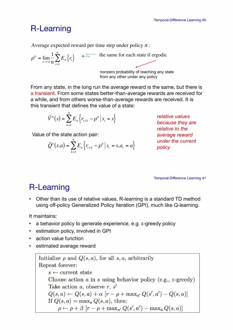
Temporal-Difference Learning 40
R-Learning!
!
Average expected reward per time step under policy " :
#" = limn$%
1n
E" rt{ }t=1
n
& the same for each state if ergodic!
!
˜ Q " s,a( ) = E" rt +k # $" st = s,at = a{ }
k =1
%
&
nonzero probability of reaching any state from any other under any policy
!
˜ V " s( ) = E" rt +k # $" st = s{ }
k =1
%
&
From any state, in the long run the average reward is the same, but there is a transient. From some states better-than-average rewards are received for a while, and from others worse-than-average rewards are received. It is this transient that defines the value of a state: !
Value of the state action pair:!
relative values because they are relative to the average reward under the current policy!
Temporal-Difference Learning 41
R-Learning!• Other than its use of relative values, R-learning is a standard TD method
using off-policy Generalized Policy Iteration (GPI), much like Q-learning.
It maintains:!• a behavior policy to generate experience, e.g. "-greedy policy • estimation policy, involved in GPI • action value function!• estimated average reward!
Temporal-Difference Learning 42
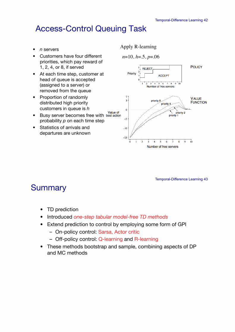
Access-Control Queuing Task!
• n servers!
• Customers have four different priorities, which pay reward of 1, 2, 4, or 8, if served!
• At each time step, customer at head of queue is accepted (assigned to a server) or removed from the queue!
• Proportion of randomly distributed high priority customers in queue is h!
• Busy server becomes free with probability p on each time step!
• Statistics of arrivals and departures are unknown!
n=10, h=.5, p=.06!
Apply R-learning!
Temporal-Difference Learning 43
Summary!
• TD prediction!• Introduced one-step tabular model-free TD methods!• Extend prediction to control by employing some form of GPI!
– On-policy control: Sarsa, Actor critic!– Off-policy control: Q-learning and R-learning!
• These methods bootstrap and sample, combining aspects of DP and MC methods!
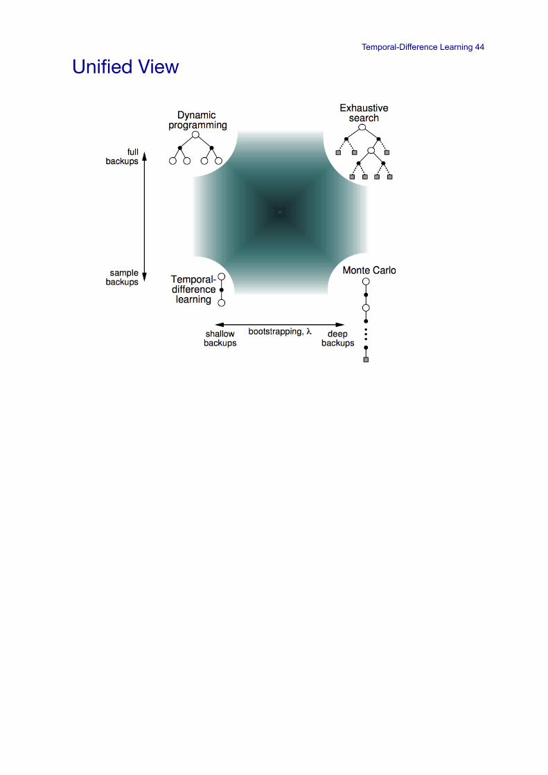
Temporal-Difference Learning 44
44!
Unified View!