Temperature, Test Scores, and Educational Attainment

Jisung Park

Harvard University Economics Department ∗

September 14, 2016

Abstract

How does temperature affect educational attainment? Evidence from 4.6 million

high school exit exams from New York City suggests that heat stress can significantly

diminish exam performance in the short run and reduce educational attainment in the

long run. Taking an exam on a 90◦F day relative to a 72◦F day leads to a 0.19 stan-

dard deviation reduction in performance, equivalent to a quarter of the Black-White

achievement gap, and a 12.3% higher likelihood of failing an exam. Hot days during

the school year reduce subsequent exam performance by 2.2% of a standard deviation

per day above 80◦F, suggesting that cumulative heat exposure can reduce the rate

of learning. This study finds some evidence for protective effects of air conditioning,

and strong evidence for “adaptive grading”, whereby teachers partially offset the ad-

verse performance impacts of acute heat stress by manipulating grades near passing

thresholds when students have experienced hot exam sittings. These findings may

have implications for estimating the social cost of carbon, designing education policy,

and our understanding of the role that climatic factors play in explaining income gaps

across individuals and nations.

∗The author would like to thank Larry Katz, Robert Stavins, Andrei Shleifer, Geoffrey Heal, Raj Chetty,

Joe Aldy, Claudia Goldin, Edward Glaeser, Jim Stock, Martin Feldstein, Jeff Miron, Jeff Liebman, Greg

Mankiw, Josh Goodman, David Keith, Peter Huybers, Daniel Schrag, Max Auffhammer, Sol Hsiang, Sean

Reardon, Olivier Deschenes and numerous seminar participants at Harvard, Columbia, UC Berkeley, Seoul

National, Oxford, IZA, the NYC Department of Health, the NBER Summer Institute and the Bill and

Melinda Gates Foundation for valuable comments and feedback. Thanks also to the NYC Department

of Education for data access, and to Nicolas Cerkez, Rodrigo Leal, Kevin Eskici, and William Xiao for

excellent research assistance. All remaining errors are my own. Funding from the Harvard Environmental

Economics Program, the National Science Foundation, and the Harvard Climate Change Solutions Fund is

gratefully acknowledged.

1

1 Introduction

A vast economic literature has documented the importance of human capital accumulation

in improving standards of living as well as the efficacy of many inputs to schooling.1 A more

recent literature has highlighted the causal impact of climatic factors on welfare-relevant out-

comes including health and labor productivity which, taken together, suggest that heat stress

can directly affect economic activity through its effect on human physiology and cognition.2

And yet, few studies have explored the role that temperature plays in the human capital

production process, particularly in school environments. This study is the first to explore

the direct impact of heat stress on student performance and student attainment using data

from high stakes school settings.

To assess whether and how heat stress may affect human capital production, I use ad-

ministrative data from the nation’s largest school district: New York City public schools. I

focus on three related but separate research questions. First, does heat stress affect student

performance in the short run? That is, do early lab-based findings – wherein cognitive per-

formance declined rapidly with elevated temperatures – extend to school contexts, where the

economic stakes are presumably higher? Second, does heat stress affect longer run human

capital attainment, or does it merely add noise to the signal extraction process of high-stakes

testing? As in the case of many educational interventions that have been explored previously

(e.g. teacher quality, class size reduction), holistic welfare accounting hinges upon whether

observed performance impacts represent temporary reductions in cognitive capacity or lead

to more lasting changes in human capital attainment, with their attendant impacts on earn-

ings and other later-life outcomes.3 Third, how much and in what ways do students and

teachers adapt? Assessing the potential scope for adaptation to heat stress in school set-

tings is important in thinking about the potential human capital impacts from future climate

change, especially if one is interested in what a climate-human capital link might imply for

the optimal social cost of carbon (Greenstone et al, 2013; Kahn, 2016).

My research design is based on a simple premise: that short-run variations in temperature

are not caused by unobserved local determinants of educational performance and attainment.

1For a review of the literature on wage returns to human capital, see Card (1999). For a review of thenon-pecuniary returns to human capital, see Oreopolous and Salvanes (2011). For reviews of the role thathealth and human capital play in macroeconomic growth and development, see Hanushek and Woessman(2008), Glewwe and Kremer (2006), and Weil (2007).

2See Dell et al (2014) for an excellent review of this emerging literature. See Barrecca et al (2016) forhealth impacts, Graff-Zivin and Neidell (2014) for labor supply, Advahryu and Sudarshan (2013) for laborproductivity, and Dell et al (2011), Hsiang (2011) and Park and Heal (2013) for output impacts of hot weather.

3For instance, as in the case of Lavy, Ebanstein, and Roth (2015), who suggest that air pollution exposureduring high stakes exams leads to allocative inefficiencies in the labor market. Notable examples of later-lifeimpacts of educational interventions include the well-documented impacts of teacher-value added (Chetty etal, 2010, 2011), class size reductions (Angrist and Lavy, 1999), school choice (Sandstrom and Bergstrom, 2005;Deming et al, 2014; Lavy, 2015), school desegregation (Billings et al, 2014), and positive grade manipulation(Diamond and Persson, 2016).

2

This empirical strategy – in conjunction with institutional features of New York City public

schools which require students to take multiple high stakes exams spread out across several

days each June – allows for the identification of the causal impact of heat stress on per-

formance using within student variation. Since all students are assigned to test dates and

locations without prior knowledge of temperature (and without the ability to reschedule),

temperature on the day of an exam is unlikely to be correlated with student quality. Simi-

larly, year-to-year fluctuations in the incidence of hot days by neighborhood are unlikely to

be systematically correlated with student performance, especially when comparing the same

schools over time. The richness of the data set, which comprises over 4.5 million individual

exam observations from 990 thousand high school students, allows for an in-depth analysis

of the potential mechanisms through which temperature may enter into the human capital

production function.

I find that heat stress exerts a causal and economically meaningful adverse impact on

student performance. Taking a NY State Regents exam – a high school exit exam that

determines diploma eligibility and can influence college admission – on a hot day leads to

considerably reduced performance, even when controlling for individual student ability. For

the average student, heat stress during an exam reduces her score by approximately 0.22 %

per◦ F above room temperature, such that a one standard deviation increase in test-time

temperature has a negative effect roughly the size of 1/8 of the Black-White score gap. Put

another way, a 90◦F day reduces exam performance by 0.165 standard deviations relative to a

more optimal 72◦F day, and leads to a 6.2 percentage point lower likelihood that the student

passes the exam.4 I take this result as confirming the existing ergonomic and physiological

literature, and consistent with recent empirical work on causal impacts of heat stress on

labor supply, labor productivity, and human health (Dell et al, 2010, 2011; Zivin and Neidell,

2014; Barecca et al, 2016). It suggests that ambient heat may be an important input to

the human capital production function for policymakers to consider when allocating public

resources, especially in contexts where heat exposure is frequent, cooling technology adoption

is incomplete, and where high-stakes exams pose real hurdles to further schooling.

Can heat exposure disrupt learning and human capital accumulation in the long run?

Leveraging quasi-random variation in cumulative heat exposure over the course of the school

year, I find that repeat heat exposure may reduce the rate of learning and human capital

accumulation, in addition to and controlling for the short-run impact documented above.

Hot days during the preceding school year reduce end-of-year exam performance, though the

effects are less precisely estimated. A one standard deviation increase in the number of days

above 80◦F reduces Regents performance by approximately 1.4 points (se=0.70), or 0.071

standard deviations. The effect is similar in size to eliminating 70% of the gains associated

4That is, -2.95 points, or -4.55% relative to a mean of 64.7 points out of 100, and a reduction of -10.88%relative to a mean pass rate of 0.57.

3

with a 1 standard deviation increase in teacher value-added for one grade – which has been

shown to increase cumulative lifetime incomes of the same NYC students by approximately

$37,000 per student, or $925,000 per classroom (Chetty et al, 2012) – though there are

many reasons why the later-life impacts of better teaching may be different from those of

fewer disruptions due to heat stress. While these estimates are measured with considerable

error, they are consistent with a model of human capital accumulation in which heat stress

during class time reduces effective pedagogical engagement by students (and/or teachers),

and consistent with ongoing work that finds hot days in the year leading up to SAT exams

to reduce student performance (Goodman and Park, 2016).

Looking at longer-run outcomes, I find that acute heat stress during high stakes exams

reduces the likelihood that a student graduates from high school on time, suggesting that

even small amounts of heat stress can have knock-on impacts on educational attainment. An

increase in average exam-time temperature for June Regents exams reduces the likelihood of

graduating on time by 0.17 percentage points, or -1.07% per standard deviation increase in

average exam-time temperature. This is consistent with a world in which acute heat exposure

nudges some students to achieve less schooling overall due in part to institutional rigidities

similar to those documented by Dee et al (2016) and Lavy, Ebanstein, and Roth (2015).5

Finally, I find that teachers and school administrators have adapted to heat in the class-

room – but in perhaps unexpected ways. Using building-level air conditioning installation

data, I find limited evidence for protective effects of air conditioning. Performance impacts of

heat stress in schools with central air conditioning are smaller than those in schools without

air conditioning equipment, but not significantly so. This may be in part due to data con-

straints – AC installation status may be a noisy predictor of actual AC utilization – but is also

consistent with previous findings which suggest that partial air conditioning retrofits in old

buildings can in some cases do more harm than good due to reduced air quality and increased

noise (Niu, 2004). It is also consistent with the fact that even in the 62% of NYC public

schools which have any AC equipment, over 40% were deemed to have defective components

by independent building inspectors, though data on classroom level AC utilization for the

study period was not available (BCAS, 2012). These results suggest that more careful re-

search is needed in ascertaining the true cost-benefit of installing or improving AC equipment

as an input to school production, at least in the context of old urban schools.6

5In ongoing work, I explore the potential of using temperature instruments to assess the possibility thatteacher discretion carries hidden information regarding student ability and learning not captured by standard-ized exam scores, which may provide clues as to why many teacher value-added studies find fade out in scoresbut persistent long-run impacts (Cascio and Staiger, 2012; Chetty et al, 2010). In addition, I explore thepotential for a “dynamic complementarities effect” of short-run heat shocks during exams, whereby realizedscores (whether or not they accurately reflect underlying human capital or skill) provide signals within theeducational system that lead to a dynamic reallocation of effort and subsequent reduction in overall schoolingattainment, as suggested by Diamond and Persson (2016).

6Given the magnitude of adverse heat-related impacts documented in this study, it seems likely that

4

Perhaps surprisingly, I find strong evidence for what one might call “adaptive grading”,

whereby teachers use their discretion in grading to partially offset the adverse performance

impacts of acute heat stress, selectively boosting grades around pass/fail thresholds when

students have experienced hot exam sittings. Building on work by Dee et al (2016) who

use data from the same district to document systematic grade manipulation by teachers

prior to city-wide grading reforms, I estimate the relationship between the extent of grade

manipulation and exogenous variation in exam-time temperature using a school-by-subject-

by-date-specific bunching estimator at passing cutoffs. I find that, while approximately 5.8%

of pre-reform Regents exams were manipulated on average, the extent of manipulation varies

systematically with the temperature students experienced during any given exam, with hot

takes exhibiting approximately 1.5% more bunching behavior per degree F. This represents

a hitherto undocumented (likely sub-optimal) channel of climate adaptation, and suggests

that a possible unintended consequence of eliminating teacher discretion may have been to

expose more low-performing students to climate-related human capital impacts, eliminating

a protection that applied predominantly to low-achieving Black and Hispanic students.

This paper contributes to a growing literature exploring the causal impact of climate on

economic outcomes, including impacts of temperature shocks on human health (Barecca et

al, 2016), labor productivity and supply (Zivin and Neidell, 2014; Advahryu and Sudarshan,

2014; Cachone et al, 2013), violent crime (Anderson, 1987; Hsiang et al, 2013), and local

economic output (Hsiang, 2010; Dell et al, 2011; Park and Heal, 2013; Burke et al, 2015), as

well as the nascent empirical literature on climate adaptation (Mendelsohn, 2000; Deschenes

and Greenstone, 2011; Burke and Emerick, 2015).

It also contributes to a long literature that documents the efficacy and welfare implications

of various inputs to schooling, including teacher value added (Chetty et al, 2010, 2011) and

reductions in class size (Angrist and Lavy, 1999; Kreuger and Whitmore, 2001; Chetty et al,

2011), as well as school choice and desegregation (Sandstrom and Bergstrom, 2005; Deming

et al, 2014; Billings et al, 2014).

While more careful research is needed to verify whether similar mechanisms are at play in

developing country contexts, the findings presented here suggest that the interplay between

climate and human capital may be an additional contributing factor to the long-debated

correlation between hotter climates and slower growth (Mankiw, Romer, and Weil, 1992;

Gallup, Sachs, and Mellinger, 1999; Acemoglu, Johnson, and Robinson, 2000; Rodrik et al,

2004; Dell, Jones, and Olken, 2012; Burke et al, 2015). Moreover, to the extent that future

climate change will likely result in greater added heat exposure for the poor both within and

across countries, these findings lend further support to the notion that climate change may

improving the built infrastructure of many public schools would provide a net benefit to student welfare,though considerable institutional hurdles and/or principal-agent problems may prevent socially optimal levelsof AC adoption in schools.

5

have distributionally regressive impacts.

The rest of this paper is organized as follows. Section 2 provides a brief overview of the

relevant ergonomic and economic literature on heat and human welfare. Section 3 presents

a simple conceptual model of human capital production under temperature stress. Section

4 provides a description of the institutional setting, including the main source of identifying

variation, as well as a description of the data sources and key summary statistics. Section 5

presents the main results for the short-run impact of heat stress on exam performance. Section

6 explores potential long-run impacts of heat exposure using information on cumulative heat

exposure during preceding school years as well as data on high school graduation and dropout

status. Section 7 provides analyses aimed at exploring the ways in which students and teachers

adapt to heat stress. Section 8 discusses implications and concludes.

2 Heat Stress and Human Welfare

Three stylized facts from the existing scientific literature are of particular relevance in thinking

about the impact of temperature on human capital production: first, that heat stress directly

affects physiology in ways that can be detrimental to human performance; second, that

most individuals demonstrate a revealed preference for mild temperatures close to room

temperature – which is commonly taken to be between 65◦F and 74 ◦F, or 18 ◦C and 23 ◦C –

an amenity for which they are willing to pay non-trivial amounts when markets allow; third,

that the inverted U-shaped relationship between temperature and performance documented

in the lab has been confirmed in the context of a variety of welfare-relevant outcomes including

health and labor productivity, but not in educational performance or attainment in situ.

2.1 The Physiology of Heat Stress

Heat stress has well-known physiological consequences. At extreme levels, heat exposure

can be deadly, as the body becomes dehydrated and hyperthermia begins to cause dizziness,

muscle cramps, and fever, eventually leading to acute cardiovascular, respiratory, and cerebro-

vascular reactions. Exposure to heat is associated with increases in blood viscosity and

blood cholesterol levels (Deschenes and Moretti, 2009), which can eventually cause increased

morbidity in the form of heat exhaustion and stroke, the latter most acutely for the elderly

(Zivin and Schrader, 2015).

Even at relatively mild temperatures, heat can affect human behavior through its subtle

effects on physiology and psychology. The human brain produces a disproportionate amount

of body heat – by some estimates originating up to 20% of the total heat released by the

human body, despite comprising 2% of total mass (Raichle and Mintun, 2006) – and has been

shown to experience reduced neural processing speed and impaired working memory when

6

brain temperature is elevated (Hocking et al, 2001).7

Not surprisingly then, core body temperature can reduce cognitive and physical function,

as has been shown in a wide range of lab and field experiments discussed below.

2.2 A Revealed Preference for Avoiding Extreme Temperatures

All else being equal, individuals prefer not to be exposed to extreme temperatures. Revealed

preference techniques such as hedonic price estimation have long confirmed the general intu-

ition that most of us experience non-trivial direct disutility from being exposed to temperature

extremes.8

The willingness to avoid acute heat stress is perhaps most directly evident in energy

markets. On the intensive margin, annual expenditures on electricity for air conditioning are

highly sensitive to hot days (Greenstone and Deschenes, 2013), as well as to average climates

(Mansur, Mendelsohn, and Morrison, 2008). On the extensive margin, and conditional on

sufficient income levels, residential air conditioning ownership is closely linked to average

climate.9

The preference for avoiding heat exposure is evidenced also by data on time-use decisions

of Americans. Using ATUS data, Zivin and Neidell (2014) show that individuals working in

highly exposed industries such as construction or transportation report spending substantially

less time (up to 18 percent fewer hours per day) working outdoors on days with maximum

temperatures above 90◦F, instead choosing to spend more time indoors and engaging in

leisure activities, which are presumably less strenuous.

Taken together, these studies suggest that individuals experience direct disutility from

heat stress, may experience increased marginal disutility of effort when temperatures are

elevated, and are willing to pay non-trivial amounts to avoid this non-pecuniary impact.10

7Heat stress has also been shown to increase negative affect and reduce concentration, which may furtherdiminish cognitive and/or physical performance (Anderson and Anderson, 1984). For instance, Kenrick andMacFarlane (1986) find a strong positive correlation between higher temperature and aggressive horn honkingfrequency and duration in Phoenix, with significantly stronger effects for subjects without air-conditionedcars.

8For instance, see Rosen (1974) or Sinha and Cropper (2015).9Even in the United States, where average air conditioning penetration is above 80%, households in warmer

areas exhibit substantially higher rates of ownership – and tend to invest in more expensive central AC – thanthose in cooler climates (Energy Information Administration, 2009). For instance, over 85% of householdsin the US South had central AC as of 2009, compared to 44% of households in the Northeast and 76% inthe Midwest. The fact that air conditioning penetration varies substantially across countries (Park and Heal,2013) and across households within countries (Davis and Gertler, 2015) according to income level suggestseither that the marginal utility of climate control is dependent on overall income and/or that many poorerhouseholds face substantial liquidity constraints in purchasing cooling appliances, as suggested by Davis andGertler (2015).

10An additional motivation of this study is to assess whether there are indirect pecuniary impacts of heatstress which operate through the channel of human capital accumulation.

7

2.3 Heat Stress and Task Performance

Beginning with the early experiments of Mackworth (1946), wherein British naval officers were

required to perform physical and mental tasks such as deciphering Morse Code under varying

degrees of heat stress, a long series of lab experiments have subsequently documented an

inverted U-shaped relationship between temperature and human task performance in highly

controlled environments.11 Whether in the context of guiding a steering wheel, running on

a treadmill, or performing arithmetic, heat stress has been shown to reduce accuracy and

endurance substantially on a wide range of physical and cognitive tasks.12

A more recent econometric literature finds a strong suggestion of causal impacts of heat

stress on a variety of welfare-relevant outcomes in situ. Leveraging quasi-experimental vari-

ation in local weather, these studies find clear impacts of hot days on mortality (Deschenes

and Greenstone, 2011; Barecca et al, 2016), labor supply (Zivin and Neidell, 2014), labor

productivity (Advharyu and Sudarshan, 2013; Cachone et al, 2013), violent crime (Ander-

son, 1987; Hsiang et al, 2013), and even local output and GDP (Dell et al, 2012; Park and

Heal, 2013; Hsiang and Deryugina, 2015; Park, 2016). There is also evidence suggestive of

long-lasting welfare impacts of heat stress in-utero and in early childhood, including impacts

of hot days during pre- and early-natal periods on later-life earnings (Isen, Rossin-Slater,

Walker, 2015).

2.4 Heat Stress and Human Capital

Despite the emerging literature on the economics of extreme heat stress, the role that tem-

perature plays in education and human capital development remains poorly understood.13

This study seeks to expand on a nascent literature exploring whether and how temperature

affects the human capital production process, using evidence from high stakes exams in public

schools.

There is some early evidence that the lab-based findings of adverse cognitive impacts

from heat stress also occur in home environments. Zivin, Hsiang, Neidell (2015) use NLSY

11See Seppanen, Fisk, and Lei (2006) for a meta-review of the literature on temperature and task perfor-mance.

12There is also experimental evidence suggesting cold effects human cognition and task productivity aswell. In general, the evidence is stronger and more consistent for adverse impacts of heat stress, especiallywhen it comes to impacts in situ, where heating and cooling technologies may be present.

13This is not for lack of anecdotal evidence, or complaint on part of students, parents, and teachers.For instance, in 2015, the New York Times published an article decrying the lack of adequate air condi-tioning in its public schools, suggesting that heat stress in classrooms were reducing student engagementand impeding learning. Mayor Bloomberg’s response to media critiques on this issue is suggestive of pos-sible financial, institutional, and cultural constraints to full adaptation: “Life is full of challenges, and wedon’t get everything we want. We can’t afford everything we want. I suspect that if you talk to everyonein this room, not one of them went to a school where they had air conditioning.” See New York Times,2015: http://mobile.nytimes.com/2015/06/24/nyregion/new-yorks-public-school-students-sweat-out-the-end-of-the-semester.html.

8

survey data which includes cognitive language and math assessments administered to several

thousand students at home, and find evidence for impacts of hot days on math performance

but not verbal performance. However, systematic empirical evidence from school settings

– where students spend the majority of pedagogically engaged hours and where potentially

welfare-enhancing public policy interventions might take place most directly – is limited, apart

from a few qualitative case studies which do not permit causal identification (e.g. Duran-

Narucki, 2008) or early classroom experiments (Schoer and Shaffran, 1973).14 In contrast,

there are a number of studies exploring the impact of air pollution on student outcomes

which consistently find large impacts on absenteeism and exam performance (Currie et al,

2012; Lavy, Ebanstein, Roth, 2014; Roth, 2016).15

3 A Model of Human Capital Accumulation under Tempera-

ture Stress

Motivated by the evidence linking temperature and human task performance presented above,

this section provides a simple conceptual model which illustrates the mechanisms through

which heat stress may affect the human capital production process.

3.1 Definitions and Setup

Define human capital, hi, as a measure of skills or knowledge accumulated through schooling.

Let ei represent composite schooling investment, and comprise all pecuniary costs of school-

ing, including schooling time and effort investment.16 The pecuniary returns to schooling

investment are summarized in terms of labor market wage returns to human capital or skill:

w · hi(ei), where w denotes wages.

In the classical Mincerian framework and derivative models that have followed, optimal

schooling investment, ei∗, depends on student characteristics such as income, ability, or op-

portunity costs/discount rates, which in turn determine the relative costs and benefits to

incremental investments in schooling.17 Here, we are interested in understanding the conse-

14To the best of my knowledge only one study uses an experimental or quasi-experimental research design toasses the impact of temperature on student performance in the classroom. Schoer and Shaffran (1973) assessthe performance of students in a pair of classrooms set up as a temporary laboratory, with one classroomcooled and one not, and found higher performance in cooled environments relative to hot ones.

15Two existing studies assess the impact of weather variation on student performance. Goodman (2014)shows that snowfall can result in disruptions to learning by increasing absenteeism selectively across differentstudent groups. Peet (2015) uses temperature, precipitation, and wind variation as instruments for pollutionexposure in a sample of Indonesian cities and finds evidence of persistent impacts on student performance andlabor market outcomes, though it is unclear to what extent temperature exerts a direct impact, and throughwhat channels.

16ei may also include direct costs of schooling such as the cost of books and tuition.17For instance, lower ability individuals may suffer greater disutility from being in school for an incremental

year (more negative Ue), or may experience lower pecuniary returns from an incremental unit of effort (low

9

quences of heat exposure while a student is in school, allowing for optimizing responses. In

this simple setup, students determine how much time and effort to invest in schooling based

on a utility function that is increasing in consumption and decreasing in effort.

Let T represent the extent of temperature elevation above the optimal zone, and define

a(T ) = (1−βTT ) as a measure of the effectiveness of any given unit of schooling effort or time,

such that hi = hi(ei, a(T )) = (1 − βTT ) · ei.18 As suggested by the experimental literature

described above, let us assume that a′(T ) = −βT < 0: that is, cognitive effectiveness is

declining in the extent of heat stress (i.e. a single-peaked function of ambient temperature).19

Similarly, one might expect any given exam score to be influenced by this short-run

cognitive impact of heat stress if temperature in the classroom is elevated during an exam.

Let sit(hit) = (1 − βTT ) · hit + εt denote an exam score associated with student i who

has accumulated human capital of level h by the time of exam t, where εt ∼ N(0, σε) is

white noise capturing the fact that, with or without temperature-stress, most realized exam

scores provide an imperfect signal of underlying knowledge, and may be influenced by other

idiosyncratic factors.

The student’s utility function can be represented as:

Ui = Ui(Ci, ei, T ) = Ui(w(1− βTT ) · ei, ei, T ) (1)

where

Uc > 0; Ue < 0; and UT < 0. (2)

T is an exogenously determined parameter depending on the local climate and its manifesta-

tion as weather on any given school day or year. The student optimally chooses ei subject to

the consumption budget constraint: Ci = w(1−βTT )·ei and a given climate or temperature.20

3.2 Adaptive Responses to Heat Exposure

In response to heat stress – especially prolonged or persistent heat stress – individuals can

engage in a wide range of adaptive responses. Individuals may in principle reschedule stren-

uous activities during cooler times of day, as many in sub-tropical climates routinely do as

δhi/δei), leading to a lower optimal level of schooling attainment given the opportunity costs.18For instance, temperatures of 90 degrees F and 80 degrees F will correspond to T(90)>T(80)> 0, whereas

72 degrees F, often considered to be the optimal room temperature, corresponds to T(72)=0.19Apart from a′(T ) < 0, we can remain agnostic as to the specific functional form of a(T ), though it is

likely the case that a′′(T ) < 0, given the fact that at some point heat stress becomes deadly. Note that itis possible for the realized effectiveness of schooling effort to be adversely affected by temperature becauseof temperature’s impact on teacher cognition or effort, as well as other relevant actors (e.g. parents, schooladministrators).

20I abstract away from the temporal distinction between short-run weather and long-run climate for sim-plicity, and leave an explicit dynamic treatment, where agents’ knowledge (or lack of knowledge) regardingshifts in future climate distributions may be relevant, as suggested by Kahn (2016), for future work.

10

a matter of cultural norm (e.g. the Spanish Siesta). When resources allow, they may install

and utilize cooling technologies such as ceiling fans or air conditioning.21

In the case of students in school, however, it is unclear how much adaptive behavior

is actually feasible given common constraints on student activities. A typical secondary

school student cannot install an air conditioner in her classroom, even if she can afford it

financially. Nor, in most cases, can her parents, however altruistic in their motives or active in

their parent-teacher engagement they may be. In fact, given the complex capital budgeting

procedures in most US public school districts, it is possible that teaching staff or school

administrators also cannot install air conditioning equipment at will, even if they divine a

clear preference or need on part of their students due to perceived effects on learning.22

At the same time, there may be margins of adaptation that are unique to school envi-

ronments. To the extent that teachers and administrators have some discretion in grading

exams or applying institutional rules regarding graduation, it is possible that teachers can

buffer some of the random and transient shocks that affect short run performance but do not

reduce human capital: a form of second-best response given institutional constraints.23

Suppose students can engage in avoidance behaviors which reduce the negative impact

of heat while incurring some pecuniary cost. Let us denote this investment ki and define it

such that hi = (1− (βT

1 + ki)T ) · ei, and Uk < 0.

For instance, suppose students are able to respond to heat stress by purchasing a cool

beverage, installing a desk fan, or initiating more structural responses by lobbying teachers

and administrators to open classroom windows or turn on or install air conditioners.

Suppose also that heat adversely affects cognition a′(T ) ≤ 0, has a weakly negative direct

effect on utility UT ≤ 0, or increases the marginal cost of additional effort UeT ≤ 0, all of

which are suggested by the existing literature.

The student’s value function becomes:

Vi(ei∗, T, ki

∗) = maxei,kiUi(w(1− βTT

1 + ki) · ei, ei, T, ki) (3)

21In developing country contexts where air conditioning is not available, due, for instance, to lack ofelectrification, the most relevant responses to heat stress in the classroom may be to reschedule classes, sendstudents home early, or simply double down and bear any potentially adverse pedagogical consequences.

22For instance, in the case of New York City public schools, air conditioners must meet efficiency standardsand be obtained from and installed by a specific vendor chosen by the city, in addition to receiving cityapproval with regard to a variety of safety regulations, contractual obligations and energy considerations. Insome cases, school “sustainability” policies prohibit administrators from investing in new infrastructure unlessit can be demonstrated that it has a net neutral impact on carbon emissions, a bar that new air conditioningcannot clear unless electricity is obtained completely from renewable sources.

23Dee et al, (2016) document evidence for substantial grade manipulation behavior on part of teachers inNYC public schools on NY State Regents exams – the primary performance metrics used in this analysis. Iexplore the possibility that positive grade manipulation by NYC teachers – selectively applied for exams thatwere subject to excess heat exposure – may have acted as a buffer against the negative impacts of heat stressin section 7.

11

where ei∗ and ki

∗ denote optimal investments in schooling effort and adaptive capital

respectively.

Intuitively, students trade off pecuniary costs of schooling with pecuniary and non-

pecuniary benefits, while investing in adaptive capital such that the marginal benefit in

terms of increased skill creation equals the added cost, which we summarize simply by Uk.

The magnitude of Uk will depend on institutional flexibility, available technologies, and/or

the responsiveness or punitiveness of parents, teachers, and school administrators.24

Note that, unless adaptive technologies involve zero costs, Uk = 0, the existence of adap-

tive margins does not imply that the welfare, exam performance, or human capital impacts

of heat stress in school will necessarily be eliminated or even minimized. That is, the avail-

ability of adaptive technologies in principle does not imply their full utilization in response

to environmental stressors in practice.25

Some students and schools may be more able to invest in adaptive responses than others,

due, for instance, to different income endowments. These and other reasons discussed in the

Online Appendix suggest that, similarly to the case of traditional environmental pollutants

such as air quality or toxic chemicals, the adverse welfare impacts of heat stress may accrue

disproportionately to the poor (Lavy, Ebanstein, and Roth, 2015; Currie et al, 2015).26

3.3 Empirical Predictions

The main empirical predictions of the model are as follows:

1. We expect acute heat stress to reduce exam performance, ∆sit∆Tit

< 0, if any of A) direct

flow utility, B) marginal cost of effort, or C) cognitive performance are adversely affected

by temperature, even if effective adaptive technologies and techniques are available, so

long as the cost of these technologies is non-zero.

2. Heat stress in school may reduce educational attainment in the long run, ∆hitΣt−1

0 ∆Tit< 0,

through a variety of channels including (possibly) reduced effort on part of students in

24This cost may come in the form of financial costs if students are able to invest in their own coolingequipment at school, on the way to and from school (e.g. taking a taxi as opposed to walking), or at homeduring homework hours. It may alternatively come in the form of political capital or time/effort costs incurredin appealing to parents, teachers, or school administrators to lower the thermostat if air conditioning equipmentis present or install air conditioning if equipment is not present. Even if students and teachers are able toreschedule classes or exams to dates and times that are not as hot, there may still be some cost associatedwith coordinating the makeup session or engaging in pedagogy out of original sequence.

25The intuition appeals to the same insight that arises from most models of pollution control where, so longas the cost of abatement is non-zero, the socially optimal level of pollution is not zero (i.e. optimal mitigationis not infinite).

26In the language of the model presented above: to the extent that the relative magnitudes of Uk and Uc

depend on income endowments, we would expect students from disadvantaged backgrounds to invest in less“optimal” k.

12

response to heat stress or institutional rigidities that permit random score shocks to

affect subsequent investment in schooling time or effort.

3. We expect agents – students, teachers, and parents – to adapt along the most cost-

effective of available margins, mitigating the realized effect of heat stress on educational

performance and attainment, but that unless adaptation technology is completely cost-

less, the extent of adaptation will be incomplete.

4 Institutional Context, Data, and Summary Statistics

4.1 New York City Public Schools

The New York City public school system is the largest in the United States, with over 1 million

students across the five boroughs. While the median student is relatively low-performing

(with high school achievement that does not meet “college proficiency” standards) and low-

income, a substantial minority come from wealthy backgrounds and attend high-achieving

magnet schools including Stuyvesant Academy and Bronx Science, which consistently rank

among the nation’s best.27

The average 4-year graduation rate, at 68%, is below the national average of 81% but

comparable to other large urban public school districts (e.g. Chicago, at 67%). Once again,

system-wide averages mask remarkable discrepancies in achievement across neighborhoods.

Schools in the predominantly Black or Hispanic neighborhoods of Brooklyn and the Bronx

have four-year graduation rates as low as 35% per year.

4.2 New York State Regents Exams

Each June, NYC public school students take a series of standardized high stakes exams

called “Regents exams” over the course of approximately 10 days. Administered by the New

York State Education Department (NYSED), they comprise standardized subject assessments

which are used to determine high school diploma eligibility as well as college admissions.

Regents exams are high stakes exams for the average NYC student. Students are required

to meet minimal proficiency status – usually a scale score of 65 out of 100 – on Regents

examinations in five “core” subject areas to graduate from high school: English, Mathematics,

Science, U.S. History and Government, and Global History and Geography.28 Many local

27Approximately 19% of NYC students attend private schools – in particular, residents of the Upper EastSide of Manhattan (70-80%) – and are thus not included in our sample.

28These five core areas consist of 11 different subjects: Math (Integrated Algebra, Geometry, and/orTrigonometry), English, Science (Physics, Earth Science, Living Environment, or Chemistry), US History &Government, and Global History & Geography. In the analyses that follow “subject” will refer to this 11category classification, as these subjects are taken on different dates within any given exam administration.The passing threshold is the same across all core subjects. Students with disabilities take separate RCT exams,

13

universities and colleges including City University of New York (CUNY) use strict Regents

score cutoffs in admissions decisions as well.

The vast majority of students take their Regents exams during a pre-determined two-week

window in mid-to-late June each year.29 The test dates, times, and locations for each of these

Regents exams are determined over a year in advance by the NY State education authority

(NYSED), and synchronized across schools in the NYC public school system to prevent

cheating. Each exam is approximately 3 hours long, with a morning session that begins

at 9:15am and an afternoon session at 1:15pm.30 Throughout the study period, students

typically took Regents exams at the school in which they were enrolled unless they required

special accommodations which were not available at their home school.31 Students who fail

their exams (or are deemed unready by their teachers to progress to the next grade) are

required to attend summer school, which occurs in July and August.

During the study period, all Regents exams were written by the same state-administered

entity and scored on a 0-100 scale, with scaling conducted according to subject-specific rubrics

provided by the NYSED each year in advance of the exams. All scores are therefore com-

parable across schools and students within years, and the scaling designed in such a way

that is not intended to generate a curve based on realized scores, which would complicate

identification.32

Though centrally administered, Regents exams were locally graded by teachers in the

students’ home schools, at least until grading reforms were implemented in 2011. As has

been documented by Dee et al (2016), a substantial portion of NYC Regents exams featured

bunching at passing cutoffs, clear evidence for discretionary grade manipulation by teachers.

I document this manipulation as well and describe the ways in which it affects this analysis

in further detail below.

and are evaluated on more lenient criteria. Prior to 2012, the passing score for a Regents Diploma was 65,but low-performing schools were able to offer ’Local Diplomas’ with a less stringent passing requirement of 55or above on the five core exams. As of 2012 (the cohort of students who were 9th graders in 2008), the LocalDiploma option was no longer available, and the passing threshold became 65 or above for all students exceptthose with known disabilities.

29For any given student, exam takes are spread out across multiple day and years though, in effect, mostexams are taken junior and senior year. Apart from the fact that most students take English their junior year,and Living Environment and Global History prior to other ”advanced” sciences and US History respectively,there are to my knowledge no clear regularities in the timing of various subject exams throughout students’high school careers. Some advanced students may take Regents subject exams during middle school.

30The exact dates and ordering of subjects within testing period vary from year to year, allowing foradditional identification of possible temperature impacts using the interaction between daily temperature andafternoon/morning status, as reported below.

31To the extent that some students took their exams at different locations than their home school, we wouldexpect additional measurement error in the spatial dimension of the temperature variable, though not in thetemporal dimension, since exam dates are uniform across the city (and state).

32In principle, they are comparable across years as well, as psychometricians in the NYSED conductdifficulty assessments of each year’s subject exams and engage in ”equating” procedures prior to their release(Tan and Michel, 2011). The primary identification of short-run impacts include year fixed effects, and thusdo not rely on this cross-year comparability.

14

In summary, using scores from NY State Regents exams to explore the impact of heat on

human capital production offers several distinct advantages. First, they are high stakes exams

used to determine diploma eligibility and possibly affecting college enrollment which means,

among other things, that they may provide information about compensating behavior that is

not available in low-stakes laboratory studies. Second, they are offered at a time of year when

temperatures are likely to be hot but not uniformly so due to the considerable variability in

day-to-day temperatures in June. Because they occur at the end of the school year, they

are also more likely than periodic assessments to reflect cumulative impacts of heat stress

that may have accrued over the course of the school year. Third, they are taken by a diverse

mix of students, as opposed to by high- (or low-) performing subgroups alone, more likely

permitting out-of-sample validity. Finally, Regents exams were centrally administered and

compulsory for all public school students during the study period, meaning there is relatively

little possibility of anticipatory alteration of exam timing based on weather forecasts, or for

bias due to selection into taking the exam.

4.3 Student Outcome Data

I obtain student-level information from the New York City Department of Education (NYC

DOE). The data includes the universe of all public school students who took one or more Re-

gents exams over the period 1999 to 2014. Each year includes approximately 75,000 students,

1.2 million in total over the period 1999-2014.

I also use data from standardized math and English language and arts (ELA) exams

administered in 3rd through 8th grade from NYC DOE to provide a measure of previous

ability as a supplementary control for student fixed effects. Specifically, I calculate the

average combined z-score of each student for whom previous standardized ELA and math

exam records are available.33

While the data set is incredibly rich, exam dates are not provided in the student-level data.

As such, I obtain exam dates and times for each of the 120 main Regents exam sessions that

were administered between June 1998 and June 2014 from publicly available exam schedules.

These archived schedules provide the date and time of each NY Regents exam taken by NYC

public school students over the past two decades (sample provided in the online appendix).

Due to inconsistencies in the way exam subjects and terms are coded in the student-level

data during later years, however, I drop exam records for years 2012 through 2014, and use

only the records of exams taken in the years 1999 to 2011.34

33Combined z-scores are constructed by computing standardized z-scores by subject and year, and com-puting the annual average by student.

34I retain data from these latter years when replicating the Dee et al (2016) bunching estimators andevaluating the efficacy of the NYC grading reforms of 2011-2012, since the analysis does not require accurateexam dates to conduct. The exact matching process, in addition to the rationale for limiting the sample, isdescribed in the Online Appendix.

15

4.4 Weather Data

Weather data comes from NOAA, which provides daily min, max, and mean temperatures,

precipitation (in millimeters) and dew point information from a national network of several

thousand weather stations over the period 1950-2014. I take daily minimum and maximum

temperature as well as daily average precipitation and dewpoint readings from the 5 official

weather stations in the NYC area that were available for the entirety of the sample period

(1998-2011), and match schools to the nearest weather station (one for each of the five

boroughs: The Bronx, Brooklyn, Manhatten, Queens, Staten Island).

In order to best approximate ambient temperatures experienced by students during their

exams, which are taken from 9:15am to 12:15pm and 1:15pm to 4:15pm for morning and

afternoon sessions respectively, I generate predicted test-time outdoor temperatures by fitting

a fourth-order polynomial on observed daily min and max temperature data for all June days

over the sample period to impute AM and PM temperatures by station. To account for

possible spatial heterogeneity in experienced temperatures due to urban heat island effects, I

assign spatial correction factors generated by satellite re-analysis data, which provides 30m by

30m resolution temperature readings for a representative summer day in the New York City

(Rosenzweig et al, 2006). These variables are matched geographically using street addresses

for 890 school buildings in my sample. The results are robust to using the raw (uncorrected)

station readings as well as the spatially and temporally corrected temperature data.35

4.5 School Air Conditioning Information

Information on building-level air conditioning equipment comes from the New York City

School Construction Authority (SCA), which administers detailed, building-level surveys for

NYC public schools. Following a 1989 legislative mandate in which the New York State Ed-

ucation Department set specific inspection and reporting requirements for school buildings,

largely in response to reports of bureaucratic bloat and corruption in the contract bidding and

procurement process for school infrastructure projects, the SCA was charged with the task

of conducting a series of Building Condition Assessment Surveys (BCAS) for every school

building. These surveys were carried out by a team of engineers — employed by indepen-

dent contractors — who recorded detailed information about each building’s mechanical and

electrical systems according a pre-specified rubric. I obtain BCAS reports in pdf format for

94% of the schools in my sample, and record information on AC installation status and type

as of 2012.

35Additional details regarding spatial and temporal corrections to the weather data are provided in theOnline Appendix.

16

4.6 Summary Statistics

The final working dataset consists of 4,509,102 exam records for 999,582 students from 947

different middle and high schools. The sample comprises data from 91 different exam sessions

pertaining to the core Regents subjects (11 in total) over the 13 year period spanning the

1998-1999 to 2010-2011 school years.

The student body is 40% Latino, 31% African American, and 14% Asian, and 78% of

students qualified for federally subsidized school lunch as of 2014. Fewer than 0.2% of students

are marked as having been absent on the day of the exam, corroborating the high-stakes,

compulsory nature of these exams.

Tables 1 and 2 present summary statistics for the key outcome variables that form the

basis of this analysis. The average student scores just around the passing cutoff, with a median

score of 65 and a standard deviation of 17.9, though there is considerable heterogeneity by

borough as well as student type. African American and Hispanic students tend to perform

substantially worse than Whites and Asians, with average scores of 61.2 and 61.5 and 72.9

and 74.7 respectively, or between 0.65 and 0.75 standard deviations worse on average.36 Girls

tend to perform slightly better than boys, as do students who are not eligible for federally

subsidized school lunches (higher SES).

The average student takes 7 June Regents exams over the course of her high school career,

and is observed in the data for between 2 and 3 years, though many under-achieving students

are observed for more than 5 years, as they continue to retake exams upon failing. NYC

students tend to score consistently higher on some subjects relative to others: for instance,

the average score on Earth Science, at 62.6 over the study period, is considerably lower than

that for US History, at 67.6.

Figure 1 illustrates the total short-run temperature variation in my dataset, weighted by

exam observations. Outdoor temperature during exams range from a low of around 60◦F

to a high of 95◦F. Day to day variation within the June exam period can be considerable,

as suggested by Figure 2, which shows the variation in outdoor temperature by school and

exam take across two test dates within the sample period. As suggested by Figure 3, which

presents the incidence of days with maximum temperatures above 80◦F by school year and

borough, cumulative heat exposure during the school year can be substantial as well, and

varies significantly from year to year. On average, NYC students experience between 19 and

39 days above 80◦F per school year, with a mean value of 26.7 and a standard deviation

of 5.6.37 Most of these days occur during the months of September, October, and June.38

36The within-school differences are not surprisingly smaller, with Blacks and Hispanics performing onaverage 4.9 and 4.4 points below Whites respectively.

37The average number of extremely hot days with temperatures above 90◦F is 2.5, with a standard deviationof 1.3.

38Summer school students are, on average, subject to an additional 9 days above 90◦F.

17

Despite documented warming for the US and the world as a whole over the past several

decades, temperatures in the NYC area seem to have remained relatively stable over the

study period (tests for stationarity and trend-stationarity do not suggest time trends in these

extreme heat day variables).

Figure 4 provides a map of the schools in NYC, coded by air conditioning status. Accord-

ing to the available data, 62% of all NYC public school buildings were reported as having

any kind of air conditioning equipment on its premises, including window units, which means

that fully 38% of school buildings (comprising over 40% of NYC public schools) did not have

any form of air conditioning equipment available. Of the 62% that were reported as having

air conditioning, 42% (302 out of 719) were cited as having defective components, according

to the third-party auditors conducting the BCAS assessments.

Empirical Strategy and Primary Results

The following sections present the empirical strategy and results. First, I describe the strat-

egy for identifying causal impacts of acute heat exposure on contemporaneous student per-

formance and present the results from this “short-run” analysis, focusing on the effect of

exam-time ambient temperature on Regents exam performance. I then present an analysis

of potential long-run impacts of heat stress on student attainment, using both short-run and

cumulative heat stress as sources of identifying variation. Finally, I explore whether and

how students and teachers adapt to heat stress in school settings, using building-level air

conditioning installation data, as well as a version of the bunching estimator developed by

Chetty et al (2011) and applied to Regents exams by Dee et al (2016).

5 Short-Run Impacts: Does Heat Stress Affect Student Per-

formance?

5.1 Regents Scores

Figure 5 presents a binned scatterplot that motivates this analysis. It shows the relationship

between scaled exam score (0-100) and percentile of observed exam-day temperature, con-

trolling for average differences across subjects, average differences across years, and exam-day

precipitation and humidity. The plot strongly suggests that exams taken on hot days exhibit

lower scores.

While temperature is likely not endogenous to student behavior, nor is it likely that there

is differential selection into various day-to-day temperature “treatments” based on unob-

served student characteristics, it is in theory possible that hot temperature and unobserved

determinants of student performance are correlated. This might be the case if low- (high-)

18

performing schools tend to be located in areas that are more likely to experience greater (less)

heat stress on any given exam day. Similarly, if certain exams tend to be scheduled more

often toward the end of the exam period (Thursday as opposed to Monday), and student type

and subject are correlated, we may be concerned about bias arising from this correlation.

To further isolate the causal impact of temperature on student performance, I exploit

quasi-random variation in day-to-day temperature across days within student-month-year

cells, focusing on the main testing period in June. Specifically, I estimate a baseline model

that includes student, year, and subject fixed effects, as well as controls for time of day, day

of week, and day of month:

Yijsty = β0 + β1Tjsty + β2Xjsty + Timesty +DOWsty +DOMsty + γi + ηs

+ θy + εijsty (4)

where Yijsty denotes exam score (0-100) for student i, taking subject exam s in school j on

date t in year y. Tjsty is the temperature experienced by school j during the exam (subject s

on date t, year y). Xjsty is a school-by-date–specific vector of weather controls, which

include precipitation and dewpoint. Timesty represents fixed effects for time of day

(Time=1 denotes afternoon exam), and DOWsty, and DOMsty represent linear trends in

day of week and day of month respectively. The terms γi, ηs and θy denote student, subject,

and year fixed effects respectively. Student fixed effects ensure that we are comparing the

performance of the same student across different exam sittings, some of which may be taken

on hot days, others not, leveraging the fact that the average student takes 7 June Regents

exams over the course of their high school career. Subject fixed effects control for persistent

differences in average scores across subjects. Year fixed effects control for possible spurious

correlation between secular performance improvements and global warming.

To the extent that temperature variation within student-month-year cells are uncorrelated

with unobserved factors influencing test performance, one would expect the coefficient β1 to

provide a lower bound estimate of the causal impact of temperature on exam performance (βT

from the model presented in section 3), subject to the attenuation bias due to measurement

error in weather variables discussed above.

Table 3 presents the results from running variations of equation (11) with and without

fixed effects and controls for time of day, day of week, and day of month. As suggested by the

first row of columns (1)-(3), exam-time heat stress seems to exert a significant causal impact

on student performance. The estimates are robust to allowing for arbitrary autocorrelation

of error terms within boroughs and test dates, with standard errors clustered at the borough-

by-date-and-time level, which is the level of exogenous temperature shock recorded in the

19

data.

Taking an exam amid heat stress reduces Regents scale scores by approximately 0.145

points (se=0.035) per degree F, which amounts to a 0.22% decline relative to a sample mean

value of 64.8 points. This translates into approximately -0.94 points (-1.45% decline) per

standard deviation of test-day temperature, or -2.95 points (-4.55% decline) if a student

takes an exam on a 90◦F day as opposed to a more optimal 72◦F day. The effect of a 90◦F

day is thus comparable in magnitude to roughly 1/4 of the Black-White score gap (3/4 of the

within-school Black-White score gap). It is comparable to though slightly smaller than the

effect sizes found in laboratory studies that explore cognitive performance impacts, which,

according to a recent meta-review (Seppanen, Fisk, and Lei, 2006) clustered around -0.6%

per degree F, perhaps because the stakes are higher and students are thus more willing to

absorb the disutility cost of additional effort under heat stress compared to subjects enrolled

in laboratory experiments, or simply due to attenuation bias from measurement error.

These effect sizes are comparable also to those found by Zivin, Hsiang, Neidell (2015)

on NLSY home math assessments, and the effects on Israeli high school exit exams of a

standard deviation increase in pm2.5 and CO pollution found by Lavy, Ebanstein, and Roth

(2015). These results provide strong evidence that heat stress affects student performance,

either by reducing raw cognitive ability, and/or by increasing the disutility of effort, which in

turn affects students’ desire or ability to maintain focus or concentration during a three-hour

exam.

It is worth noting that precipitation seems to have a small but consistently positive impact

on performance. This may be due to the strong correlation between precipitation and air

quality, as rain can act to cleanse the air of particulate matter and other pollutants, which

have been shown to affect cognitive function and student performance in similar contexts

(Lavy, Ebanstein, and Roth, 2015; Currie et al, 2012).39

The results are robust to a model that replaces student fixed effects with school-by-year

fixed effects, and controls for student ability by using average combined z-scores from previous

standardized ELA and Math exams (3rd through 8th grade), in addition to a full suite of

observable demographic controls including ethnicity, gender, and federally subsidized school

lunch eligibility.40 In this case, students who move schools are assigned the modal school

ID – that is, the school in which they spend the most years.41 These robustness checks are

presented in the Online Appendix. If anything, the point estimates using this specification

39In ongoing work, I assess the potential impact of particulate matter and ozone on student performance,controlling for temperature.

40Figure 6 motivates the use of previous ELA/math z-scores as an alternative measure of student ability(in lieu of a student fixed effect), plotting average Regents performance on previous combined ELA and mathz-score by student and suggesting a tight correlation.

41If students attend more than one school for an equal amount of time, I assign the last school in whichshe was enrolled and took a Regents exam.

20

are slightly more negative on average.

5.2 Pass Rates and College Proficiency

What, if any, are the educational consequences for students of the heat-related performance

impacts described above? If heat stress during Regents exams pushes some students below

important (cardinal) score thresholds that affect access to further educational opportuni-

ties, one might expect even small “doses” of heat exposure to potentially lead to lasting

consequences for educational attainment.

As mentioned previously, students must score a 65 or above on any given Regents subject

exam to pass the subject and thus have it count toward receiving a HS diploma.42 They

are also assigned “college ready” or “proficient” status on each of the subjects in which they

receive a grade of 75 or higher and “mastery” status for scores of 85 or higher. Beyond any

personal motivational or within-school signalling value, these designations carry real weight

externally in the sense that many local colleges and universities such as City University of

New York (CUNY) use strict score cutoffs in their admissions decisions.43

Since a large mass of students in NYC are located near the pass/fail threshold (the

median NYC public school student expects to receive an average score of 64.8 across all

of her subjects), we might expect aggregate pass rates to be non-trivially sensitive to heat

stress. At the same time, given the grade manipulation documented previously, which is

most prevalent for scores just below the passing (65 point) cutoff, we would expect realized

pass rates to be less sensitive to heat stress than an extrapolation of the βT coefficient from

section 5.1 might imply.

To estimate the impact of contemporaneous heat stress on the likelihood that a student

scores at or above the passing and proficiency thresholds, I run variations of the following

models:

pijsty = β0 + β1Tjsty + β2Xjsty + Timesty +DOWsty +DOMsty + γi + ηs + θy + εijsty (5)

42Until 2005, low-performing students were allowed the option of applying to receive a ”local diploma”which required scores of 55 and above for exams to count toward the diploma. In the following regressions, Iuse the more stringent and universally accepted standard of ”Regents Diploma” as the definition of passingscore, as do Dee et al (2016). Results of running the regression analyses below using the ”Local Diploma”cutoff feature similar (slightly more negative) point estimates.

43The scale score needed to be considered ”college ready” differs by subject. According to CUNY ad-missions, a student can demonstrate the necessary skill levels in reading and writing by meeting any of thefollowing criteria: SAT Critical Reading score of 480 or higher; ACT English score of 20 or higher; N.Y. StateEnglish Regents score of 75 or higher. Similarly, one can satisfy the mathematics skill requirement if you meetany of these criteria: SAT Math score of 500 or higher; ACT Math score of 21 or higher; N.Y. State Regentsscore of 70 or higher in Algebra I (Common Core) and successful completion of the Algebra 2/Trigonometry orhigher-level course; score of 80 or higher in either Integrated Algebra, Geometry or Algebra 2/TrigonometryAND successful completion of the Algebra 2/Trigonometry or higher-level course; score of 75 or higher inMath A or Math B, Sequential II or Sequential III.

21

cijsty = β0 + β1Tjsty + β2Xjsty + Timesty +DOWsty +DOMsty + γi + ηs + θy + εijsty (6)

where pijsty is a dummy variable indicating whether student i passed – that is, scored a 65

or above on – subject s on date t, year y, and cijsty is a dummy variable indicating college

proficiency status: i.e., a dummy for scores at or above 75 points.

Tables 4 and 5 report the results from running variations of equations 5 and 6 that include

subject, year, student, time of day fixed effects. The results suggest that acute heat expo-

sure can have significant short term impacts on student performance, with potentially lasting

consequences. Exam-time heat stress reduces the likelihood of passing by 0.31 (se=0.12) per-

centage points per ◦F, or -0.54% per◦F from a mean likelihood of 0.57 (column 1). Impacts

on the likelihood of achieving proficiency status are slightly larger in aggregate, with a mag-

nitude of 0.31 (se=0.10) per ◦F, or -0.96% per ◦F hotter exam-time temperatures (relative

to a mean likelihood of 0.32).

Unless higher-ability students are more sensitive to heat stress, this discrepancy seems

likely to be driven in part by the well-documented grade manipulation around the passing

threshold. Taken together, these estimates suggest that experiencing hot ambient temper-

atures during a Regents exam can have non-trivial consequences for student performance,

with a 90◦ day leading to approximately 9.7% lower chance of passing a given exam, and a

17.4% lower probability of achieving proficiency status for the average NYC student.

5.3 Estimating the Number of Students Meaningfully Affected

Using these point estimates, and the observed score distributions, it is possible to estimate

a lower bound on the number of students who were pushed below the passing threshold due

to heat stress. Suppose heat stress affects all students equally – that is, the impact of heat

stress is uniform across the potential score distribution. Assume also, for the time being,

that there is no grade manipulation by teachers. Then one would in principle be able to

calculate the number of students who fall below the pass threshold due to heat stress by

integrating the fraction of students who would have scored between 65 and 65+∆T · βTin the hypothetical “without heat stress” distribution. If the impact of heat is a spread-

preserving shift of the entire score distribution of -∆T ·βT , then one can estimate the number

of students who are pushed below the pass threshold due to temperature by integrating the

students who score between 65-∆T ·βT and 65 in the observed distribution. To the extent that

grade manipulation pushes some students who would have scored between 65-∆T ·βT and 65

above the passing threshold, performing this calculation using the observed “manipulation-

inclusive” distribution will provide a lower bound. By this method, I calculate that, between

22

1998 and 2011, at least 510,000 additional exams received a failing grade as opposed to a

passing grade due to heat exposure, which implies that at least 90,000 students were affected

in this way.44 These estimates, though crude, are suggestive of the potential magnitude of

heat-related disruptions to educational attainment.

Considering that NYC and many other public school systems administer high stakes

exams with numerical (cardinal) score cutoffs, and that, once students fail a particular exam,

they must enroll in summer school and wait until the ensuing August to retake it, it is possible

that even short-run heat exposure during a few exam days can have lasting consequences for

final schooling attainment, a possibility explored in section 6.

5.4 Heterogeneity by Demographic Subgroup

Table 6 presents the results from running equation 4 by demographic sub-group (and with

the full suite of interaction terms between demographic identifiers and temperature): namely,

ethnicity, gender, and eligibility for federally subsidized school lunch. The estimates do not

suggest significant heterogeneity by race or gender. Running the analysis using pass and

proficiency dummies as the dependent variable provide some limited evidence that black

students suffer larger aggregate consequences of heat-related performance impacts, given

the higher likelihood that they score at or near pass/fail cutoffs, but the results are not

statistically significant. This is at odds with Lavy, Ebanstein, and Roth (2015), who find

significantly more negative impacts of particulate matter on test performance for low SES

students in Israel.

6 Long-Run Impacts: Does Heat Stress Affect Human Capi-

tal Attainment?

The previous analyses suggest that short-run heat stress exerts a causal and statistically

significant impact on student performance in high stakes, real-world school settings.

This begs the question of whether short periods of heat exposure can lead to lasting

impacts on human capital attainment and their attendant effects on later-life labor market

and other outcomes (e.g. Chetty et al, 2011), or whether they represent transient shocks

to scores – added noise in the signal extraction process of schooling (Lavy, Ebanstein, and

Roth, 2015). To the extent that the actual learning that these exams are intended to assess

occurs during the days and months prior to the exam itself, we may want to know whether

44To arrive at this figure, I integrate the number of students in the “exposed to heat” portion of the testscore distribution multiplied by the likelihood that the amount of heat experienced (distance from the optimaltemperature, which I take, conservatively, to be 72◦F) results in a score that is below passing. I take theaverage deviation from 72◦F experienced by the average student across all takes and students in the studyperiod as the measure of ∆T .

23

cumulative heat exposure during class time reduces the amount and rate of human capital

accumulation.

I explore these potential long-run impacts of heat exposure on human capital attainment

using two approaches:

First, building on the model intuition from section 3 – that heat may reduce the ef-

fective amount of pedagogical engagement during class time – and leveraging year to year

and cross-sectional variation cumulative heat exposure within NYC public schools, I assess

whether cumulative heat exposure over the course of a school year effects end of year exam

performance.

Second, noting the common institutional and resource constraints faced by most students

in public education system, I assess whether acute heat stress during high stakes exams

affects the likelihood that a student graduates from high school. That is, whether short-run

heat stress can have “knock-on effects” on educational attainment, where “knock-on effects”

are defined as impacts on realized schooling attainment that arise from temporary shocks to

cognition which presumably do not reduce the level of human capital directly.45

6.1 Cumulative Learning Impacts of Hot Days during the School Year

In addition to the effects documented above, the model in section 3.2 predicts that cumulative

heat exposure during schooling may affect human capital production as well, in part by

reducing the effectiveness of any given hour or day of educational engagement.

Figure 8 presents a binned scatterplot of Regents score on the number of days above

80◦F, controlling for exam-day temperature and precipitation, as well as school-, subject-

, and time of day fixed effects, as well as linear terms in day of week and day of month.

The figure suggests that hot days are likely reducing learning attainment, controlling for the

impact of short-run heat exposure on contemporaneous cognitive performance.

Because Regents exams are subject-specific and are usually administered at the end of

the school year during which that subject was taken, they provide a suitable opportunity for

uncovering potential cumulative learning impacts of heat exposure during the school year.

On the other hand, because they are usually only taken once per year and observed over

the course of 13 years in my data set, and because cross-sectional variation in heat exposure

within New York City is relatively limited, the analysis is likely to exhibit limited precision

compared to the estimates of short-run exam-day effects.

To identify the impact of cumulative heat exposure on learning, I collapse the data to the

school by subject and month/year level. This is for a couple of reasons. Because I do not

45As I describe in greater detail below, in an idealized, frictionless world, a score shock should be reversiblewith enough retakes, and so one should not observe such “knock-on impacts” of random acute heat exposure.The presence of “knock on impacts”, if credibly identified, may reflect a combination of institutional rigiditiesor dynamic complementarities in learning.

24

observe student-specific measures of cumulative heat exposure over the preceding school year,

keeping student-level exam observations will likely introduce additional measurement error,

since cumulative heat exposure during preceding school years is measured at the school level

and some students may have been present for more days than others or live in neighborhoods

that are more prone to heat stress than others. I retain subject-level variation in order to

estimate the impact of cumulative heat stress while controlling for the short-run impacts of

contemporaneous heat stress documented above. Recall that the main source of identifying

variation for short-run impacts is day-to-day (and AM vs PM) variation in exam-time tem-

perature within student-year cells, which is best approximated in this case by variation across

subjects within school-year cells.

I thus estimate variations of the following model:

yjsty = β0 + β1Tjsty + β2Xjsty + ΣDd β

d2DD

djT + χj + ηs + Zjsty

+ Timesty +DOWsty +DOMsty + β3Y eary + β4Y ear2y + β5Y ear

3y + εjsty (7)

where yjsty denotes the average Regents score (0-100) for students in school j taking subject

s on date and time t, during year y; Tjsty denotes exam-time outdoor temperature at school

j for subject s on date and time t, during year y; γj denotes school fixed effects; ηs denotes

subject fixed effects; and Zjsty represents a vector of demographic controls averaged at the

school by take (subject-month-year) level. Timesty represents a dummy for time of day

(Time=1 denotes afternoon exam), and DOWsty and DOMsty are trends in day of week

and day of month respectively. Y eary...Y ear3y denotes a cubic time trend in scores. School

fixed effects account for possible spurious correlation between average school-level

performance and local climate. Subject fixed effects control for average differences in

performance across subjects. Time trends are included in lieu of year fixed effects to

account for possible secular changes in performance over time that may be spuriously

correlated with shifts in climate over the study period. Demographic controls at the

school-take level capture possible correlation between demographic composition of the

students taking particular subjects and temperature, due to potential correlation between

the timing of certain subjects and temperature that are not accounted for by time of day,

day of week, and day of month controls.

The variable “DDjy” denotes a vector of day counts in a series of degree-day bins during

the preceding school-year (y), beginning with the first day of the fall semester up to the first

day of the testing period the following June.46 I use a number of bin classifications for hot

days, motivated by the existing literature (e.g. Barecca et al 2016; Hsiang and Deryugina,

46School years are defined such that the test year corresponds to the year in which the spring semesterof the academic year occurs. For instance, y=2000 corresponds to the 1999-2000 school year; y=2001 to the2000-2001 school year, etc.

25

2015) as well as the analyses presented in the previous section, which find negative impacts

of heat stress beginning around 70◦F. The preferred analysis flexibly divides temperature

days into 10 degree bins, beginning with 10◦F to 20◦F up to 100◦F and above, omitting the

“optimal” bin, which the data suggests to be 60◦-70◦F. The coefficients of interest correspond

to the “hot” degree day bins, around or above 80◦F, and represent the correlation between

the number of hot days in a school year and end-of-year exam scores. Xjsty denotes a vector

of contemporaneous and cumulative weather controls, including precipitation and dewpoint

on exam day as well as during the preceding school year, and annual snowfall, the latter of

which is taken from weather station readings in Central Park and assigned uniformly across

all schools in the city.

I run variations of equation 7 that use different weather controls to allow for a flexible

characterization of the “reference category” against which we can interpret the impact of hot

days. Table 9 presents the results from these analyses, with columns (1), (2), (3), and (4)

corresponding to specifications that control for (1) hot (70-80◦F and above) days only, (2)

hot and cold (30-40◦F and below) days only, (3) hot days only and average daily maximum

temperature over the school year, and (4) all degree day bins from 0◦F to 100◦F omitting the

60-70◦F bin respectively.

As shown in Table 9, the results are highly suggestive of cumulative learning impacts

due to heat exposure during the school year. First, note that the short-run impacts persist

in all specifications, with relatively stable point estimates of similar magnitude from the

results presented in section 5. Focusing on column (3), which controls for average daily max

temperatures during the school year as well as controlling for the contemporaneous effect of

exam-time temperature, we can see that days between 70 and 80◦F and 80◦ and 90◦F have

a negative impact of -0.10 (se=0.058) and -0.23 points (se=0.09) points respectively, which

represent -0.16% and -0.37% reductions relative to a sample mean of 62.3 points. Estimates

for days above 90◦F are much noisier given the relatively limited number of such days during

term. Results in columns (1), (2) and (4) suggest a similar pattern of hot days during the

preceding school year reducing exam performance.47

These estimates suggest that a one standard deviation (3.91 days) increase in the number

of days with maximum temperatures above 80◦F can reduce learning by approximately 1.4%,

or 0.071 standard deviations, as measured by end-of-year exam performance. These impacts

are on par with the learning impacts of a 0.7 standard deviation reduction in average teacher

value-added (Chetty et al, 2011), or 3/4 of the impact of reducing class size from 31 to 25

(Angrist and Lavy, 1999). To the extent that the independent variables – notably cumulative

47Cold days appear to have a negative impact on end-of-year performance as well, particularly in the caseof days with maximum temperatures between 30 and 40 ◦F. This seems consistent with previous work byGoodman (2015) who finds that the number of snow days and the amount of local snowfall adversely predictend-of-year performance in Massachusetts public schools.

26

temperature exposure in the classroom – are measured with error, these estimates are likely

attenuated downward.

In sum, I take these results as preliminary evidence of long-run human capital impacts of

heat exposure. Though data limitations do not permit the analysis of the impacts on later-

life outcomes such as wages or health directly, these results should be interpreted in light of

studies such as Chetty et al (2011) which examine the same population of NYC students and

find significant impacts of improved learning on later-life outcomes.

6.2 Knock-on Impacts of Acute Heat Stress on Graduation Status

Heat exposure during an exam, while reducing cognitive ability or concentration temporarily,

presumably does not reduce the stock of knowledge or human capital per se, at least not

immediately through the physiological impact of heat stress itself.48 In the language of the

model in section 3, heat stress during any given exam sitting may adversely affect a student’s

test score, ∆sit∆Tt

< 0, but the lower score in this case is not reflective of a reduction in true

underlying human capital at that point in time hit, much less reflect permanently reduced

human capital: ∆sit 6= ∆hi.

In an idealized, friction-less world with fully flexible institutions, unlucky students who

experience a hot exam sitting would retake the subject exam until she believes her “true

ability” has been reflected in the exam score: sit = hi. In this world, random heat exposure

during exams should not affect the final amount of schooling achievement or human capital

attainment.

However, in the presence of institutional rigidities that a) limit the effective number of

retakes possible, b) impose non-trivial time and effort costs to retaking an exam by, for

instance, requiring students to attend remedial courses, or c) reduce the pecuniary return to

education once a subject has been failed the first time – for instance, employers may treat

a student who graduated from high school in five years differently from one who graduated

“on-time” for a variety of reasons – it is possible that even short-run heat exposure can have

knock-on effects on educational attainment. Similarly, exam scores may serve as important

signals within the education system – to the student herself, to her peers, or to her parents

and teachers – leading to dynamic complementarities in human capital investment (Cunha

and Heckman, 2007; Diamond and Persson, 2016).

So far, studies have found evidence for knock-on effects of temporary score shocks in

the context of teacher manipulation (Dee et al, 2016; Diamond and Persson, 2016) and

48In theory, it is possible that acute periods of stress can lead to the rewiring of neurons in such a waythat alters one’s memory semi-permanently, which could mean that acute heat stress during a high stakesexam could lead students to “forget” material they already knew, or become more confused or less confidentabout it in future applications. In practice, this seems unlikely, and I assume that the physiological impact oftemporary heat stress does not reduce human capital directly.

27

air pollution (Lavy and Ebenstein, 2015), with as yet inconclusive evidence regarding the

specific mechanisms by which these may occur. Dee et al (2016) find substantial impacts of

upward score manipulations on graduation status, especially for students who scored in the

manipulable zone49. Using administrative records from Swedish middle schools, Diamond

and Persson (2016) also find substantial knock-on effects of upward score manipulations on

subsequent performance, graduation likelihood, and even later life income. Lavy, Ebanstein,

and Roth (2015) find that Israeli high school students who receive lower scores on their Bagrut

(high school exit) exams due to air pollution are less likely to receive Bagrut certificates

(comparable to high school diplomas) and receive systematically lower wages later in life.50

All suggest that random shocks to Regents exam performance due to heat stress may also have

long-run impacts on educational attainment and other welfare-relevant later-life outcomes.

6.2.1 Empirical Estimation of Knock-on impacts

How does one estimate the potential causal impact of acute heat stress on longer-run out-

comes? In this section, I explore the possibility that short-run heat stress may affect edu-

cational attainment of NYC public school students by using information on graduation and

drop-out status.

Figure 7 presents a binned scatterplot of 4-year graduation status on average exam-time

temperature by student during core subject June Regents exams, controlling for the number

of exams taken by student as well as student-level observables (ethnicity, gender, average

previous z-scores, federally subsidized school lunch eligibility) and average precipitation at

the school level, and motivates the analysis that follows. It suggests that students who

experience greater exam-time heat stress are less likely to graduate on time.

Whereas short-run impacts of heat stress could be identified within student cells, long-run

impacts on graduation status cannot, since, unlike exam scores, the outcome variable is no

longer date-specific.51

This poses additional challenges to causal identification. Computing a measure of average

heat exposure across multiple exam sittings by student results in a mechanical correlation

between average experienced temperature and the number of takes such that students with a

higher number of exam takes are more likely to be assigned average temperature values that

are closer to the climatic mean, and students with a lower number of takes are more likely to

49They find some evidence that females are more responsive in terms of longer-run impacts on educationalattainment, as are students of higher ability as evidenced by previous standardized scores on ELA and mathexams.

50Lavy and Ebanstein find that a one standard deviation increase in the fraction of “heavily polluted”exam days is associated with a 2.19 and 2.70 percentage point decline in the probability of receiving a Bagrutmatriculation certificate for PM2.5 and CO respectively

51Graduation status is student specific, and while NYC DOE data provides 4, 5, and 6-year graduationand dropout status by student, the way in which the data is coded does not allow reliable matching by year.

28

be assigned tail-end extreme values. That is, assuming that the average June climate in New

York City can be represented by a (relatively stable) distribution of daily temperature real-

izations, the average temperature across multiple days will exhibit a form of mean-reversion

as one increases the number of draws from the underlying climate distribution (see the online

appendix for further details).

The comparison of interest is the difference in graduation likelihood between students

who, conditional on the number of draws from the climate distribution, experience different

amounts of heat stress. One way to accomplish this would be to compare within take-count

and year-count cells: that is, compare long-run outcomes for students who are observed for

the same number of years and take the same number of June Regents exams, controlling for

all of the higher-level observable factors as in section 6.

To implement this strategy, I collapse the data at the student-school level, and estimate

variations of the following model:

gijcn = α0 + α1Tij + α2Xij + χj + θc + Zi + takesn + εijc (8)

gijcn is a dummy for whether student i in school j and entering cohort c who takes n June

Regents exams over the course of her high school career has graduated after 4 years in high

school. Tij denotes the average temperature experienced by student i while taking June

Regents exams in school j. Xij is a vector of weather controls averaged at the

student-school level. χj denotes school fixed effects; θc denotes cohort fixed effects; Zi is a

vector of student-level controls including race, gender, federally subsidized school lunch

eligibility, and previous ability (combined ELA and math z-scores); and takesn denotes

number of takes fixed effects.

The parameter of interest is α1 which captures the impact of an additional degree of heat

exposure over all core June Regents exams on the likelihood of graduating on time. School

fixed effects account for potential bias arising form the fact that, if low- (high-) performing

schools tend to be located in areas of New York that are more- (less-) likely to experience heat

stress, then graduation rates and average exam-time heat exposure may be correlated due

to these cross-sectional differences. Time-trends in graduation rates allow for the possibility

that heat exposure and graduation rates are correlated due to secular trends in both variables

– that is, secular changes in graduation rates may in principle be correlated with shifts in the

climate distribution, though warming trends and average improvements in NYC schools would

suggest this effect to lead to downward rather than upward bias in the estimate of α. Time of

day, day of week, and day of month variables account for possible correlation between average

exam-time temperature and other unobserved dimensions of student quality that happen to

be systematically correlated with exam schedules (for instance, if more difficult subjects taken

by higher ability students tend to be scheduled during earlier parts of the testing calendar,

29

or during cooler morning periods).52

Table 7 presents the results from running variations of equation 8 with and without school

and cohort fixed effects. Standard errors are clustered at the school by date and time level,

based on the intuition that this is the level at which quasi-random temperature variation

occurs, but the results are once again robust to alternative levels of clustering. Columns (1)-

(4) suggest that a 1 degree F increase in average exam-time temperatures is associated with

a 0.13 (se=0.04) to 0.17 (se=0.04) percentage point decline in the likelihood of graduating

on time. This corresponds to a -0.80 to -1.07 percentage point decline in the likelihood of on-

time graduation from a one standard deviation in average exam-time temperature (+4.3◦F),

or 1.17% to 1.57% decline relative to a mean value of 68%.

6.2.2 Shock Persistence, Fade Out, and the Economic Consequences of Teacher

Discretion

How persistent are these knock on impacts? And might the persistence of these plausibly

random, temperature-driven score shocks shed light on the apparent puzzle of test score fade

out, wherein successful educational interventions exhibit positive score effects that “fade out”

over time but exhibit persistent long-run impacts on later-life outcomes (Cascio and Staiger,

2012; Chetty et al, 2010)?

Recent studies find evidence for highly persistent impacts from upward grade manipula-

tion by teachers, including on later school performance, graduation status, number of credits

completed, and even later-life labor market outcomes (Dee et al, 2016; Diamond and Persson,

2016). Studies that use such “exogenous” score shocks due to grade manipulation by teachers

are careful to note the possibility that selective grade manipulation by teachers may not be

entirely random; that is, that they may incorporate hidden information regarding student

quality or underlying human capital that teachers perceive but test scores do not pick up. If,

in contrast, score shocks due to heat stress are indeed truly random, it is in theory possible to

examine this hypothesis by comparing the persistence and magnitude of longer-run impacts

between students who receive higher (lower) scores due to selective grade manipulation by

teachers with students who receive higher (lower) scores due to random fluctuations in test

day temperature. If the latter effect is smaller or less persistent, this would be consistent

with a world in which teacher discretion carries additional information regarding a student’s

52The intuition is that variation in experienced temperature among students in the same school and cohortwill be plausibly uncorrelated with residual variation in graduation status within school and cohort cells.Suppose there are two students, Jill and Karen, who entered high school in 2000. In 2001, because of differencesin the sequence of subjects that Jill and Karen took, Jill takes Regents exams on Monday, Wednesday, andThursday, and Karen takes Regents exams on Monday, Tuesday, and Friday. Suppose a similar phenomenonoccurs during their sophomore, junior, and senior years, such that they take the same overall number ofJune exams. The variation in overall experienced temperature between Karen and Jill in 2001 will likely beexogenous to any unobserved differences in Jill and Karen’s likelihood of graduating from high school.

30

underlying ability, the amount of learning he/she actually achieved, or other skills that the

teacher imparted that are not reflected in the score-based assessment, and that some of the

documented long-run impacts of grade-manipulation and/or other educational interventions

whose success is evaluated on the bases of standardized exam scores may be a function of

this omitted information.53

Table 8 presents results from running equation 8 with dummy variables for whether a

student graduated in 4, 5, or 6 years, as well as whether she is ever recorded in my data set

as having graduated from high school on the left-hand side. The impact of temperature on

graduation status does not seem to dissipate over time, suggesting persistent effects. That

is, it does not seem to be the case that students who experience “unlucky” adverse testing

conditions eventually receive higher scores on retakes. One interpretation of this could be

that even truly random score shocks exhibit persistent long-run impacts, perhaps due to

dynamic complementarities in the human capital production function, or due to substantial

costs associated with remedial courses and retaking exams. These results, though suggestive,

do not capture later-life outcomes beyond high school, and should be taken if anything as

motivating evidence for further research.

7 Adaptation: (How) Do Agents Respond to Heat Stress?

If heat stress affects student performance in school settings, we would expect students, par-

ents, and teachers to respond to mitigate this impact, presumably along the most cost-

effective margins.

However, adaptation to climatic stressors often takes place in a constrained context, for

instance due to pre-existing built infrastructure (Hallegatte, 2009), implying almost by default

that optimization in response to temperature stress will be second-best at least in the short

run.54

In the case of heat stress in schools, central air conditioning as part of a well-designed

combined HVAC (heating, ventillation, and air conditioning) system would seem to be the

first-best option, given ergonomic assessments and existing evidence on the effectiveness of air

conditioning at mitigating adverse health impacts from heat stress. In NYC public schools

(and possibly other resource-constrained urban districts) there may be physical, financial, or

institutional constraints that make the first-best option unfeasible. For instance, the typical

NYC public school building was constructed in 1932, meaning that the vast majority of

schools were built before centralized air conditioning systems began to be included as the

53In future work, I hope to examine this hypothesis in greater detail, by exploiting the two different sourcesof Regents score variation documented in this study and Dee et al (2016), and comparing the respectivelong-run impacts.

54Some have suggested similar mechanisms to be responsible for the well-documented “energy efficiencygap”(Jaffe and Stavins, 1994; Allcott and Greenstone, 2012).

31

default for new construction. This would make air conditioning additionally costly in the

case of retrofits on existing schools, and possibly add new sources of student distraction

(e.g. noise, poor air quality) if air conditioning is added piecemeal, without an integrated

revamping of the building’s ventilation system.55

In this section, I explore the potential means and realized efficacy of two possible adapta-

tion strategies – air conditioning and “adaptive grading” – assuming that agents are at least

partially aware of the adverse impacts of heat stress. Specifically, I use building-level air con-

ditioning (AC) installation data to assess the effectiveness of AC at mitigating the short-run

impacts of heat stress on exam performance. I then build on the results of Dee et al (2016)

to examine the possibility of such “adaptive grading,” whereby teachers, in the presence of

institutional and physical constraints, exercise selective discretion in grade manipulation to

blunt some of the adverse welfare impacts of heat stress by positively manipulating the grades

of students who experience hot exam sessions and score just below the passing cutoff.

7.1 Air Conditioning

7.1.1 Air Conditioning in NYC Public Schools

What do we expect the effect of having a typical air conditioning unit to be? On the one

hand, AC should mitigate some of the adverse temperature-related impacts on cognition, if it

successfully maintains cooler classroom temperatures on hot days. On the other hand, some

engineering studies show that adding AC units to existing structures ad hoc (e.g. window

units) can add substantial scope for disruption due to added noise and reduced air quality,

since they often are not accompanied by integrated changes to ventilation and heating systems

(Niu, 2004), suggesting that AC may have unintended side effects on cognition and task

performance. It is therefore unclear ex ante whether the net effect of air conditioning on

student performance in the NYC public school context should be unambiguously positive.

In addition, the available data provide relatively crude proxies of the true variable of

interest, which is effective air conditioning utilization: i.e. the amount of climate control

functionally realized by students. While BCAS provides data on air conditioning installation

at the school building level for the year 2012, it does not include information on which areas

within a given school have working air conditioning, nor does it tell us during which years

AC was present. The BCAS data also does not provide information on whether existing AC

equipment was actually utilized on any particular day.

I estimate a variant of equation 4 that replaces student fixed effects with school fixed effects

(to account for transfer students), separately for sub-groups of students who took exams in

55Institutional features such as Regents exams with pre-determined and harmonized dates and locationsacross the entire city and state may pose additional constraints in adapting to heat stress since, in principle,a potential solution to short-run performance impacts of heat stress would be to reschedule exams on coolerdays.

32

schools with and without non-defective central air conditioning, as well as for sub-groups in

schools with and without any air conditioning at all. The results from these regressions are

reported in Table 10. Column (1) reproduces the main effect on the entire sample. Columns

(2), (3) and (4), (5) present results for sub-groups with and without non-defective central AC,

and with and without any AC respectively. The point estimates are smaller for sub-samples

with AC units, -0.106 (se=0.051) and -0.996 (se=0.040), relative to sub-samples without

AC: -0.111 (se=0.044) and -0.118 (se=0.050). The differences however are not statistically

significant. These results suggest that air conditioning may offer a protective effect against

the adverse impacts of heat stress in school, but that more careful analysis is needed to

ascertain the scope of possible effectiveness, as well as relative costs and benefits inclusive of

forward-looking climate change projections.

7.2 Adaptive Grading: Selective Grade Manipulation by NYC Teachers

Dee et al (2016) document systematic evidence for grade manipulation by NYC teachers on

NY State Regents exams, using a similar dataset from 2003 to 2012. They suggest most

of the manipulating behavior occurred at or around passing margin of 65 and while varied

in magnitude across schools and student types, was a near-universal “cultural” phenomenon

within the NYC schools system.

They suggest the most plausible explanation to be the goodwill of teachers who seek to

offset the impact of “a bad test day”, but do not expound upon the factors may give rise to

such bad test days. As they put it: “In sum, these estimates suggest that manipulation was

unrelated to the incentives created by school accountability systems, formal teacher incentive

pay programs, or concerns about high school graduation. Instead, it seems that the manip-

ulation of test scores may have simply been a widespread “cultural norm” among New York

high schools, in which students were often spared any sanctions involved with failing exams,

including retaking the test or being ineligible for a more advanced high school diploma (pg

27).”

Could discretionary grade manipulation have been a response to perceived performance

impacts of heat stress – a form of second-best adaptation given the institutional constraints

imposed by the existing high stakes exam regime?

Figure 9 provides a histogram of Regents scale scores in all core subjects prior to 2011. As

is clearly visible in the graph, there is substantial bunching at the passing kinks, especially

at a score of 65.

We would expect any form of grade manipulation for students who initially score just

below the passing cutoff, even “indiscriminate” grade manipulation uncorrelated with exam-

time temperature, to downward attenuate the estimates of heat-related performance impacts

33

uncovered above.56 Indeed, running equation 4 on the subset of grades that fall within the

“manipulable zone as established by Dee et al (2016) based on the institutional features of

NY Regents exams and described in greater detail below, I find that the point estimate for

the impact of temperature is significantly reduced: βT equals -0.076 (se=0.016) as opposed

to -0.141 (se=0.035) in the full sample.

It seems possible, however, that teachers may be able to observe or at least intuit the

disruptive impacts of elevated classroom temperatures on test day (recall that Regents exams

are taken in home schools). If they are benevolently motivated, as Dee et al suggest, they

may be inclined to engage in more grade manipulation precisely for those exams that took

place under disruptively or unusually hot conditions. One might call this selective response

by teachers “adaptive grading”.

To assess the potential presence and magnitude of adaptive grading, I first estimate a

version of Dee et al’s bunching estimator by school, subject, month, and year – in effect, by

school, subject, and exam take, which is the level of temperature variation. Starting with

the student-exam level data, I calculate the fraction of observations in each 1 point score

bin from 0 to 100 by core Regents subject, 11 subjects overall. Following Dee et al, I fit a

polynomial to these fractions by subject, excluding data near the proficiency cutoffs with a

set of indicator variables, using the following regression:

Fks = Σqi=0ψismyj (̇Score)

i + Σi∈−Mcs,+Mcsλismyj 1̇[Score = i] + εksmyj (9)

where Fks denotes the fraction of observations with score k for subject s, q is the order of

the polynomial, and −Mcs,+Mcs represent manipulable ranges below and above the

passing thresholds. The subscripts s, m, y and j denote subject (e.g. ELA), month, year,

and school respectively.

As Dee et al point out, in other applications of “bunching estimates”, including construct-

ing counterfactual distributions of taxable income around a kink in marginal taxes (Chetty

et al, 2010), it has not generally been possible to specify an ex ante range of the variable in

which manipulation might take place. Such ex ante designations are possible, however, in the

case of NYC Regents exams because of known features of the NY Regents exams, including

mandatory regrading policies (up until 2011) and published raw score to scale score conver-

sion charts. Using this information, Dee et al are able to identify the range of potentially

56The only case in which grading process may affect our interpretation of causality is if teachers gradedifferentially according to the temperatures they experience while grading, and the temperature during theexam is correlated with temperature during grading. If hot temperatures make teachers less productive andmake more errors, this will simply add noise to the score variable. If hot temperature makes teachers irritableand more punitive in grading, then we might expect the beta coefficient to be picking up some of the correlationbetween test day temp and grading punitive-ness, although the most striking feature of the histograms above(and Dee et al’s analysis) is that the majority of grade manipulation seems to be positive in direction, makingthis unlikely in practice.

34

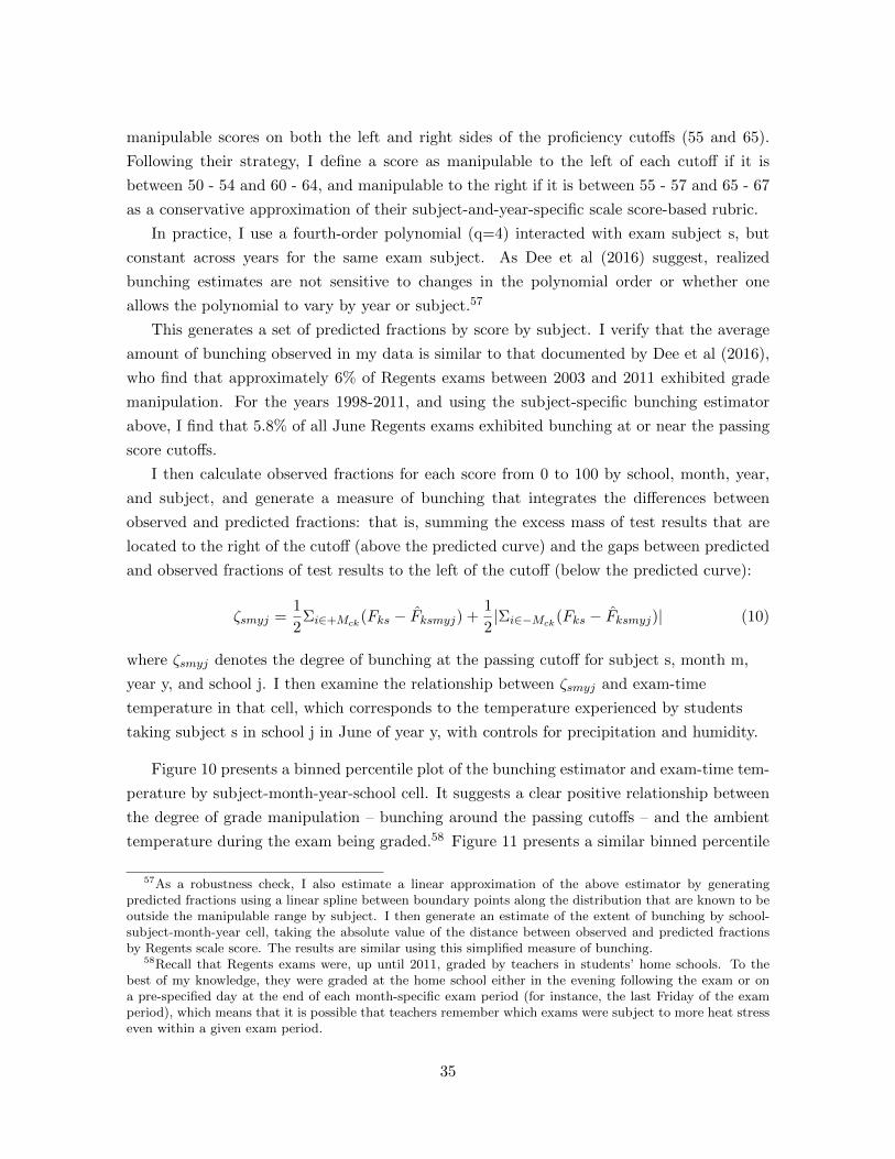
manipulable scores on both the left and right sides of the proficiency cutoffs (55 and 65).

Following their strategy, I define a score as manipulable to the left of each cutoff if it is

between 50 - 54 and 60 - 64, and manipulable to the right if it is between 55 - 57 and 65 - 67

as a conservative approximation of their subject-and-year-specific scale score-based rubric.

In practice, I use a fourth-order polynomial (q=4) interacted with exam subject s, but

constant across years for the same exam subject. As Dee et al (2016) suggest, realized

bunching estimates are not sensitive to changes in the polynomial order or whether one

allows the polynomial to vary by year or subject.57

This generates a set of predicted fractions by score by subject. I verify that the average

amount of bunching observed in my data is similar to that documented by Dee et al (2016),

who find that approximately 6% of Regents exams between 2003 and 2011 exhibited grade

manipulation. For the years 1998-2011, and using the subject-specific bunching estimator

above, I find that 5.8% of all June Regents exams exhibited bunching at or near the passing

score cutoffs.

I then calculate observed fractions for each score from 0 to 100 by school, month, year,

and subject, and generate a measure of bunching that integrates the differences between

observed and predicted fractions: that is, summing the excess mass of test results that are

located to the right of the cutoff (above the predicted curve) and the gaps between predicted

and observed fractions of test results to the left of the cutoff (below the predicted curve):

ζsmyj =1

2Σi∈+Mck

(Fks − F̂ksmyj) +1

2|Σi∈−Mck

(Fks − F̂ksmyj)| (10)

where ζsmyj denotes the degree of bunching at the passing cutoff for subject s, month m,

year y, and school j. I then examine the relationship between ζsmyj and exam-time

temperature in that cell, which corresponds to the temperature experienced by students

taking subject s in school j in June of year y, with controls for precipitation and humidity.

Figure 10 presents a binned percentile plot of the bunching estimator and exam-time tem-

perature by subject-month-year-school cell. It suggests a clear positive relationship between

the degree of grade manipulation – bunching around the passing cutoffs – and the ambient

temperature during the exam being graded.58 Figure 11 presents a similar binned percentile

57As a robustness check, I also estimate a linear approximation of the above estimator by generatingpredicted fractions using a linear spline between boundary points along the distribution that are known to beoutside the manipulable range by subject. I then generate an estimate of the extent of bunching by school-subject-month-year cell, taking the absolute value of the distance between observed and predicted fractionsby Regents scale score. The results are similar using this simplified measure of bunching.

58Recall that Regents exams were, up until 2011, graded by teachers in students’ home schools. To thebest of my knowledge, they were graded at the home school either in the evening following the exam or ona pre-specified day at the end of each month-specific exam period (for instance, the last Friday of the examperiod), which means that it is possible that teachers remember which exams were subject to more heat stresseven within a given exam period.

35

plot, but adding school fixed effects to allow for arbitrary differences in the average amount of

grade manipulation across schools. The clear positive association between bunching estimate

and temperature remains.

To assess the magnitude of this relationship controlling for school-, subject-, and/or year-

level differences in the degree of manipulation that are unrelated to temperature, I run a

series of regressions with ζsmyj as the dependent variable:

ζsmyj = δ0 + δ1Tsmyj + δ2Xsmyj + χj + εsmyj (11)

ζsmyj = δ0 + δ1Tsmyj + δ2Xsmyj + χj + ηs + θy + εsmyj (12)

ζsmyj = δ0 + δ1Tsmyj + δ2Xsmyj + χj + ηs + δ3Y eary + δ4Y ear2y + δ5Y ear

3y + εsmyj (13)

where Tsmyj denotes temperature, Xsmyj denotes precipitation and humidity, χj , ηs, and θy

denote school, subject, and year fixed effects respectively, and Y eary...Y ear3y denotes a

cubic time trend in scores. The parameter of interest is δ1, which represents the increase in

grade manipulation due to exam-time temperature.59

According to the estimates presented in Table 11, the amount of bunching increases by

approximately 0.10-0.16 percentage points per degree F, or 1.7% to 2.8% per degree F hotter

exam-time temperature relative to a mean of 5.8 percentage points. While these results are

highly suggestive of adaptive grading, it is of course not possible to infer teachers’ intentions.

It could be the case that teachers have an intuitive sense of whether a particular student scored

below his or her “true ability”, irrespective of whether or not this was due to temperature

or other exam-time conditions, and that they respond by manipulating grades in the case of

students on the passing margin.

8 Discussion and Conclusion

This paper explores the impact of heat stress on exam performance and educational attain-

ment. Using administrative data from the largest public school district in the United States,

I find that hot temperatures exert a causal, statistically significant, and economically mean-

ingful impact on student outcomes, by reducing student performance on high-stakes exams

59It is theoretically possible that if 1) teachers engage in punitive grade manipulation which is affected bynegative affect, which has been shown to increase with high temperatures, and 2) temperature on the day ofthe exam is positively correlated with temperature during grading, then the above estimates are attenuateddue to this reverse effect of punitive grading by hot-tempered teachers.

36

as well as reducing the amount of learning achieved over the course of the school year. The

research design exploits quasi-random variation in local temperature to identify the causal

impact of hot days on short run exam performance and long run educational attainment. The

breadth and depth of the data set allows not only for credible causal estimation of the adverse

impacts of heat stress, but also an assessment of possible adaptive responses by students and

teachers, which may be especially important in thinking about the potential human capital

impacts of future climate change.

Taking a high school exit exam on a 90◦ F day results in a 4.5% (0.17 standard deviation)

reduction in exam performance relative to a more optimal 72◦F day controlling for student

specific unobservables, which amounts to roughly 1/4 of the Black-White test score gap.

Given existing institutional rigidities – namely, cardinal pass/fail thresholds and graduation

requirements that depend on exam scores in a formulaic way – these short-run impacts on

student performance can have non-trivial knock-on effects on student attainment, leading to

a 10.88% reduction in the probability of passing that particular subject exam, and, for the

average New York City student, a roughly 2% lower likelihood of that student graduating on

time. Over the period 1998 to 2011, upwards of 510,000 exams that otherwise would have

passed received failing grades, affecting at least 90,000 students, possibly many more.

I find evidence supportive of the notion that heat stress can disrupt learning and thus

reduce the rate of human capital accumulation, which could have important implications for

both climate and education policy. Cumulative heat exposure over the course of the preced-

ing school year, measured by the number of days during the school year where temperatures

exceed 80◦F, is associated with significant reductions in end of year exam performance, con-

trolling for the exam-day effects of heat stress noted above. A year with five additional 80◦F+

days is associated with a 2.1% (-0.11 standard deviation) reduction in learning on average,

as measured by the same end of year regents exams, suggesting that heat exposure during

class time can reduce long-run human capital and educational attainment. These effects are

on par in magnitude with wiping out the gains from having a one standard deviation higher

value-added teacher for that school year, though more careful research is needed to examine

whether they result in comparable effects on later-life outcomes.

Using building level air-conditioning installation data, I find that air conditioning may

have a mild but incomplete protective effect, depending on how it is installed and utilized.

Building on evidence of grade manipulation by NYC teachers presented by Dee et al (2016),

I find that the extent of bunching at passing score cutoffs (evidence of grade manipulation)

is highly correlated with exam time temperature at the school and during the test session in

which any particular set of subject exams were administered, suggesting that teachers may

have been engaging in a form of “adaptive grading” to offset some of the adverse welfare

consequences of momentary heat stress during a high stakes exam, which presumably affects

students scores but does not reduce human capital per se.

37

These results have several implications. First, they imply that heat stress should be in-

cluded among the long list of inputs to the human capital production function that economists

have studied to date. This is especially true in light of the fact that climate change will lead

to greater additional heat exposure for poorer populations both across and within countries

given well documented relationships between income and hot current climate (Acemoglu and

Dell, 2010; Park et al, 2015) as well as between income and air conditioning ownership (Davis

and Gertler, 2015).

From the perspective of climate policy, this study lends further support to the notion

that direct human impacts of heat stress should be included in climate damage functions

and resulting social cost of carbon estimates (Tol, 2009; Burke et al, 2016; Heal and Park,

2016). They suggest that climate change may act to reduce not only the level of output but

the growth rate as well, if added heat stress reduces the rate of human capital accumula-

tion. These results also seem to underscore the importance of taking the interaction between

weather shocks and existing institutions into account in assessing the realized welfare impacts

of climate change.60

From a methodological perspective, these findings support the use of weather instruments

as a means of isolating truly random variation in test scores, which can in principle be used

to inform the issue of score fade out (Cascio and Staiger, 2012; Chetty et al, 2010).

In terms of our understanding of the role of climate in economic development, this study

lends further evidence that the longstanding correlation between geography and economic

growth (Gallup, Sachs, Mellinger, 1999; Acemoglu, Johnson, and Robinson, 2000; Rodrik et

al, 2004) may have a causal as opposed to merely correlational component.

The findings from this study suggest several fruitful avenues for future research, and raises

a number of policy-relevant questions. If heat exposure can affect both short- and long-run

student performance, how much of the residual racial (Black-White, Hispanic-White) test-

score gap be a function of climatic factors?61 If heat stress during high stakes standardized

testing affects exam performance differentially across regions, could standardized exams such

as the SAT or GRE that are curved relative to a national population exhibit general equi-

librium impacts? Finally, do the effects documented here generalize to developing country

contexts such as India or Sub-Saharan Africa, where present and future heat burdens are

likely to be more severe?

60Such institutional factors may be especially important in thinking about the welfare consequences of heatin the human capital production process if they exacerbate underlying principal-agent problems. For instance,school principals may not fully internalize the welfare costs of elevated school temperatures (lack of propercooling equipment) if the link between principal behavior and student outcomes is imperfectly observable.The result may be a socially inefficient investment in this particular form of productive capital.

61Blacks and Hispanics are more likely to reside in hotter states and to attend school in highly urbanizeddistricts, which may be subject to additional urban heat island effects.

38

References

1. Acemoglu, Daron, Simon Johnson, and James A. Robinson. The colonial origins of comparative

development: An empirical investigation. No. w7771. National bureau of economic research,

2000.

2. Acemoglu, Daron, and Melissa Dell. ”Productivity differences between and within countries.”

American Economic Journal: Macroeconomics 2.1 (2010): 169-188.

3. Aizer, Anna, Janet Currie, Peter Simon, and Patrick Vivier. ”Lead Exposure and Racial

Disparities in Test Scores.” Brown Univ. Work. Pap (2015).

4. Alexander, Karl L., Doris R. Entwisle, and Linda S. Olson. ”Schools, achievement, and in-

equality: A seasonal perspective.” Educational Evaluation and Policy Analysis 23.2 (2001):

171-191.

5. Albouy, David, et al. Climate amenities, climate change, and American quality of life. No.

w18925. National Bureau of Economic Research, 2013.

6. Allcott, Hunt, and Michael Greenstone. ”Is there an energy efficiency gap?.” The Journal of

Economic Perspectives 26.1 (2012): 3-28.

7. Angrist, Joshua D., and Victor Lavy. ”Using Maimonides’ Rule to Estimate the Effect of Class

Size on Scholastic Achievement.” The Quarterly Journal of Economics 114.2 (1999): 533-575.

8. Anthoff, David, Cameron Hepburn, and Richard SJ Tol. ”Equity weighting and the marginal

damage costs of climate change.” Ecological Economics 68.3 (2009): 836-849.

9. Anderson, Craig A. ”Temperature and aggression: effects on quarterly, yearly, and city rates of

violent and nonviolent crime.” Journal of personality and social psychology 52.6 (1987): 1161.

10. Anderson, Craig A., and Dona C. Anderson. ”Ambient temperature and violent crime: Tests of

the linear and curvilinear hypotheses.” Journal of personality and social psychology 46.1 (1984):

91.

11. Becker, Gary S. ”Investment in human capital: A theoretical analysis.” The journal of political

economy (1962): 9-49.

12. Billings, Stephen B., David J. Deming, and Jonah Rockoff. ”School Segregation, Educational

Attainment, and Crime: Evidence from the End of Busing in Charlotte-Mecklenburg.” The

Quarterly journal of economics 129.1 (2014): 435-476.

13. Bowler, K., and R. Tirri. The temperature characteristics of synaptic membrane ATPases from

immature and adult rat brain. Journal of neurochemistry 23, no. 3 (1974): 611-613.

14. Burke, Marshall, and Kyle Emerick. ”Adaptation to Climate Change: Evidence from US

Agriculture.” (2015).

39

15. Burke, Marshall, Solomon M. Hsiang, and Edward Miguel. ”Global non-linear effect of temper-

ature on economic production.” Nature (2015).

16. Burke M, Craxton M, Kolstad CD, Onda C, Allcott H, Baker E, Barrage L, Carson R, Gilling-

ham K, Graff-Zivin J, Greenstone M. Opportunities for advances in climate change economics.

Science. 2016 Apr 15;352(6283):292-3.

17. Cachon, Gerard, Santiago Gallino, and Marcelo Olivares. ”Severe weather and automobile

assembly productivity.” Columbia Business School Research Paper 12/37 (2012).

18. Cascio, Elizabeth U., and Douglas O. Staiger. Knowledge, tests, and fadeout in educational

interventions. No. w18038. National Bureau of Economic Research, 2012.

19. Card, David, and Jesse Rothstein. ”Racial segregation and the black?white test score gap.”

Journal of Public Economics 91.11 (2007): 2158-2184.

20. Chay, Kenneth Y., and Michael Greenstone. ”Does Air Quality Matter? Evidence from the

Housing Market.” Journal of Political Economy 113.2 (2005).

21. Chetty, R., Friedman, J. N., Hilger, N., Saez, E., Schanzenbach, D. W., and Yagan, D. (2010).

How does your kindergarten classroom affect your earnings? Evidence from Project STAR (No.

w16381). National Bureau of Economic Research.

22. Chetty, Raj, John N. Friedman, and Jonah E. Rockoff. ”Measuring the Impacts of Teachers I:

Evaluating Bias in Teacher Value-Added Estimates.” THE AMERICAN ECONOMIC REVIEW

104.9 (2014): 2593-2632.

23. Chetty, Raj, John N. Friedman, and Jonah E. Rockoff. ”Measuring the Impacts of Teachers II:

Teacher Value-Added and Student Outcomes in Adulthood.” THE AMERICAN ECONOMIC

REVIEW 104.9 (2014): 2633-2679.

24. Chetty, Raj, Nathaniel Hendren, and Lawrence F. Katz. The effects of exposure to better

neighborhoods on children: New evidence from the Moving to Opportunity experiment. No.

w21156. National Bureau of Economic Research, 2015.

25. Cragg, Michael I., and Matthew E. Kahn. ”Climate consumption and climate pricing from 1940

to 1990.” Regional Science and Urban Economics 29.4 (1999): 519-539.

26. Currie, J., Hanushek, E. A., Kahn, E. M., Neidell, M., & Rivkin, S. G. (2009). Does pollution

increase school absences?. The Review of Economics and Statistics, 91(4), 682-694.

27. Currie, Janet. ”Healthy, Wealthy, and Wise: Socioeconomic Status, Poor Health in Childhood,

and Human Capital Development.” Journal of Economic Literature (2009): 87-122.

28. Davis, Lucas W., and Paul J. Gertler. ”Contribution of air conditioning adoption to future

energy use under global warming.” Proceedings of the National Academy of Sciences 112.19

(2015): 5962-5967.

40

29. Dell, Melissa, Benjamin F. Jones, and Benjamin A. Olken. ”Temperature shocks and economic

growth: Evidence from the last half century.” American Economic Journal: Macroeconomics

4.3 (2012): 66-95.

30. Dell, Melissa, Benjamin F. Jones, and Benjamin A. Olken. ”What do we learn from the weather?

The new climateeconomy literature.” Journal of Economic Literature 52.3 (2014): 740-798.

31. Deming, David J., Justine S. Hastings, Thomas J. Kane, and Douglas O. Staiger. ”School

choice, school quality, and postsecondary attainment.” The American economic review 104, no.

3 (2014): 991-1013.

32. Deryugina, Tatyana, and Solomon M. Hsiang. ”Does the environment still matter? Daily

temperature and income in the United States.” (2014).

33. Deschnes, Olivier and Michael Greenstone. 2011. ”Climate Change, Mortality, and Adapta-

tion: Evidence from Annual Fluctuations in Weather in the US.” American Economic Journal:

Applied Economics, 3(4): 152-85.

34. Deschenes, Olivier, and Enrico Moretti. ”Extreme weather events, mortality, and migration.”

The Review of Economics and Statistics 91.4 (2009): 659-681.

35. Diamond, Rebecca, and Petra Persson. The Long-term Consequences of Teacher Discretion in

Grading of High-stakes Tests. No. w22207. National Bureau of Economic Research, 2016.

36. Duran-Narucki, Valkiria. ”School building condition, school attendance, and academic achieve-

ment in New York City public schools: A mediation model.” Journal of environmental psychol-

ogy 28.3 (2008): 278-286.

37. Energy Information Administration, 2009. Residential Energy Consumption Survey.

38. Fitzpatrick, C., McKinnon, R. D., Blair, C. B., & Willoughby, M. T. (2014). Do preschool

executive function skills explain the school readiness gap between advantaged and disadvantaged

children?. Learning and Instruction, 30, 25-31.

39. Fogel, R. W. (2004). Health, Nutrition, and Economic Growth*. Economic Development and

Cultural Change, 52(3), 643-658.

40. Gaffin, S. R., Rosenzweig, C., Khanbilvardi, R., Parshall, L., Mahani, S., Glickman, H., . . .

& Hillel, D. (2008). Variations in New York City’s urban heat island strength over time and

space. Theoretical and applied climatology, 94(1-2), 1-11.

41. Gallup, John Luke, Jeffrey D. Sachs, and Andrew D. Mellinger. ”Geography and economic

development.” International regional science review 22.2 (1999): 179-232.

42. Glewwe, Paul, and Michael Kremer. ”Schools, teachers, and education outcomes in developing

countries.” Handbook of the Economics of Education 2 (2006): 945-1017.

43. Goldin, Claudia Dale, and Lawrence F. Katz. The race between education and technology.

Harvard University Press, 2009.

41

44. Goodman, Joshua. Flaking out: Student absences and snow days as disruptions of instructional

time. No. w20221. National Bureau of Economic Research, 2014.

45. Goodman, Joshua, and Jisung Park. Hot Takes: Temperature, Student Performance, and the

Racial Achievement Gap. Unpublished Manuscript. 2016

46. Greenstone, Michael, Elizabeth Kopits, and Ann Wolverton. ”Developing a social cost of car-

bon for US regulatory analysis: A methodology and interpretation.” Review of Environmental

Economics and Policy 7, no. 1 (2013): 23-46.

47. Greenstone, Michael, and B. Kelsey Jack. ”Envirodevonomics: A research agenda for an emerg-

ing field.” Journal of Economic Literature 53.1 (2015): 5-42.

48. Grether, W. (1973). ”Human performance at elevated environmental temperatures.” Aerospace

Medicine 44(7): 747-755.

49. Greenstone, Michael, Elizabeth Kopits, and Ann Wolverton. ”Developing a social cost of car-

bon for US regulatory analysis: A methodology and interpretation.” Review of Environmental

Economics and Policy 7.1 (2013): 23-46.

50. Hallegatte, Stephane. “Strategies to adapt to an uncertain climate change.” Global Environ-

mental Change 19.2 (2009): 240-247.

51. Hanushek, Eric A., and Ludger Woessmann. ”Do better schools lead to more growth? Cognitive

skills, economic outcomes, and causation.” Journal of Economic Growth 17.4 (2012): 267-321.

52. Hocking, Chris, Richard B. Silberstein, Wai Man Lau, Con Stough, and Warren Roberts. “Eval-

uation of cognitive performance in the heat by functional brain imaging and psychometric test-

ing. Comparative Biochemistry and Physiology Part A: Molecular Integrative Physiology 128,

no. 4 (2001): 719-734.

53. Hogrefe, C., Biswas, J., Lynn, B., Civerolo, K., Ku, J. Y., Rosenthal, J., & Kinney, P. L. (2004).

Simulating regional-scale ozone climatology over the eastern United States: model evaluation

results. Atmospheric Environment, 38(17), 2627-2638.

54. Hsiang, Solomon M. ”Temperatures and cyclones strongly associated with economic production

in the Caribbean and Central America.” Proceedings of the National Academy of sciences 107.35

(2010): 15367-15372.

55. Hsiang, Solomon M., Marshall Burke, and Edward Miguel. ”Quantifying the influence of climate

on human conflict.” Science 341.6151 (2013): 1235367.

56. Isen, A., Rossin-Slater, M., & Walker, R. (2015). Heat and long-run human capital formation.

Unpublished Manuscript.

57. Jaffe, Adam B., and Robert N. Stavins. ”The energy-efficiency gap What does it mean?.”

Energy policy 22.10 (1994): 804-810.

42

58. Kahn, M. The Climate Change Adaptation Literature. Rev Environ Econ Policy 2016.

59. Kenrick, Douglas T., and Steven W. MacFarlane. ”Ambient temperature and horn honking a

field study of the heat/aggression relationship.” Environment and behavior 18.2 (1986): 179-

191.

60. Krueger, Alan B., and Diane M. Whitmore. ”The effect of attending a small class in the early

grades on collegetest taking and middle school test results: Evidence from Project STAR.” The

Economic Journal 111.468 (2001): 1-28.

61. Lavy, Victor, Avraham Ebenstein, and Sefi Roth. The impact of short term exposure to ambient

air pollution on cognitive performance and human capital formation. No. w20648. National

Bureau of Economic Research, 2014.

62. Lavy, Victor, Avraham Ebenstein, and Sefi Roth. The Long Run Human Capital and Eco-

nomic Consequences of High-Stakes Examinations. No. w20647. National Bureau of Economic

Research, 2014.

63. Lavy, Victor. ”Performance Pay and Teachers’ Effort, Productivity, and Grading Ethics.” The

American economic review 99.5 (2009): 1979-2011.

64. Lavy, Victor. Long run effects of free school choice: College attainment, employment, earnings,

and social outcomes at adulthood. No. w20843. National Bureau of Economic Research, 2015.

65. Mackworth, Norman H. ”Effects of heat on wireless operators.” British journal of industrial

medicine 3.3 (1946): 143.

66. Maddala, Gangadharrao Soundaryarao, and Kajal Lahiri. Introduction to econometrics. Vol.

2. New York: Macmillan, 1992.

67. Mankiw, N. Gregory, David Romer, and David N. Weil. ”A Contribution to the Empirics of

Economic Growth.” The Quarterly Journal of Economics 107.2 (1992): 407-437.

68. Mansur, Erin T., Robert Mendelsohn, and Wendy Morrison. ”Climate change adaptation:

A study of fuel choice and consumption in the US energy sector.” Journal of Environmental

Economics and Management 55.2 (2008): 175-193.

69. Melillo, Jerry M., Terese TC Richmond, and G. W. Yohe. ”Climate change impacts in the

United States.” Third National Climate Assessment (2014).

70. Mendell, Mark J., and Garvin A. Heath. ”Do indoor pollutants and thermal conditions in

schools influence student performance? A critical review of the literature.” Indoor air 15.1

(2005): 27-52.

71. Mincer, Jacob. ”Investment in human capital and personal income distribution.” The journal

of political economy (1958): 281-302.

72. Niu, Jianlei. ”Some significant environmental issues in high-rise residential building design in

urban areas.” Energy and buildings 36.12 (2004): 1259-1263.

43

73. Park, Jisung. Will We Adapt? Temperature Shocks, Labor Productivity and Climate Adapta-

tion in the United States. Harvard Project on Climate Agreements Working Papers, 2015

74. Raichle, Marcus E., and Mark A. Mintun. Brain work and brain imaging. Annual Review of

Neuroscience 29 (2006): 449-476.

75. Roback, J (1982) Wages, Rents, and the Quality of Life Journal of Political Economy Vol. 90

No. 6 pp1257-1278.

76. Rodrik, Dani, Arvind Subramanian, and Francesco Trebbi. ”Institutions rule: the primacy

of institutions over geography and integration in economic development.” Journal of economic

growth 9.2 (2004): 131-165.

77. Rosen, S. (1974) Hedonic Prices and Implicit Markets: Product Differentiation in Pure Com-

petition Journal of Political Economy 82: 34-55.

78. Rosenzweig, Cynthia, William Solecki, and Ronald Slosberg. ”Mitigating New York Citys heat

island with urban forestry, living roofs, and light surfaces.” A report to the New York State

Energy Research and Development Authority (2006).

79. Sandstrm, F. Mikael, and Fredrik Bergstrm. ”School vouchers in practice: Competition will

not hurt you.” Journal of Public economics 89.2 (2005): 351-380.

80. Schoer, L. and Shaffran, J. (1973) A combined evaluation of three separate research projects on

the effects of thermal environment on learning and performance, ASHRAE Trans., 79, 97108.

81. Schultz, Theodore W. ”Investment in human capital.” The American economic review (1961):

1-17.

82. Schiff, Steven J., and George G. Somjen.The effects of temperature on synaptic transmission in

hippocampal tissue slices. Brain Research 345, no. 2 (1985): 279-284.

83. Seppanen, Olli, William J. Fisk, and Q. H. Lei. ”Effect of temperature on task performance in

office environment.” Lawrence Berkeley National Laboratory (2006).

84. Sievertsen, Hans Henrik, Francesca Gino, and Marco Piovesan. ”Cognitive fatigue influences

students’ performance on standardized tests.” Proceedings of the National Academy of Sciences

(2016): 201516947.

85. Sinha, Paramita, and Maureen L. Cropper. Household Location Decisions and the Value of

Climate Amenities. No. w21826. National Bureau of Economic Research, 2015.

86. Stock, James H., and Mark W. Watson. ”Introduction to econometrics.” (2007).

87. Sudarshan, Anant, and Meenu Tewari. The economic impacts of temperature on industrial

productivity: Evidence from indian manufacturing. Working Paper, 2013.

88. Vasmatzidis, Ioannis, Robert E. Schlegel, and Peter A. Hancock. An investigation of heat stress

effects on time-sharing performance. Ergonomics 45, no. 3 (2002): 218-239.

44

89. Weil, David N. ”Accounting for the Effect of Health on Economic Growth.” The Quarterly

Journal of Economics (2007): 1265-1306.

90. Zafar, Basit. ’How Do College Students Form Expectations?’. Journal of Labor Economics 29.2

(2011): 301?348

91. Zivin, Joshua Graff, and Matthew Neidell. ”The Impact of Pollution on Worker Productivity.”

The American Economic Review 102.7 (2012): 3652-3673.

92. Zivin, Joshua Graff, and Matthew Neidell. ”Temperature and the allocation of time: Implica-

tions for climate change.” Journal of Labor Economics 32.1 (2014): 1-26.

93. Zivin, Joshua S. Graff, Solomon M. Hsiang, and Matthew J. Neidell. Temperature and Human

Capital in the Short-and Long-run. No. w21157. National Bureau of Economic Research, 2015.

94. Zivin, Joshua Graff, and Jeffrey Shrader. ”Temperature Extremes, Health, and Human Capi-

tal.” The Future of Children (2016): 31-50.

45

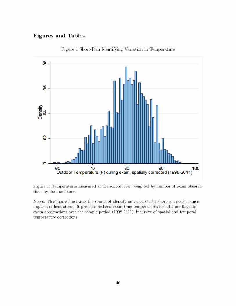
Figures and Tables

Figure 1 Short-Run Identifying Variation in Temperature

Figure 1: Temperatures measured at the school level, weighted by number of exam observa-tions by date and time

Notes: This figure illustrates the source of identifying variation for short-run performanceimpacts of heat stress. It presents realized exam-time temperatures for all June Regentsexam observations over the sample period (1998-2011), inclusive of spatial and temporaltemperature corrections.

46

Figure 2 Short-Run Identifying Variation in Temperature

Figure 2: Temperatures measured at the school level, weighted by student population.

Notes: This figure illustrates the source of identifying variation for short-run performanceimpacts of heat stress. It presents realized exam-time temperatures for two subsequent dayswithin a Regents exam period – Thursday, June 24th, 2010, and Friday, June 25th, 2010 –inclusive of spatial and temporal temperature corrections described in section 4, plottingobservations at the student-exam level.

47

Figure 3 Variation in Cumulative Heat Exposure by Borough and Year in New YorkCity

Figure 3: Temperatures measured at the nearest weather station (borough) level.

Notes: This figure illustrates year to year variation in cumulative heat exposure during theschool year, measured in terms of the number of days with max temperatures above 80◦Fper school year. Temperature readings are taken from USGS weather stations, one fromeach of the five boroughs of NYC.

48

Figure 4 Air Conditioning Status by NYC Public School Building

Figure 4: NYC Public School Buildings by AC status

Notes: This figure provides a map of New York City public schools, with green dotsrepresenting schools that had any air conditioning equipment as of 2012, and red dotsrepresenting schools that did not, according to the NY School Construction Authority.

49

Table 1: Summary Statistics by Borough

Borough Regents Score Pass Rate Proficiency Rate Previous Ability

Bronx 60.86 0.48 0.23 -0.19(18.17) (0.50) (0.42) (1.40)

Brooklyn 64.96 0.58 0.32 0.17(17.81) (0.49) (0.47) (1.41)

Manhattan 66.66 0.61 0.36 0.31(18.08) (0.49) (0.48) (1.49)

Queens 65.81 0.60 0.34 0.23(17.42) (0.49) (0.47) (1.33)

Staten Island 67.38 0.63 0.37 0.43(17.23) (0.48) (0.48) (1.44)

Total 64.86 0.57 0.32 0.16(17.92) (0.49) (0.47) (1.42)

Notes: Previous ability denotes a combined z-score for standardized English Language andArts (ELA) and math exams taken in 3rd-8th grade for the students in the Regents examsample.

Table 2: Summary Statistics by Ethnicity

Ethnicity Regents Score Pass Rate Proficiency Rate Previous Ability

Asian 74.73 0.78 0.57 0.98(16.80) (0.41) (0.49) (1.54)

Black 61.21 0.50 0.23 -0.18(17.05) (0.50) (0.42) (1.34)

Hispanic 61.49 0.51 0.24 -0.16(17.23) (0.50) (0.42) (1.32)

Multiracial 69.65 0.69 0.44 0.34(17.44) (0.46) (0.50) (1.26)

Native American 61.96 0.51 0.26 -0.22(18.08) (0.50) (0.44) (1.45)

White 72.92 0.75 0.52 1.02(16.78) (0.43) (0.50) (1.56)

Total 64.86 0.57 0.32 0.16(17.92) (0.49) (0.47) (1.42)

Notes: This figure presents summary statistics for key outcome variables by demographicsub-group. Missing observations correspond to the 14% of students for whom Regentsscores and scrambled student id’s are available but demographic information is not.

50

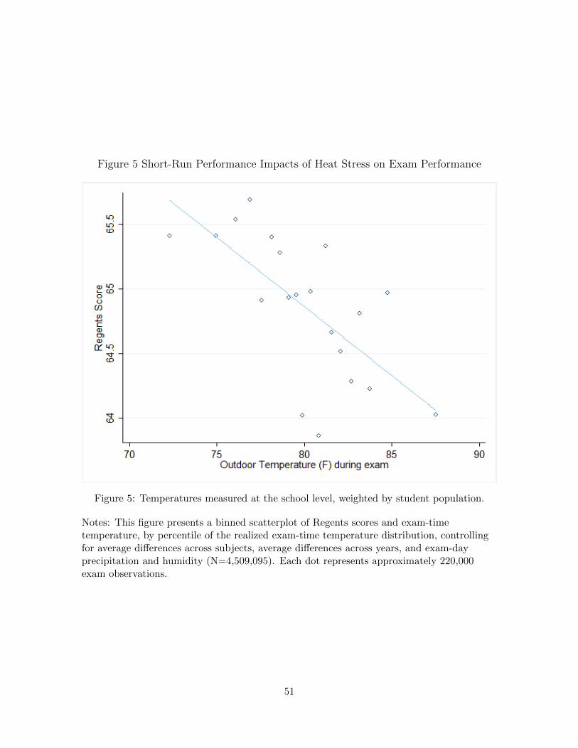
Figure 5 Short-Run Performance Impacts of Heat Stress on Exam Performance

Figure 5: Temperatures measured at the school level, weighted by student population.

Notes: This figure presents a binned scatterplot of Regents scores and exam-timetemperature, by percentile of the realized exam-time temperature distribution, controllingfor average differences across subjects, average differences across years, and exam-dayprecipitation and humidity (N=4,509,095). Each dot represents approximately 220,000exam observations.

51

Table 3 Short-Run Performance Impacts of Heat Stress on Exam Performance:Regents Scores for NYC Public High School Students

(1) (2) (3)Score Score Score

Temperature (◦F) -0.138∗∗∗ -0.131∗∗∗ -0.109∗∗

(0.0353) (0.0335) (0.0365)

Precipitation (10mm) 0.0413∗ 0.0397∗ 0.0447∗

(0.0174) (0.0175) (0.0190)

Afternoon -0.526∗ -0.728∗∗

(0.223) (0.254)

Day of week 0.434∗∗∗

(0.0861)

Day of month -0.116(0.0678)

Fixed Effects

Student X X XYear X X XSubject X X X

N 4347719 4347719 4347719r2 0.709 0.709 0.709

Standard errors in parentheses∗ p < 0.05, ∗∗ p < 0.01, ∗∗∗ p < 0.001

Table 3: Dependent variable is Regents scoreNotes: Observations are at student-exam-date-time-level. Student, subject, and year fixedeffects suppressed in output, and 161,383 singleton observations are dropped. June Regentsexams in 11 core subjects only, for years 1998-2011. All regressions include controls fordewpoint. Temperature is temporally corrected to account for diurnal fluctuations (AM vsPM sessions, see Appendix), and spatially corrected to account for urban heat island effects(see Appendix). Robust standard errors are clustered at borough by date and time level.

52

Table 4 Short-Run Performance Impacts of Heat Stress on Exam Performance:Regents Exam Pass Rates for NYC Public High School Students

(1) (2) (3)Pass Pass Pass

Temperature -0.00311∗∗∗ -0.00294∗∗∗ -0.00225∗∗

(0.000778) (0.000740) (0.000769)

Precipitation (mm) 0.000886∗ 0.000845∗ 0.00105∗

(0.000413) (0.000414) (0.000452)

Afternoon -0.0128∗ -0.0189∗∗

(0.00527) (0.00607)

Day of week 0.00831∗∗∗

(0.00212)

Day of month -0.00332∗

(0.00164)

Fixed Effects

Student X X XYear X X XSubject X X X

N 4347719 4347719 4347719r2 0.550 0.550 0.551

Standard errors in parentheses∗ p < 0.05, ∗∗ p < 0.01, ∗∗∗ p < 0.001

Table 4: Dependent variable is Dummy for Passed Regents examNotes: Observations are at student-exam-date-time-level. Student, subject, and year fixedeffects suppressed in output, and 161,383 singleton observations are dropped. All regressionsinclude controls for dewpoint. June Regents exams in 11 core subjects only, for years1998-2011. Temperature is temporally corrected to account for diurnal fluctuations (AM vsPM sessions, see Appendix), and spatially corrected to account for urban heat island effects(see Appendix). Robust standard errors are clustered at borough by date and time level.

53

Table 5 Short-Run Performance Impacts of Heat Stress on Exam Performance:Regents Exam Proficiency Status for NYC Public High School Students

(1) (2) (3)Proficient Proficient Proficient

Temperature (F) -0.00309∗∗∗ -0.00296∗∗∗ -0.00242∗∗

(0.000693) (0.000673) (0.000795)

Precipitation (10mm) 0.00128∗∗∗ 0.00125∗∗∗ 0.00139∗∗∗

(0.000337) (0.000336) (0.000339)

Afternoon -0.00964∗ -0.0144∗∗

(0.00443) (0.00533)

Day of week 0.00849∗∗∗

(0.00195)

Day of month -0.00270∗

(0.00133)

Fixed Effects

Student X X XYear X X XSubject X X X

N 4347719 4347719 4347719r2 0.611 0.612 0.612

Standard errors in parentheses∗ p < 0.05, ∗∗ p < 0.01, ∗∗∗ p < 0.001

Table 5: Dependent variable is dummy for Proficiency status achievedNotes: Observations are at student-exam-date-time-level. Student, subject, and year fixedeffects suppressed in output, and 161,383 singleton observations are dropped. June Regentsexams in 11 core subjects only, for years 1998-2011. All regressions include controls fordewpoint. Temperature is temporally corrected to account for diurnal fluctuations (AM vsPM sessions, see Appendix), and spatially corrected to account for urban heat island effects(see Appendix). Robust standard errors are clustered at borough by date and time level.

54

Figure 6 Previous Standardized Exam Scores and Regents Performance

Figure 6: Combined ELA/math z-scores as a measure of student ability.

Notes: This figure presents a binned scatterplot of Regents scores and previous z-scores(ELA and math z-scores by grade and year, averaged by student) by percentile of thecombined z-score distribution.

55

Tab

le6

Het

erog

enei

tyin

Shor

t-R

un

Impac

tsby

Dem

ogra

phic

Sub-G

roup

All

Asi

anB

lack

His

pan

icW

hit

eM

ale

Fem

ale

FS

SL

un

ch

(1)

(2)

(3)

(4)

(5)

(6)

(7)

(8)

Sco

reS

core

Sco

reS

core

Sco

reS

core

Sco

reS

core

Tem

per

atu

re(F

)-0

.109∗∗

-0.0

538∗

-0.0

701

-0.0

674∗

-0.0

658∗

-0.0

618∗

-0.0

761∗

-0.0

669∗

(0.0

365)

(0.0

254)

(0.0

386)

(0.0

338)

(0.0

318)

(0.0

292

)(0

.0310

)(0

.0301

)

Pre

cip

itati

on

(10m

m)

0.04

47∗

0.03

45∗

0.05

28∗

0.06

05∗∗

0.03

380.

042

7∗0.0

547∗∗

0.048

3∗∗

(0.0

190)

(0.0

156)

(0.0

219)

(0.0

207)

(0.0

188)

(0.0

184

)(0

.0176

)(0

.0179

)

Day

ofw

eek

0.43

4∗∗∗

0.04

000.

427∗∗∗

0.33

0∗∗∗

0.15

70.

309∗∗∗

0.263∗∗

0.309∗∗∗

(0.0

861)

(0.0

831)

(0.0

938)

(0.0

887)

(0.0

946)

(0.0

837

)(0

.0813

)(0

.0814

)

Day

ofm

onth

-0.1

16-0

.002

95-0

.087

6-0

.126

-0.1

41∗

-0.0

635

-0.1

20∗

-0.0

901

(0.0

678

)(0

.061

1)(0

.073

5)(0

.070

8)(0

.067

2)(0

.063

0)(0

.060

6)(0

.060

8)

Aft

ern

oon

-0.7

28∗∗

-0.2

09-0

.928∗∗∗

-0.9

07∗∗∗

-0.5

99∗

-0.7

32∗∗

-0.7

96∗∗∗

-0.8

13∗∗∗

(0.2

54)

(0.2

44)

(0.2

74)

(0.2

64)

(0.2

70)

(0.2

35)

(0.2

32)

(0.2

28)

N4347

719

6214

6013

3224

514

3134

254

6286

2075

490

189

0026

363

3600

r20.

709

0.73

40.

661

0.65

50.

752

0.712

0.709

0.6

98

Sta

ndard

erro

rsin

pare

nth

eses

∗p<

0.0

5,∗∗p<

0.0

1,∗∗∗p<

0.0

01

Tab

le6:

Dep

end

ent

vari

able

isR

egen

tssc

ore

Note

s:O

bse

rvat

ion

sar

eat

stu

den

t-ex

am-d

ate-

tim

e-le

vel.

Stu

den

t,su

bje

ct,

and

year

fixed

effec

tssu

pp

ress

edin

ou

tpu

t.Ju

ne

Reg

ents

exam

sin

11co

resu

bje

cts

on

ly,

for

year

s19

98-2

011.

All

regr

essi

ons

incl

ud

eco

ntr

ols

for

dew

poin

t.T

emp

eratu

reis

tem

pora

lly

corr

ecte

dto

acco

unt

for

diu

rnal

flu

ctu

atio

ns

(AM

vs

PM

sess

ion

s,se

eA

pp

end

ix),

and

spat

iall

yco

rrec

ted

toac

cou

nt

for

urb

an

hea

tis

lan

deff

ects

(see

Ap

pen

dix

).R

obu

stst

and

ard

erro

rsar

ecl

ust

ered

atb

orou

ghby

date

an

dti

me

leve

l.

56

Figure 7 4-year Graduation Status and Average Exam-Time Outdoor Temperatureby student for NYC Public High School Students

Figure 7: Dependent Variable is Dummy for Graduated in 4 Years

Notes: This figure presents a binned scatterplot of 4-year graduation status by percentile ofthe observed average exam-time temperature distribution, where exam-time temperaturefor all June Regents core subject exam sessions during the first three years of high schoolare averaged by student, plotting residual variation after controls for the total number ofexams taken by student as well as student-level observables (ethnicity, gender, averageprevious z-scores, federally subsidized school lunch eligibility) and average precipitation atthe school level are included.

57

Table 7: Knock-on Impacts, 4 Year Graduation Rates

(1) (2) (3)Graduated (4yrs) Graduated (4yrs) Graduated (4yrs)

Mean Temperature (F) -0.00132∗∗ -0.00146∗∗∗ -0.00172∗∗∗

(0.000414) (0.000378) (0.000413)

Mean Precipitation (10mm) 0.00106∗ 0.00596∗∗∗ 0.00367∗∗∗

(0.000509) (0.000512) (0.000369)

Previous Ability 0.0946∗∗∗ 0.0903∗∗∗ 0.0833∗∗∗

(0.000740) (0.000719) (0.000689)

Fixed Effects

Number of Takes X X XCohort X XSchool X

N 398736 398736 398692r2 0.238 0.262 0.319

Standard errors in parentheses∗ p < 0.05, ∗∗ p < 0.01, ∗∗∗ p < 0.001

Notes: Observations are at the student level. Robust standard errors are clustered atborough by date and time level. All regressions include controls for daily precipitation anddewpoint. Number of takes, cohort, and school fixed effects are suppressed in output.Temperature is temporally corrected to account for diurnal fluctuations, and spatiallycorrected to account for urban heat island effects. Average temperatures from all JuneRegents exam takes during the students’ first four years of high school are computed bystudent.

58

Table 8: Knock-on Impacts, 4, 5, 6 Year Graduation Rates

(1) (2) (3) (4)Grad (4yrs) Grad (5yrs) Grad (6yrs) Evergrad

Mean Temperature (F) -0.00172∗∗∗ -0.00224∗∗∗ -0.00179∗∗∗ -0.00161∗∗∗

(0.000413) (0.000414) (0.000411) (0.000408)

Mean Precipitation (10mm) 0.00367∗∗∗ 0.00287∗∗∗ 0.00254∗∗∗ 0.00254∗∗∗

(0.000369) (0.000353) (0.000340) (0.000341)

Previous Ability 0.0833∗∗∗ 0.0745∗∗∗ 0.0685∗∗∗ 0.0693∗∗∗

(0.000689) (0.000653) (0.000627) (0.000626)

N 398692 386663 394911 398692r2 0.319 0.374 0.388 0.383

Standard errors in parentheses∗ p < 0.05, ∗∗ p < 0.01, ∗∗∗ p < 0.001

Notes: Observations at the student level for those students for whom all outcomes areavailable in dataset. Robust standard errors are clustered at school by date and time level.All regressions include controls for daily precipitation and dewpoint. Number of takes,cohort, and school fixed effects are suppressed in output. Temperature is temporallycorrected to account for diurnal fluctuations (AM vs PM sessions, see Appendix), andspatially corrected to account for urban heat island effects (see Appendix). Averagetemperatures from all June Regents exam takes during the students’ first four years of highschool are computed by student.

59

Figure 8: Cumulative Learning Impacts of Heat Exposure during the PrecedingSchool Year (Regents Exam Scores for NYC Public High School Students)

Figure 8: Temperatures measured at the school level, weighted by student population.

Notes: This figure presents a binned scatterplot of end-of-year Regents performance at theschool-subject-date level, by quantile of the distribution of cumulative heat stress, measuredby the number of days per degree bin (showing days with maximum temperatures above80◦F), plotting residual variation after controls for exam-day temperature andprecipitation, as well as school-, subject-, time of day, day of week, and day of month fixedeffects are included.

60

Table 9: Cumulative Learning Impacts of Heat Exposure during School Year

(1)Score

(2)Score

(3)Score

(4)Score

Days with max temp 70F-80F -0.16525*** -0.059 -0.10129* -0.12900*0.042 0.062 0.058 0.073

Days with max temp80F-90F

-0.11675* -0.15285* -0.22916** -0.106

0.062 0.093 0.093 0.119Days with max tempabove 90F

0.214 -0.132 0.151 -0.018

0.172 0.220 0.180 0.319Days with max temp below 20F 0.117 0.899

0.454 0.635Days with max temp20F-30F

0.005 -0.055

0.095 0.105Days with max temp30F-40F

-0.10122*** -0.09219***

0.028 0.026Days with max temp40F-50F

0.002

0.076Days with max temp50F-60F

0.082

0.050Exam-Time Temperature (F) -0.09976*** -0.12681*** -0.13549*** -0.12500***

0.030 0.037 0.037 0.039Exam-Day Precipitation (10mm) 0.05598*** 0.04327** 0.04989** 0.04631**

0.021 0.022 0.021 0.022Avg Precipitation school year (10mm) -0.193 0.311 -0.177 0.541

0.575 0.665 0.564 1.178Avg Temperature (F) during school year 0.69371*

0.378

N 20,696 20,696 20,696 20,696R-squared 0.585 0.586 0.585 0.586

*** p<0.01, ** p<0.05, *p<0.1

Notes: The dependent variable is average Regents score (0-100), collapsed at the school bydate-and-time by year level. School, subject, time of day, day of week, day of month fixedeffects are suppressed in the output. Robust standard errors are clustered at borough byyear level. Cumulative degree day variables are assigned by closest weather station, which isat the Borough level, and summed beginning on the first day of the preceding fall semesterup through the first day of June Regents exams that year.

61

Tab

le10

Het

erog

enei

tyin

Shor

t-R

un

Impac

tsby

Sch

ool

Typ

e(A

Cst

atus)

All

Any

AC

=ye

sA

ny

AC

=n

oC

entr

alA

C=

yes

Cen

tral

AC

=n

oS

pec

iali

zed

Sch

ools

(1)

(2)

(3)

(4)

(5)

(6)

Sco

reS

core

Sco

reS

core

Sco

reS

core

Tem

per

atu

re(F

)-0

.141∗∗

-0.1

06∗

-0.1

11∗

-0.0

996∗

-0.1

18∗

-0.0

603

(0.0

470

)(0

.050

6)(0

.044

5)(0

.040

1)(0

.050

3)(0

.0759

)

Pre

cip

itat

ion

(10m

m)

0.06

14∗∗

0.07

67∗∗∗

0.06

36∗∗

0.07

45∗∗∗

0.061

4∗∗

0.0

459

(0.0

191

)(0

.021

9)(0

.021

9)(0

.021

2)(0

.022

6)(0

.0421

)

Day

of

wee

k0.4

49∗∗∗

0.49

1∗∗∗

0.40

3∗∗∗

0.43

3∗∗∗

0.448∗∗∗

0.3

87

(0.0

964)

(0.1

18)

(0.1

07)

(0.1

04)

(0.1

13)

(0.2

50)

Day

of

month

-0.0

548

-0.1

27-0

.086

0-0

.120

-0.0

819

-0.4

64∗∗

(0.0

771

)(0

.083

5)(0

.082

4)(0

.076

1)(0

.088

3)(0

.150)

Aft

ern

oon

-0.5

11-0

.703∗

-0.5

19-0

.552

-0.6

52∗

-0.4

43

(0.2

63)

(0.3

19)

(0.2

97)

(0.2

92)

(0.3

04)

(0.6

07)

Pre

vio

us

z-sc

ore

5.90

4∗∗∗

5.76

4∗∗∗

6.12

5∗∗∗

5.81

1∗∗∗

6.1

65∗∗∗

6.800∗∗∗

(0.0

714)

(0.0

907)

(0.0

834)

(0.0

855)

(0.0

838)

(0.1

67)

N450

9095

107

5906

1689

993

1489

577

1276

322

3481

3r2

0.40

40.

421

0.39

40.

416

0.390

0.406

Sta

ndard

erro

rsin

pare

nth

eses

∗p<

0.0

5,∗∗p<

0.0

1,∗∗∗p<

0.0

01

Tab

le10

:D

epen

den

tva

riab

leis

Reg

ents

scor

e

Note

s:O

bse

rvat

ion

sar

eat

stu

den

t-su

bje

ct-d

ate-

and

-tim

e-le

vel.

Sch

ool

,su

bje

ct,

and

year

fixed

effec

tssu

pp

ress

edin

outp

ut.

Dem

ogr

aph

icco

ntr

ols

incl

ud

eet

hn

icit

y,ge

nd

er,

sub

sid

ized

sch

ool

lun

chst

atu

s,an

dp

revio

us

abil

ity

vari

able

(com

bin

edm

ath

and

ela

z-sc

ore

from

3rd

-8th

grad

e).

All

regr

essi

ons

incl

ud

eco

ntr

ols

for

dai

lyd

ewp

oint.

7si

ngl

eton

obse

rvat

ion

sare

dro

pp

ed.

Ju

ne

Reg

ents

exam

sin

11co

resu

bje

cts

only

,fo

rye

ars

1998

-201

1.R

obu

stst

and

ard

erro

rsar

ecl

ust

ered

at

sch

ool

by

dat

ean

dti

me

leve

l.

62

Figure 9 Documenting Grade Manipulation: Bunching at Passing and ProficiencyThresholds (NY State Regents Exams taken in NYC public schools 1999-2011)

Figure 9: All Regents exams in core subjects prior to NYC grading reforms in 2011-2012.

Notes: This figure presents a histogram of Regents exam scores from June 1999 to June2011. As has been documented by Dee et al (2016), and is evident from visual inspection, alarge number of observations bunch at the pass/fail cutoffs, scores of 55 and 65 for local andRegents diploma requirements respectively.

63

Figure 10 Adaptive Grading: Variation in Grade Manipulation by Exam-TimeTemperature (Regents Exams 1999-2011)

Figure 10: Grade Manipulation varies with exam-time temperature by subject, school, andtake.

Notes: This figure presents a binned scatterplot of the residualized degree of bunching atthe school-subject-date level by quantile of the exam-time temperature experienced bystudents taking that subject in that school that year (date), controlling for averages acrosssubjects and years, as well as for exam-day precipitation. The bunching estimator iscalculated by integrating the distance between predicted and observed score fractions ofscores within the manipulable zone.

64

Figure 11 Adaptive Grading: Robustness Checks

Figure 11: Grade manipulation and exam-time temperature, adding school fixed effects

Notes: This figure presents a binned scatterplot of the residualized degree of bunching atthe school-subject-date level within each school, plotted by quantile of the exam-timetemperature experienced by students taking that subject in that school that year (date),controlling for averages across subjects and years, as well as for exam-day precipitation.The bunching estimator is calculated by integrating the distance between predicted andobserved score fractions of scores within the manipulable zone.

65

Table 11: Adaptive Grading: Grade Manipulation by Exam-Time Temperature

(1)Bunching Estimator

(2)Bunching Estimator

(3)Bunching Estimator

Temperature (F) 0.0013*** 0.0016*** 0.0010***0.0004 0.0005 0.0003

Year 1.6705**0.6591

Yearˆ2 -0.00042**0.0002

Fixed Effects

School FE X X XYear FE XSubject FE X X

N 30,731 30,731 30,731R-squared 0.018 0.082 0.081

*** p<0.01, ** p<0.05, *p<0.1

Notes: The dependent variable is the extent of bunching by school-subject-month-year,measured as the fraction of exam observations that are missing from above and below thehypothetical score distribution, in the areas above and below the passing cutoffs that aresubject to discretionary grade manipulation due to NY Regents grading rules respectively.Temperature is measured at the school-by-date (subject-month-year) level, accounting fortemporal and spatial variation (see Appendix). All regressions include controls forexam-day precipitation and dewpoint. School, subject, and year fixed effects suppressed inoutput. The bunching estimator is calculated by integrating the distance between predictedand observed score fractions of scores within the manipulable zone.

66