temi di iscussione - bancaditalia.it · economists with the aim of stimulating comments and...
TRANSCRIPT

Temi di Discussione(Working Papers)
Listening to the buzz: social media sentiment and retail depositors’ trust
by Matteo Accornero and Mirko Moscatelli
Num
ber 1165Fe
bru
ary
2018


Temi di discussione(Working Papers)
Listening to the buzz: social media sentiment and retail depositors’ trust
by Matteo Accornero and Mirko Moscatelli
Number 1165 - February 2018

The purpose of the Temi di discussione series is to promote the circulation of working papers prepared within the Bank of Italy or presented in Bank seminars by outside economists with the aim of stimulating comments and suggestions.
The views expressed in the articles are those of the authors and do not involve the responsibility of the Bank.
Editorial Board: Ines Buono, Marco Casiraghi, Valentina Aprigliano, Nicola Branzoli, Francesco Caprioli, Emanuele Ciani, Vincenzo Cuciniello, Davide Delle Monache, Giuseppe Ilardi, Andrea Linarello, Juho Taneli Makinen, Valerio Nispi Landi, Lucia Paola Maria Rizzica, Massimiliano Stacchini.Editorial Assistants: Roberto Marano, Nicoletta Olivanti.
ISSN 1594-7939 (print)ISSN 2281-3950 (online)
Printed by the Printing and Publishing Division of the Bank of Italy

LISTENING TO THE BUZZ: SOCIAL MEDIA SENTIMENT AND RETAIL DEPOSITORS’ TRUST
by Matteo Accornero* and Mirko Moscatelli*
Abstract
We investigate the relationship between the rumours on Twitter regarding banks and deposits growth. The sentiment expressed in tweets is analysed and employed for the nowcasting of retail deposits. We show that a Twitter-based indicator of sentiment improves the predictions of a standard benchmark model of depositor discipline based on financial data. We further improve the power of the model introducing a Twitter-based indicator of perceived interconnection, that takes into account spillover effects across banks.
JEL Classification: G21, G28, E58. Keywords: bank distress, twitter analytics, sentiment analysis.
Contents
1. Introduction ........................................................................................................................... 5
2. Empirical approach ................................................................................................................ 7
3. Data ...................................................................................................................................... 10
4. Descriptive evidence ........................................................................................................... 14
5. Results ................................................................................................................................. 18
5.1 Estimation ...................................................................................................................... 18
5.2 Prediction improvement ................................................................................................ 18
5.3 Insured and uninsured deposits ..................................................................................... 21
5.4 Decomposition of the sentiment score .......................................................................... 23
6. Conclusions ......................................................................................................................... 25
7. Appendices ........................................................................................................................... 26
7.1 Estimation of the uninsured amount of Italian retail deposits ....................................... 26
7.2 Computation of the indicator of perceived interconnection between banks ................. 30
7.3 Comparison of OLS, Fixed Effects and GMM estimators ............................................ 32
References ................................................................................................................................ 34
_______________________________________
* Bank of Italy, Directorate General for Economics, Statistics and Research.


5
1. Introduction Public information available on the Internet, including contents generated by
users of social networking services such as Twitter, contains signals on the perceived soundness of banks. Rumours spreading over the internet possess two important advantages over financial data: they are available on a continuous basis and they express the sentiment of a population of users normally not necessarily interested in the financial sector. In this work we explore the relationship between the sentiment regarding banks and the behaviour of households holding banks’ deposits1. We exploit the timeliness and the heterogeneity of Twitter-based big data2 to address the following two questions regarding retail depositors: (i) can big data enhance forecasts regarding retail deposits flows of a bank? (ii) can big data help in detecting contagion dynamics taking place in the retail deposits market?
Our study uses Twitter data to construct an indicator of sentiment regarding individual banks. In line with previous studies, we obtain an indicator analysing the words employed by users in their texts and relating this sentiment to the banks referred to in the same texts3. Twitter posts’ textual content is also used to define an indicator of perceived interconnection for each bank i, defined as the average sentiment for all other banks, weighted by the degree of perceived interconnection of these banks with bank i. To address the research question (i) the sentiment and the interconnection indicators are added to a standard model of depositor discipline4. Through this method, we are able to model the deposits growth rate on the basis of financial data, sentiment and interconnection indicators. Differently from most financial variables, that are available with a lag of at least one month, the sentiment and the interconnection indicators can be observed in real time, enabling a “nowcasting”, that is a forecast of the growth rate of retail deposits in t that uses the sentiment and the interconnection indicators in t (and financial data in t-1). To address the research question (ii), we study the effect of the interconnection indicator on deposits growth rates.
We show that the introduction of sentiment and interconnection indicators significantly improves the predictive power of a dynamic panel model for the nowcasting
1 Henceforth called “retail depositors”. Similarly, from this point onwards we define “retail deposits” as deposits held by households. 2 Big data is often characterized by “3 Vs”: the extremely large volume of data, the wide variety of data types (structured, text, images, videos, etc.) or the velocity of data processing. 3 Among others, this relatively simple and common procedure is applied to Twitter data by Bollen et al. 2011, Mao et al. 2015 and Dickinson and Wu 2015, for the prediction of stock market returns, and by Nyman et al. 2018, for the measurement of systemic risk (see section 3 for the exact methodology). 4 The depositor discipline literature shows that depositors are able to correctly discriminate banks on the basis of their risk and can either demand higher interest rates or reduce their exposure. See section 2 for further details.

6
of the growth rate of retail deposits5. The accuracy of the predictions increases particularly for relatively weaker banks. Sentiment is positively correlated with both insured and uninsured deposits’ growth rates, and the correlation tends to be stronger for less solid banks. We also find a positive correlation between the interconnection indicator and deposits’ growth rate, indicating that a single bank’s funding can be influenced by the sentiment towards another bank, if the two banks are perceived as linked.
From a policy perspective, this study allows to disentangle the bank-specific effect of the rumours, captured by the sentiment indicator, and the industry-wide informative contagion, captured by the interconnection indicator. The significance of both indicators suggests that both channels of contagion are at work.
Our work contributes to the existing literature on social media analysis applied to finance and banking in three ways.
First, we contribute to the strand of literature that employs big data (in particular Twitter data) to improve predictions of financial variables, extending it to a new field, that of retail deposits. This research area, especially when focused on textual unstructured data, is becoming increasingly popular in many fields of economic studies. Three main information sources are normally used. First, public corporate disclosures are used to assess the sentiment about the corporates and to analyse how it is correlated with their performances6. Second, sentiment expressed in news or analyst reports is analysed to predict market trading volumes and stock returns. This is done both at a macro level7 and at an individual level8. Third, sentiment derived from internet user-generated contents is analysed to construct social mood measures and assess their explanatory power for the dynamics of financial indicators. While a sizeable number of papers investigates how social mood can influence the stock market9, relatively few researches are devoted to the effects of public sentiment on financial distress10.
Second, we contribute to the strand of literature regarding “informational contagion”, exploring the use of Twitter data to analyse how information on a bank can
5 Hasan et al. 2013 provide similar evidence referred to rumours and news originated by the press and other traditional media. 6 See for example Li 2006 and Loughran and McDonald 2011. 7 As in Tetlock 2007. See D’Amuri and Marcucci 2017 for an application of Google Trends data to the forecasting of macroeconomic time series. 8 As in Ferguson et al. 2015. 9 Apart from the already mentioned Bollen et al. 2011, Mao et al. 2015, Dickinson and Wu 2015 that utilise Twitter data, see Da et al. 2011 and Bordino et al. 2012 for analyses employing Google Trends and Yahoo Search data. 10 Corporate financial distress is studied by Hajek and Olej 2013, using the annual reports of U.S. companies. Nopp and Hanbury 2015, among the first to employ sentiment analysis for the assessment of risk in the banking industry, analyse a dataset of 500 CEO letters and outlook sections extracted from bank annual reports to study correlations between the sentiment of the documents and the Tier 1 capital ratio.

7
influence the way other banks are perceived11. The production of measures of interconnection and contagion based on Twitter can follow different approaches. Studies such as Lerman and Ghosh 2010 exploit the social network structure of Twitter. In other works, such as Cerchiello et al. 2016, a network including the main Italian banks is constructed analysing the correlation between tweets and financial data regarding them. In line with Cerchiello et al. 2016, we analyse the tweets in order to capture contagion dynamics across banks. Differently from them, though, our analysis makes use of the textual content of the tweets (the actual co-occurrences of different banks’ names in the same tweet) to identify perceived interconnections in the banking system12.
Finally, we contribute to the depositor discipline literature. Similarly to Maechler and McDill 2006 and Hasan et al. 2013, we root our analysis into the quantitative strand of depositor discipline studies, in which the main focus of the analysis are the deposits growth rates rather than the interest rates. However, differently from papers introducing news and stock market signals in depositor discipline analysis, like Shimizu 2009 and Hasan et al. 2013, we take into account internet data to capture the information flow at the basis of retail depositors reactions.
The rest of the paper is organized as follows. In section 2, we justify our modelling of the retail depositors supply function. In section 3, we introduce the data sources, and we explain how the sentiment indicator is obtained and how the interconnection indicator is computed. In section 4 we present some descriptive evidence regarding retail deposits growth rates and Twitter-based variables. In section 5 we discuss the results of the econometric analyses conducted. In section 6 we conclude.
2. Empirical approach The analysis of the reactions of retail depositors to deteriorating banks’
financial conditions is the object of a vast literature13. Studies on depositor discipline have produced substantial evidence of the fact that deteriorating financial conditions induce banks’ creditors to actively manage the exposure risk, typically through portfolio reallocations. Holders of riskier assets, such as bondholders or depositors not covered by state guarantee schemes on deposits (uninsured depositors), tend to react more promptly and intensively than secured bond holders and insured depositors, moving their wealth, when possible, to safer banks14. Banks in a state of financial distress pay
11 See, for an introduction into the informational channel of contagion, Benoit et al. 2015. 12 See section 3 for the methodology. 13 See Baer and Brewer 1986 for an example of study focusing on the risk premium. For a quantitative point of view on depositor discipline, see Park 1995, Park and Peristiani 1998, Peria and Schmukler 2001, Maechler and McDill 2006, Acharya and Mora 2012, Hasan et al. 2013. 14 See Bennet et al. 2015.

8
higher prices (interest rates) for retail deposits and typically face a relatively inelastic deposit supply curve, hindering the capacity of the bank to increase retail deposits15.
Depositor discipline relies heavily on depositors’ capacity to gather relevant information on the relative riskiness of their exposures. Depositors take into account in their evaluations information disclosed by banks in their financial statements16, even though the literature suggests that retail depositors react differently to information with respect to professional investors: news and rumours spread by media appear to be more relevant for retail investors than the disclosure of financial data. Wake-up call effects change the sensitivity of depositors to alarming news and rumours over time. Moreover, informational channels of contagion of bank distress work even more differently for professional investors and retail depositors, which motivates a specific monitoring of the level of trust in the banking system of the latter17. Social network structure plays an important role in influencing the spreading of information and in strengthening the effects of a bank distress on depositors’ behaviour18.
Depositor discipline is consistent with the general market structure of monopolistic competition19, which entails that banks offer differentiated products and possess a certain degree of market power. On the funding side of the banking activity, shocks affecting the solidity of a bank are able to modify the shape of the deposits supply curve the bank is facing. Effects are expected to vary across different categories of depositors. Depositor discipline can then be analysed in terms of comparative statics: deteriorating financial conditions motivate upward shifts of the deposit supply curve, bringing to a tightening of the equilibrium funding conditions of the bank (see Fig. 1). The bank can try to maintain a stable deposits level by raising interest rates: the deposits demand curve can therefore experience an upward shift, motivated by the increased appetite for retail funding on the side of the bank.
15 Taking into account simultaneously quantities and prices, Maechler and McDill 2006 conclude that, contrarily to sound banks, weak banks cannot significantly increase the deposits amounts by raising interest rates. 16 Balance sheet data are at the basis of practically all the studies examined regarding depositor discipline. 17 An analysis of the specificities of depositor discipline in crisis periods can be found in Bennet et al. 2015 and Acharya and Mora 2012 with reference to the United States, and in Hasan et al. 2013 and Hamada 2011 for other countries. 18 See, for an analysis of the effects of social networks on the behaviour of retail depositors, Iyer and Puri 2012. 19 In Bikker 2003, a model inspired by Bresnahan 1982 is applied to the banking sector in Europe: the analysis shows that some level of market power in the deposits market exists in the European Union.

9
Fig. 1: Deterioration of banks’ conditions: effects on price-quantity equilibrium20
The empirical analysis faces a classic identification problem, since both quantities (deposits) and prices (interest rates) are simultaneously determined and occur both in the supply and in the demand equation. In line with some works on the subject, we focus exclusively on the deposits supply curve and set out a reduced form model that takes into account in a single equation quantities, prices and a set of control variables including bank characteristics21. We estimate the following equation:
, = + , + , + , ∗ 1 , + ζ , , + ,+ , + ,
(1)
The dependent variable , is the deposits growth rate of bank i in time t. is
a bank level fixed effect. , is the sentiment indicator, our proxy for depositors’ trust in
a particular bank. , is the interconnection indicator, a variable representing the way
sentiment on other banks influence bank i. , ∗ 1 , is the interaction of the
variable S and the lagged Tier 1 ratio of bank i, aimed at capturing how depositors of differently capitalized banks react to sentiment. C stands for a set of k bank-level variables of solvency, liquidity and profitability (lagged values)22. , is the average
20 Background reference for the picture is Acharya and Mora 2012. 21 The model we use as a benchmark is very close to that employed in Maechler and McDill 2006 and Hasan et al. 2013. In order to tackle the identification problem caused by the endogeneity in prices, we resort to instruments generated via Generalized Method of Moments (GMM) estimation techniques. The estimation method is explained in detail in section 5. 22 In our case we use a set of 7 control variables, described among others in Table 1.
Deposits
Rat
es
Depositor Supply Banks Demand
10
interest rate on new deposits for the bank i at time t-123. , is the lagged value of the
dependent variable. In section 5 we discuss variations of the main model, where the dependent variables are the growth rates of the two aggregates of retail deposits, insured deposits and uninsured deposits.
3. Data In this paper we use data from different sources. The first data source is
Twitter. Twitter is a social networking service, an online service enabling users to publish short messages (140-characters long) called “tweets”, read other users’ messages and start private conversations with other users. On Twitter, every second, on average around 6000 tweets are tweeted, which corresponds to about 15 billion tweets per month. Of these, more than 40 million are written by Italian users24. There are two categories of users: registered users, that can read and post tweets, and unregistered ones (any person accessing the world wide web), that can only read them. The social network structure in Twitter is based on the “follower” relationship, by means of which a user (the follower) can select the other users whose tweets he is more interested in reading. Though offensive content is normally censored25, content production on Twitter can be regarded as a completely free expression of users’ opinions.
Content posted (“tweeted”) on Twitter is publicly available to the internet visitor. It can be selected and accessed through the web application, that provides a research tool and visualizes selected content on a single web page. For the purpose of the present analysis we have accessed Twitter data via Gnip data provider. The dataset comprises the tweets written in Italian in the period 1st April 2015 – 30th April 2016 regarding the first 100 Italian banks in terms of retail deposits. The textual content analysed amounts to more than 500.000 short messages. Tweets regarding banks of the same banking group have been aggregated and textual analysis has been performed at banking group level. Foreign banks and banks having less than 10 tweets per month have been dropped from the dataset. The final number of banking groups and banks not belonging to groups included in the dataset is 31 (in the following, simply “banks”).
The second data source consists of the financial data regarding banks, mainly derived from Supervisory Reports and from the Italian Credit Register. The bulk of this type of data is derived from statistical reporting, is available on a monthly basis and
23 In studies on depositor discipline, supply equations are normally estimated including the yield on deposits for the time t (see for instance Machler and McDill 2006, Hasan et al. 2013, Acharya and Mora 2012). The lack of simultaneousness between price and quantities in our model is justified by the necessities of nowcasting the dependent variable in time t on the basis of the available information (referred to time t-1). 24 Commercial information made available by Gnip to their clients. Gnip Inc. is a company specialised in collecting social media data, provides a for-pay access to portions of historical Twitter data streams. 25 See Twitter Rules: https://support.twitter.com/articles/18311

11
provides us with information on banks’ retail deposits, interest rates on deposits, total assets intermediated, equity, and liquidity. Data on credit quality is derived from the Italian Credit Register, that provides us with quarterly information on the flows of new bad loans. Additional data are provided by banks’ balance sheets, that are available on a semi-annual basis (for groups on a quarterly basis).
Retail deposits have been distinguished into insured retail deposits and uninsured retail deposits. Due to the unavailability of the distinction between insured and uninsured deposits, we have resorted to an estimation. The uninsured amount of bank deposits held by Italian households (i.e. amount exceeding 100.000 euros in bank deposits) has been estimated on the basis of granular data on deposits divided into dimensional classes with different thresholds (methodology already used in the Financial Stability Report, No. 1 – 2016; see appendix 7.1 for the details).
The other bank financial variables have been selected with criteria that are largely in line with relevant studies in the field of depositor discipline:
1) Interest rates on new deposit are expressed as spreads between interest rates on new operations and the Italian sovereign bond yield index for maturities in the bucket 1-3 years.
2) The (logarithm) of the total balance sheet asset is used to proxy banks’ size26. 3) Tier 1 ratio and new bad loans rate are used as indicators of solvency of the
bank27. 4) ROA and cost-to-income ratio are used to capture the profitability28. 5) Liquidity is captured by the ratio of liquid assets over total assets and by the
share of wholesale funding, which represents an indicator of the degree of dependency from wholesale market for funding29.
The sentiment indicator is obtained through an analysis of the textual content of the tweets. For this purpose we have employed a common technique30, consisting of the count of words implying a negative attitude towards a bank in every post. The choice of
26 Machler and McDill 2005, among others, indicate that the size of a bank may influence the choices of depositors both in consideration of the potentially wider range of services offered by large banks and in view of an implicit “too big to fail” status. 27 While in Machler and McDill 2005 and Hasan et al. 2013 equity funding is expressed as the ratio of equity capital to assets, we find more proper to use a risk-based capital ratio as in Acharya and Mora 2012 and Arnold et al. 2016. Credit quality is included in a large number of models: among others, Peria and Schmukler 2001, Shimizu 2009, Hamada 2011, Acharya and Mora 2012; differently to the aforementioned papers, we employ a measure of credit quality based on flows rather than on stocks of bad loans. 28 Profitability is taken into account in a similar way in Peria and Schmukler 2001 and Hasan et al. 2013. 29 Our variables of liquidity and relative to the dependence on wholesale funding are similar to those employed in Acharya and Mora 2012. 30 See Kearney and Liu 2014 for a review of the topic.

12
measuring only the negative mood reflected in user-generated contents depends on the peculiarity of the subject under analysis: negative news and crises episodes attract public attention towards banks far more than positive initiatives or results. In order to categorise words into negative and neutral ones, we have employed a self-made dictionary, tailored specifically to this work, since to the best of our knowledge no dictionary in Italian is publicly available for the sentiment analysis of social media data regarding financial topics. The dictionary in use consists of a list of about 130 words commonly employed in negative posts in Twitter in order to criticise or complain about banks and financial institutions in general. The sentiment score obtained through the count of negative words is standardized at bank level to prevent scale effects.31 The sentiment indicator is equal to this standardised sentiment score.
Similarly to the sentiment indicator, the interconnection indicator is obtained through an analysis of the textual content of tweets. In this case, though, the piece of information extracted is the degree of connection that a bank has with the other banks. In many tweets, users mention more than one bank. This occurrence in the same text of two different banks is interpreted as a sign that the public perceives the two banks as linked: the more the occurrences, the stronger the link. The interconnection indicator is aimed at capturing the way a bank is affected by rumours regarding other banks and is obtained as follows: (i) for each couple of banks, we evaluate how much they are perceived as linked; (ii) we then compute, for each bank in each month, the interconnection index as the average of the sentiment score of the other banks weighted by the degree of interconnection computed in (i). Unlike the sentiment indicator, the interconnection indicator captures signals on other banks, weighted by the measure in which the bank under analysis is perceived connected with them. A detailed description of the computation procedure of this variable is given in Appendix 7.2.
The final dataset merges financial and Twitter data and contains observations for each bank on a monthly basis. This means that high frequency Twitter data are aggregated by months, ruling out some of the seasonality issues that affect this category of data. Data with frequency lower than monthly have been interpolated or, when not appropriate, have been set equal to the last available value. In Table 1 we provide descriptive statistics concerning the variables included in the analysis.
31 For each bank and for every month the number of negative words is computed. The value is then standardized at bank level by subtracting the bank average value and dividing by the bank standard deviation of the value.

13
Table 1. Variables employed: summary statistics and definitions
Acronym Definition Freq Obs. Mean 50th
perc. Std. dev.
25th
perc.75th
perc.
ret_dep_gro_tot Monthly growth rate of retail deposits M 403 -0.06 0.05 2.38 -0.82 1.09
ret_dep_gro_ins Monthly growth rate of insured retail deposits
M 403 -0.40 -0.18 2.90 -1.52 1.03
ret_dep_gro_unins Monthly growth rate of uninsured retail deposits
M 403 0.07 0.17 2.26 -0.71 1.13
int_rat_spre
Spread between the average interest rates granted on the monthly flow of new deposits and interest rates on government bonds (1-3 y)
M 403 1.01 0.99 0.47 0.71 1.32
log_tot_asset Logarithm of total assets (in millions) Q 403 10.1 9.6 1.3 8.9 10.8
t1ratio Tier 1 capital on risk weighted assets Q 403 10.7 11.4 4.0 9.8 12.8
bad_loan_rat Rate of new quarterly bad loans on total loans
Q 403 1.07 0.91 0.88 0.61 1.33
roa Operating profits on total assets Q 403 3.52 3.03 2.05 2.62 3.64
ci_rat Operating costs on operating profits Q 403 66.6 61.3 38.5 49.9 69.7
liq_asset Liquid funds (cash, ST treasury bonds, demand and overnight bank deposits) on total assets
M 403 0.16 0.14 0.09 0.08 0.21
whs_fun Wholesale funding on total funding Q 403 0.23 0.20 0.19 0.09 0.31
sen_sco Sentiment indicator M 403 0.00 0.39 0.96 -0.14 0.59
inter_ind Interconnection indicator M 403 -0.05 0.00 0.27 -0.02 0.02
tweet_std Standardized number of monthly tweets M 403 0.00 -0.26 0.96 -0.58 0.32
neg_ratio Negative terms divided by number of tweets
M 296 -35.1 -16.9 54.3 -38.8 -6.4
Note: Frequency abbreviations are the following: M: Monthly, Q: Quarterly. The variable “neg_ratio” has only 296 observations due to banks having no tweets regarding them in some of the months.
Source: Bank of Italy Supervisory reports, Italian Credit Register, Twitter.

14
4. Descriptive evidence Retail deposits play an important role in the funding of Italian banks. Looking
at the entire Italian banking system, deposits held by residents excluding banks make up about half of the funding of the Italian banking system. This share has increased during the period 2008-2015, while the share of bonds held by retail depositors sharply decreased (see Table 2): in aggregate, Italian retail investors’ preference for deposits over different types of bank liability has markedly strengthened.
Focusing on Italian households we can observe that, in aggregate, Italian households’ investments in banks’ liabilities is mainly made up of insured deposits, that account approximately for half of the total retail funding (see Table 2). Uninsured liabilities (uninsured deposits and bonds) have reduced their importance during the recent crisis, mainly because of the diminishing share of bonds in the households’ portfolios. On the contrary, uninsured deposits have increased their overall importance and accounted, in September 2015, for approximately a third of the overall deposits and a quarter of total households’ investments in banks’ liabilities.
Table 2. Italian banking system funding (percentage values)
Instrument 2008 2011 2015Q3
Deposits from residents (excluding banks) 49.8 47.5 59.2
of which: insured deposits 35.5 33.9 40.7 of which: uninsured deposits 14.3 13.6 18.5 Bonds held by retail investors 15.1 15.9 9.5
Bonds held by wholesale investors 11.3 9.7 8.4
Other deposits 21.1 16.0 13.4
Liabilities against CCPs 0.4 2.2 2.5
Eurosystem refinancing 2.3 8.7 7.1
Source: Bank of Italy, Supervisory reports
In Figure 2a we show the proportion of uninsured deposits on total retail deposits and in Figure 2b of uninsured retail funding on total retail funding, for the banks and the period of time of our analysis. We divide the banks into two groups, “distressed” and “other banks”, on the basis of administrative and public interventions in banks occurred in the period of analysis (and in the immediately previous months). The distressed banks are 8 (out of the 31 considered in the sample32). Despite being a more stable source of funding than wholesale and interbank deposits33, retail deposits show a significant degree of sensitivity to banks’ level of risk. In line with the literature,
32 Information regarding the construction of the sample is provided in the Data section. It should be recalled that the banks that make up the Italian banking system are in the order of several hundred. 33 Among other factors, explicit or implicit state guarantees tend to reduce the monitoring activity of retail depositors; for references see, among others, Arnold et al. 2016.

15
we observe a decrease in the proportion of uninsured deposits for the distressed banks34 (see Figure 2a). In Figure 2b the decrease in uninsured funding is sharpened by the inclusion of bonds in the aggregates.
The sharp decrease in retail funding in general, and of uninsured retail deposits in particular, was accompanied for the banks in distress by a big decrease in the sentiment score regarding those banks in the same periods. For the group of the distressed banks the positive correlation (0.52) is particularly evident in the October 2015-February 2016 period (Figure 3a), while for the other banks, as expected, there seems to be almost no correlation (actually a very weak negative one, -0.08) and little variation (Figure 3b). The different correlation between sentiment score and retail deposits’ growth rate for distressed and other banks motivates the choice of introducing in our model a cross-product term of sentiment score and Tier1 ratio to capture this effect.
34 See Bennet et al. 2015 for a similar analysis regarding the decrease of the proportion of uninsured deposits on total deposits for banks in distress.

16
Figure 2. Retail deposits and total retail funding by bank category (estimation sample - simple averages)
2.a Uninsured retail deposits as a percentage of total retail deposits
2.b Uninsured retail funding as a percentage of total retail funding (1)
(1) The decrease in uninsured retail funding is sharpened by the inclusion of bonds in the aggregates.
Source: Bank of Italy, Supervisory reports.
0,26
0,27
0,28
0,29
0,30
0,31
0,32
0,33
0,34
apr-15 mag-15 giu-15 lug-15 ago-15 set-15 ott-15 nov-15 dic-15 gen-16 feb-16 mar-16
Distressed banks Other banks
0,400,410,420,430,440,450,460,470,480,490,50
apr-15 mag-15 giu-15 lug-15 ago-15 set-15 ott-15 nov-15 dic-15 gen-16 feb-16 mar-16
Distressed banks Other banks

17
Figure 3.Sentiment indicator and retail deposits’ growth rate (estimation sample - simple averages)
3.a Distressed banks
3.b Other banks
Note: (1) Right-hand scale. Source: Bank of Italy, Supervisory reports and Twitter.
-2,00
-1,50
-1,00
-0,50
0,00
0,50
1,00
-8,0
-6,0
-4,0
-2,0
0,0
2,0
Retail deposits Retail uninsured deposits Sentiment (1)
-2,00
-1,50
-1,00
-0,50
0,00
0,50
1,00
-8,0
-6,0
-4,0
-2,0
0,0
2,0
Retail deposits Retail uninsured deposits Sentiment (1)

18
5. Results 5.1 Estimation
In order to consistently estimate the coefficients of the model defined in (1), three major issues have to be overcome: i) the presence of an unobserved bank level fixed effect ; ii) the autoregressive process implied by the introduction of both ,
and , in the equation; iii) the endogeneity between , and , , that is the
possibility that between the two variables there may be feedback effects, reverse causality or any other confounding underlying dynamic.
Within estimator, commonly used for fixed effects panel models, controls for heterogeneity and allows a suitable treatment of the term . Though, since one of the independent variables is the dependent variable at time t-1 ( , ), the within estimator
turns out to be biased: the independent variable of the transformed model is correlated with the error variable of the transformed model. Normally this bias is of order 1/(T-1). The estimators designed by Arellano and Bond35 for dynamic panel models exploit the generalized method of moments (GMM) estimator in order to address issues i) to iii). Thus, for the rest of the section we will use the GMM estimator leaving the comparison with the OLS and Fixed Effects estimators to appendix 7.3 “Comparison of OLS, Fixed Effects and GMM estimators”36.
5.2 Prediction improvement
In this section, we show how the integration of Twitter-based variables in a benchmark model for deposits growth increases its prediction power, in particular for distressed banks.
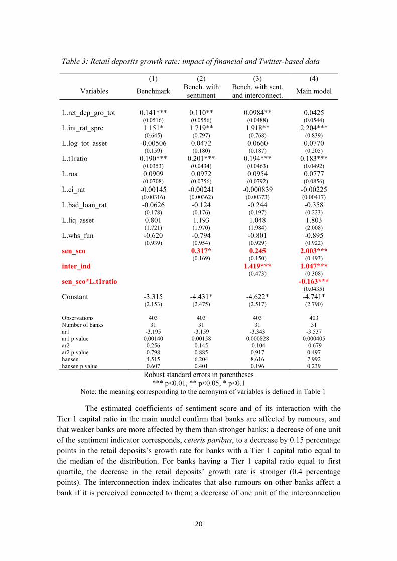
In Table 3 we compare the estimates of the fully-fledged model (1) discussed in section 2 with those of three more contained versions:
1) A benchmark deposits’ growth model without Twitter variables, i.e. the version of (1) where = = = 0 is imposed;
35 See, among others, Nickell 1981, Arellano and Bond 1991, Arellano and Bover 1995, Blundell and Bond 1998. Also see Judson and Owen 1999, Roodman 2006 and Roodman 2008 for an analysis of the technical aspects relative to the implementation of the estimation. 36 The GMM procedure requires the choice of lagged values of endogenous variables as instruments. In our models we have employed lags from 1 to 3. In all specifications, the Sargan – Hansen test produces values greater than 0.05, indicating that we cannot reject the hypothesis of good instruments, underlying the adoption of the GMM estimation procedure. The test for autocorrelation ar2 does not reject the hypothesis of no autocorrelation in residuals, confirming the validity of the specifications adopted.

19
2) A benchmark deposits’ growth model with the addition of the standardized sentiment score, i.e. the version of (1) where = = 0 is imposed;
3) A benchmark deposits’ growth model with the addition of the standardized sentiment score and of the contagion indicator, i.e. the version of (1) where = 0 is imposed.
We will refer to the first model as the “benchmark model” and to the fully-fledged model as the “main model”.
In line with the literature, the benchmark model (see column 1) produces evidence in favour of the market discipline hypothesis. Retail deposits’ growth rate is positively affected by banks’ capitalization level, indicating that retail depositors are able to identify the relative riskiness of banks and tend to prefer relatively safer banks.
The standardized sentiment score shows a slightly positive effect on retail deposits’ growth rate (see column 2), which is consistent with descriptive statistics produced in section 4, suggesting the presence of a positive correlation between sentiment and deposits growth rate (in particular for distressed banks). This indicates that the sentiment indicator proxies the level of alarm among retail depositors regarding specific banks: when rumours circulating on Twitter convey a bad sentiment towards a bank, the retail deposits’ growth rate is negative.
In column 3 we report the results of the version of the model which includes also the interconnection indicator. The effect of this variable is positive, indicating that, when a bank is perceived as connected to banks associated to negative sentiment, it also suffers a decrease in retail deposits. This means that sentiment can not only have a direct effect, but also an indirect effect, impacting on banks not directly involved in negative rumours. This hints to the existence of a channel for contagion dynamics among banks based on the information available to the public and on the sentiment attached to this information. A negative sentiment affects both banks mentioned directly in negative tweets and banks not mentioned in those negative tweets, given that the public perceive the latter as linked to the former.
Estimates for the fully-fledged model are reported in column 4. In this model we introduce a new variable: the interaction term between the standardized sentiment score and the tier1 ratio, which we expect to show that banks are more affected by rumours if their capital ratios is lower.
20
Table 3: Retail deposits growth rate: impact of financial and Twitter-based data
(1) (2) (3) (4)
Variables Benchmark Bench. with sentiment
Bench. with sent. and interconnect.
Main model
L.ret_dep_gro_tot 0.141*** 0.110** 0.0984** 0.0425 (0.0516) (0.0556) (0.0488) (0.0544) L.int_rat_spre 1.151* 1.719** 1.918** 2.204***
(0.645) (0.797) (0.768) (0.839) L.log_tot_asset -0.00506 0.0472 0.0660 0.0770
(0.159) (0.180) (0.187) (0.205) L.t1ratio 0.190*** 0.201*** 0.194*** 0.183***
(0.0353) (0.0434) (0.0463) (0.0492) L.roa 0.0909 0.0972 0.0954 0.0777
(0.0708) (0.0756) (0.0792) (0.0856) L.ci_rat -0.00145 -0.00241 -0.000839 -0.00225
(0.00316) (0.00362) (0.00373) (0.00417) L.bad_loan_rat -0.0626 -0.124 -0.244 -0.358
(0.178) (0.176) (0.197) (0.223) L.liq_asset 0.801 1.193 1.048 1.803
(1.721) (1.970) (1.984) (2.008) L.whs_fun -0.620 -0.794 -0.801 -0.895
(0.939) (0.954) (0.929) (0.922) sen_sco 0.317* 0.245 2.003***
(0.169) (0.150) (0.493) inter_ind 1.419*** 1.047***
(0.473) (0.308) sen_sco*L.t1ratio -0.163***
(0.0435) Constant -3.315 -4.431* -4.622* -4.741*
(2.153) (2.475) (2.517) (2.790)
Observations 403 403 403 403 Number of banks 31 31 31 31 ar1 -3.195 -3.159 -3.343 -3.537 ar1 p value 0.00140 0.00158 0.000828 0.000405 ar2 0.256 0.145 -0.104 -0.679 ar2 p value 0.798 0.885 0.917 0.497 hansen 4.515 6.204 8.616 7.992 hansen p value 0.607 0.401 0.196 0.239
Robust standard errors in parentheses *** p<0.01, ** p<0.05, * p<0.1
Note: the meaning corresponding to the acronyms of variables is defined in Table 1
The estimated coefficients of sentiment score and of its interaction with the Tier 1 capital ratio in the main model confirm that banks are affected by rumours, and that weaker banks are more affected by them than stronger banks: a decrease of one unit of the sentiment indicator corresponds, ceteris paribus, to a decrease by 0.15 percentage points in the retail deposits’s growth rate for banks with a Tier 1 capital ratio equal to the median of the distribution. For banks having a Tier 1 capital ratio equal to first quartile, the decrease in the retail deposits’ growth rate is stronger (0.4 percentage points). The interconnection index indicates that also rumours on other banks affect a bank if it is perceived connected to them: a decrease of one unit of the interconnection

21
indicator corresponds to a decrease by about 1 percentage point in the retail deposits’s growth rate. The other significant coefficients confirm the standard results in the literature about depositor discipline: the variation of retail deposits is positively affected by higher interest rates and higher values of the tier 1 capital ratio.
In table 4 we present a comparison among the mean squared errors of the four models presented above, also separately for distressed and other banks. The main model outperforms the other models37.
Table 4. In sample forecasts comparison across models (Mean of the RMSE for the three main models ;dependent variable: total retail deposits’ growth rate)
Distressed
banks Other banks
Total
Benchmark model 6.6 4.0 4.7
Model augmented with sentiment score 6.2 4.3 4.8
Model augmented with sentiment score and interconnection index
5.9 4.3 4.7
Main model 4.6 4.3 4.4
5.3 Insured and uninsured deposits
In table 5, we present the results relative to two variations of the main model with sentiment and interconnection variables. In the first version, the dependent variable is the total retail deposits’ growth rate, while in the following two models it is represented by the growth rates of uninsured and insured deposits, respectively. As shown by the coefficient associated with the Twitter-based variables, rumours are relevant for both insured and uninsured depositors. The size of the estimated coefficient for uninsured depositors is slightly larger than the corresponding one for insured depositors: for insured depositors, a decrease of one unit of the sentiment indicator corresponds, ceteris paribus, to a decrease in the retail deposits’s growth rate by 0.13 percentage points for banks with a Tier 1 capital ratio equal to the median of the distribution and to a decrease by 0.38 percentage points for banks having a Tier 1 capital ratio equal to first quartile; the decrease becomes, respectively, 0.19 percentage points and 0.47 percentage points if the depositor is uninsured. Looking at the financial data, uninsured depositors seem to monitor more closely credit quality and liquidity,
37 The improvement in the predictions is driven by a strong reduction in the MSE for the distressed banks, indicating that the additional information conveyed by Twitter data is particularly useful in the prediction of distress events interesting distressed banks’ funding. It is interesting to note that, while the MSE of the distressed banks is far bigger than the MSE of the other banks in the benchmark model, the difference almost disappears in the main model.

22
whose coefficients are all significant. These variables, on the other hand, are not statistically significant for insured depositors.
Table 5: Models for guaranteed, unguaranteed and total deposits
(1) (2) (3)
Variables Growth rate of retail
deposits Growth rate of uninsured
retail deposits Growth rate of insured
retail deposits L.ret_dep_gro_tot 0.0425
(0.0544) L. ret_det_gro_unins 0.0846
(0.0645) L. ret_det_gro_ins 0.0498
(0.0510) L.int_rat_spre 2.204*** 2.269** 2.214***
(0.839) (1.051) (0.776) L.log_tot_asset 0.0770 0.0750 0.0945
(0.205) (0.252) (0.190) L.t1ratio 0.183*** 0.210*** 0.168***
(0.0492) (0.0650) (0.0464) L.roa 0.0777 0.0810 0.0669
(0.0856) (0.109) (0.0752) L.ci_rat -0.00225 0.00406 -0.00533
(0.00417) (0.00452) (0.00411) L.bad_loan_rat -0.358 -0.749*** -0.200
(0.223) (0.236) (0.224) L.liq_asset 1.803 4.064* 0.487
(2.008) (2.155) (2.132) L.whs_fun -0.895 -1.423 -0.878
(0.922) (1.175) (0.897) sen_sco 2.003*** 2.200*** 1.922***
(0.493) (0.540) (0.471) inter_ind 1.047*** 1.285*** 0.973***
(0.308) (0.362) (0.298) sen_sco*L.t1ratio -0.163*** -0.176*** -0.157***
(0.0435) (0.0483) (0.0415) Constant -4.741* -5.596 -4.391*
(2.790) (3.492) (2.562) Observations 403 403 403 Number of banks 31 31 31 ar1 -3.537 -3.654 -3.603 ar1 p value 0.000405 0.000258 0.000314 ar2 -0.679 -0.820 -0.474 ar2 p value 0.497 0.412 0.636 hansen 7.992 11.32 7.630 hansen p value 0.239 0.0790 0.267
Robust standard errors in parentheses *** p<0.01, ** p<0.05, * p<0.1
Note: the meaning corresponding to the acronyms of variables is defined in Table 1

23
5.4 Decomposition of the sentiment score
In this section we focus on the sentiment indicator and its components, the volume of attention and the degree of negativity of the period, to study their individual contribution to the prediction improvement. Since the sentiment indicator is defined as the number of negative terms in a period, we can decompose it as
= ∗
where the first term, the number of tweets, represents the volume of attention received by a bank in a period, and the second term – the average sentiment score per tweet – represents the relative negativity of a period given the volume of attention. In the next table, we present a model where each of these three variables (and their interaction with the lagged Tier1) is singularly added to the benchmark model. As for the sentiment score, the number of tweets has been standardized at bank level to prevent scale effects.
As we can see on table 6, all the variables result highly significative. Both the effects, that of the volume of attention and that of the degree of negativity, seem to be by themselves important predictors for the variation of retail deposits: for banks having a Tier 1 capital ratio equal to the median, an increase of 1 per cent in the standardised number of tweets leads to a decrease by 0.25 percentage points in the retail deposits’ growth rate, and an increase of 10 per cent in the negative ratio leads to a decrease by 0.03 percentage points in the retail deposits’ growth rate.

24
Table 6: Sentiment indicator, number of tweets and negative ratio
(1) (2) (3) Variables Standardized sentiment
score Standardized number
of tweets Negative ratio
L.ret_dep_gro_tot 0.898 0.744 0.117
(0.655) (0.601) (0.591) L.cr_torr -1.055 -0.904 0.146
(0.823) (0.765) (0.650) L.int_rat_spre 2.151* 2.170* 1.966**
(1.122) (1.169) (0.903) L.log_tot_asset 0.0263 0.0209 0.161
(0.213) (0.212) (0.167) L.t1ratio 0.237*** 0.238*** 0.184***
(0.0687) (0.0624) (0.0580) L.roa 0.0287 0.0408 0.0969
(0.0909) (0.0894) (0.0893) L.ci_rat -0.00544 -0.00512 0.00183
(0.00495) (0.00513) (0.00333) L.bad_loan_rat -0.305 -0.293 -0.308
(0.235) (0.243) (0.194) L.liq_asset 3.357 2.686 2.583
(2.174) (1.989) (1.872) L.whs_fun -0.0926 -0.271 0.192
(1.073) (0.994) (0.707) sen_sco 2.514***
(0.671) sen_sco*L.t1ratio -0.203***
(0.0599) tweet_std -2.446***
(0.673) tweet_std*L.t1ratio 0.192***
(0.0570) neg_ratio -0.0379***
(0.0143) neg_ ratio * L.t1ratio 0.00305***
(0.00110) Constant -5.516 -5.332 -6.280***
(3.434) (3.358) (2.409) Observations 403 403 296 Number of banks 31 31 31 ar1 -3.371 -3.400 -2.594 ar1 p value 0.000749 0.000674 0.00947 ar2 0.495 0.634 1.000 ar2 p value 0.620 0.526 0.317 hansen 3.363 5.727 9.765 hansen p value 0.644 0.334 0.0822
Robust standard errors in parentheses *** p<0.01, ** p<0.05, * p<0.1
Note: the meaning corresponding to the acronyms of variables is defined in Table 1

25
6. Conclusions In this paper we explore the use of Twitter data for the study of banks’ funding.
Twitter data is analysed to extract information regarding the sentiment and the perceived interconnection of banks. A benchmark market discipline model used for the prediction of retail deposits’ growth rate and the same model augmented with sentiment and interconnection variables are separately estimated. We find that information derived from Twitter significantly improves the explanatory and forecasting power of the benchmark market discipline model: in particular, a negative sentiment corresponds, ceteris paribus, to lower retail deposits growth rates. We also find that depositors of distressed banks tend to be more responsive than the other depositors to bad rumours. These findings contribute to extend the range of the applications of Twitter data for the forecasting of financial data presently available in the literature.
We also elaborate an original method to exploit Twitter data to construct an indicator able to capture informational spillover effects across banks. Textual content is directly analysed both to gather a quantitative measure of how much banks are perceived as interconnected and to capture the way sentiment towards one bank can influence other banks. We show that a bank’s retail deposits growth rate is affected by the sentiment towards other banks, with which the bank is perceived to be connected. This finding contributes to the understanding of “informational contagion” dynamics across banks and motivates the use of Twitter data for the study and the monitoring of interconnections in the banking system.
From a policy perspective, this study allows to disentangle the effects of bank-specific versus industry-wide informative contagion. The significance of both our indicators (the sentiment and the interconnectedness indicator) suggests that both channels of contagion are at work, and that information spillover across banks should not be underplayed, including by policymakers. At the same time, the findings confirm that information about banks’ fundamentals retains the capacity to correctly drive depositor’s choices. This is shown by, first, the weaker explanatory power of social media-related indicators on deposit flows of sounder banks, and, second, by the attenuation of their impact for highly capitalised banks.

26
7. Appendices
7.1 Estimation of the uninsured amount of Italian retail deposits
The estimation of the uninsured amount of Italian retail deposits presents two problems:
1) Data present number of depositors and amount of deposits divided by amount class with only three main classes available: deposits below 50.000 euro, deposits between 50.000 and 250.000 euro and deposits above 250.000 euro. While the uninsured amount for the first and the last class can be deterministically computed, the exact uninsured amount for the middle class is not known.
2) Data divided by amount class are available only on a semi-annual basis.
We solve the problems in a three-step way. First, for each bank, we compute the semi-annual ratio of uninsured deposits on total deposits with the methodology reported below. Then, we interpolate between the semi-annual ratios to obtain a monthly ratio of uninsured deposits. Finally, we apply the ratio to the available monthly data on total deposits to obtain the monthly stock of uninsured (and thus insured) deposits.
To compute the uninsured amount of retail deposits of a bank for the class of deposits between 50.000 euro and 250.000 euro, first we divide the data using the highest possible granularity of the dataset (e.g. dividing by province class); then, we estimate for each of these subsets the lowest and the highest possible uninsured amount in deposits given the number of depositors and the total amount; finally, we sum up across all subsets the highest possibile uninsured amounts obtained, and we use it as an estimation for the uninsured deposits. This methodology gives the optimal worst-possible case for the amount of uninsured deposits in the class.
Driven by the necessity of estimating the uninsured amount of retail deposits in the class 50.000 euro - 250.000 euro when only the number of depositors and the total amount is known, we generalize the problem in the following way.
Let , , be real numbers, with < < ; and will be the extremes of the admittable values, and the threshold (in the uninsured deposits case, = 50.000, = 250.000 and = 100.000). We have a set of measures { , … , } such that < < ∀ = 1,… , , of which we know only their total number and their total sum =∑ x .

27
We are interested in finding an optimal bound for the sum of the amounts of exceeding , i.e.
= y , (2)
where y = max(0, − ). We’ll call y the Exceeding Amount. In this section, we’ll prove that the Exceeding Amount satisfies max 0, ( − ) ≤ ≤ (b − k)n +max (0, (1 − ) + − ),
(3)
where (the mean) is defined in Theorem 1 and and are defined in Theorem 2, and that such bound is optimal, that is there can’t be a better deterministic bound. We divide the proof in two theorems, respectively for the lower bound and the upper bound.
Theorem 1 (Lower Bound).
Let = = ∑ be the mean of the measures. Then, the Exceeding Amount
verifies ≥ max 0, ( − ) , (4)
and the bound is optimal.
Proof of Theorem 1.
We want to show that the configuration having all measures equal to the mean gives the minimal Exceeding Amount (E.A.), and, since the E.A. of this configuration is max 0, ( − ) , we’ll have proven the bound defined in Theorem 1 (moreover, since
it is the E.A. of a possible configuration, the bound will be optimal).
Let { , … , } be a configuration such that ∑ = , where not all measures are equal to μ. Then, if we prove that exists a configuration { ′ , … , ′ } such that the number of measures equal to the mean is strictly greater, such that ∑ =∑ = and such that the E.A. is lower or equal the E.A. of the starting

28
configuration, the thesis will follow by iterating the process, to any possible configuration, until all measures are equal to the mean.
Without loss of generality, let , be such that < < (since the average is and not all the measures are equal to , there must exist a measure greater than the mean and a measure lower than the mean), and let’s define a new configuration where all the measures except and are equal to those in the initial configuration, and where we replace and with = and = + − . Then:
1) ∑ = ∑ = , since by construction + = + ; 2) The number of measures equal to the mean in the new configuration is strictly
greater, because = (while , ≠ ); 3) The Exceeding Amount of the new configuration is less or equal than the E.A.
of the initial one, because − = − and > , that implies that the
E.A. lost by , max 0, ( − ) −max 0, ( − ) = 0, is greater or equal
than the E.A. gained by ,that is max 0, ( − ) −max 0, ( − ) . Thus, the thesis follow.
Proposition 1.
The Exceeding Amount is maximal when all the measures (except at most one) are equal to either or . We’ll call this configuration the Maximal Configuration.
Theorem 2 (Upper Bound).
Let = = ∑ be the mean of the measures, = ( ⋅ ( )) and
= ⋅ ( ) − . Then, the Exceeding Amount verifies
≤ (b − k)n + max (0, (1 − ) + − ), (5)
and the bound is optimal. Proof of Theorem 2.
Let’s assume Proposition 1 true (we’ll prove it later). Thus, the Exceeding Amount is maximal when all the measures (except at most one) are equal to either a or b, i.e. in the Maximal Configuration, and we only have to show the E.A. of this configuration is equal to the right side of the formula in Theorem 2. We divide the proof in two cases.

29
1. The Maximal Configuration has only deposits equal to or . In this case, solving the linear system: ⋅ = ⋅ + ⋅ = + ,
we obtain the unique solution where we have = ⋅ deposits
equal to and = ⋅ deposits equal to . Since the solution is unique and
we are in case 1, and must be integer, though the solution is a valid configuration, is equal to 0 (because it is the fractional part of an integer number) and the maximal amount, obtained counting simply the maximal amount of the deposits equal to b, is equal to (b − k) = (b − k) ,
that is the thesis.
2. The maximal configuration has one deposit different from and . Let’s define
and as in the proposition of Theorem 2, that is = ( ⋅ ( )) and
= ⋅ ( ) − . First we notice that, since by definition + = − − is integer and 0 < , < 1 (the left inequality because we’re in case 2, and
the right inequality because they’re fractionary parts), we have that + = 1, i.e. = 1 − . It now follows, simply substituting the values, that the configuration with deposits equal to , deposits equal to and one deposit equal to + = (1 − ) + is the Maximal Configuration, because + + 1 = and + + (1 − ) + = ⋅ . The thesis follows from the fact that the Exceeding Amount of this configuration is equal to:
(b − k)n + max(0, (1 − ) + − ), where the first term is given by the n deposits equal to b and the last
term from the deposit equal to (1 − ) + .
Proof of Proposition 1.
Analogously to what we have done in the proof of Theorem 1, let’s show that, given an initial configuration { , … , }such that at least two of the measures are different from both and , there is a configuration, with the same total value, such that the number of measures equals to or is strictly greater than their number in the

30
initial configuration, and such that the Exceeding Amount (E.A.) is greater or equal than the E.A. of the initial configuration.
Without loss of generality, let < < < . Such measures exist by definition of the initial configuration. We differentiate two cases:
1) − ≤ − ; In this case, we define = and = + ( − ). Since we’re in
case (1), by construction ≤ and the configuration is a valid one. Moreover, the Exceeding Amount of the new configuration minus the E.A. of the initial one is equal to ( ) − ( ) = (max( − , 0) + max( − , 0)) − (max( − , 0) −max( − , 0))= (max( − , 0) − max( − , 0)) − (max( − , 0) −max( , 0)),
which is ≥ 0 because − = − and ≥ , though the
exceeding amount can only be greater (the E.A. gained from is greater or equal than the E.A. lost by ).
2) − > − ; In this case, we define = and = − ( − ) and we proceed
analogously.
Iterating the process we find that, given any initial configuration, there is always a configuration with at most one measure different from both and and such that its Exceeding Amount is greater or equal than the E.A. of the initial configuration, i.e. the thesis.
7.2 Computation of the indicator of perceived interconnection between banks
Twitter data provide the possibility of mapping the perceived interconnections between banks. Similarly to market returns, Twitter provides information on the way attention on a particular bank co-moves with the attention on another one. Unlike market data, Twitter data are un-structured and somewhat qualitative data, that need to be translated in numeric values in order to calculate correlation matrices and similar measures. Of the possible approaches for the construction of an indicator of

31
interconnection38, in this paper we implement one based on the simultaneous occurrence of different banks in the same tweet. Every bank in any period of time (month) is characterised by a vector: = , , , … … , , , ,
where = , is the number of tweets on the nth bank, N is the total number
of banks and , , … , , are the numbers of tweets regarding the nth bank that
contain reference to the banks 1 to N. The conditional probability for the ith bank of been referenced to in tweets regarding the nth bank is then defined as:
, = , . = [ , , … , , ] is used as a vector of weights for the computation of the
interconnection index. The bank specific vector , omitting the nth element, is multiplied by the vector containing the standardized sentiment score for all banks different from the nth bank. The nth element is omitted because in the econometric analysis the sentiment score for the nth bank is analysed in a separate variable and thus the inclusion of the nth element in the following summation would produce a duplication. Formally, the interconnection index is defined as: _ = , ∗∈ | ,
where , is defined above and is the standardized sentiment score for bank
i. The interconnection index is then employed as explanatory variable together with the sentiment score at a bank-period level. While the standardized sentiment score aims at capturing the general sentiment towards a single bank, the indicator of interconnection represents the sentiment on other banks weighted by the degree of perceived interconnection these other banks have with the bank under examination.
38 See, for instance, P. Cerchiello, P. Giudici, C. Nicola 2016, where the correlation between banks is derived from the correlation of Twitter-based time series of daily “mood-returns” (that weekly, but positively, correlate to the corresponding market returns).

32
7.3 Comparison of OLS, Fixed Effects and GMM estimators
As a robustness check of the results, in this appendix we compare the GMM estimates with the OLS and the Fixed Effects estimates. While both the OLS and the Fixed Effects estimators are supposed to be biased due, respectively, to bank level fixed effect and to the lagged dependent variable (see subsection 5.1 for more details), the F.E. results for the exogenous variables weakly correlated with them – in particular, the significance for the Twitter-based variables – should be only partially affected by the choice of the estimation method. We compare the results for the three main social variables (sentiment score, contagion indicator and interaction between sentiment score and tier1 ratio) calculated using three different estimators: an OLS estimator, a F.E. estimator and our GMM estimator. As we can see on Table 7 below, the coefficients are pretty close and the high significance appears to hold throughout all the estimation methods.

33
Table 7: Comparison of OLS, Fixed Effects and GMM estimators
(1) (2) (3)
Variables OLS Fixed Effects GMM
L.ret_dep_gro_tot 0.142 -0.0168 0.0425
(0.0951) (0.0692) (0.0544) L.int_rat_spre 0.699* 1.732*** 2.204***
(0.363) (0.520) (0.839) L.log_tot_asset -0.0995 2.655 0.0770
(0.131) (2.267) (0.205) L.t1ratio 0.149*** 0.297*** 0.183***
(0.0316) (0.0807) (0.0492) L.roa 0.0239 0.0950 0.0777
(0.0509) (0.111) (0.0856) L.ci_rat 0.00299 0.000138 -0.00225
(0.00435) (0.00572) (0.00417) L.bad_loan_rat -0.354 -0.217 -0.358
(0.232) (0.459) (0.223) L.liq_asset 1.444 -0.298 1.803
(1.145) (6.080) (2.008) L.whs_fun -0.222 -1.701 -0.895
(0.678) (2.760) (0.922) sen_sco 1.767*** 1.868*** 2.003***
(0.460) (0.546) (0.493) inter_ind 0.882*** 0.785** 1.047***
(0.246) (0.309) (0.308) sen_sco*L.t1ratio -0.148*** -0.158*** -0.163***
(0.0401) (0.0466) (0.0435) Constant -1.354 -31.43 -4.741*
(1.540) (22.01) (2.790)
Observations 403 403 403 R-squared 0.289 0.237 Number of banks 31 31 ar1 -3.537 ar1 p value 0.000405 ar2 -0.679 ar2 p value 0.497 hansen 7.992 hansen p value 0.239
Robust standard errors in parentheses *** p<0.01, ** p<0.05, * p<0.1
Note: the meaning corresponding to the acronyms of variables is defined in Table 1.

34
References
Acharya, V. and Mora, N. (2012), “Are Banks Passive Liquidity Backstops? Deposit Rates and Flows During the 2007-2009 Crisis”, Nber Working Paper.
Arellano, M. and Bond, S. (1991), “Some tests of specification for panel data: Monte Carlo evidence and an application to employment equations”, Review of Economic Studies, Vol. 58, 277–297.
Arellano, M. and Bover, O. (1995), “Another look at the instrumental variables estimation of error components models”, Journal of Econometrics, Vol. 68, 29–51.
Arnold, E.A., Größl, I. and Koziol, P. (2016), “Market Discipline across Bank Governance Models: Empirical Evidence from German Depositors”, The Quarterly Review of Economics and Finance, 61, 126-138.
Baer, H. and Brewer, E. (1986), Uninsured Deposits as a Source of Market Discipline: Some New Evidence, Federal Reserve Bank of Chicago, Economic Perspectives.
Benoit, S., Colliard, J.-E., Hurlin, C. and Pérignon, C. (2015), “Where the Risk Lie: a Survey on Systemic Risk”, HAL Archives Ouvert.
Bikker, J.A. (2003), “Testing for imperfect competition on EU deposit and loan markets with Bresnahan’s market power model”, De Nederlandsche Bank, Research Series Supervision no. 52.
Blundell, R. and Bond, S. (1998), “Initial conditions and moment restrictions in dynamic panel data models”, Journal of Econometrics, Vol. 87, 115–143.
Bollen, J., Mao, H., and Zeng, X.J. (2011), “Twitter mood predicts the stock market”, Journal of Computational Science, Vol. 2, Issue 1, 1-8.
Bordino, I., Battiston S., Caldarelli G., Cristelli M. and Ukkonen A. (2012), “Web Search Queries Can Predict Stock Market Volumes”, PLoS ONE, vol. 7, iss. 7.
Bresnahan, T.F. (1982), “The Oligopoly Solution Concept is Identified”, Economic Letters, 10.
Cerchiello, P., Giudici, P. and Nicola, G. (2016), “Big Data Models of Bank Risk Contagion”, DEM Working Paper Series, 117.
D’Amuri, F. and Marcucci, J. (2017), “The Predictive Power of Google Searches in Forecasting US Unemployment”, International Journal of Forecasting, October-December, 33(4), 801-816.
Da, Z., Engelberg, J. and Gao, P. (2011), “In Search of Attention”, The Journal of Finance – Vol. LXVI, No.5, October 2011.

35
Dickinson, B. and Hu, W. (2015), “Sentiment analysis of investor opinions on Twitter”, Social Networking, 4, 62-71.
Ferguson, N.J., Philip, D., Lam, H.Y.T. and Guo, J.M. (2015), “Media Content and Stock Returns: The Predictive Power of the Press”, Multinational Finance Journal, Vol. 19, No. 1, 1–31.
Hájek P. and Olej V. (2013), “Evaluating Sentiment in Annual Reports for Financial Distress Prediction Using Neural Networks and Support Vector Machines”, EANN 2013: Engineering Applications of Neural Networks pp 1-10.
Hamada, M. (2011), “Market Discipline by Depositors: Impact of Deposit Insurance on the Indonesian Banking Sector”, Institute of Developing Economies, Discussion Papers.
Hasan, I., Jakowicz, K., Kowalewski, O. and Kozlowski, L (2013), “Market discipline during crisis: Evidence from bank depositors in transition countries”, Journal of Banking & Finance, Vol. 37.
Iyer, R. and Puri, M. (2012), “Understanding Bank Runs: The Importance of Depositor-Bank Relationships and Networks”, American Economic Review, 102 (4), 1414-1445.
Judson, R.A. and Owen, A.L. (1999), “Estimating dynamic panel data models: a guide for macroeconomists”, Economic Letters, 65, 9-15.
Kearney, C. and Liu, S. (2014), “Textual sentiment in finance: A survey of methods and models”, International Review of Financial Analysis, 33.
Lerman, K. and Ghosh, R. (2010), Information Contagion: an Empirical Study of the Spread of News on Digg and Twitter Social Networks, Proceedings of the Fourth International AAAI Conference on Weblogs and Social Media.
Li, F. (2006), “Do stock market investors understand the risk sentiment of corporate annual reports?”, Available at SSRN: https://ssrn.com/abstract=898181
Loughran, T., and McDonald, B. (2011), “When is a liability not a liability?”, The Journal of Finance, Vol. 66, Issue 1, 35-65.
Maechler A.M. and McDill, K.M. (2006), Dynamic depositor discipline in US banks, Journal of Banking & Finance, Vol 30.
Mao, H., Counts, S. and Bollen, J. (2015), “Quantifying the effects of online bullishness on international financial markets”, ECB Statistics Paper No 9, July 2015.
Nickell S. (1981), “Biases in Dynamic Models with Fixed Effects”, Econometrica, 49, 6, pp.1417-1426.

36
Nopp, C. and Hanbury, A. (2015), “Detecting Risks in the Banking System by Sentiment Analysis”, Proceedings of the 2015 Conference on Empirical Methods in Natural Language Processing.
Nyman, R., Gregory, D., Kapadia, S.,Ormerod, P., Tuckett, D. and Smith, R. (2018), “News and narratives in financial systems: Exploiting big data for systemic risk assessment”, Bank of England Working Paper.
Park, S. (1995), Market Discipline by Depositors: Evidence from Reduced Form Equations, The Federal bank of Saint Louis, Working Paper Series.
Park, S., and Peristiani, S. (1998). Market Discipline by Thrift Depositors. Journal of Money Credit and Banking, 30, 347-364.
Peria, M.S. and Schmukler, S.L. (2001), Do Depositors Punish Banks for Bad Behaviour? Market Discipline, Deposit Insurance, and Banking Crises, The Journal of Finance Vol 56, No. 3.
Roodman, D. (2006), “How to do xtabond2: an introduction to ‘difference’ and ‘system’ GMM in Stata”, Center for Global Development Working Paper, 103.
Roodman, D. (2008), “A Note on the Theme of Too Many Instruments”, Center for Global Development Working Paper, 125.
Shimizu K. (2009), “Is the Information Produced in the Stock Market Useful for Depositors?”, Finance Research Letters, vol. 6, 34-39.
Tetlock, P.C. (2007) “Giving content to investor sentiment: The role of media in the stock market”, The Journal of Finance, Vol. LXII, No. 3.

(*) Requests for copies should be sent to: Banca d’Italia – Servizio Studi di struttura economica e finanziaria – Divisione Biblioteca e Archivio storico – Via Nazionale, 91 – 00184 Rome – (fax 0039 06 47922059). They are available on the Internet www.bancaditalia.it.
RECENTLY PUBLISHED “TEMI” (*)
N. 1149 – Looking behind the financial cycle: the neglected role of demographics, by Alessandro Ferrari (December 2017).
N. 1150 – Public investment and monetary policy stance in the euro area, by Lorenzo Burlon, Alberto Locarno, Alessandro Notarpietro and Massimiliano Pisani (December 2017).
N. 1151 – Fiscal policy uncertainty and the business cycle: time series evidence from Italy, by Alessio Anzuini, Luca Rossi and Pietro Tommasino (December 2017).
N. 1152 – International financial flows and the risk-taking channel, by Pietro Cova and Filippo Natoli (December 2017).
N. 1153 – Systemic risk and systemic importance measures during the crisis, by Sergio Masciantonio and Andrea Zaghini (December 2017).
N. 1154 – Capital controls, macroprudential measures and monetary policy interactions in an emerging economy, by Valerio Nispi Landi (December 2017).
N. 1155 – Optimal monetary policy and fiscal policy interaction in a non-Ricardian economy, by Massimiliano Rigon and Francesco Zanetti (December 2017).
N. 1156 – Secular stagnation, R&D, public investment and monetary policy: a global-model perspective, by Pietro Cova, Patrizio Pagano, Alessandro Notarpietro and Massimiliano Pisani (December 2017).
N. 1157 – The CSPP at work: yield heterogeneity and the portfolio rebalancing channel, by Andrea Zaghini (December 2017).
N. 1158 – Targeting policy-compliers with machine learning: an application to a tax rebate programme in Italy, by Monica Andini, Emanuele Ciani, Guido de Blasio, Alessio D’Ignazio and Viola Salvestrini (December 2017).
N. 1159 – Banks’ maturity transformation: risk, reward, and policy, by Pierluigi Bologna (December 2017).
N. 1160 – Pairwise trading in the money market during the European sovereign debt crisis, by Edoardo Rainone (December 2017).
N. 1140 – Natural rates across the Atlantic, by Andrea Gerali and Stefano Neri (September 2017).
N. 1141 – A quantitative analysis of risk premia in the corporate bond market, by Sara Cecchetti (October 2017).
N. 1142 – Monetary policy in times of debt, by Mario Pietrunti and Federico M. Signoretti (October 2017).
N. 1143 – Capital misallocation and financial development: a sector-level analysis, by Daniela Marconi and Christian Upper (October 2017).
N. 1144 – Leaving your mamma: why so late in Italy?, by Enrica Di Stefano (October 2017).
N. 1145 – A Financial Conditions Index for the CEE economies, by Simone Auer (October 2017).
N. 1146 – Internal capital markets in times of crisis: the benefit of group affiliation in Italy, by Raffaele Santioni, Fabio Schiantarelli and Philip E. Strahan (October 2017).
N. 1147 – Consistent inference in fixed-effects stochastic frontier models, by Federico Belotti and Giuseppe Ilardi (October 2017).
N. 1148 – Investment decisions by European firms and financing constraints, by Andrea Mercatanti, Taneli Mäkinen and Andrea Silvestrini (October 2017).
N. 1161 – Please in my back yard: the private and public benefitsof a new tram line in Florence, by Valeriia Budiakivska and Luca Casolaro (January 2018).
N. 1162 – Real exchange rate misalignments in the euro area, by by Michael Fidora, Claire Giordano and Martin Schmitz (January 2018).
N. 1163 – What will Brexit mean for the British and euro-area economies? A model-based assessment of trade regimes, by Massimiliano Pisani and Filippo Vergara Caffarelli (January 2018).
N. 1164 – Are lenders using risk-based pricing in the consumer loan market? The effects of the 2008 crisis, by Silvia Magri (January 2018).

"TEMI" LATER PUBLISHED ELSEWHERE
2016
ALBANESE G., G. DE BLASIO and P. SESTITO, My parents taught me. evidence on the family transmission of values, Journal of Population Economics, v. 29, 2, pp. 571-592, TD No. 955 (March 2014).
ANDINI M. and G. DE BLASIO, Local development that money cannot buy: Italy’s Contratti di Programma, Journal of Economic Geography, v. 16, 2, pp. 365-393, TD No. 915 (June 2013).
BARONE G. and S. MOCETTI, Inequality and trust: new evidence from panel data, Economic Inquiry, v. 54, pp. 794-809, TD No. 973 (October 2014).
BELTRATTI A., B. BORTOLOTTI and M. CACCAVAIO, Stock market efficiency in China: evidence from the split-share reform, Quarterly Review of Economics and Finance, v. 60, pp. 125-137, TD No. 969 (October 2014).
BOLATTO S. and M. SBRACIA, Deconstructing the gains from trade: selection of industries vs reallocation of workers, Review of International Economics, v. 24, 2, pp. 344-363, TD No. 1037 (November 2015).
BOLTON P., X. FREIXAS, L. GAMBACORTA and P. E. MISTRULLI, Relationship and transaction lending in a crisis, Review of Financial Studies, v. 29, 10, pp. 2643-2676, TD No. 917 (July 2013).
BONACCORSI DI PATTI E. and E. SETTE, Did the securitization market freeze affect bank lending during the financial crisis? Evidence from a credit register, Journal of Financial Intermediation , v. 25, 1, pp. 54-76, TD No. 848 (February 2012).
BORIN A. and M. MANCINI, Foreign direct investment and firm performance: an empirical analysis of Italian firms, Review of World Economics, v. 152, 4, pp. 705-732, TD No. 1011 (June 2015).
BRAGOLI D., M. RIGON and F. ZANETTI, Optimal inflation weights in the euro area, International Journal of Central Banking, v. 12, 2, pp. 357-383, TD No. 1045 (January 2016).
BRANDOLINI A. and E. VIVIANO, Behind and beyond the (headcount) employment rate, Journal of the Royal Statistical Society: Series A, v. 179, 3, pp. 657-681, TD No. 965 (July 2015).
BRIPI F., The role of regulation on entry: evidence from the Italian provinces, World Bank Economic Review, v. 30, 2, pp. 383-411, TD No. 932 (September 2013).
BRONZINI R. and P. PISELLI, The impact of R&D subsidies on firm innovation, Research Policy, v. 45, 2, pp. 442-457, TD No. 960 (April 2014).
BURLON L. and M. VILALTA-BUFI, A new look at technical progress and early retirement, IZA Journal of Labor Policy, v. 5, TD No. 963 (June 2014).
BUSETTI F. and M. CAIVANO, The trend–cycle decomposition of output and the Phillips Curve: bayesian estimates for Italy and the Euro Area, Empirical Economics, V. 50, 4, pp. 1565-1587, TD No. 941 (November 2013).
CAIVANO M. and A. HARVEY, Time-series models with an EGB2 conditional distribution, Journal of Time Series Analysis, v. 35, 6, pp. 558-571, TD No. 947 (January 2014).
CALZA A. and A. ZAGHINI, Shoe-leather costs in the euro area and the foreign demand for euro banknotes, International Journal of Central Banking, v. 12, 1, pp. 231-246, TD No. 1039 (December 2015).
CESARONI T. and R. DE SANTIS, Current account “core-periphery dualism” in the EMU, The World Economy, v. 39, 10, pp. 1514-1538, TD No. 996 (December 2014).
CIANI E., Retirement, Pension eligibility and home production, Labour Economics, v. 38, pp. 106-120, TD No. 1056 (March 2016).
CIARLONE A. and V. MICELI, Escaping financial crises? Macro evidence from sovereign wealth funds’ investment behaviour, Emerging Markets Review, v. 27, 2, pp. 169-196, TD No. 972 (October 2014).
CORNELI F. and E. TARANTINO, Sovereign debt and reserves with liquidity and productivity crises, Journal of International Money and Finance, v. 65, pp. 166-194, TD No. 1012 (June 2015).
D’AURIZIO L. and D. DEPALO, An evaluation of the policies on repayment of government’s trade debt in Italy, Italian Economic Journal, v. 2, 2, pp. 167-196, TD No. 1061 (April 2016).
DE BLASIO G., G. MAGIO and C. MENON, Down and out in Italian towns: measuring the impact of economic downturns on crime, Economics Letters, 146, pp. 99-102, TD No. 925 (July 2013).
DOTTORI D. and M. MANNA, Strategy and tactics in public debt management, Journal of Policy Modeling, v. 38, 1, pp. 1-25, TD No. 1005 (March 2015).

LIBERATI D., M. MARINUCCI and G. M. TANZI, Science and technology parks in Italy: main features and analysis of their effects on hosted firms, Journal of Technology Transfer, v. 41, 4, pp. 694-729, TD No. 983 (November 2014).
MARCELLINO M., M. PORQUEDDU and F. VENDITTI, Short-Term GDP forecasting with a mixed frequency dynamic factor model with stochastic volatility, Journal of Business & Economic Statistics , v. 34, 1, pp. 118-127, TD No. 896 (January 2013).
RODANO G., N. SERRANO-VELARDE and E. TARANTINO, Bankruptcy law and bank financing, Journal of Financial Economics, v. 120, 2, pp. 363-382, TD No. 1013 (June 2015).
ZINNA G., Price pressures on UK real rates: an empirical investigation, Review of Finance,v. 20, 4, pp. 1587-1630, TD No. 968 (July 2014).
2017
ADAMOPOULOU A. and G.M. TANZI, Academic dropout and the great recession, Journal of Human Capital, V. 11, 1, pp. 35–71, TD No. 970 (October 2014).
ALBERTAZZI U., M. BOTTERO and G. SENE, Information externalities in the credit market and the spell of credit rationing, Journal of Financial Intermediation, v. 30, pp. 61–70, TD No. 980 (November 2014).
ALESSANDRI P. and H. MUMTAZ, Financial indicators and density forecasts for US output and inflation, Review of Economic Dynamics, v. 24, pp. 66-78, TD No. 977 (November 2014).
BARBIERI G., C. ROSSETTI and P. SESTITO, Teacher motivation and student learning, Politica economica/Journal of Economic Policy, v. 33, 1, pp.59-72, TD No. 761 (June 2010).
BENTIVOGLI C. and M. LITTERIO, Foreign ownership and performance: evidence from a panel of Italian firms, International Journal of the Economics of Business, v. 24, 3, pp. 251-273, TD No. 1085 (October 2016).
BRONZINI R. and A. D’IGNAZIO, Bank internationalisation and firm exports: evidence from matched firm-bank data, Review of International Economics, v. 25, 3, pp. 476-499 TD No. 1055 (March 2016).
BRUCHE M. and A. SEGURA, Debt maturity and the liquidity of secondary debt markets, Journal of Financial Economics, v. 124, 3, pp. 599-613, TD No. 1049 (January 2016).
BURLON L., Public expenditure distribution, voting, and growth, Journal of Public Economic Theory,, v. 19, 4, pp. 789–810, TD No. 961 (April 2014).
BURLON L., A. GERALI, A. NOTARPIETRO and M. PISANI, Macroeconomic effectiveness of non-standard monetary policy and early exit. a model-based evaluation, International Finance, v. 20, 2, pp.155-173, TD No. 1074 (July 2016).
BUSETTI F., Quantile aggregation of density forecasts, Oxford Bulletin of Economics and Statistics, v. 79, 4, pp. 495-512, TD No. 979 (November 2014).
CESARONI T. and S. IEZZI, The predictive content of business survey indicators: evidence from SIGE, Journal of Business Cycle Research, v.13, 1, pp 75–104, TD No. 1031 (October 2015).
CONTI P., D. MARELLA and A. NERI, Statistical matching and uncertainty analysis in combining household income and expenditure data, Statistical Methods & Applications, v. 26, 3, pp 485–505, TD No. 1018 (July 2015).
D’AMURI F. and J. MARCUCCI, The predictive power of google searches in forecasting unemployment, International Journal of Forecasting, v. 33, 4, pp. 801-816, TD No. 891 (November 2012).
DE BLASIO G. and S. POY, The impact of local minimum wages on employment: evidence from Italy in the 1950s, Journal of Regional Science, v. 57, 1, pp. 48-74, TD No. 953 (March 2014).
DEL GIOVANE P., A. NOBILI and F. M. SIGNORETTI, Assessing the sources of credit supply tightening: was the sovereign debt crisis different from Lehman?, International Journal of Central Banking, v. 13, 2, pp. 197-234, TD No. 942 (November 2013).
DEL PRETE S., M. PAGNINI, P. ROSSI and V. VACCA, Lending organization and credit supply during the 2008–2009 crisis, Economic Notes, v. 46, 2, pp. 207–236, TD No. 1108 (April 2017).
DELLE MONACHE D. and I. PETRELLA, Adaptive models and heavy tails with an application to inflation forecasting, International Journal of Forecasting, v. 33, 2, pp. 482-501, TD No. 1052 (March 2016).
LOBERTO M. and C. PERRICONE, Does trend inflation make a difference?, Economic Modelling, v. 61, pp. 351–375, TD No. 1033 (October 2015).

MANCINI A.L., C. MONFARDINI and S. PASQUA, Is a good example the best sermon? Children’s imitation of parental reading, Review of Economics of the Household, v. 15, 3, pp 965–993, D No. 958 (April 2014).
MEEKS R., B. NELSON and P. ALESSANDRI, Shadow banks and macroeconomic instability, Journal of Money, Credit and Banking, v. 49, 7, pp. 1483–1516, TD No. 939 (November 2013).
MICUCCI G. and P. ROSSI, Debt restructuring and the role of banks’ organizational structure and lending technologies, Journal of Financial Services Research, v. 51, 3, pp 339–361, TD No. 763 (June 2010).
MOCETTI S., M. PAGNINI and E. SETTE, Information technology and banking organization, Journal of Journal of Financial Services Research, v. 51, pp. 313-338, TD No. 752 (March 2010).
MOCETTI S. and E. VIVIANO, Looking behind mortgage delinquencies, Journal of Banking & Finance, v. 75, pp. 53-63, TD No. 999 (January 2015).
NOBILI A. and F. ZOLLINO, A structural model for the housing and credit market in Italy, Journal of Housing Economics, v. 36, pp. 73-87, TD No. 887 (October 2012).
PALAZZO F., Search costs and the severity of adverse selection, Research in Economics, v. 71, 1, pp. 171-197, TD No. 1073 (July 2016).
PATACCHINI E. and E. RAINONE, Social ties and the demand for financial services, Journal of Financial Services Research, v. 52, 1–2, pp 35–88, TD No. 1115 (June 2017).
PATACCHINI E., E. RAINONE and Y. ZENOU, Heterogeneous peer effects in education, Journal of Economic Behavior & Organization, v. 134, pp. 190–227, TD No. 1048 (January 2016).
SBRANA G., A. SILVESTRINI and F. VENDITTI, Short-term inflation forecasting: the M.E.T.A. approach, International Journal of Forecasting, v. 33, 4, pp. 1065-1081, TD No. 1016 (June 2015).
SEGURA A. and J. SUAREZ, How excessive is banks' maturity transformation?, Review of Financial Studies, v. 30, 10, pp. 3538–3580, TD No. 1065 (April 2016).
VACCA V., An unexpected crisis? Looking at pricing effectiveness of heterogeneous banks, Economic Notes, v. 46, 2, pp. 171–206, TD No. 814 (July 2011).
VERGARA CAFFARELI F., One-way flow networks with decreasing returns to linking, Dynamic Games and Applications, v. 7, 2, pp. 323-345, TD No. 734 (November 2009).
ZAGHINI A., A Tale of fragmentation: corporate funding in the euro-area bond market, International Review of Financial Analysis, v. 49, pp. 59-68, TD No. 1104 (February 2017).
2018
CARTA F. and M. DE PHLIPPIS, You've Come a long way, baby. husbands' commuting time and family labour supply, Regional Science and Urban Economics, v. 69, pp. 25-37, TD No. 1003 (March 2015).
CARTA F. and L. RIZZICA, Early kindergarten, maternal labor supply and children's outcomes: evidence from Italy, Journal of Public Economics, v. 158, pp. 79-102, TD No. 1030 (October 2015).
NUCCI F. and M. RIGGI, Labor force participation, wage rigidities, and inflation, Journal of Macroeconomics, v. 55, 3 pp. 274-292, TD No. 1054 (March 2016).
FORTHCOMING
ADAMOPOULOU A. and E. KAYA, Young Adults living with their parents and the influence of peers, Oxford Bulletin of Economics and Statistics, TD No. 1038 (November 2015).
ALBANESE G., G. DE BLASIO and P. SESTITO, Trust, risk and time preferences: evidence from survey data, International Review of Economics, TD No. 911 (April 2013).
BARONE G., G. DE BLASIO and S. MOCETTI, The real effects of credit crunch in the great recession: evidence from Italian provinces, Regional Science and Urban Economics, TD No. 1057 (March 2016).
BELOTTI F. and G. ILARDI, Consistent inference in fixed-effects stochastic frontier models, Journal of Econometrics, TD No. 1147 (October 2017).
BERTON F., S. MOCETTI, A. PRESBITERO and M. RICHIARDI, Banks, firms, and jobs, Review of Financial Studies, TD No. 1097 (February 2017).

BOFONDI M., L. CARPINELLI and E. SETTE, Credit supply during a sovereign debt crisis, Journal of the European Economic Association, TD No. 909 (April 2013).
BRILLI Y. and M. TONELLO, Does increasing compulsory education reduce or displace adolescent crime? New evidence from administrative and victimization data, CESifo Economic Studies, TD No. 1008 (April 2015).
CASIRAGHI M., E. GAIOTTI, L. RODANO and A. SECCHI, A “Reverse Robin Hood”? The distributional implications of non-standard monetary policy for Italian households, Journal of International Money and Finance, TD No. 1077 (July 2016).
D’AMURI F., Monitoring and disincentives in containing paid sick leave, Labour Economics, TD No. 787 (January 2011).
FEDERICO S. and E. TOSTI, Exporters and importers of services: firm-level evidence on Italy, The World Economy, TD No. 877 (September 2012).
GIACOMELLI S. and C. MENON, Does weak contract enforcement affect firm size? Evidence from the neighbour's court, Journal of Economic Geography, TD No. 898 (January 2013).
NATOLI F. and L. SIGALOTTI, Tail co-movement in inflation expectations as an indicator of anchoring, International Journal of Central Banking, TD No. 1025 (July 2015).
RIGGI M., Capital destruction, jobless recoveries, and the discipline device role of unemployment, Macroeconomic Dynamics, TD No. 871 (July 2012).
SEGURA A., Why did sponsor banks rescue their SIVs?, Review of Finance, TD No. 1100 (February 2017).