telemark university college - halvorsen.blog · telemark university college foreword ia6-1-15 2...

Telemark University College Faculty of Technology Bachelor of Engineering

Faculty of Technology

Address: Kjølnes ring 56, N-3918 Porsgrunn, Tel: +47 35 02 62 00, www.hit.no

Bachelor’s programmes – Master’s programmes – PhD programmes

REPORT FOR 6TH SEMESTER PROJECT SPRING 2015

PRH612 Bachelor Thesis

IA6-1-15

Hydraulic Drilling Simulator GUI with PI Controller

Telemark University College Faculty of Technology Bachelor of Science

Telemark University College does not accept any responsibility for the results or conclu-sions of this student report

Faculty of Technology

REPORT FOR 6TH SEMESTER PROJECT SPRING 2015

Course: PRH612 Bachelor Thesis

Title: Hydraulic Drilling Simulator GUI with PI Controller

This report forms part of the basis for assessing the student’s performance on the course.

Project group: IA6-1-15 Accessibility: Open

Group participants:

Glenn Ivan Bitar Martin Bergene Johansen Eirik Siljan

Principal supervisor: Hans-Petter Halvorsen Examiner: Finn Haugen

Co-supervisor: Pål Jacob Nessjøen Project partner: Kelda Drilling Controls AS

Approved for archiving:

Summary:

Kelda Drilling Controls has developed a hydraulic drilling simulator, which needs a graphical user inter-face (GUI) to be easily operated. The GUI is intended for training, simulation and testing purposes and for visualizing and comparing controllers in oil-drilling scenarios.

The goals of this project were to develop an easy-to-use GUI with a selected set of features. In addition one of the tasks was to design and integrate a proportional-integral (PI) controller for downhole pressure used as a reference for Kelda’s model-based controller.

The GUI was designed with LabVIEW. The PI controller was developed using Skogestad’s method. Scrum, test-driven development (TDD) and automatic documentation was used in order to cooperate closely with Kelda.

The features of the developed GUI include visual data logging of key values, interactive process flow diagram, input acquisition from joysticks and pre-recorded values, selectable pressure controller, well configuration, status bar and adjustable simulation speed. These features satisfy the GUI requirements while being easy to use.

A PI controller with gain scheduling and feed forward control was developed. With the derived control parameters, the controller satisfies the deviation requirements of 2.5-5 bars after rig pump disturbances, power loss and changes in set point.

Using scrum has enabled the project group to collaborate closely with Kelda, thus providing Kelda with a satisfactory product. Using TDD has made the code more robust. The automatic documentation gener-ation has provided Kelda with a good basis for further development.

Telemark University College Foreword

IA6-1-15 2

FOREWORD

This report is a bachelor thesis written by three students of Computer Science and Industrial Au-tomation at Telemark University College. It is written in the 6th semester for Kelda Drilling Con-trols. The project description is found as Attachment A, the sprint plan as Attachment B and the sprint report as Attachment C.

Intermediate understanding of LabVIEW programming and control engineering is required to fully understand the report.

As a part of the project task, a blog was created which can be found here: http://wellheads.blogg.no/.

The computer tools used in this project are:

Development: LabVIEW

Calculations: Maple

Tables: Microsoft Excel

Figures: Microsoft Visio and Paint.NET

Report and attachments: Microsoft Word

Project management: Scrumwise

Version control: SourceTree

We wish to thank Kelda for the close collaboration.

Place, date:

Glenn Bitar

Martin Bergene Johansen

Eirik Siljan

Telemark University College Terminology

IA6-1-15 3

TERMINOLOGY

Annulus – The void between the drill string and the well walls

API – Application Programming Interface

BHA – Bottom Hole Assembly

BOP – Blowout Preventer

BPP – Back Pressure Pump

Connection – The process of extending the drill string by connecting additional pipe

CSS – Cascading Style Sheets

CSV – Comma-Separated Values

DHP – Downhole Pressure

Drill cuttings – Residue removed from the well during drilling

GUI – Graphical User Interface

HD – High Definition – Used to describe screen resolutions of 1920 x 1080 pixels (in context of screen size)

HD – Horizontal Deviation (in context of trajectory configuration)

HTML – Hyper Text Markup Language

iMPD – Intelligent Managed Pressure Drilling

MD – Measured Depth

MPD – Managed Pressure Drilling

PDF – Portable Document Format

PFD – Process Flow Diagram

PI – Proportional Integral – Describes controllers

TD – Top Drive – Mechanical device on oil rig which provides torque to the drill string

TDD – Test Driven Development

TVD – True Vertical Depth

VI – Virtual Instrument – A subprogram in LabVIEW

Telemark University College Table of Contents

IA6-1-15 4

TABLE OF CONTENTS

1 Introduction ..................................................................................................................... 6

1.1 Background ........................................................................................................................................... 6 1.2 Task Description ................................................................................................................................... 6 1.3 Project Goals ......................................................................................................................................... 6 1.4 Constraints ............................................................................................................................................ 6 1.5 Report Overview ................................................................................................................................... 7

2 Background ...................................................................................................................... 8

2.1 Oil Drilling ............................................................................................................................................. 8 2.2 GUI Practices ...................................................................................................................................... 10

2.2.1 Font Size ...................................................................................................................................... 10 2.2.2 Using Colors ................................................................................................................................ 11 2.2.3 Human Errors.............................................................................................................................. 11 2.2.4 Operator Behaviors ...................................................................................................................... 11

2.3 Straume Simulator Core .................................................................................................................... 11

3 Workflow ....................................................................................................................... 13

3.1 Scrum ................................................................................................................................................... 13 3.2 Code Management .............................................................................................................................. 14 3.3 Test Driven Development ................................................................................................................... 15 3.4 Automatic Documentation ................................................................................................................. 17

4 Straume Hydraulic Simulator GUI ............................................................................. 18

4.1 Simulation ............................................................................................................................................ 18 4.2 Process .................................................................................................................................................. 19 4.3 Interface ............................................................................................................................................... 22 4.4 Configuration ...................................................................................................................................... 22 4.5 Status Bar ............................................................................................................................................ 24

5 Solutions ......................................................................................................................... 25

5.1 Font Size ............................................................................................................................................... 25 5.2 Control and Indicator Design ............................................................................................................ 25 5.3 Mud Visualization ............................................................................................................................... 27 5.4 Joystick ................................................................................................................................................ 30 5.5 MAT-Files ............................................................................................................................................ 32 5.6 Subpanels ............................................................................................................................................. 32 5.7 Tabs ...................................................................................................................................................... 33 5.8 Shared Variables ................................................................................................................................. 33 5.9 Control Priority ................................................................................................................................... 34 5.10 States ................................................................................................................................................. 35 5.11 Simulator Core Interface ................................................................................................................. 36 5.12 Simulation Speed .............................................................................................................................. 36 5.13 Controller Implementation .............................................................................................................. 37 5.14 Configuration ................................................................................................................................... 38

5.14.1 Trajectory .................................................................................................................................. 38 5.14.2 Drill String ................................................................................................................................ 40 5.14.3 Wellbore .................................................................................................................................... 40 5.14.4 Limits ......................................................................................................................................... 41

5.15 Trend ................................................................................................................................................. 41

6 Controller ....................................................................................................................... 43

6.1 Pressure Model .................................................................................................................................... 43 6.2 Skogestad’s Method ............................................................................................................................ 44 6.3 Step Response ...................................................................................................................................... 45 6.4 Controller Response ............................................................................................................................ 47 6.5 Feed Forward ...................................................................................................................................... 48

Telemark University College Table of Contents

IA6-1-15 5

6.5.1 Tests.............................................................................................................................................. 49 6.6 Gain Scheduling .................................................................................................................................. 49 6.7 Results .................................................................................................................................................. 50

7 Discussion ....................................................................................................................... 52

7.1 GUI ....................................................................................................................................................... 52 7.2 Controller ............................................................................................................................................ 52 7.3 Workflow ............................................................................................................................................. 52

8 Conclusion ...................................................................................................................... 53

Telemark University College 1 Introduction

IA6-1-15 6

1 INTRODUCTION

1.1 Background

Kelda Drilling Controls focuses on a technology called MPD, which relies on a BPP and a choke located by the mud pit to ensure pressure control. Kelda is developing a hydraulic drilling simula-tor used for operator training and for testing and demonstrating solutions for estimating and con-trolling DHP. Kelda is also developing a model-based DHP controller to be used in hydraulic drilling.

1.2 Task Description

This report covers the development of a GUI based on the hydraulic simulator Kelda is developing. The GUI is made to make it easy for an operator to use the simulator for exploration of different scenarios. It should be visually appealing, easy to use and utilize the functionality in the simulator. Since the simulator is under development, the team will work closely with Kelda and adapt the GUI to the simulator as it develops. Kelda has specified that the GUI is to be developed in Lab-VIEW, but it should have a custom design.

The GUI should have the following features:

Visual data logging of key values Interactive PFD Input acquisition from joysticks and pre-recorded values Selectable pressure controller Well configuration Status bar Adjustable simulation speed

The report also covers the development of a PI controller, which is going to be used as a reference for Kelda’s model-based DHP controller.

Since the group works closely with Kelda, a part of the project is to learn and utilize certain project management methods and development tools. These are:

Scrum, a project management method

TDD, a development method

Bitbucket and Sourcetree, tools for version control of source code

Automatic documentation

1.3 Project Goals

The goals of the project are:

Create an easy-to-use GUI for the oil drilling simulator Kelda is developing

Create a PI controller used as reference for Kelda’s model-based DHP controller

Use the described methods and tools to help collaborate closely with Kelda

1.4 Constraints

Using TDD to develop a GUI is not feasible, thus the project group has decided to create tests for functions that are independent and mathematical in nature. The group has also decided to use

Telemark University College 1 Introduction

IA6-1-15 7

HTML rather than LaTeX for automatic documentation, since it is highly customizable with clas-ses and CSS stylesheets. It has been decided to use a PFD rather than a P&ID to describe the process in the application, since the instrumentation is not of interest in that context. The controller is developed in LabVIEW rather than Simulink, which makes it unnecessary to import controller-functions into the LabVIEW environment. These decisions have been made in consultation with Kelda. Since Scrum is used in the project, it is possible for the customer to adjust specifications for every sprint.

1.5 Report Overview

Chapter 2 contains background information about the project.

Chapter 3 contains information about the project management methods and development tools.

Chapter 4 describes the GUI as a final product.

Chapter 5 describes the solutions used to develop the GUI.

Chapter 6 describes the development of the PI controller.

Chapter 7 presents the discussion of the methods, solutions and results discovered.

Chapter 8 is the report’s conclusion.

Telemark University College 2 Background

IA6-1-15 8

2 BACKGROUND

Kelda Drilling Controls creates simulators and models that resemble real-life oil drilling scenarios. They also create model-based controllers that enable safe drilling in challenging environments. The simulators require good GUIs that allow their users to engage in the scenarios they model. The model-based controllers need to be benchmarked and compared to conventional controllers.

This chapter contains background information and research of both oil drilling and GUI practices. It also contains information about Straume Simulator Core.

2.1 Oil Drilling

In drilling it is important to control the DHP to avoid fracturing or collapsing the well. Tradition-ally this is done by pumping drill mud with variable density through the drill string. Two situations that can be avoided through good DHP control is clogging and kicks. Clogging can be caused by insufficient flow in the annulus, and changes in temperature and pressure causing asphaltene to destabilize and precipitate [1]. Kicks are sudden increases in well pressure and may be caused by gas leaking into the well from pores, or from wall collapses. A kick is a dangerous incident and must be dealt with quickly. Equipment that failed to handle a kick correctly was one of the causes of the BP disaster in the Mexico Gulf in 2010 [2]. To avoid kicks there are three pressure limits to consider during drilling:

Collapse pressure – The lowest value the DHP can have before there is a serious risk of well collapse. If the DHP falls below this limit, the walls of the well may collapse and break the drill string or clog the annulus.

Pore pressure – The pressure the ground exerts on the annulus. If the DHP falls below this pressure, the risk of kick increases.

Fracture pressure – The maximum pressure the well walls tolerate without fracturing. If the well walls fracture, the well might clog, meaning that extraction of oil and gas would prove difficult, and valuable drilling mud could be lost.

In conventional drilling, the DHP is controlled only by modifying the density of the drilling mud and by increasing mud flow into the well. This method is relatively cheap, but does not allow for drilling in challenging oil and gas reservoirs, as the process is slow and inaccurate. See Figure 2.1.


IA6-1-15 9

Rig Pump

Choke Manifold

Shaker

Mud Pit

Sea Bed

TopDrive

PT

PT

FT

Figure 2.1: Conventional Drilling

Good DHP control is essential in order to have an efficient and safe drilling process. MPD is the method of controlling DHP using a choke valve and a back pressure pump to limit the amount of outflow from the annulus while ensuring sufficient flow through the choke for an effective control. This is illustrated in Figure 2.2. By comparison, conventional drilling controls DHP using only drilling mud density and rig pump flow.

Rig Pump

Choke Manifold

Back Pressure Pump

Shaker

Mud Pit

Sea Bed

TopDrive

PT

PT

FT

Figure 2.2: Managed Pressure Drilling

iMPD uses a more advanced controller based on a mathematical model to detect kicks early and to achieve more accurate DHP control. This allows for drilling in more challenging ground condi-tions with slimmer pressure limits.


IA6-1-15 10

Figure 2.3: BOP

The BOP, as illustrated in Figure 2.3, is a safety component placed on the seabed [3]. If a well becomes too unstable, or an uncontrollable kick is detected, the BOP can seal the well, or initiate the kill line [4]. The kill line leads heavy mud directly into the annulus in order to increase DHP, to stop any influx from the well walls into the well. In addition, the BOP can use the annular valve to limit outflow from the annulus.

2.2 GUI Practices

The conclusions of this chapter is based on [5].

GUIs are the operators’ window into a process and is one of the major interfaces on an interactive system. Creating an intuitive and effective GUI is important in every aspect of process industry. As human capability to absorb and understand information has not increased at the same rate of a GUI’s ability to display information, it is necessary to design a GUI that supports the operator.

2.2.1 Font Size

By using Equation (2.1) it is possible to calculate recommended text height for use in the GUI.

� =

� ∙ �

3438 (2.1)

In Equation (2.1), “H” is height of text, “A” is the angle in minutes (recommended between 16-22 minutes), “D” is distance from monitor and “3438” is the conversion factor from minutes to radi-ans. A minute angle is 1/60 of 1 degree.

Figure 2.4: Illustration of Font Angle [5]


IA6-1-15 11

2.2.2 Using Colors

The use of color is a difficult area in GUI design. It is important to know that about 8% of men and 0.5% of women suffer some form of colorblindness. For that reason, it is important not to rely heavily on the use of colors to convey information. A GUI should be viable in grayscale as well as with colors. Colors should be used for enhancing information, and not solely display it. If using colors to display information, it is recommended to use shapes and placements to enhance the conveyed message.

2.2.3 Human Errors

To reduce room for errors, it is favorable to avoid relying on the operator to memorize significant amounts of information. Much like remembering a phone number, an operator should not remem-ber more than 3-9 chunks of information at any given time. The word “Stop” can be seen as a single chunk of information due to its global meaning, while the serial number “F34B” offers no global meaning and should therefore be considered as four chunks of information. A way to reduce memory load on the operator is to have data history available. This can be done using a graph, which shows the trend of a process.

Human error often occur when the environment leads the operator down an unknown path, and must therefore improvise. On the other hand, the operator can have an error of omission, where it is a well-known situation, but the operator omits a step or performs a wrong one. One solution to this problem is decision-support.

2.2.4 Operator Behaviors

Among operators, there are two types of behaviors: management-by-exception and management-by-awareness. Management-by-exception means the operator waits for an exception to occur be-fore dealing with it. This is demands near nil effort to monitor the process, but includes the incon-venience of not being able to avert a problem before it becomes quite noticeable. Whereas man-agement-by-awareness means the operator will monitor key variables to make sure the process runs smoothly. This has the advantage of being able to catch and avert a situation before it becomes a problem.

In an unstable process, management-by-awareness might not be possible as the developments ap-pear random and are hard to look for. While in a stable process, management-by-awareness lets the operator look for developments and take action before the incident appears.

Management-by-exception is better suited for a complex and unstable process. This is because there are no patterns to look for, as they may seem random.

2.3 Straume Simulator Core

The simulator core is based on a mathematical model of a drilling process, and is a discrete time simulation. It shows the development of pressure, flow and temperature in an oil drilling system over time. It takes a well configuration, containing information about drilling mud, temperature, trajectory, diameters and several other parameters. It also takes control-values like back pressure pump flow, choke opening, gas influx and more. From the current state of the simulator, using the current control values and the configuration, it is possible to step the simulator to calculate the next state. This is illustrated in Figure 2.5.


IA6-1-15 12

Current State

Configuration

Simulation Step Next State

Control Values

Figure 2.5: Simulator Step Function

The configuration and control values, as well as the simulator core outputs are described in At-tachment D.

Telemark University College 3 Workflow

IA6-1-15 13

3 WORKFLOW

The task specifies several tools and methods that are to be used in the project. These are necessary to work closely with Kelda, and to ensure continuity in the development process. The tools and methods are described in this chapter.

3.1 Scrum

Scrum is a method of executing complex projects, mainly used for software development. It uses frequent team meetings, called stand ups, as a tool to detect problems early, and to adapt to chal-lenges as the project progresses. Stand up meetings are held daily. The scrum method splits pro-jects into several 1-4 week work periods, called “Sprints”. See Figure 3.1.

Figure 3.1: Scrum Work Flow (http://no.wikipedia.org/wiki/Scrum)

As a base, a product backlog is created containing all the major tasks for finishing the product. In every sprint, each major task from the product backlog is stripped down into smaller tasks with a clear timeframe; this is the sprint planning.

A scrum project has a product owner, stakeholders, scrum master and a development team. Before each sprint the product owner, scrum master and development team plans each task in a sprint planning.

The product owner is responsible for prioritizing tasks from a business perspective, for the de-velopment team.

The scrum master is responsible for helping the development team to self-organize, and for pro-tecting the development team against too many interferences. The scrum master is responsible for making stand ups and sprint reviews beneficial.

The development team is responsible for generating value at the end of every sprint. It consists typically of 3 to 9 people and must hold the competence required to complete all project tasks.

The stakeholders are the individuals that has ordered the product, and therefore has an interest in the product’s development. The stakeholder must convey to the development team the specific requirements for the product, both before and during the project period.

At the end of a sprint the development team demonstrates the results from the sprint, and holds a sprint retrospect evaluation in order to improve future sprints.

Scrum has been used as the project method for is this project with satisfying results. Figure 3.2 shows a burndown for a selected sprint in the project period.


IA6-1-15 14

Figure 3.2: Burndown of Sprint 4

A burndown shows workload completed and workload remaining. It represents a measurement for work effectiveness and the quality of the planning phase.

Using scrum requires some adaption before being able to fully utilize its benefits. Meaning that the planning in the scrum method is challenging in means of determining workload for different tasks. However, once the planning process is incorporated well in the project group, it is easy to track the projects progress.

More information on scrum can be found in [6].

3.2 Code Management

Development of software in a team poses challenges regarding storage and sharing of source code. Changes in the code need to be tracked, and if several team-members work on the same code, one must be certain that no work disappears.

There are several different tools that specialize in managing source code for exactly this purpose. This class of software is called “source control” or “version control”. The tool used in this project is Bitbucket, which is based on Git [7].

The code managed by Bitbucket is stored on cloud servers in a remote repository, and is accessed by the SourceTree desktop client.

Bitbucket and SourceTree is able to merge two or more authors’ work on the same source code intelligently if the source is stored in plaintext. This is problematic for applications developed with LabVIEW, since the code is stored in a binary format. Thus a developer must make sure that he is the only person working on a given file between commits.

A commit is a procedure performed at the end of a coding session, where the changes made in the code is stored in the repository. The chain of all commits in a repository shows who has done which changes, and is a useful tool in code management.

After a commit, it is necessary to pull the code from the cloud server, in case something needs to be merged. Conflicts are discovered at this stage, and need to be resolved. The option is to use a merging tool, discard own changes and keep the file stored on the server, or overwrite the server file with the one stored locally.


IA6-1-15 15

Following a commit, a push is performed to upload the local repository to the cloud server, so other developers can work on the code. Figure 3.3 shows the process as a flowchart.

Start

Commit

Pull Need to merge?

Yes

Merge

Conflict?

Yes

Resolve Push

No

NoMake ChangesEnd

Figure 3.3: Flowchart of a Commit Process

3.3 Test Driven Development

TDD is a process during code development where code is tested as it is created. TDD consists of tests known as unit tests. These tests are used to test small units in a code, e.g. a function in script based languages. These tests run a function with specific parameters, the function then returns the result based on the parameters and the test then checks if the value returned from the function matches the expected result. If the result does not match the test fails, otherwise it passes.

When creating a new function, the developer first creates a test for the given function. The test is created before the function consists of any code, and the test is designed to test one simple func-tionality of the function. After the test is created, the test is executed and it should fail, considering that the function does not consist of any code. The function is then refactored to pass the test, with no excessive code. The test is then executed and if the function was refactored correctly, the test should now pass. A new test is created which should fail, and the function is refactored in order to pass the new test. This process continues until the function is finished as seen Figure 3.4. This way of developing ensures that the function behaves the way the developer wants and does not consist of unnecessary code. If the tests are good, the code will also be relatively bug free, since the tests should detect these bugs. If the function at some point is altered, it is important to rerun the tests to ensure that the function still passes all the tests. For more information about TDD, read [8].


IA6-1-15 16

Write new test Test functionRefactor function

Test functionFail

Pass

Pass

Fail

Function complete?

No

DoneYes

Figure 3.4: TDD Flowchart

JKI Labs VI tester is a tool for LabVIEW used for unit testing. The test window is shown in Figure 3.5. All the tests are listed and executed from this window. Tests that pass are marked with a green check mark, tests that fail are marked with a red cross.

Figure 3.5: JKI Labs VI Tester Screenshot

Tests are created using a test case. This test case contains the necessary files needed in order to run the test VIs from the test window, as well as a VI template to create test VIs. A test VI looks like Figure 3.6.


IA6-1-15 17

Figure 3.6: Empty Test VI

The block in the middle of the block diagram in Figure 3.6 tests if two values of any type is the same and the result is reported to the test window. This block can also be replaced with other blocks that tests if values are unequal or tests for errors, among others. Figure 3.7 displays a test for a sub VI called “Rescale”. This sub VI takes a value that used to be within a range and rescales that value to match a new range. In this test the value to be rescaled is 2, the original range is 0 – 5 and the new range is 4 – 20. If the VI rescales the value correctly, the output value should be 10.4. The output from the sub VI is connected to one of the inputs on the test block, while the expected value is connected to the other. If the sub VI works correctly, the test will pass when run from the test window.

Figure 3.7: Test VI

3.4 Automatic Documentation

Good documentation of source code is important for troubleshooting and continuous development of software. Kelda uses a large amount of automatic documentation in their coding process, which saves time. LabVIEW makes it possible to use comments within the code, as well as write a de-scription of each VI. There is a possibility to print out each VI with a picture of the front panel, connector terminal and block diagram, but it is shown to be faulty, not being consequent on which VIs that include the description in the printout. Other available tools for automatic documentation have been examined, but for customization purposes, a separate program has been developed to automatically document the GUI.

The documentation program loops through each VI included and optionally outputs images of the front panel, block diagram and connector pane for them. The output format is HTML, and each element in every VI is given appropriate class IDs, so that it is possible to style flexibly using CSS.

Any web browser can be used to open the HTML files and then print them to PDF. Attachment E contains the documentation of the documentation program.

Telemark University College 4 Straume Hydraulic Simulator GUI

IA6-1-15 18

4 STRAUME HYDRAULIC SIMULATOR GUI

Straume Hydraulic Simulator is based on a simulator model developed by Kelda (Straume Simu-lator Core) and a GUI designed by Kelda Wellheads. It is made for on- and offshore drilling prac-tice, and for testing controllers in different realistic scenarios such as connections or kicks.

The GUI is divided into four main tabs: Simulation, Process, Interface and Configuration. See Figure 4.1. This chapter gives a brief introduction to these tabs, and is meant to present the final product.

Figure 4.1: Tab Selector

4.1 Simulation

The Simulation tab displays all indicators as bars and allows for manually altering each control individually, as well as enabling or disabling the controller. Various graphs are displayed in this tab such as downhole pressure, trajectory and choke flow. See Figure 4.2. Compared to the Process tab, this tab gives a better visual overview of the process developments.


IA6-1-15 19

Figure 4.2: Simulation Tab 1

Figure 4.3: Simulation Tab 2

Additionally, the operator can choose which graphs to display by selecting different graph-tabs, shown on the top of each graph window. A different set of graphs are shown in Figure 4.3.

4.2 Process

The process tab lacks the pressure profile and gas fraction graphs in order to make room for a PFD. The PFD grants the operator a better understanding of the process. In addition, the PFD has the functionality of giving a detailed view of chosen components.


IA6-1-15 20

Figure 4.4: Process Tab

The PFD is a tool for visualizing the process and its functionalities such as: blowout preventer, kill line and change of drilling mud.

Figure 4.5: BOP Detailed View

In Figure 4.4 the BOP is highlighted in green to show that it is the current component displayed in the detailed view as illustrated in Figure 4.5. The PFD tab allows for manipulating the controls that are also shown in the simulation tab. The blowout preventer has in principle four ways of shutting off the drill string and/or annulus:

1. Annular, which can be used to seal the annulus from the oilrig or to simply restrict flow from annulus.

2. Blind ram is used to seal off the well when there is no drill string present in the well.


IA6-1-15 21

3. Blind shear ram is used as a final resort as the well is rendered unusable after the shear ram has been engaged. The blind shear ram cuts through the drill string and seals off the drill string and annulus.

4. Pipe ram seals off the annulus by creating a seal on the outside of the drill string.

Figure 4.6: Rig Pump Detailed View

Figure 4.6 shows the rig pumps and valve setup, which is used to switch between rig pumps.

Figure 4.7: Choke Detailed View

Figure 4.7 shows the choke manifold, used to bypass sensors and switch between chokes.


IA6-1-15 22

4.3 Interface

The Interface tab contains options for giving control of the process to different input sources. These options are controlling the process using joystick(s), running a scenario using a MAT-file and using a controller.

Figure 4.8: Interface Tab

In Figure 4.8 it is shown how the tab is set up with joystick settings on the left, MAT-file settings in the middle and controller settings on the right hand side.

Beneath each joystick is a list of the controls it manipulates if activated. To activate a joystick the device number must match the index for the joystick listed under “Connected Inputs”. In Figure 4.8 the device number is “6”, matching the joystick number in the array. The activated joystick is controlling BPP flow and Choke opening, as indicated by the bold black text.

To run a scenario using a MAT-file, the user must select an input from the MAT-file and match it with the correct control. A scenario could be: running a connection, which is the period when a new standpipe is attached to the drill string; detecting and handling an emerging kick, using down-linking [9]; displacing mud, which is changing the mud to achieve different properties; or working a stand, which is “washing” the well walls while maintaining DHP.

The top drop-down menu, in the controller box, allows the operator to select different implemented controllers. In the current version (v1.3.0.0) there are two controllers implemented. One is a regu-lar PI controller, and the other is a gain-scheduled PI controller. The “Feed Forward Method” menu in the controller box is used in order to deactivate or activate feed forward control.

4.4 Configuration

The configuration tab allows the operator to browse for and load well configurations stored on a computer.


IA6-1-15 23

Figure 4.9: Trajectory Settings

Figure 4.9 shows a loaded trajectory settings file that is plotted in the graph to the right. The file can be altered after it is loaded into the GUI, and the changes are automatically updated in the plot. The trajectory plot shows the trajectory of the well in two dimensions and gives an understanding of its depth and horizontal deviation.

Figure 4.10: Drill String Settings

Next to the trajectory settings are the drill string settings. See Figure 4.10. These define the widths and lengths of the components in the drill string. The left plot in Figure 4.10 shows the drill string and the annulus. The plot on the right shows the drill string below the first component that is less than 200 meters long, i.e. it is a more detailed view of the bottom part of the drill string (BHA).

The wellbore settings define the annulus. In Figure 4.11 the annulus settings are plotted.


IA6-1-15 24

Figure 4.11: Wellbore Settings

The “Apply Configuration”-button is located in the top-right corner of the Configuration tab and can only be pressed when all settings have already been imported and uploaded to the simulator.

When the “Apply Configuration”-button is pressed, all of the well-settings are compared to assure that the well data is compatible.

4.5 Status Bar

At the bottom of the GUI is a status bar which displays system information and simulation control buttons. See Figure 4.12.

Figure 4.12: Status bar

The status bar shows, from left to right:

Configuration Status – Shows whether configuration upload was successful or not MAT-file Icon – Shows if pre-recorded inputs are running Controller Icon – Shows if the choke opening is overridden by a controller Joystick 1 Icon – Shows if a joystick controls rig pump, block height and TD speed Joystick 2 Icon – Shows if a joystick controls BPP and choke opening

To the right are “Initialize”, “Run”, “Pause” and “Stop” buttons, the possibility to adjust the sim-ulation speed and a simulation time indicator.

Telemark University College 5 Solutions

IA6-1-15 25

5 SOLUTIONS

Constructing an intuitive and clean GUI offers various challenges regarding design and features. A general guideline is to have a minimalistic design and keep colors neutral.

As offshore drilling has been around for a relatively long time, an important task is to use common names on controllers and indicators, as well as graph values and tabs. This reduces the amount of time a drilling operator must use to adapt to the simulator.

To achieve the results seen in Chapter 4, many different solutions have been developed. The solu-tions described in this chapter are in regards to visualization, input acquisition and coding. The documentation for the subpanels and sub VIs can be found in Attachment F and Attachment G, respectively.

5.1 Font Size

For calculating optimal font size in the GUI, Equation (2.1) is used.

� =

� ∙ �

3438=

20[��] ∙ 50[��]

3438[��]= 0.29[��] ≈ 0.3[��] (5.1)

The result shown in Equation (5.1) shows that font height will be approximately 0.3 cm if the operator is sitting 50 cm away from the screen. From these results, the indicator font size is chosen to be minimum 15 pixels, which represents approximately 0.3 cm on a typical HD screen.

5.2 Control and Indicator Design

Controls and indicators are designed with the intension of creating a clean GUI. The controls and indicators are sorted into groups in order to give the operator a good overview of the process, and to make interactions more intuitive. The group classification is based on the placement of the equipment in the process.

Figure 5.1: Indicators

In Figure 5.1 two indicators that were designed is shown. The indicator on the right has two dy-namic limits in the top and bottom. The indicator with the dynamic limits is discarded as the limits proved to be excessive, as the simulator core does not support them. The indicator on the left hand side is used instead.


IA6-1-15 26

Figure 5.2: Controls

Figure 5.2 shows the design of the controls being used in the GUI. The Kelda logo is implemented in the slider of the controls and in the Boolean switch. The controls are custom designed for Straume Hydraulic Simulator GUI.

The Flow Diff indicator was developed as a way to see the flow into the drill string versus the flow exiting the annulus, shown in Figure 5.3.


IA6-1-15 27

Figure 5.3: Flow Diff Indicator

The Flow Diff indicator allows for displaying how a kick influences a drilling process. Figure 5.3 displays a kick emerging from the annulus. As a kick emerges from the annulus, an increase in flow from annulus will appear, and is displayed on the indicator. Thus leading to a greater outflow than inflow from the annulus, which is a clear sign of a kick.

5.3 Mud Visualization

While drilling it is common to change mud in order to alter different properties such as density, viscosity and the ability to transport drill cuttings. An intensity graph is used in order to visualize this scenario.

By using this graph in combination with a PFD of the rig assembly, it is possible to visualize mud replacements as shown in Figure 5.4.


IA6-1-15 28

Figure 5.4: Mud Flow Visualization

The PFD is placed on top of the graph and displays the rig assembly layout while the intensity graph displays which muds are currently in the drill string and annulus. When a new mud is in-jected into the drill string, the intensity graph visualizes the event as shown in the picture above. The mud enters the drill string at the very top and moves downward to the bottom where it exits the drill string and enters the annulus. The mud then moves up along the annulus until it reaches the top.

Figure 5.5: Kill line visualization

Mud can also be injected into the annulus using the kill line as seen in Figure 5.5 and this mud is known as kill mud. This mud moves down the annulus for as long the kill line is open, when the


IA6-1-15 29

kill line closes, the kill mud moves back up the annulus with the regular mud. The simulator core does not support mud injection at the time of writing this report; however, it is planned in future releases.

The intensity graph makes it possible to display a wide variety of colors across an XY-plane. The graph takes a two-dimensional array as input and maps the values of this array. The graph’s X-axis is defined by the number of columns of the array and is known as the X value, while the Y-axis is defined by the number rows of the array and is known as the Y value. The element pointed to by the X and Y value is known as the Z value, and the value of this element corresponds to a color in the intensity graph.

Figure 5.6: Mud visualization with intensity graph

The mud visualization is solved by inserting a Z value (a mud color) into the array, with X-values matching the width of the drill string, and a Y value placed at the very top of the drill string as illustrated in Figure 5.6.

Figure 5.7: Mud flow displacement

For each iteration of the VI, the Y value will decrease by 1. Figure 5.7 displays how the graph is updated every iteration (the size of the Y value is bigger in this figure than in the GUI in order to make it visible). As the figure shows, the Y value is not increasing in size during the iterations, but its position changes.

The graph’s functionality is so that it only updates new values, and the graph will keep its old values until they are overwritten. Because of this, the graph will actually look like Figure 5.8 until a new mud is inserted into the graph. This makes it look like the mud is moving down along the drill string, and makes it possible to easily have several muds moving down the drill string at the same time.


IA6-1-15 30

Figure 5.8: Mud flow visualization

When the mud reaches the bottom of the drill string, the X value is rescaled to match the annulus, and the Y value starts increasing rather than decreasing by 1 for each iteration. This makes it look like the mud is moving up the annulus. When the annulus increases in width, the Y no longer increases every iteration, but rather every second or third (depending on annulus width). This makes it look like the mud is moving slower.

Documentation for this solution is found in Attachment F: PFD (SubPanel).vi.

5.4 Joystick

The GUI has the option to be controlled using two joysticks. One for controlling BPP and Choke, and one for handling Mud Pump, TD Speed and Block Height. On each joystick, the handle for controlling Choke Opening and Mud Pump Flow stays in position and does not return to a zero-position when released. See Figure 5.9.

Figure 5.9: Joystick with Handle

As seen in Figure 5.10, when the handle pictured in Figure 5.9 is stationary, noise disturbs the signal, and makes it difficult to use for controlling the simulator.


IA6-1-15 31

Figure 5.10: Noisy Joystick Signal

To counter this, a deadband filter was made, which requires a certain magnitude of change before outputting a different result. This is illustrated in Figure 5.11.

Figure 5.11: Deadband Filter Illustration

Equation (5.2) shows how the filter is implemented.

�(�) =

⎩⎪⎨

⎪⎧ �(� − 1) |�(�) − �(� − 1)| ≤

��

2

�(�) −��

2|�(�) − �(� − 1)| >

��

2��(�) > �(� − 1)

�(�) +��

2|�(�) − �(� − 1)| >

��

2��(�) ≤ �(� − 1)

(5.2)

After the implementation, the joystick axis values look smoother, seen in Figure 5.12.


IA6-1-15 32

Figure 5.12: Filtered Joystick Signal

Documentation for these solutions is found in Attachment F: Joystick Interface (SubPanel).vi, At-tachment G: Joystick Rate of Change (SubVI).vi and Backlash (SubVI).vi.

5.5 MAT-Files

The GUI also has the option to be controlled by pre-recorded inputs by using MAT-files with a single structure. A structure is a collection of different kinds of data, known as fields, referred to by name. Every field in the structure must be a one-dimensional array of doubles with a 1 Hz sampling. It is necessary to synchronize the channel sampling with the input acquisition. To know which element to pick, Equation (5.3) is used.

� = �

�

1000� (5.3)

Where � is the element, and � is the simulation time in milliseconds.

Since inputs are gathered at a rate of 20 Hz, interpolation is used. This can be seen in Equation (5.4).

�� = �� +

�(��1000)

1000(�� − ��) (5.4)

Where � is the array containing the signal samples.

Documentation for these solutions is found in Attachment F: mat file Interface (SubPanel).vi, At-tachment G: Array to Element with Interpolation (SubVI).vi and matToArray (SubVI).vi.

5.6 Subpanels

Because of the large amount of functionality implemented in the GUI, in addition to the flexibility needed in team development, creating one VI for the whole GUI would prove difficult. A solution to these problems is to use subpanels, which makes it possible to run VIs within other VIs. The GUI is split into several VIs in a hierarchy as shown in Figure 5.13.


IA6-1-15 33

Main

Simulation Process Interface Configuration

Control IndicatorGraph

Mud Pump Interface

Choke Interface

BOP

Mat File Controllers

Pressure & Flow

TrajectoryPressure Profile

Gas Fraction

Legend Tab Group Calls

Pressure & Flow

PFD

Trajectory Config

Drillstring Config

Wellbore Config

Joystick Interface

Status Bar

PI Controller

Trajectory

WellLimits

PI Controller Gain

Scheduled

Figure 5.13: Subpanel Hierarchy

In this hierarchy, a VI loads the VIs indicated by arrows, e.g. Simulation loads Graph, Control and Indicator. VIs surrounded by a striped rectangle indicates that they are in the same tab group, meaning that they are never displayed at the same time, but rather replacing each other in the same subpanel when a certain action is done in the GUI such as a tab change.

When the Process window is active, it is responsible for displaying PFD, Pressure and Flow, and Trajectory. However since Pressure and Flow and Trajectory are in the same tab group, Process will either display a combination of PFD and Flow and Pressure, or a combination of PFD and Trajectory, depending on the tab selection.

Documentation for this solution is found in Attachment G: VI Handle (SubVI).vi.

5.7 Tabs

Tabs are used in order to sort information and maintain ease-of-use. However, for greater synergy with subpanels and the ability to customize appearance, the tabs are created from regular buttons and directly connected to a subpanel. These tab buttons remove and load different VIs into a sub-panel, replicating the functionality of regular tabs.

An example of this solution can be found in Attachment F: Graph VI (SubPanel).vi.

5.8 Shared Variables

To make the use of multiple subpanels possible, it is necessary to implement shared variables. Shared variables have the option to either be shared on the Ethernet network, or being shared with the VIs in the current project.

The variables are implemented so that there is a variable for each of the simulator core’s inputs and outputs. The main VI, which controls the subpanels, is responsible for reading and writing to


IA6-1-15 34

them. At the start of each application loop, the main VI inputs the values from the variables into the simulator core. After iterating the simulator core the desired amount of steps (see chapter 5.12 for details), it then reads the new simulator core outputs into the shared variables.

In addition to the simulator core inputs and outputs, numerous other shared variables are being used to control the application. In every scenario where information needs to be shared between subpanels, shared variables are used. An example is information about if joystick 1 is active. If that is the case, the controls for top drive speed, block height and mud pump flow should be grayed out, and an indication should show in the status bar. Since these controls exist only in the Control VI subpanel, and the information about whether joystick 1 is active or not exists only in the Joy-stick Interface subpanel, and the status bar is its own subpanel, shared variables are used. See Figure 5.14 for a visual explanation.

Subpanel 1 Subpanel 2

Shared Variable

Subpanel 3

Figure 5.14: Shared Variables 1

Documentation for this solution can be found in Attachment F: Simulation (Main).vi.

5.9 Control Priority

As shown in Chapter 4, both the Simulation and Process tabs control most of the simulator core inputs. Certain inputs may be controlled by joysticks, choke opening may be controlled by a con-troller, and all inputs may be controlled by MAT-file recorded inputs. To avoid confusion about which subpanel has control priority, the simulator works with the following priority list:

1. MAT-file 2. Controller 3. Joystick 4. Process window 5. Simulation window

The Simulation and Process windows have the same priority in reality, since only the window that is active has actual control priority. That means that when the Simulation window is active, the Process window reads the shared variable connected to it, instead of writing to it, so that when a transition to the Process window occurs, there is no jump in control value. See Figure 5.14 and Figure 5.15.


IA6-1-15 35

Subpanel 1 Subpanel 2

Shared Variable

Subpanel 3

Figure 5.15: Shared Variables 2

The control priority is handled by one shared Boolean variable per subpanel per simulation vari-able. E.g. Choke Position has these auxiliary Boolean variables:

Mat Override Choke Opening

Choke Controller Active

Joystick Override Choke Opening

PFD Override Controls (common for all controls)

Since the Simulation window has the lowest priority, Figure 5.16 shows the check it does for de-ciding whether to read from or write to the Choke Position global variable.

OR

Mat Override Choke Opening

Choke Controller Active

Joystick Override Choke Opening

PFD Override Controls

Case of: Action:

TRUE Read value from shared variable

FALSE Write value to shared variable

Figure 5.16: Logical Check for Choke Position in Simulation Window

Examples for this solution can be found in Attachment F: Control VI (SubPanel).vi.

5.10 States

The GUI has different states, allowing different functionality for each state. These states are ini-tialize, run, pause and stop, with stop being the state at GUI start-up.

The states are stored in a shared variable that is defined as an enumerated type. This type associates integers with the strings that define the states. All VIs have access to this shared variable, allowing them to know the state of the program.

The initialize state resets the simulator core, meaning that every value in the simulator is reset to its initial value.

The run state steps the simulator core and keeps it running while the state is active.

The pause state pauses the simulation, but keeps all the values in the simulator. If the GUI changes state from pause to run, it will continue from where it left off.

The stop state pauses the simulation, just as the pause state, however, if the GUI changes state to run, the GUI will run the initialization state first, resetting the simulator core in the process. The GUI will not keep any values and the simulation will start over.

These states are accessible from the main window in the GUI, shown in Figure 5.17.


IA6-1-15 36

Figure 5.17: Control Buttons

The button for each state, from left to right, is initialize, run, pause and stop, with an indicator at the end that displays the current state.

Documentation for this solution is found in Attachment F: Simulation (Main).vi.

5.11 Simulator Core Interface

The oil-drilling model (core) Kelda has developed is written in MATLAB-code. Since the GUI is developed with LabVIEW, the core is compiled and imported to the LabVIEW environment. The documentation for the simulation core API is found in Attachment D, and shows the available functions and methods.

The simulation core is compiled into a DLL-file, which is imported using the “Import Shared Library” function in LabVIEW. This function creates VIs for every function described in the DLL’s complemented header-file. These VIs are used to access the model in the LabVIEW envi-ronment. The VIs have the form shown in Figure 5.18.

Figure 5.18: Model Function VI

Documentation for this solution can be found in Attachment F: Simulation (Main).vi.

5.12 Simulation Speed

The GUI has the possibility to speed up the simulation by adjusting a multiplier. What happens in the GUI is illustrated in Figure 5.19. The multiplier is what determines how much the simulator speeds up. With a multiplier of 1 the simulator runs in real time speed, with a multiplier of 10, the simulator runs 10 times faster. If the simulator runs with normal speed (multiplier is 1), the simu-lator will step 5 times per GUI iteration. If the multiplier is 10, the simulator will step 50 times instead.

Sim Speed indicates the actual speed of the simulator. If the multiplier is set to 100, but the com-puter running the simulator does not manage to run it faster than 50 times normal speed, the Sim Speed indicator will display 50.

The Sim Time is the estimated simulation time of the simulator. If the GUI has been running for 2 minutes in real time, but the multiplier has been 2 for these 2 minutes, the Sim Time will be 4 minutes.


IA6-1-15 37

Step simulatorWrite to

simulatorRead from simulator

Multiplier x 5

SimSpeed

SimTime

Figure 5.19: Principle Function of Simulation Stepping

The layout of these values is displayed in Figure 5.20. From left to right is Multiplier, Sim Speed and Sim Time.

Figure 5.20: Simulation Speed Functions

Documentation for this solution can be found in Attachment G: Time (SubVI).vi.

5.13 Controller Implementation

With regard to a repeatable and precise control system, the controller has been implemented within the simulation loop, as shown in Figure 5.21.

Write to simulator

Read from simulator

Multiplier

Sim Speed Sim Time

Step Simulator (10 ms)

5

ControllerFeedback

Control Signal

Figure 5.21: Controller Implementation

For each GUI iteration, which happens every 50 ms, the above routine runs the amount of times given by the Multiplier variable. For each iteration of the inner loop, the simulator core is stepped 5 times, and the controller is run once. Each simulation step iterates the simulation time 10 ms, which means that the controller is run every 50 ms in simulation time. This is less than 0.5% of the dominant time constant, which ranges from 11 to 50 s (see Chapter 0). The sampling time should be less than 10% of the dominant time constant, which it is [10].

Documentation for this solution is found in Attachment G: SimControl (SubVI).vi.


IA6-1-15 38

5.14 Configuration

It is possible to configure the simulated well, and the limits that are used for the controls and indicators in the GUI.

The well configuration is split into three different parts: trajectory, drill string and wellbore. Each of these uses a CSV-file for its configuration. Using CSV-files for these configurations makes it possible for the user to use programs such as Microsoft Excel when configuring a well.

The CSV-file is loaded into the VI by using browse dialog block to find a file on disk and a read from spreadsheet block in order to convert the data into a two-dimensional array. Values are then extracted from the array, uploaded into the simulator GUI and plotted in a graph in order to visu-alize the implemented settings.

Documentation for the configuration tab is found in Attachment F: Configuration Window (SubPanel).vi.

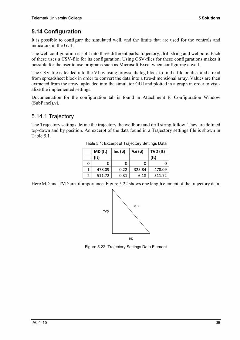
5.14.1 Trajectory

The Trajectory settings define the trajectory the wellbore and drill string follow. They are defined top-down and by position. An excerpt of the data found in a Trajectory settings file is shown in Table 5.1.

Table 5.1: Excerpt of Trajectory Settings Data

MD (ft) Inc (ø) Azi (ø) TVD (ft)

(ft) (ft)

0 0 0 0 0

1 478.09 0.22 325.84 478.09

2 511.72 0.31 6.18 511.72

Here MD and TVD are of importance. Figure 5.22 shows one length element of the trajectory data.

MD

TVD

HD

Figure 5.22: Trajectory Settings Data Element


IA6-1-15 39

Figure 5.23: Trajectory Plot

HD is needed in order to create the trajectory plot shown in Figure 5.23. Equation (5.5) shows how the values are related.

�� = �� − �� (5.5)

Each TVD and HD position is paired up and plotted as a point on the XY-graph of Figure 4.9. Each TVD and MD position is passed to the simulator core API when uploaded.

Documentation for the Trajectory settings tab is found in Attachment F: Trajectory Config (SubPanel).vi.


IA6-1-15 40

5.14.2 Drill String

The Drill String settings define the diameters and length sections of a drill string, and are defined bottom-up and by length elements. An excerpt of the data found in a drill string settings file is shown in Table 5.2.

Table 5.2: Excerpt of Drill String Settings Data

Component Section Length I.D. O.D.

(ft) (in) (in)

Bit 1.5 2.5 7.625

Rotary Steera-ble 29.3 2.5 7.625

MWD Tool 37 2.25 8.25

I.D. and O.D. are abbreviations for inner diameter and outer diameter, respectively. The raw sec-tion lengths and diameters are passed to the simulator core API. To create the plot, the length elements are cumulatively summed and prefixed with a 0-element, so that they become a positional array. The diameter elements are divided by 2 to become radius. Points are then created in an XY-plot and drawn lines between to create an image similar to the one seen in Figure 5.24. One of these is created for both the inner and outer diameters, to achieve the plot seen in Figure 4.10.

Ele

me

nt 0

Ele

me

nt 1

(R[0], P[0])

(R[0], P[1])

(R[1], P[1])

(R[1], P[2])(-R[1], P[2])

(-R[1], P[1])

(R[0], P[1])

(-R[0], P[0])

Figure 5.24: Drill String and Wellbore Plot

Documentation for the Drill String settings tab is found in Attachment F: Drillstring Config (SubPanel).vi.

5.14.3 Wellbore

The Wellbore settings define the well annulus by its lengths and diameters, and are defined top-down. An excerpt of a Trajectory settings file is shown in Table 5.3. The raw lengths and diameters are passed to the simulator core API, and the plot seen in Figure 4.11 is created the same way as the Trajectory plot, explained in Chapter 5.14.1.

Table 5.3: Excerpt of Wellbore Settings Data

Inner Diameter Length

(in) (ft)

10.75 9000

10 4830

9.5 2750


IA6-1-15 41

Documentation for the Trajectory settings tab is found in Attachment F: Wellbore Config (SubPanel).vi.

5.14.4 Limits

As some values are displayed multiple places in the GUI, several controls and indicators use the same inputs or outputs in the simulator core. To ensure that the limits always are the same for these controls and indicators, they all get their limit settings from the limits configuration. These con-figurations ensure that the limits always are the same for the same simulator core input or output. The inputs and outputs affected by these limits are the controls and indicators in the simulation and process window, the joysticks and the graphs.

Documentation for the Trajectory settings tab is found in Attachment F: GUI Limits Config (SubPanel).vi.

5.15 Trend

The GUI relies on time stamped plotting to display the history of different values. A chart would normally be sufficient for this task; however, a chart relies on synchronized threading, meaning that the chart must be in the same loop as the data it is plotting in order to keep track of the time stamps. In addition, the chart does not support different time intervals between plot data, this be-comes a problem when the GUI changes simulation speeds.

To work around this problem, a combination of a circular buffer and a graph is used. The circular buffer’s functionality is to store values in a buffer with a certain size. When a value is inserted into the buffer, the value is stored at the first empty space in the buffer as illustrated in Figure 5.25.

Figure 5.25: Insert Value into Buffer

If the buffer is full, new values are stored from the start of the buffer, overwriting old values in the process as illustrated in Figure 5.26.

Figure 5.26: Overwrite Value in Buffer


IA6-1-15 42

In the GUI, the circular buffer stores the sim time (Tn) with values for that given time in an array, in the same buffer slot as illustrated in Figure 5.27.

Figure 5.27: Array in Buffer

The values are read from the buffer and written into a graph with the sim times as the x-axis and the values along the y-axis. For every iteration, the graph is updated to match whatever is in the buffer.

Since the values are linked to specific sim time, the sample time of the graph’s loop is irrelevant for the time stamps in the graph. This makes it possible for the graph to have unsynchronized threading (can be in a different loop than the buffer). This also makes it possible to have different time intervals between plot data.

Documentation of the Circular Buffer is found in Attachment G: Circular Buffer.vi.

Telemark University College 6 Controller

IA6-1-15 43

6 CONTROLLER

Controlling DHP is one of the main challenges of oil drilling. Doing this autonomously provides the benefit of being able to drill in challenging environments, where the difference between frac-ture pressure and collapse pressure is small and conventional drilling falls short. Thus, having a well-designed controller is important in MPD, as it is crucial to ensure safe and economic drilling.

Kelda Drilling Controls is developing a robust model-based controller for pressure management, which is going to be compared to the PI controller designed in this project. It uses a DHP-estimator which estimates DHP using choke pressure, hydrostatic pressure and friction given by flow and drill string rotation [11]. This means that the DHP may be controlled by controlling choke pressure, which is an easier task than controlling DHP directly, due to the negligible time-delay from changes in choke position to measured choke pressure.

The goal of tuning this PI controller is to make it able to keep the choke pressure at a desired reference (set point), handle disturbances in flow and handle changes in set point. 10 – 12 bars is chosen as the operating range of the choke pressure set point, which is a common scenario. The choke pressure is controlled by changing the choke opening1. A smaller opening builds up pressure behind it. Maximum accepted deviation from set point ranges from 2.5 to 5 bars.

6.1 Pressure Model

The model for choke pressure is seen in Equation (6.1) [12].

�̇�(�) =

� ��(�) − ��2(��(�) − ��)

� ��(�)��

�

(6.1)

For the specific well that is being used to benchmark the controller, the values are seen in Table 6.1.

1 The choke opening will in reality have a maximum speed of movement. This dynamic is not implemented in the simulator core at the time of writing this report, thus the results seen in this chapter will not be realistic. Consequences of having an instantly-moving choke may be that the system’s gain margin becomes unrealistically high.


IA6-1-15 44

Table 6.1: Symbol List with Values

Symbol Description Value

�� Choke Pressure ��(�) Pa

� Mud Bulk Modulus 1 ∙ 109 Pa

�� Mud Flow into Choke ��(�) m3 s-1

�� Choke Valve Area 6.12 ∙ 10-5 m2

�� Atmospheric Pressure 105 Pa

� Mud Density 1500 kg m-3

�� Choke Opening 0 – 1 (See Table 6.2) -

�� Choke Signal 0 – 1 (See Table 6.2) -

� Mud Volume 250 m3

Table 6.2 shows the choke characteristics – the relationship between the choke signal (��) and the choke opening (��).

Table 6.2: Choke Characteristics

�� (��)

0.000 1.634 ∙ 10-6

0.2000 1.634 ∙ 10-6

0.3740 0.1159

0.4290 0.2403

1.000 1.000

6.2 Skogestad’s Method

A model based tuning method is chosen to tune the PI controller, more specifically Skogestad’s Method. It was chosen because of the option to change the desired speed of the system, making it possible to tune into not overshooting2 in the case of a step in reference. This is important for avoiding fracturing or collapsing a drilling well. It is based on the feedback system shown in Figure 6.1, and the controller described in Equation (6.2).

2 Overshooting is when the process value runs past the set point after a step in set point.


IA6-1-15 45

Cu

G

-

er y

Figure 6.1: Simplified Controller and Process Model

� =

�

�= �� 1 +

1

�� (6.2)

Here � is the controller and � is a linear process model, in this case the choke to choke pressure model. As seen in Equation (6.1), the pressure model is not linear, and a step response method of reducing the model is used to approximate linearity.

Skogestad’s Method is shown in the following equations [13]:

�� =

1

�

�

�� + � (6.3)

�� = ��, 4(�� + �)� (6.4)

� =

∆�

∆u (6.5)

Where

�� is the controller’s proportional gain

�� is the controller’s integral time

� is the process gain

� is the process time constant

� is the delay

�� is the desired system time constant

∆� is the difference in process value, in this case pressure

∆u is the difference in signal, in this case choke signal3

6.3 Step Response

To obtain � and �, it is necessary to perform a step in the choke signal.

3 Since the choke characteristic is nonlinear, the inverse of the choke signal will be used, effectively turning the choke signal into choke opening, such that the signal that is controlled is �� rather than ��.


IA6-1-15 46

Table 6.3: System Values for Step Response

Symbol Description Value

�� Mud Pump Flow 2000 L min-1

�� Back Pressure Pump Flow 0 L min-1

�� Choke Signal Start 55 %

�� Choke Signal End 45 %

Figure 6.2: Signal Step Response – u1 to u2

Table 6.4: Measured Values from Step Response

∆� -10 %

∆� 4 bar

� 11 s

� -0.4 bar %-1

Figure 6.2 shows how the choke pressure responds to the step with the values found in Table 6.3. Table 6.4 shows the measured response values.

Since the process gain (�) is negative, the controller must have direct action. This means that the controller gain (��) must be negative. In the GUI implementation however, �� is always positive, because the value is negated within the program code.


IA6-1-15 47

6.4 Controller Response

The controller response is tested with the values in Table 6.5. Three different values of �� are explored. The response is tested on changes in reference and different changes in flow (disturb-ances). The results are found in Attachment H: PI Controller without Feed Forward.

Table 6.5: Controller Response Test Values

�� 10 bar

�� 12 bar

�� 2000 L min-1

�� 1000 L min-1

�� 2500 L min-1

�� 4000 L min-1

A relatively low �� is chosen in the first case. See Table 6.6 for PI parameters. The results show that after the set point change, the pressure overshoots by about 2 bars before quickly falling in line with the set point. All disturbances are quickly compensated for, and the deviations from set point are less than 1 bar.

Table 6.6: Low τc PI Parameters

�� 2 s

�� -13.8 % bar-1

�� 8 s

Table 6.7 contains the PI parameters which is used in the case of medium ��. The results show that the system responds quickly to changes in set point, without overshooting. Disturbances are slowly compensated for, with the pressure deviating little more than 1 bar from the set point.

Table 6.7: Medium τc PI Parameters

�� 5 s

�� -5.5 % bar-1

�� 11 s

Table 6.8 contains the PI parameters used in the case of a high ��. After a change in set point, the pressure slowly approaches the reference with no overshoot. Disturbances cause the pressure to deviate by more than 2 bars before slowly approaching the set point.


IA6-1-15 48

Table 6.8: High τc PI Parameters

�� 15 s

�� -1.8 % bar-1

�� 11 s

6.5 Feed Forward

Since the case of low �� in some cases causes overshoots, and the case of high �� gives large deviations after flow disturbance, medium �� is chosen for selection of PI parameters. To reduce deviations caused by disturbances and to keep the pressure at the set point in case of a power loss4, feed forward control is used.

The model for the choke pressure is given by Equation (6.1). This is used to obtain the feed forward signal, by the method found in [14]. The feed forward signal is found in Equation (6.6).

��,��(�) =

√2

2

��(�)

��,��(�) − ��

�

(6.6)

�� is the sum of the back pressure pump flow (��) and the mud pump flow (��). ��’s effect

on the pressure comes instantaneously, but �� takes a while to reach the choke. Thus, it is rea-

sonable to delay the effect of that flow with that time (�). The time-delay is found in Equation (6.7).

� =

2��ℎ

�� (6.7)

It has also been found that the flow through the choke caused by �� is approximately a first-order

process, where the time constant, ��, has been found by experiment to be around 20 s in the desired range of operation. Thus, the mud pump flow used for calculating the feed forward contri-bution is described by Equation (6.8).

��,��

��=

��

�� + 1 (6.8)

This gives (6.9) for the feed forward contribution.

4 A power loss causes the mud pump flow to drop quickly to 0.


IA6-1-15 49

��,��(�) =

√2

2��,��(�) + ��(�)

��,��(�) − ��

�

(6.9)

6.5.1 Tests

The controller with feed forward will be tested by using the medium �� parameters, and the same scenarios found in Chapter 6.4. In addition a test emulating a power loss will be used, seen in Table 6.9. The results are found in Attachment H: PI Controller with Feed Forward.

Table 6.9: Power Loss Flow Value

�� 0 L min-1

The results show that after the change in set point, the pressure overshoots by 1 bar before quickly returning to the reference. The disturbances show that the pressure deviates by less than 1 bar before quickly returning to the set point. After the power loss, the pressure deviates by up to 1.5 bars before stabilizing at 1 bar below the set point.

6.6 Gain Scheduling

Since the choke pressure is a nonlinear process, a controller may only perform well around the parameters that were used to tune it. Figure 6.3 shows the PI controller tuned to the medium set-tings, but at a set point step from 40 to 45 bars, which may also be a common scenario. It is clearly visible that the system is initially unstable, which is undesirable.

Figure 6.3: From 40 to 45 bars

A solution for this is to use gain scheduling with the choke pressure set point as the controlling parameter [15]. This can be done by tuning the controller at several different parameter settings, and use interpolated values. It is also possible to calculate the PI parameters continuously by com-bining the pressure model from Equation (6.1) and Skogestad’s method. Here the former will be investigated.


IA6-1-15 50

The PI parameters are found by the same method as in Chapter 6.4, but by adjusting the choke opening so that we get four operating ranges from about 10 to 50 bars. The medium �� setting will be used (5 s). The mud pump flow will remain at 2000 L min-1. Table 6.10 shows the values found.

Table 6.10: Gain Scheduling PI Parameters

��,��

[bar]

��

[%]

��

[%]

�

[s]

�

[bar %-1]

��

[% bar-1]

��

[s]

11 50 45 11 -0.25 -8.8 11

22 35 30 27 -1.4 -3.9 20

37 28 25 36 -2.6 -2.8 20

48 24 22 50 -3.9 -2.6 20

6.7 Results

The complete controller including gain scheduling and feed forward control will be tested as shown in Table 6.11 and Table 6.12. The results are found in Attachment H: Gain Scheduled PI Controller with Feed Forward.

Table 6.11: Tests

Test Set Point Mud Pump Flow

1 �� to ��

2 �� to ��

3 �� to ��

4 �� to ��

5 �� to ��

6 �� to ��

7 �� to ��

8 �� to ��

9 �� to ��

10 �� to ��


IA6-1-15 51

Table 6.12: Test Values

�� 10 bar

�� 12 bar

�� 40 bar

�� 45 bar

�� 2000 L min-1

�� 1000 L min-1

�� 2500 L min-1

�� 4000 L min-1

�� 0 L min-1

The results show that at the lower bound set points, the measurements are nearly identical to those of Chapter 6.5. The tests at the higher bound set points shows that the system is stable, and pro-duces results that are within the accepted limits for all disturbances, including the power loss sce-nario, where the pressure stabilizes at 3 bars below the set point. The gain scheduled PI controller with the parameters from Table 6.10, together with the feed forward function from Equation (6.9) gives a controller which performs within the acceptable limits.

Telemark University College 7 Discussion

IA6-1-15 52

7 DISCUSSION

7.1 GUI

Having developed “Straume Hydraulic Simulator” in LabVIEW has enabled rapid development of the application. It requires that the user has LabVIEW Run-Time Engine installed and this de-pendency suggests that the application is not lightweight. It was created with a strong focus on flexibility of customization, and having multiple programmers working on the GUI simultane-ously. In addition, large amounts of elements used in the GUI were custom designed. This made the GUI appear less like a LabVIEW-produced software, as was desired by Kelda.

The GUI was designed to be easy to understand. This was managed by using common rig termi-nology and plots, as well as a minimalistic design where the user only receives relevant infor-mation.

Key values are logged in the different graphs, and the graphs have an adjustable time-axis in order to display the wanted history. This tool allows for demonstration of drilling behavior. In addition, the GUI has the ability to run pre-recorded inputs, known as scenarios, by reading MAT-files.

The PFD described in Chapter 4.2 gives the user a visual interaction with the drilling process, and gives an overview of the process in its entirety.

7.2 Controller

The choke dynamics of the system are neglected in the simulation model, thus the simulated results found in Chapter 6 are better than in a real-world scenario, and must be critically reviewed. The consequences are that the choke pressure dynamics becomes a first order process, rather than a higher order process (which would be closer to the real-world dynamics). This means that the phase difference will not exceed 90°, thus the system will have an infinite gain margin [16].

The results are conditional upon the ability to map the characteristics of the choke valve. This is possible using the knowledge of how flow, pressure and the choke opening relates, by testing it live at different input signals. An approximation method may be used to fit a function to the valve characteristics, e.g. B-spline approximation [17].

The results from Chapter 6 show that a conventional PI controller alone gives a process that either reacts slowly to disturbances or is unstable in operating ranges outside the one used to tune the controller. Adding feed forward control protects against disturbances, and using a gain scheduled PI controller gives stability in a larger operating range.

7.3 Workflow

Using Scrum, TDD, version control and automatic documentation has been central to the devel-opment of the GUI. It has ensured productivity, traceability and structure throughout the develop-ment process. Having regular sprint meetings (stand-ups, planning, reviews) has enabled Kelda and the project group to work closely together. It has provided Kelda with the opportunity for frequent input regarding the GUI features, and the project group with the opportunity for assistance when needed.

Telemark University College 8 Conclusion

IA6-1-15 53

8 CONCLUSION

The task of developing a GUI and controller for Kelda’s oil drilling simulator was approached with focus on user experience and robustness. The development has followed the Scrum project method, and used version control tools and automatic documentation. TDD has been used to a limited degree, on stand-alone mathematical functions only.

The GUI is developed to access all the simulator core’s features while being easy to use. It has the ability to be configured to different wells using CSV-files defining wellbore, trajectory and drill string data. It also has the ability to save new configuration data. Other features include status bar, running the simulation faster than real-time, being able to change choke pressure controller, visu-alizing mud changes, and being controlled by joysticks and pre-recorded inputs.

By analyzing both the given pressure model and step responses, a PI controller that provides sat-isfactory results has been developed to control choke pressure. It utilizes feed forward control and gain scheduling to handle disturbances and nonlinearity. The controller makes the system stable, and satisfies the deviation requirements of 2.5-5 bars after rig pump disturbance, power loss and changes in set point. It will be a reference for Kelda’s more advanced model-based controller.

The simulator core and GUI will continue to be work-in-progress, and there are several concrete features suggested for future development:

Bump-less switching of controllers

Go to steady-state after startup and configuration

Group indicators and controls by function

Establish interface between BOP and Mud Visualization and Simulator Core

Support several screen resolutions

Support dynamic scaling

Implement Kelda’s DHP controller

Add mud and temperature configuration

Add the possibility to record simulations

Add the possibility to start from a point in a recorded simulation

Filter set point value to ensure smooth transitions

Add ability to implement new controllers without changing code

It is recommended that the GUI development follows the simulator core’s development cycle, thus always staying up to date.

Telemark University College References

IA6-1-15 54

REFERENCES

[1] Halliburton, “Asphaltene Control”, [Online]. Available: http://www.halliburton.com/en-US/ps/multi-chem/pipeline-integrity-challenges/Asphaltene-Tendencies.page . [Acquired: 5 May 2015].

[2] Naoki Schwartz and Harry R. Weber, “Bubble of methane triggered rig blast,” Southern California Public Radio, May 08 2010. [Online]. Available: http://www.scpr.org/news/2010/05/08/14902/bubble-methane-triggered-rig-blast/. [Acquired 13 March 2015].

[3] National Oilwell Varco, “Blowout Preventers” [Online]. Available: https://www.nov.com/Segments/Rig_Systems/Land/Drilling_Pressure_Control/Blow-out_Preventers.aspx . [Acquired 08 April 2015].

[4] ContiTech, “Instructions for the use of choke and kill lines” [Online]. Available: http://www.contitech-rubber.hu/pages/service/documents/downloads/hose_han-dling_doc_TKO_AS2.pdf . [Acquired 13 May 2015].

[5] J. Y. Fiset, “Human-Machine Interface Design for Process Control Applications” [Online]. Available: https://books.google.no/books?id=NE_TEJBmwi8C&printsec=frontcover&hl=no&source=gbs_ge_summary_r#v=onepage&q&f=false . [Acquired: 10 February 2015].

[6] K. Schwaber and J. Sutherland. (2013). “The Scrum Guide”. Available: http://www.scrumguides.org/scrum-guide.html. [Acquired: 8 May 2015].

[7] J. Stepka. (2011). “Bitbucket now rocks Git”. Available: http://blog.bitbucket.org/2011/10/03/bitbucket-now-rocks-git/. [Acquired: 8 May 2015].

[8] R. Osherove, “The Art of Unit Testing”. Shelter Island: Manning, 2014.

[9] Halliburton, “Mud Pulse Telemetry System” [Online]: http://www.halliburton.com/en-US/ps/sperry/drilling/telemetry/mud-pulse-systems.page. [Acquired 13 May 2015].

[10] D. J. Cooper. (2008). “Practical Process Control” [E-book]. Available: http://www.controlguru.com/.

[11] J.M. Godhavn et al., “Drilling seeking automatic control solutions,” in Preprints of the 18th IFAC World Congress, Milano (Italy), 2011.

[12] G.O. Kaasa et al., “Simplified Hydraulics Model Used for Intelligent Estimation of Downhole Pressure for a Managed-Pressure-Drilling Control System,” SPE Drilling & Completion, vol. 27, pp. 127-138, 2012.

[13] S. Skogestad, “Simple analytic rules for model reduction and PID controller tuning,” Journal of Process Control, vol. 13, 2003.

[14] F. Haugen, “Reguleringsteknikk”. Trondheim: Akademika Forlag, 2012.

[15] E. Jahanshahi and S. Skogestad, “Comparison between nonlinear model-based controllers and gain-scheduling Internal Model Control based on identified model,” in 52nd IEEE Conference on Decision and Control, Florence (Italy), 2013.

[16] J. G. Balchen, et al. “Frekvensanalyse” in Reguleringsteknikk, 2nd ed. Trondheim, Norway: ITK, 1999.

[17] P. Robertson, “B-spline approximations in an optimization framework,” M.S. thesis, ITK, NTNU, Trondheim, Norway, 2013.

Telemark University College Attachments

IA6-1-15 55

ATTACHMENTS

All attachments are found on the attached CD-ROM.

Attachment A Bachelor Project

Attachment B Sprint Plan

Attachment C Sprint Report

Attachment D Straume C-API User Manual

Attachment E Automatic Documentation Generator

Attachment F Straume Hydraulic Simulator – Subpanels

Attachment G Straume Hydraulic Simulator – SubVIs

Attachment H Controller Measurements and Results

telemark university college - halvorsen.blog · telemark university college foreword ia6-1-15 2...

Documents