teknisk rapport - sintef · 2014. 11. 17. · cycle assessment (lca) perspective in planning of...
TRANSCRIPT


3
12X277 TR A6558
TABLE OF CONTENTS Page
1 INTRODUCTION ...............................................................................................................5
2 PRINCIPLES FOR THE PLANNING METHODOLOGY................................................8
3 LOCAL ENERGY PLANNING FLOWCHART ...............................................................9 3.1 ENERGY STUDY PLANNING .........................................................................10 3.2 ENERGY SERVICES – DEMAND AND PROGNOSIS ..................................14 3.3 ALTERNATIVES DEVELOPMENT – OPTION SEARCH .............................16 3.4 IMPACT ASSESSMENT ...................................................................................17 3.5 IMPACT EVALUATION...................................................................................22 3.6 OPTIMISATION – SENSITIVITY ANALYSES ..............................................23 3.7 CORPORATE ECONOMICS – RISK EVALUATION.....................................24 3.8 CONCESSION PROCESS – EXTERNAL ECONOMICAL SUPPORT
PROCESS(ES) ....................................................................................................24 3.9 FINAL DECISION – IMPLEMENTATION OF PROJECT..............................26
4 PLANNING TOOLS.........................................................................................................27 4.1 OBJECTIVE OF ENERGY PLANNING TOOLBOX.......................................27 4.2 USERS.................................................................................................................28 4.3 THE CONTENT OF THE ENERGY SYSTEM PLANNING TOOLBOX .......28 4.4 THE ORGANIZATION OF THE ENERGY SYSTEM PLANNING
TOOLBOX..........................................................................................................29 4.5 SUMMARY ........................................................................................................33
5 REFERENCES ..................................................................................................................34
APPENDIX 1: DECISION MAKERS, STAKEHOLDERS AND STAKES...............................37
APPENDIX 2: LOAD MODELLING ..........................................................................................45
APPENDIX 3: MULTI-CRITERIA DECISION AID FOR ENERGY PLANNING...................57
APPENDIX 4: UNCERTAINTY..................................................................................................73
APPENDIX 5: CASE STUDIES ..................................................................................................81


5
12X277 TR A6558
1 INTRODUCTION This report represents part II of the results from the R&D project ‘SEDS – Sustainable energy distribution systems: Planning methods and models’ for the project period 2002 – 2007. The main partners within SEDS have been:
• Department of Electric Power Engineering, Norwegian University of Science and Technology (NTNU)
• Department. of Energy and Process Engineering, NTNU • Department of Energy Systems, SINTEF Energy Research • Department of Energy Processes, SINTEF Energy Research
The project has been funded by the Research Council of Norway, StatoilHydro, Statkraft alliance (Statkraft SF, Trondheim Energi, BKK), Lyse Energi and Hafslund Nett, while Norwegian Water Resources and Energy Directorate (NVE) has been a co-operating partner. Our international partners have been University of Porto and INESC Porto in Portugal, Helsinki University of Technology and VTT in Finland as well as Argonne National Laboratory in USA and Swiss Federal Institute of Technology (ETH) in Switzerland. The main objectives of the SEDS project, as stated in the original project plan have been the two following:
1. Develop methods and models that allow several energy sources and carriers to be optimally integrated with the existing electric power system. Particular emphasis is placed on distribution systems and integration of distributed energy sources, from a technical, economic and environmental point of view.
2. Develop a scientific knowledge base built on a consistent framework of terminology and concepts for mixed energy systems, in the field of planning methods and models. This will be a cornerstone for the curriculum ‘Energy and environment’ at NTNU.
Mixed energy distribution systems are illustrated in Figure 1. A mixed energy distribution system means (in this context) a local energy system with different energy carriers (electricity, district heating, natural gas, hydrogen) and a mix of distributed energy sources and end-uses.

6
Figure 1 A mixed energy distribution system.
Thus, it is the scientific based methods and models for planning mixed energy distribution systems which are focused in the SEDS project. The term sustainable in the project name should be interpreted in this context. Sustainability relates to all aspects of the recommended planning objective: Economy, quality, security, safety, reputation, contractual aspects and environment. Hence, different energy distribution system alternatives should be characterized with respect to all these objectives, and the planning process should clearly quantify and make these parameters visible and understandable to decision makers and stakeholders, enabling the decision makers to choose sustainable system solutions. The first objective has been realized through PhD-studies within the following three areas:
• Load and customer modelling of combined end-use (heating, cooling, electricity) • Quality and reliability of supply in mixed energy systems • Multiple criteria decision methods for planning of mixed energy distribution systems
In addition an initial study has been performed focusing on environmental impacts using a life cycle assessment (LCA) perspective in planning of local energy systems. The project has also funded a post doctoral fellowship in multi-criteria decision aid and risk based methodology, and a tutorial given by our partners at University of Porto about risk analysis and multi-criteria decision making. The second objective has been grouped in two parts:
• Development of a consistent planning framework for mixed energy distribution systems (terminology, concepts, socio-economic principles, general methodology etc)
• Development of a software toolbox environment (web-site) for decision support, visualization and demonstration of methodologies and technologies
12X277 TR A6558

7
12X277 TR A6558
For this part SEDS has co-operated with the eTransport project at SINTEF Energy Research 1, where a new tool for planning of energy systems is developed, considering several energy carriers and technologies for transmission and conversion. The main products from the SEDS project are:
• Technical reports: “Planning of sustainable energy distribution systems” in four parts [1] [20] [21]
• Web-site for energy planning methods and tools [2] • Three PhD candidates [21] • Publications in international journals and conference papers [21] • Presentations at workshops and seminars [21] • Numerous student project reports and Master theses [21]
The SEDS results constitute a scientific knowledge base for the curriculum Energy and environment at NTNU as well as for energy distribution companies, energy authorities like NVE and governmental agencies like Enova and other stakeholders interested in local energy planning.
1 eTransport-report: Energy 32 (2007), Elsevier

8
12X277 TR A6558
2 PRINCIPLES FOR THE PLANNING METHODOLOGY The initial problem identification and formulation in the SEDS project related to planning of mixed energy distribution systems provides an outline of the main elements in the planning process [1]. These comprise the objectives, main phases, tasks/ steps and analyses, summarized in the following to serve as an introduction to the planning methodology description. The main objectives for the planning process are as follows:
• To cover supply duties with acceptable quality of supply and to contribute to effective energy markets
• Design infrastructure and mix of energy sources and carriers to minimum cost and acceptable environmental impact
• Optimise interplay between the infrastructure and demand side management This report gives a recommended flowchart for the local energy planning process with a short description of the different planning elements.
9
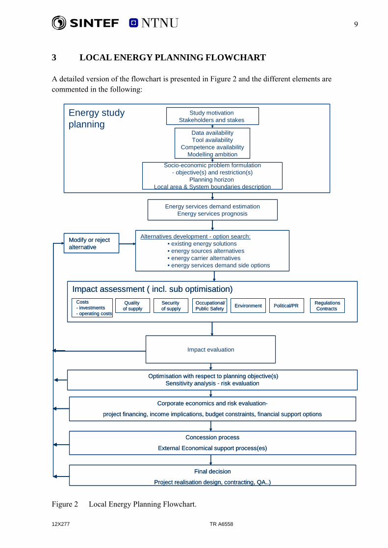
3 LOCAL ENERGY PLANNING FLOWCHART A detailed version of the flowchart is presented in Figure 2 and the different elements are commented in the following:
Energy services demand estimationEnergy services prognosis
Alternatives development - option search:• existing energy solutions • energy sources alternatives• energy carrier alternatives• energy services demand side options
Costs- investments- operating costs
Quality of supply
Occupational/Public Safety Environment Political/PR Security
of supplyRegulationsContracts
Modify or reject alternative
Impact assessment ( incl. sub optimisation)
Optimisation with respect to planning objective(s)Sensitivity analysis - risk evaluation
Corporate economics and risk evaluation-
project financing, income implications, budget constraints, financial support options
Concession process
External Economical support process(es)
Final decision
Project realisation design, contracting, QA..)
Impact evaluation
Study motivation Stakeholders and stakes
Data availabilityTool availability
Competence availabilityModelling ambition
Socio-economic problem formulation- objective(s) and restriction(s)
Planning horizon Local area & System boundaries description
Energy studyplanning
Figure 2 Local Energy Planning Flowchart.
12X277 TR A6558
10
12X277 TR A6558
3.1 ENERGY STUDY PLANNING 3.1.1 Study motivation – Problem formulation As in any problem solving, problem formulation is a key success factor. To identify what motivates the study is hence vital in order to define the problem correctly and consistently. If the problem is the gap between the “present situation” and the “desired situation”: “problem” = “desired situation” - “present situation” a local energy planning project might be motivated by the notion of an existing gap. The larger the gap is expected to be, the more important is it to address the problem. Anyhow, it is essential to perform a rough fact finding process as a gross estimate of the gap. This might be helpful to motivate resource allocation and to design the study properly. Who are the stakeholders affected and what are their preferences is an aspect to be considered in a local energy planning study. One of the main criteria to be fulfilled in a socio-economic analysis is to consider all relevant impacts for all stakeholders affected thus qualifying this sub process. An illustration of main stakeholders and examples of main objectives is given in Table 1.
Table 1 Energy Systems Stakeholders and Objectives. Examples.
Stakeholder Objectives (examples)
Local energy system operator(s)
Good performance - good service - good reputation - fair/high income
Local energy system owner(s)
Rate of return on assets - new spin-off business areas - regional industrial development. Good reputation
Energy regulators - NVE Maximum efficiency - incentives for quality of supply
Directorate for Civil Protection and Emergency Planning – DSB
Promote measures which prevent accidents, crises and other undesired incidents
Norwegian Pollution Control Authority - SFT
Promote measures to combat emissions
Local energy customers Low tariffs - 100% reliability – low cost installations- safe installations
Governmental agency - Enova
Environmentally sound and rational use and production of energy. To stimulate market actors and mechanisms to achieve national energy policy goals.
Local and regional governments
Regional industrial development. Development of residential areas. Low tariffs. Limited environmental impact. Implementing national goals and policies.
Ministry of Petroleum and Energy
The principal responsibility of the Ministry of Petroleum and Energy is to achieve a coordinated and integrated energy policy.
Ministry of the Environment The Ministry of the Environment has a particular responsibility for carrying out the environmental policies of the Government and in this context also for the planning part of The Planning and Building Act
Ministry of Local Government and Regional Development
In this context the Ministry is responsible for the Norwegian housing policy, district and regional development and also for the building part of The Planning and Building Act
Contractors, investors Maximise profit, maximise return on investments
11
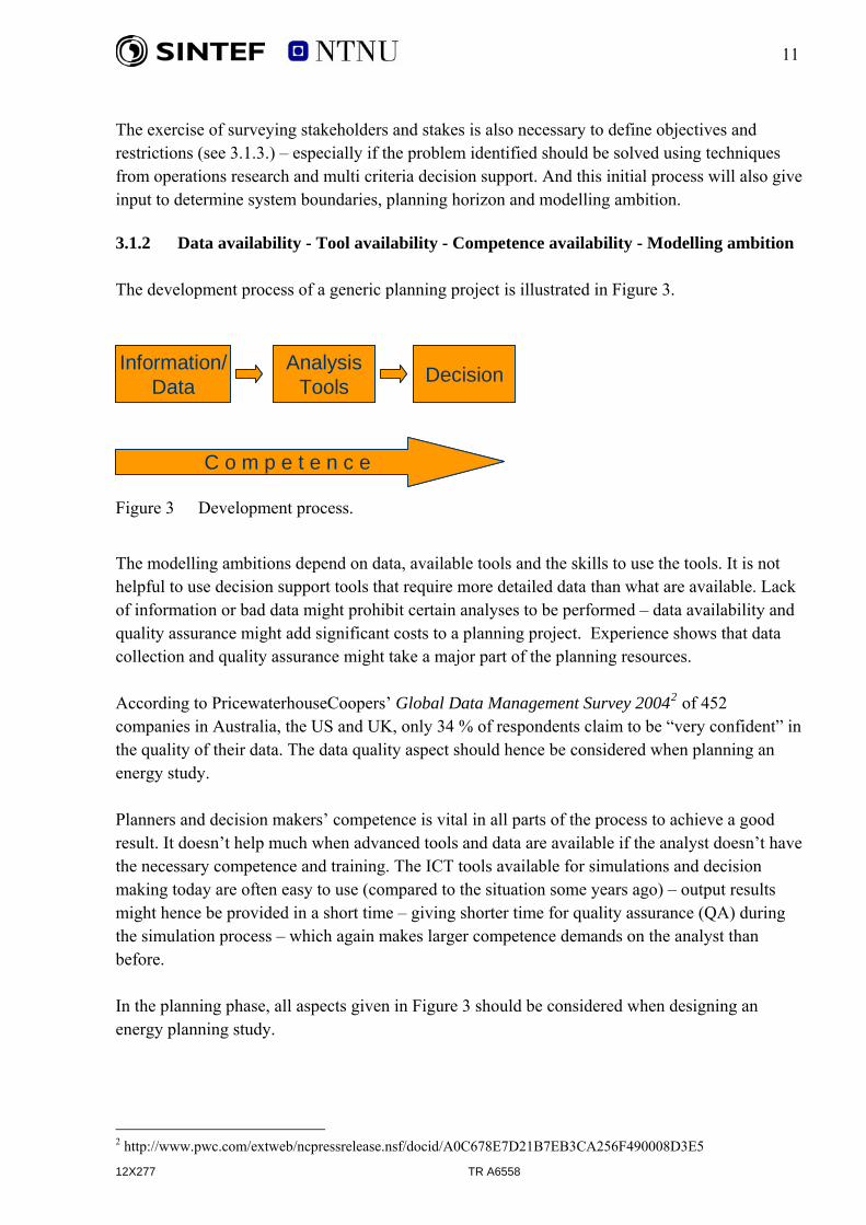
The exercise of surveying stakeholders and stakes is also necessary to define objectives and restrictions (see 3.1.3.) – especially if the problem identified should be solved using techniques from operations research and multi criteria decision support. And this initial process will also give input to determine system boundaries, planning horizon and modelling ambition. 3.1.2 Data availability - Tool availability - Competence availability - Modelling ambition The development process of a generic planning project is illustrated in Figure 3. Information/
Data DecisionAnalysisTools
Information/Data DecisionAnalysis
Tools
C o m p e t e n c eC o m p e t e n c e
nergy study.
have
ng lation process – which again makes larger competence demands on the analyst than
efore.
l aspects given in Figure 3 should be considered when designing an energy planning study.
Figure 3 Development process.
The modelling ambitions depend on data, available tools and the skills to use the tools. It is not helpful to use decision support tools that require more detailed data than what are available. Lack of information or bad data might prohibit certain analyses to be performed – data availability and quality assurance might add significant costs to a planning project. Experience shows that data collection and quality assurance might take a major part of the planning resources. According to PricewaterhouseCoopers’ Global Data Management Survey 20042 of 452 companies in Australia, the US and UK, only 34 % of respondents claim to be “very confident” in the quality of their data. The data quality aspect should hence be considered when planning an e Planners and decision makers’ competence is vital in all parts of the process to achieve a good result. It doesn’t help much when advanced tools and data are available if the analyst doesn’t the necessary competence and training. The ICT tools available for simulations and decision making today are often easy to use (compared to the situation some years ago) – output results might hence be provided in a short time – giving shorter time for quality assurance (QA) durithe simub In the planning phase, al
2 http://www.pwc.com/extweb/ncpressrelease.nsf/docid/A0C678E7D21B7EB3CA256F490008D3E5
12X277 TR A6558

12
12X277 TR A6558
3.1.3 Socio-economic problem formulation - Planning horizon -System Boundaries 3.1.3.1 Problem formulation Based on the previous sub processes, the next step is more firmly to make a socio-economic problem formulation. The principles are described in [1]. In a decision making process, decision criteria need to be formulated as a tool to choose among alternatives. An objective function is a mathematical formulation of such a criterion and is hence a way of formalizing the socio-economic problem formulation. One definition of the term objective function is: A function associated with an optimization problem which determines how good a solution is. The overall objective as stated in the Norwegian Energy Act is to ensure that generation, conversion, transmission, trading and distribution of energy are rationally carried out for the benefit of society, having regard to the public and private interests affected. This means that decision makers should have an holistic approach, implying that all costs and impacts related to the energy system for all stakeholders should be considered, not only those being part of the corporate economics. This objective can be met by applying socio-economic planning principles and analysis (see [1]). 3.1.3.2 Planning horizon The energy system assets usually have long expected technical lifetimes, typically 20 - 70 years. The planning horizon should hence be equally long to assess the future effect of present decisions over the life cycle of the components. Due to uncertainties like energy demand development, new technologies, cost development etc, a reasonable compromise is a planning horizon of 10 - 30 years depending on the project and its uncertainties. Local energy plans are not developed once and for all, but need to be revised due to changes in planning premises. A proposed action (investment) late in the period of analysis is expected to be revised (and changed) many times before the final decision of putting it into operation. The interest rate used to calculate net present values contributes to decide the weight of future costs in the objective used. In net present value calculations with high interest rates, the cost contribution from years late in the period of analysis might be small and hence have limited influence on decisions. 3.1.3.3 System boundaries As the overall energy system is very large, it is often necessary to limit the planning problem to a manageable size as planning resources (money and time) are limited. An important motivation for problem size reduction and hence model reduction, is to reduce data volume and to improve data

13
quality as discussed previously. Result interpretation might also be difficult when the models are very large. It is hence essential that the planning problem formulation and delimitation is carefully considered when the actual planning process is initiated. To reduce model size, system decomposition is a well known technique. Figure 4 illustrates the principle.
End Use
A B
Main energysystem
Local energysystem
Overall energysystem
Decomposition
Transmission DistributionMainenergysource
Local energysource
End Use
A B
Main energysystem
Local energysystem
Overall energysystem
Decomposition
Transmission DistributionMainenergysource
Local energysource
Figure 4 Planning problem decomposition – model reduction.
The overall energy system is divided into two subsystems [1]:
• The main system – i.e. the system level feeding the local energy system • The local energy system – i.e. the planning area - the system where actions are considered
The main energy system is not represented in any detail in the study, but the relevant planning signals from the main system to the local distribution system should be considered at the interface between the two systems in point A. The local distribution system is modelled to the level of detail that the study requires. To go into great modelling detail might be costly in terms of data collection and data quality assurance, while the use of too simplified and too aggregated models might give misleading conclusions. The end use is often represented by load equivalents (energy, power), load characteristics (type of load), energy outage/interruption costs etc. at point B. Often geography is a factor when limiting the planning area. System boundaries applied to energy systems are further discussed in [1].
12X277 TR A6558

14
12X277 TR A6558
3.2 ENERGY SERVICES – DEMAND AND PROGNOSIS The most fundamental task in a local energy planning study is to estimate present and future demand for energy services. The basic energy services are here defined to comprise:
• Light • Mechanical work • Heating (space heating, cooking, hot water..) • Cooling (air condition, refrigeration..) • Electronics (PC, TV, stereo…)
The metrics used for quantitative specifications of the energy services might be in terms of annual energy (J, Wh), power/peak power (J/s, W), load duration curves, annual, seasonal, daily variations etc. The different services should also be characterised with respect to whether the services can be performed by different energy sources or not. As an example space heating might be supported by several energy technologies – alone or in combination. For electronics, electricity is the only upstream technology that can be used. (But electricity can be generated from a variety of primary energy sources.) Local energy systems as illustrated in Figure 4 typically cover the parts of the energy system from a bulk supply point to aggregated load points representing different end-uses. The SEDS project focuses on irreversible energy distribution system infrastructure investments, i.e. pipes or cables for distribution of district heating, gas or electricity. An illustration is given in Figure 5. The figure shows cables for medium voltage electricity distribution and pipes for district heating and the aggregated load points (power and heat substations). In order to optimise energy supply infrastructure investments forecasting of spatial distributed energy usage is essential. The energy planner has to ask: What kind of energy is needed where and when? Can locally available energy sources contribute to cover the demand? The main challenge is to decide which energy carrier should be developed to which areas and what should be the capacities. Both the forecasted peak demand and the expected annual energy consumption and load profiles are important parameters in the design of the energy system.

15
Figure 5 Example of energy distribution infrastructures.
Load models are cornerstones for estimation and forecasting energy and power demand for different purposes. Load modelling can then be defined as aggregation of spatial, individual energy demand specified in time. In practice this is done by establishing representative load profiles for defined customer categories with similar demand. The different purposes normally require different emphasis on detailing level. In order to analyse the future energy demand in a specific area the customers need to be categorised in groups for which customers have similar demand profiles by day, by week and by season. The first approach is to divide customers in sectors like private households, public service, agriculture and industry. It is however obvious that a more detailed categorisation is needed since not only total consumption but also consumption specified on end-use and possible energy carrier need to be addressed. Some factors affect the total energy consumption while other factors will mainly influence the portion of each energy carrier. How these uncertainties have been evaluated should be documented during the energy planning process:
12X277 TR A6558

16
12X277 TR A6558
Factors affecting total energy demand
• Temperature/climate (heating/cooling) • Area heated and insulation (households/buildings) • Economic cycles, trading conditions (industry) • Technological development (possible peak shaving equipment) • Attitude of energy users (price sensitivities)
Factors affecting total energy demand for specific energy carrier
• Price and expected price forecast (incl. tax and duties/subsidies) o Availability/transport costs o Political decision
• Installed equipment (flexibility) • Dimensioning of infrastructure (technical losses) • Users’ preferences/user friendliness • Mutual dependencies between energy carriers
3.3 ALTERNATIVES DEVELOPMENT – OPTION SEARCH Given the identified local energy planning problem with its system boundaries, many alternatives might be established for the energy system development. An alternative can be defined as the description of a possibility (an option) that is relevant for the choice between mutually exclusive possibilities. An alternative can be characterized by a set of parameters:
• Energy sources • Energy carriers • Energy demand side options • Geographical location of sources, carriers, loads e.g. coordinates, routes… • Topology i.e. how the assets are connected • Redundancy • Dimensions i.e. rating of assets (sources, carriers...)
The existing energy supply solution is often the reference alternative which others are evaluated against. In some cases the existing solution is not an option. As an example when a new industrial plant is to be connected to the local energy supply area, the existing solution normally has to be modified leaving it out as an option. As indicated in the flowchart by the “modify or reject alternative” box, the number of alternatives in a given project is dynamic. All alternatives are not known initially. Results from simulations in the impact assessment sub process will create new ideas and information that might generate new alternatives.

17
3.4 IMPACT ASSESSMENT To assess the performance of different alternatives, impact evaluations need to be carried out. As decisions are related to future performance of the energy system, simulation tools are often used to establish the performance indicators required. Annual operating cost is one example of an economical performance indicator. CENS (Cost of Energy Not Supplied) is an example of a quality of supply performance indicator for electricity supply. “Expected number of days between accidents” is a safety performance indicator. Primary energy use is an energy efficiency indicator and annual CO2 and NOX emissions are environmental performance indicators. (Environmental indicators should cover both local and global effects.) The impact assessment is afforded by a chosen set of simulated performance indicators and should be linked to the stakes important for the stakeholders involved. In the flowchart the impact assessment is classified in 7 main groups indicating that decision makers will evaluate alternatives along different axes. The classification is especially relevant if different criteria are to be weighted in a multi criteria approach. Even if several impacts might be estimated in monetary terms, they might be weighted differently – an investment cost of 1 mill. NOK is not equivalent to an expected outage cost of 1 mill. NOK. As the main task of the overall process is to rank the different alternatives in order to choose among the better ones, it is crucial that the alternatives are treated in a consistent way so that comparison (ranking) is relevant. This aspect is indicated in the flowchart by the proposed “sub optimisation” to allow for maximum performance for each alternative. The aspect is further illustrated in Figure 6, where two alternatives are to be compared in terms of the operating costs.
Pipe diameter
Ope
ratin
g co
sts
Alternative A
Alternative B
Aopt
Bopt
A1
B1
Pipe diameter
Ope
ratin
g co
sts
Alternative A
Alternative B
Aopt
Bopt
A1
B1
Figure 6 Comparison of two alternatives.
From the figure it can be seen that alternative A has the largest inherent potential in terms of minimizing the operating costs if the diameter is chosen carefully (each alternative is optimized separately). Alternative A is more sensitive than alternative B with respect to this parameter. If the
12X277 TR A6558
18
12X277 TR A6558
analyst doesn’t have performed the necessary individual/separate optimization, the operating costs used in further economical analyses could be A1 and B1 – giving a preference for alternative B which is quite misleading. The comparable operating costs that should be used in the further analysis are Aopt and Bopt. The different impact categories in the flowchart are briefly discussed in the following. 3.4.1 Costs (economy) One of the main objectives in socio-economic local energy planning is to minimize all relevant costs while meeting relevant restrictions. As an example the Norwegian energy regulator (NVE) has included the following cost elements in the planning requirements for electrical energy networks [12]:
• Investment costs- including reinvestment and renewal costs • Operating and maintenance costs- including utility repair and damage costs • Cost of electrical losses • Customer outage costs - costs of energy not supplied (CENS) • Congestion costs
The same principal cost elements could be included in any local energy planning problem though the weight and the relevance might vary from project to project. 3.4.2 Quality of supply Quality of supply is an essential aspect of energy supply of concern for most stakeholders especially energy supply customers. What is quality of supply? According to The Council of European Energy Regulators (CEER) working group on quality of electricity supply, quality of supply in electrical supply systems may be divided into three main categories [11].
• Commercial quality • Continuity of supply (reliability) • Voltage quality
Commercial quality Concerns the quality of relationships between a supplier and the individual user. Commercial quality covers many aspects of the relationship, for example the maximum time to provide supply, metering, reading and billing, information, telephone enquiry responses, management of customers’ complaints, emergency services and others.

19
12X277 TR A6558
Continuity of supply (reliability) Is characterized by the number and duration of interruptions. Several indicators may be used to characterize the impact on the continuity of supply. One indicator that is used in the design of local electrical distribution systems is the cost of energy not supplied (CENS). Analogous cost elements might apply to any type of energy supply. Voltage quality The main parameters of voltage quality are frequency, voltage magnitude and its variation, voltage dips, temporary or transient overvoltages and harmonic distortion. These quality parameters are characteristics for the electricity supply when customers are receiving electrical energy and do not apply in outage situations (interruptions). Such parameters exist also for other energy carriers and relates to the usability of the energy supply when present. The parameters relevant in this context are parameters that are of importance when designing alternatives and hence influence alternative ranking. The new Power Quality Directive (PQD) developed by NVE was put into force January 1st 2005 [13]. The main purpose of the regulation is to ensure a satisfactory quality of supply in the Norwegian power system and contribute to a socio-economic rational operation, expansion and development of the power system, taking into account public and private interests that are affected. This objective is very consistent with the socio-economic problem formulation used in the SEDS project. Quality of supply in district heating and district cooling systems In district heating and district cooling systems the following quality of supply factors are essential:
• Water supply temperature • Pressure difference between supply and return pipe
3.4.3 Security of supply The energy system is one of society’s most critical infrastructures due to the society’s dependence of energy to maintain critical functions [14 - 17]. The energy supply is essential for the quality of everyday life, for the safety of people and for the economy. It is therefore of utmost importance to provide for a sufficient and secure energy supply. Security of energy supply comprises elements like energy security, generation capacity and vulnerability aspects (major incidents). There are several risk sources that may threaten the security of energy supply and some examples are:
• Ageing processes in energy infrastructure assets • Environmental impact (adverse weather etc) • Low energy or capacity margins/ energy shortage, capacity shortage • Information and communication technologies (ICT) used to control the energy system

20
12X277 TR A6558
• Terrorism, sabotage etc. (deliberate acts) • Lack of personnel, skills and competence
Such risks and vulnerabilities of energy systems affect the societal security. ‘Societal security’ is here used as an umbrella term considering the security of critical functions of society, covering natural disasters, accidents and antagonistic events (i.e. the all-hazards approach). Deficiencies in the security of supply may be measured by various indicators. Examples are energy shortage which might result in high energy prices (electricity, gas, oil), capacity shortage which might result in load curtailment and failures resulting in wide-area interruptions. The consequences of major interruptions can be measured in terms of number of people affected, durations, energy not supplied, societal costs etc. [18,19]. To what extent the security of supply issue is important in local energy planning might be discussed, but should be addressed in certain cases. As an example, the future availability of a certain energy source might be of concern from a security point of view. 3.4.4 Safety The safety of both professionals and the public are of concern when designing an energy supply system. Safety aspects are normally dealt with through direct regulation from the authorities. Direct regulation implies technical and/or functional rules from the authorities. Examples of such rules might be: Safety distances, prohibition of certain constructions, functional requirements, requirements concerning safety planning – safe job analysis etc. International standardisation plays an important role in supporting the authorities work in the safety area - EN 50110 Operation of electrical installations is for example a reference for the Norwegian regulation. Likewise there are regulations for maximum temperature and pressure in district heating systems. The safety risk scenarios are often managed by using acceptance criteria – both using the minimum levels given in direct regulation from the authorities and by developing company specific criteria and policies. The safety risk scenarios might by classified in the following subgroups:
• Professionals working with the assets (operation actions, maintenances, repairs) • Safety situations for professionals and the public due to equipment faults or malfunction

21
12X277 TR A6558
3.4.5 Environment Environmental impacts are of major concern in energy supply decision making. Estimates of present and future impacts from different energy supply alternatives are hence important in the ranking of alternatives. Concessions, direct regulation and rules are used as tools by the central and local authorities to ensure acceptable energy supply solutions. The main impacts are related to local and global pollution of the environment (emissions). Visual impact is also a factor as well as electric and magnetic fields. Another potential environmental risk aspect is that pollution-abatement equipment such as pumps and filters often depend on energy supplies. Interruptions might hence have negative environmental effects.
The Life Cycle Assessment methodology (LCA) offers a good framework to account for environmental impacts from energy systems [20]. 3.4.6 Political/PR Branding and goodwill are aspects of running a business in general. Energy companies also consider such aspects when designing supply alternatives. Goodwill is of practical value as in most energy projects land acquisitions are needed. If the reputation of the company is low, it might be more difficult to obtain right-of-ways etc. Hence when choosing between different energy supply alternatives, such aspects might be of relevance. Also to enhance other business areas such as broadband, alarm services, installation services etc., reputation might affect the corporate business. 3.4.7 Regulations/Contracts Contracts are used both in the relationship with customers and with the authorities. As an example EDF Distribution in France has a Public Service Contract concerning economic, energyrelated, environmental and social commitments. The risk of violating a contract will often relate to other risk scenarios such as quality of supply, safety etc., but as the terms set by contracts often are rather explicit, it is relevant to address contracts separately in the local energy planning project.

22
12X277 TR A6558
3.5 IMPACT EVALUATION The sub process of impact evaluation deals with the process of comparing estimated performance indicators against given criteria to determine their significance. Both overall performance with respect to relevant indicators and evaluation with respect to restrictions/constraints in the objective function(s) should be performed. The findings in this process will determine whether alternatives are qualified to be investigated further in the subsequent optimization process. Restrictions/constraints are here important and involve framework conditions that the alternatives have to satisfy. A list of restriction classes is given below:
• Regulatory and contractual restrictions • Technical restrictions • Economical restrictions • Quality restrictions • Vulnerability restrictions • Safety restrictions • Environmental restrictions • Political/PR/ reputational restrictions
Except for the technical restrictions, the other main types might be specified within each impact assessment class. If the alternative is not acceptable for each risk criterion, the sub process of rejecting or modifying the alternative should be performed. Even if the criteria are met, the findings so far might give ideas for alternative modification or for the creation of new alternatives. If timing of the alternatives is a degree of freedom, different alternatives might be usable for parts of the planning horizon, and this part should be hence be identified. The results from such investigations will be a table summarizing the period of validity of the different alternatives. Examples:
• Due to budget restrictions the construction of a new district heating plant cannot be implemented before 2010.
• The load growth gives an unacceptable voltage drop in the present electricity distribution system. This alternative is hence only valid till 2012.
23
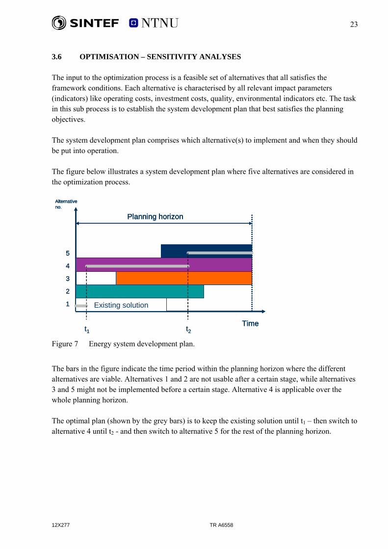
3.6 OPTIMISATION – SENSITIVITY ANALYSES The input to the optimization process is a feasible set of alternatives that all satisfies the framework conditions. Each alternative is characterised by all relevant impact parameters (indicators) like operating costs, investment costs, quality, environmental indicators etc. The task in this sub process is to establish the system development plan that best satisfies the planning objectives. The system development plan comprises which alternative(s) to implement and when they should be put into operation. The figure below illustrates a system development plan where five alternatives are considered in the optimization process.
Existing solution
Alternative no.
2
3
4
5
1
Time
Planning horizon
t1 t2
Existing solution
Alternative no.
2
3
4
5
1
Time
Planning horizon
Existing solution
Alternative no.
2
3
4
5
1
Time
Planning horizon
t1 t2 Figure 7 Energy system development plan.
The bars in the figure indicate the time period within the planning horizon where the different alternatives are viable. Alternatives 1 and 2 are not usable after a certain stage, while alternatives 3 and 5 might not be implemented before a certain stage. Alternative 4 is applicable over the whole planning horizon. The optimal plan (shown by the grey bars) is to keep the existing solution until t1 – then switch to alternative 4 until t2 - and then switch to alternative 5 for the rest of the planning horizon.
12X277 TR A6558

24
12X277 TR A6558
3.7 CORPORATE ECONOMICS – RISK EVALUATION Private and public actors - with limited capital resources - often have other investment opportunities that might compete with the spending of capital resources on a socio-economic efficient energy project. Although the energy authorities motivate energy actors to comply with socio-economic objectives, the regulatory framework might have imperfections. A socio-economic profitable project estimate might not be profitable from a corporate economic point of view – the profit margins might be quite different. In a decision making process corporate economics might prevent a project from being realised. Examples of sources for discrepancies between socio-economics and corporate economics are:
• Differences in interest rates – depreciation times • Cost and profit sharing between stakeholders • Tax effects • Differences in risk attitudes
Interest rates are often used as a tool to manage risk. When the risk is considered to be high, the interest rate in corporate evaluations will be high and the planning horizon short. The rates will normally be higher than the socio- economic prescribed rates. In Norway the Ministry of Finance publish socio-economic interest rates as a combination of a risk free real interest rate and a risk premium. 3.8 CONCESSION PROCESS – EXTERNAL ECONOMICAL SUPPORT
PROCESS(ES) Normally energy projects require license(s) before construction to protect public and private interests. Several acts and regulations might apply and the most important are:
• The Energy Act • The Planning and Building Act. • The Natural Gas Act • The Pollution Control Act • The Watercourse Regulation Act • The Industrial Licensing Act
NVE performs the basic evaluation of applications for licenses related to electricity supply, district heating and natural gas on the Norwegian mainland. Installations that require a license are:
• Electrical installations with a voltage greater than 1000 V AC / 1500 V DC. Electricity network owners have a (general) local area license for electrical installations ≤ 22 kV.
• District heating plants with an output greater than 10 MW (10 MJ/s). • Gas fired power plants and gas distribution installations costing more than 6 million Euros.

25
12X277 TR A6558
As an example of a concession application process and the elements and procedures involved, the following requirements are given in the Energy Act. Application processes under the provisions of other acts use similar principles and requirements. Excerpt from the Energy Act §2.1 (translated from Norwegian): The application shall provide the information that is necessary in order to assess whether a licence should be granted and which conditions shall be specified. ---- Applications that meet the requirements specified in this paragraph shall be distributed for comment in the Norwegian Water Resources and Energy Directorate and in affected municipalities or some other appropriate place in that district. ---- A public announcement of the application, a brief description of the plans, information about where the application has been distributed for comment and the deadline for submitting comments shall be posted in the Official Norwegian Gazette and in one or more newspapers that are commonly read in the district. ---- Public bodies and others to whom the measure directly applies shall have a copy of the application sent to them for comment. When the application is sent out for comment, a deadline will be set for submitting comments to the licensing authority. When it is deemed unobjectionable, a public consultation may be omitted. The processing of an application in accordance with this Act may be postponed pending an energy plan pursuant to section 5B-1. Excerpt from the Energy Act Regulations §3.2: The content of applications for a licence for electrical installations Insofar as it is appropriate, an application for a licence for electrical installations shall include the following items: a) a description of the applicant and his activities b) a technical and economic description of the installation, including the physical design of the
installation and any auxiliary installations such as roads etc. c) how the installation fits into the energy plan d) the planned date for the start-up and completion of the installation e) an account of the installation's adaptation to the landscape with necessary drawings and maps f) the effect on public interests and possible measures to mitigate the impact g) the results of any environmental impact assessments h) the effect on private interests, including the interests of landowners and other holders of rights i) the need for permits pursuant to some other Act, including the relation to municipal plans
pursuant to the Planning and Building Act. During the application process new information might be provided from different stakeholders that might contribute the modification of the project/alternatives to achieve a best possible socio-

26
12X277 TR A6558
economic solution i.e. to take into account all relevant impacts of the different alternatives for all stakeholders affected - as required in socio-economic analyses. The economics in an energy project is a key aspect. As mentioned in section 3.7, in some projects a socio-economic beneficial project might not give sufficient corporate economic incentives to be realised. As a tool to motivate for the realisation of such projects, the Energy Fund is set up by the Norwegian Parliament. The Energy Fund is managed by Enova and might give economic support of energy investments to bridge the gap between socio-economics and corporate economics to promote cost-effective and environmentally sound investments. Hence, in an energy project it might be worth-while to seek for external support from different sources – Enova and others. 3.9 FINAL DECISION – IMPLEMENTATION OF PROJECT The last step in a local energy planning decision process is to decide whether the project should be realised or not. With licences granted and a sound project economy and limited risk in the project, a decision will lead to the implementation phase of the project. This phase involves detailed design, contracting, construction work, acquisitions, quality assurance and similar. In rare cases the findings in the implementation phase might lead to modification of the project as indicated in the flowchart. As an example, if archaeological discoveries are made during excavation works, this might have project effects.

27
12X277 TR A6558
4 PLANNING TOOLS A web-site called ‘Energy Planning Toolbox’ has been created: http://www.energy.sintef.no/prosjekt/energyplanningtoolbox/index.asp The toolbox is created to support and guide the process of planning local energy systems with mixed energy carriers, particularly electricity, gas and hot water. The toolbox gives a comprehensive description of the complex planning process. It includes the main topics from the technical reports illustrated by examples and thus enables users to learn and understand the potential benefits of the different tools which can support the local energy planning process. 4.1 OBJECTIVE OF ENERGY PLANNING TOOLBOX The main objective of the ‘Energy Planning Toolbox’ is to provide support for the analyses and decisions that are required during the planning process and for educational, research and development purposes. This planning toolbox aims at closing the gap between the availability of scientific solutions and their use in practice. The web-site is intended to be an environment for discussions, guidance and decision support in local energy systems planning attempting to close the gap between scientific oriented descriptions and their use in practice. It is designed to meet the demands of both the scientific community (researchers, teachers, students) and of the actual planners (municipalities, local authorities, utilities and other stakeholders). The toolbox is a collection of methodological3 elements developed in the SEDS project and elsewhere. This library or collection of tools includes information about the applicability of the methods, their data requirement and which parts of the planning process these methods can support. Furthermore information or direct links is given of where to find more information about the actual methods, programs, prototypes etc. The library should give an overview of the commercial and internal developed (NTNU&SINTEF) software as well as prototypes, algorithms etc. The ‘Energy Planning Toolbox’ will be a dynamic environment, subject to continuous updating that should be based on an active monitoring of the research developments in the energy planning field.
3 Models, methods, tools, prototypes, procedures, handbooks, guides, examples, data etc.

28
12X277 TR A6558
4.2 USERS The ‘Energy Planning Toolbox’ is designed for different types of users: students, researchers and teachers at the ‘Energy and Environment’ curriculum at NTNU, energy companies, authorities (municipalities) and other entities involved in local energy planning The toolbox gives a comprehensive picture of the planning process and enables its users to learn and understand the potential benefits of the different tools that can support the local energy planning process. In particular:
• Students will be able to: o learn about methods and theory applied in energy systems planning o access case studies and examples related to local energy systems planning o find guidance and supporting material for performing analyses and carrying out
projects and MSc work. • Researchers and teachers at the ‘Energy and Environment’ curriculum will find support
for: o teaching the subject ‘energy planning’ and supervising projects and MSc studies o visualisation and demonstration of planning aspects, mechanisms and ideas o carrying out analyses in energy planning projects o accessing data and specific case-studies o testing of new models and methods.
• Energy companies, authorities and other entities involved in local energy planning will: o get an overview of the useful methodologies and tools for decision analysis and
support that can supplement their existing planning routines o find support for structuring the information and the analysis process in energy
planning study o gain a broader knowledge of the planning process.
4.3 THE CONTENT OF THE ENERGY SYSTEM PLANNING TOOLBOX The research in the field of energy systems planning has always been interdisciplinary, combining concepts and theories from engineering, operations research (economy), system analysis and social science (policy making). The planning toolbox will include methodological elements studied and developed within the SEDS project and elsewhere. The term ‘tool’ in this context refers to any methodological element that can be used in planning, e.g:
• methods • methodologies: it refers to set of methods or more, i.e. the rationale and the philosophical
assumptions that underlie a particular study • mathematical models/algorithms • computer software, prototypes

29
12X277 TR A6558
• case-studies and examples • scientific reports and other studies/reviews • various sources of information/data.
The information contained in the toolbox environment will be presented in form of:
• general descriptions of the main groups of tools • description of the planning methodology developed within SEDS • more detailed descriptions of particular tools, including advantages and disadvantages,
data input and other conditions of use • links to additional information about the tools.
4.4 THE ORGANIZATION OF THE ENERGY SYSTEM PLANNING TOOLBOX 4.4.1 General principles The ‘Energy Planning Toolbox’ offers a comprehensive picture of the planning process and enables different users to learn about and to understand the potential benefits of the different tools that can support the local energy planning process. As mentioned above the toolbox targets different types of users with possibly different views and needs for analysis. Therefore, when structuring the planning toolbox the idea is to cover as much as possible the way different users will need and search for different types of information. Thus, the toolbox is designed on two levels: the first level provides an overview over the energy system planning process while the second level provides an overview of various methods that can be applied in an energy planning study. The two levels are suggestively named ‘Planning tasks’ and ‘Planning tools’ Figure 8 illustrates the content of the two levels.

30
Figure 8 Main levels in the organization of the energy system planning toolbox.
The advantage of this way of structuring will be that a user will get both a picture of the whole complexity of the planning process (a practical approach) and an overview of the different groups of tools that can be used to solve different planning tasks (a more theoretical approach). In order to reach the goal of closing the gap between the availability of scientific solutions and their use in practice it is very important that the tool attracts energy companies, authorities and other entities involved in local energy planning. The advantages the toolbox brings to these users should be twofold. The toolbox should offer an insight into the direct practical use of concepts/methods and an insight into the way of structuring complex projects, in order to achieve consensus among the affected groups and decision makers. The last is the primary requirement for the implementation of the planning results. This section discusses further in details the organization of the energy planning toolbox on the two design levels. A colour-coding scheme is used to mark the correspondence between the two levels. Colours will be used to differentiate among the various planning tasks and to characterize the different tools in the toolbox, as to which task in the planning process the tool covers or is related to.
12X277
TR A6558
31
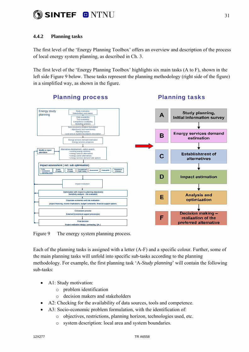
4.4.2 Planning tasks The first level of the ‘Energy Planning Toolbox’ offers an overview and description of the process of local energy system planning, as described in Ch. 3. The first level of the ‘Energy Planning Toolbox’ highlights six main tasks (A to F), shown in the left side Figure 9 below. These tasks represent the planning methodology (right side of the figure) in a simplified way, as shown in the figure.
Planning process Planning tasks
Energy services demand estimationEnergy services prognosis
Alternatives development - option search:• existing energy solutions • energy sources alternatives• energy carrier alternatives• energy services demand side options
Costs- investments- operating costs
Quality of supply
Occupational/Public Safety Environment Political/PR Security
of supplyRegulationsContracts
Modify or reject alternative
Impact assessment ( incl. sub optimisation)
Optimisation with respect to planning objective(s)Sensitivity analysis - risk evaluation
Corporate economics and risk evaluation-
project financing, income implications, budget constraints, financial support options
Concession process
External Economical support process(es)
12X277 TR A6558
Final decision
Project realisation design, contracting, QA..)
Impact evaluation
Study motivation Stakeholders and stakes
Data availabilityTool availability
Competence availabilityModelling ambition
Socio-economic problem formulation- objective(s) and restriction(s)
Planning horizon Local area & System boundaries description
Energy studyplanning
Energy services demand estimationEnergy services prognosis
Alternatives development - option search:• existing energy solutions • energy sources alternatives• energy carrier alternatives• energy services demand side options
Costs- investments- operating costs
Quality of supply
Occupational/Public Safety Environment Political/PR Security
of supplyRegulationsContracts
Modify or reject alternative
Impact assessment ( incl. sub optimisation)
Optimisation with respect to planning objective(s)Sensitivity analysis - risk evaluation
Corporate economics and risk evaluation-
project financing, income implications, budget constraints, financial support options
Concession process
External Economical support process(es)
Final decision
Project realisation design, contracting, QA..)
Impact evaluation
Study motivation Stakeholders and stakes
Data availabilityTool availability
Competence availabilityModelling ambition
Socio-economic problem formulation- objective(s) and restriction(s)
Planning horizon Local area & System boundaries description
Energy studyplanning
Figure 9 The energy system planning process.
Each of the planning tasks is assigned with a letter (A-F) and a specific colour. Further, some of the main planning tasks will unfold into specific sub-tasks according to the planning methodology. For example, the first planning task ‘A-Study planning’ will contain the following sub-tasks:
• A1: Study motivation: o problem identification o decision makers and stakeholders
• A2: Checking for the availability of data sources, tools and competence. • A3: Socio-economic problem formulation, with the identification of:
o objectives, restrictions, planning horizon, technologies used, etc. o system description: local area and system boundaries.

32
12X277 TR A6558
Each planning task/sub-task is separately described. Guidelines and suggestions on how to carry our each specific task are also provides. Moreover, the user can find links to the tools that can be used to solve each specific planning task, such as: methodologies, methods, software, modelling tools, examples and case studies. This way of structuring provides the user with the possibility to unfold the different planning phases and find examples, in-depth information and links to the tools that can support different planning tasks. 4.4.3 Planning tools The second level of the ‘Energy Planning Toolbox’ offers an overview and description of various tools (methods, methodologies, software, sources of information, etc.) that can be used in the planning process. There is no single method or tool that can address the whole complex process of planning energy systems. Usually tools are developed to address one or more parts of the planning process. In the ‘Energy Planning Toolbox’ the tools are organized into the following groups (or categories):
• data sources and load models • impact assessment models • decision support models • case-studies, examples • reports, research papers, other references.
Each group of tools is generally described and links are further provided to the tools that are part to that specific group. Each tool is then separately described with details like:
• a general description and purpose • application domain and which planning task the tool can cover
o what are the previous planning tasks the user should undertake in order to use a tool,
o and which further planning tasks will employ (‘need’) the results obtained with that particular tool
• key elements • benefits • limitations • links to additional information about the tools: research, web-pages, references,
advantages and disadvantages, data input and other conditions of use etc.

33
12X277 TR A6558
4.4.4 User guidance, example To facilitate a better understanding of how to use the Energy Planning Toolbox, examples and case studies are included. They illustrate how to carry out the different planning tasks, and which tools can be used to accomplish these tasks. 4.5 SUMMARY The current toolbox is a preliminary version, particularly concerning the content. The main objective within the SEDS project has been to provide a useful environment for visualization and demonstration of local energy planning with multiple carriers. It is organized along two axes: the main planning tasks and the available tools, focusing on impact evaluation and decision support. A few examples and case studies have been included. The toolbox provides a summary of the results from the SEDS project. It is expected that application of the toolbox will promote more content to be added along both axes, such that the toolbox environment can develop into a useful instrument for teaching and research, as well as for decision makers and stakeholders involved with practical planning.

34
12X277 TR A6558
5 REFERENCES [1] Sand, K.; Holen, A.T.; Kjølle, G.H.; Ulseth, R.; Jordanger, E.: Planning of sustainable energy distribution systems. Part I: Problem definition and planning principles. Trondheim: NTNU/SINTEF Energiforskning, December 2007 (TR A6557) [2] Energy Planning Toolbox web-site:
http://www.energy.sintef.no/prosjekt/energyplanningtoolbox/ [3] Risnes, A. S. R.: SEDS. Gjennomgang av prosjekt- og masteroppgaver i energiplanlegging (in Norwegian). Trondheim: NTNU/SINTEF Energy Research 2005 (AN 05.12.55) [4] Catrinu, M. D.: Decision Aid for Planning Local Energy Systems. Doctoral theses at NTNU, 2006:62, April 2006. [5] Botterud, A., Catrinu, M. D., Wolfgang, O., Holen, A.T.: Integrated Energy System
Planning: A Multi-Criteria Approach. Proceedings of the 15th Power Systems Computation Conference, (PSCC2005) Liege,
Belgium, August 2005. [6] Løken, E., Botterud, A., Holen, A.T.: Decision Analysis and Uncertainties in Planning
Local Energy Systems. Proceedings of Probability Methods Applied to Power Systems (PMAPS 2006),
Stockholm, June 2006. [7] Løken, E., Botterud, A., Holen, A.T.: Use of Equivalent Attribute Technique in Multi-
Criteria Planning of Local Energy Systems. Proceedings of Operational Research Models and Methods in the Energy Sector
(ORMMES’2006), Portugal, September 2006. [8] Matos, M. A.: Tutorial on Application of Risk Analysis and Multi-Criteria Models in
Energy Systems Planning. NTNU, Trondheim, 6-9 October 2003. [9] Planleggingsbok for Kraftnett, Sintef Energy Research. (In Norwegian).

35
12X277 TR A6558
[10] Skjelbred, H.I., Wolfgand, O.: Energitransport i Stjørdal. (In Norwegian) Trondheim: SINTEF Energy Research 2005 (TR A6217) [11] Quality of electricity supply: Initial benchmarking on actual levels, standards and regulatory strategies, Council of European Energy Regulators Working Group on Quality of Electricity Supply April 2001 [12] Anne Sofie Risnes, Stig J. Haugen: Veileder for kraftsystemutredninger. (In Norwegian) Veileder nr 2 2007, NVE [13] Forskrift om leveringskvalitet i kraftsystemet. (In Norwegian) Available online: www.lovdata.no or www.nve.no [14] Official Norwegian Report NOU 2006:6: When security is the most important (in
Norwegian) [15] EU Commission: On a European Programme for Critical Infrastructure Protection, Green
Paper (COM (2005) 576), Brussels 2005-11-17 [16] EU Directive 2005/89/EC of 18 January 2006 concerning measures to safeguard security
of electricity supply and infrastructure investment [17] EU Directive 2004/67/EC of 26 April 2004 concerning measures to safeguard security of
natural gas supply [18] Doorman G., Uhlen, K., Kjølle, G. H., Huse, E. S.: Vulnerability Analysis of the Nordic
Power System, IEEE Trans. on Power Systems, Vol. 21, No. 1, Febr. 2006 [19] Kjølle, G., Ryen, K., Hestnes, B., Ween, H. O.: Vulnerability in electric power networks
NORDAC, Stockholm, August 2006 [20] Vessia, Ø.: Planning of sustainable energy distribution systems. Part III: A life cycle assessment perspective. Trondheim: NTNU/SINTEF Energiforskning, December 2007 (TR A6560) [21] Holen, A.T.; Kjølle, G.H.: Planning of sustainable energy distribution systems. Executive summary. Trondheim: NTNU/SINTEF Energiforskning, December 2007 (TR A6556)


Appendix 1: Decision makers, Stakeholders and stakes 37
12X277 TR A6558
APPENDIX 1: DECISION MAKERS, STAKEHOLDERS AND STAKES
TABLE OF CONTENTS Page
A1.1 INTRODUCTION .............................................................................................................38
A1.2 DECISION MAKERS.......................................................................................................38
A1.3 ENERGY DISTRIBUTION COMPANIES......................................................................39 A1.3.1 TASKS AND STAKEHOLDERS ......................................................................39 A1.3.2 CHALLENGES...................................................................................................40
A1.4 NVE (REGULATORY BODY)........................................................................................40 A1.4.1 TASKS AND STAKEHOLDERS ......................................................................41 A1.4.2 CHALLENGES...................................................................................................42
A1.5 ENOVA SF (GOVERNMENTAL AGENCY) .................................................................42 A1.5.1 TASKS AND STAKEHOLDERS ......................................................................42 A1.5.2 CHALLENGES...................................................................................................43
A1.6 MUNICIPALITIES AND COUNTIES (LOCAL AND REGIONAL GOVERNMENTS)............................................................................................................43 A1.6.1 TASKS AND STAKEHOLDERS ......................................................................43

Appendix 1: Decision makers, Stakeholders and stakes 38
12X277 TR A6558
A1.1 INTRODUCTION This appendix gives an overview of planning problems and tasks as well as challenges for the most important groups of decision makers in the planning of local energy system. The discussion further will focus on examples form the Norwegian energy sector. A1.2 DECISION MAKERS There are many stakeholders involved in local energy system planning, influencing the decisions to a different degree. The number of decision makers involved in the planning of local energy distribution networks will depend on the actual situation at the specific location. However, in general four important groups of decision makers may be identified:
• Energy distribution companies • Regulatory bodies (NVE) • Governmental agencies (ENOVA) • Local and regional governments (municipalities and counties)
Distribution companies for different energy carriers constitute the most obvious group, as these companies make the investment decisions. Since distribution of energy can be viewed as a natural monopoly, the system regulators will play a crucial role in deciding a regulatory framework, through which the distribution companies are given the correct incentives to invest in new infrastructure. When several energy carriers are involved, there is a challenge for the regulators to design a consistent set of rules, which takes into account the interplay between the energy carriers. The Norwegian Water Resources and Energy Directorate (NVE) is the system regulator in Norway. Enova SF is a governmental agency in Norway regarding use and production of energy. Enova’s main role is to promote and fund energy solutions according to the energy policy of its owner, the Royal Norwegian Ministry of Petroleum and Energy. Local and regional governments (municipalities and counties) will have an important role as a decision maker in the local energy system. In many countries it is common that municipalities and counties own the energy distribution companies (at least partly). Hence, these authorities can also exert direct control on the investment decisions. The following chapters describe tasks and related challenges for the four groups of decision makers mentioned above.

Appendix 1: Decision makers, Stakeholders and stakes 39
12X277 TR A6558
A1.3 ENERGY DISTRIBUTION COMPANIES The energy distribution companies in Norway are monopolies within their areas regarding construction and operation of the electricity distribution system with a nominal voltage up to and including 22 kV. This is according to the local area license. A few companies have also production and distribution of district heating and distribution of natural gas. District heating plants with an output greater than 10 MW (10 MJ/s), and gas fired power plants and gas distribution installations costing more than 6 million Euro require license. A1.3.1 TASKS AND STAKEHOLDERS The following three tasks at the energy distribution companies are relevant in local energy planning:
1. Planning and design of distribution systems for electricity, district heating and natural gas (new installations as well as enlargement and renewal of existing installations). − Load estimation − Technical analyses (present and future quality of supply) − Economical analyses (profitability)
2. Local energy planning (surveys). The local area concessionaires shall prepare, annually
update and make public an energy plan for each municipality in the concession area. Such a plan shall contain the description of: − The current energy system and the energy supplies in the municipality − Expected stationary energy demand in the municipality − The most relevant energy solutions for areas in the municipality − The possibilities for distributed generation (small power plants)
3. Coordinated power systems planning in the regional and the central grid system (surveys).
Energy distribution companies which are appointed as planning coordinators shall annually prepare and publish an updated power system plan for its planning area containing the description of: − Planning assumptions − The current power supply system − Future transmission conditions − Measures and investments
Stakeholders seen from the energy distribution companies regarding the three tasks are:
• Local and regional governments (municipalities and counties) • NVE • Enova • Statnett (transmission system operator) • Consultants

Appendix 1: Decision makers, Stakeholders and stakes 40
12X277 TR A6558
• Suppliers, contractors • End-users
A1.3.2 CHALLENGES There are different challenges for the energy distribution companies related to the three tasks in the previous chapter:
• An energy distribution company with concession for district heating has supply duty. The end-users have connection duty in accordance with the planning- and building law (§ 66a), but no duty regarding use of district heating. This results in uncertainty in the dimensioning of the electricity network when taking into account the effect of the district heating.
• Introduction of district heating and gas distribution which substitute use of electricity in an area may reduce the needs for measures in the electricity distribution. The utilization of reduced power demand in reducing power network costs may be difficult since the requirements to the electricity distribution system will remain the same.
• Introduction of district heating and gas distribution may also contribute to a more flexible and robust energy distribution system, but the utilization of different energy carriers for this purpose should be improved.
• Conflicting economical interests between the electricity distribution company and the district heating company in the same corporation may exist.
• Municipality decided energy solutions (e.g. district heating) for a certain area may have negative socio-economic consequences.
• Investments in local generation with negative corporate profitability may have positive socio-economic profitability due to reduced needs for reinforcement in the regional or central grid.
• The energy distribution companies may have problems in prioritising end-user measures ahead of measures in the electricity distribution system.
• Distribution of district heating and natural gas to an area makes it more difficult to estimate the energy and power demand, including the composition of the energy carriers, compared to only electricity supply.
A1.4 NVE (REGULATORY BODY) The Norwegian Water Resources and Energy Directorate (NVE) is subordinated to the Ministry of Petroleum and Energy. NVE is responsible for the administration of Norway´s water and energy resources. The goals of NVE are to ensure consistent and environmentally sound management of water resources, promote an efficient energy market and cost-effective energy systems, and contribute to the economic utilization of energy.

Appendix 1: Decision makers, Stakeholders and stakes 41
12X277 TR A6558
A1.4.1 TASKS AND STAKEHOLDERS The following four tasks of NVE are relevant in local energy planning:
1. Preparation of guidelines for local energy planning (surveys). The local area concessionaires shall prepare, update annually and make public an energy plan for each municipality in the concession area (task 2 in Chapter 1.3.1) containing description of: − The current energy system and the composition of energy in the municipality. − Expected stationary energy demand in the municipality. − The most relevant energy solutions for areas in the municipality. − The possibilities for distributed generation (small power plants).
2. Preparation of guidelines for power system planning in the regional and the central grid
system (surveys). Energy distribution companies which are appointed as planning coordinators shall annually prepare and publish an updated power system plan for its planning area (task 3 in Chapter 1.3.1) containing description of: − Planning assumptions. − The current power supply system. − Future transmission conditions. − Measures and investments.
3. Concession management. NVE performs the basic evaluation of applications for licenses
related to electricity supply, district heating and natural gas on the Norwegian mainland. Installations that require a license are: − Electrical installations with a voltage greater than 1000 V AC / 1500 V DC. Electricity
network owners have a (general) local area licenses for electrical installations ≤ 22 kV. − District heating plants with an output greater than 10 MW (10 MJ/s). − Gas fired power plants and gas distribution installations costing more than 6 million
Euro.
4. Power network analyses as a basis for the evaluation of applications for licenses, etc.: − Load flow calculations. − Reliability calculations. − Socio-economic calculations.
Stakeholders seen from NVE regarding the four tasks are:
• Governmental offices • Energy distribution companies • Enova • Consultants • Research institutions • Statnett (transmission system operator) • Statistisk sentralbyrå (Statistics Norway)

Appendix 1: Decision makers, Stakeholders and stakes 42
12X277 TR A6558
A1.4.2 CHALLENGES The challenges for NVE related to the four tasks in the previous chapter can be summarized as follows:
• Develop criteria, requirements and guidelines for the energy distribution companies that ensure cost-effective energy systems, and contribute to a sound socio-economic and environmentally friendly energy system.
• Request the energy distribution companies to include (more) alternatives in the applications for licenses that are socio-economic cost-effective solutions.
• Develop appropriate and proper measures to follow up and perform control with the energy distribution companies regarding the given requirements.
• Electricity distribution system (MV and LV) planning is not covered by the guidelines for local energy planning and power system planning. The first one is on municipality level and the other on the regional and the central grid system level.
A1.5 ENOVA SF (GOVERNMENTAL AGENCY) Enova SF is a public enterprise owned by the Royal Norwegian Ministry of Petroleum and Energy. Enova`s main mission is to contribute to environmentally sound and rational use and production of energy, relying on financial instruments and incentives to stimulate market actors and mechanisms to achieve national energy policy goals. A1.5.1 TASKS AND STAKEHOLDERS Enova manages the Energy Fund set up by the Norwegian Parliament and finances programmes and initiatives that support and underpin national objectives. Enova has the freedom to choose its policy measures and the responsibility to establish incentives and financial funding schemes that will result in cost effective and environmentally sound investments. The following four tasks at Enova are relevant in local energy planning:
1. Economic support of energy investments. − Applicants are energy production and distribution companies, industrial companies,
municipalities, building owners, individuals, etc. 2. General support arrangements for households.
− From October 2006 households can apply for economic support when purchasing stoves and boilers fired with pellets, energy control systems and large heat pumps.
3. Preparation of criteria for economic support of energy investments. 4. Preparation of guidelines regarding use and production of energy, being a premise
provider.

Appendix 1: Decision makers, Stakeholders and stakes 43
12X277 TR A6558
Stakeholders seen from Enova regarding the four tasks are:
• Governmental offices • NVE • Energy distribution companies • Municipalities • Industrial companies • Consultants • Research institutions • Individuals
A1.5.2 CHALLENGES Challenges for Enova related to the four tasks in the previous chapter may be summarized as follows:
• Consider the socio-economic cost-benefit of projects where applicants have based the application on corporate economic cost-benefit analyses. What are the contributions to the overall objectives?
• Prioritizing economical profitable projects versus less profitable projects which provide new energy supply (kWh).
• Estimate the economic and, environmental impacts and the effect on the local grid from local energy solutions and end-user measures.
• Estimate the impact on the regional and central grid from local energy solutions and end-user measures.
• Interface problems when defining system boundaries. A1.6 MUNICIPALITIES AND COUNTIES (LOCAL AND REGIONAL
GOVERNMENTS) The local governments in Norway are the municipalities while the counties are the regional governments. At present Norway have 431 municipalities and 19 counties. A1.6.1 TASKS AND STAKEHOLDERS The following three tasks at municipalities and counties are relevant in local energy planning:
1. Management of the Planning and building law. 2. Development and follow up of local development plans on municipality level. 3. Development and follow up of regional plans on county level.

Appendix 1: Decision makers, Stakeholders and stakes 44
12X277 TR A6558
Stakeholders seen from municipalities and counties regarding the three tasks are:
• Energy distribution companies • Governmental offices • Enova • Industrial companies • Consultants • Individuals • NVE.
Limited resources and competence regarding energy problems may be a challenge for municipalities and counties related to the tasks described above..

Appendix 2: Load modelling 45
12X277 TR A6558
APPENDIX 2: LOAD MODELLING
TABLE OF CONTENTS Page
A2.1 INTRODUCTION .............................................................................................................46
A2.2 LOAD MODELLING FOR LOCAL ENERGY PLANNING..........................................47 A2.2.1 QUALITY OF LOAD MEASUREMENTS .......................................................47 A2.2.2 FACTORS THAT INFLUENCE ENERGY DEMAND ....................................48
A2.3 SHORT REVIEW OF METHODS FOR LOAD MODELING........................................48 A2.3.1 STATISTICAL ANALYSES..............................................................................49 A2.3.2 ENERGY SIMULATION PROGRAMS............................................................49 A2.3.3 INTELLIGENT COMPUTER SYSTEMS .........................................................49 A2.3.4 SHORT COMPARISON OF METHODS ..........................................................50
A2.4 LOAD MODELLING IN MIXED DISTRIBUTION SYSTEMS....................................50 A2.4.1 MODELLING THE SIMULTANEOUS HEAT AND ELECTRICITY
DEMAND IN BUILDINGS................................................................................50 A2.4.2 RELATIVE LOAD PROFILE ALGORITHM (FOR ONE BUILDING) ..........52 A2.4.3 GENERALIZED LOAD PROFILE ALGORITHM...........................................54 A2.4.4 LOAD AGGREGATION....................................................................................55
A2.5 REFERENCES ..................................................................................................................56
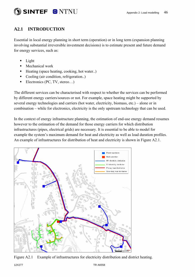
Appendix 2: Load modelling 46
A2.1 INTRODUCTION Essential in local energy planning in short term (operation) or in long term (expansion planning involving substantial irreversible investment decisions) is to estimate present and future demand for energy services, such as:
Light Mechanical work Heating (space heating, cooking, hot water..) Cooling (air condition, refrigeration..) Electronics (PC, TV, stereo…)
The different services can be characterised with respect to whether the services can be performed by different energy carriers/sources or not. For example, space heating might be supported by several energy technologies and carriers (hot water, electricity, biomass, etc.) – alone or in combination – while for electronics, electricity is the only upstream technology that can be used. In the context of energy infrastructure planning, the estimation of end-use energy demand resumes however to the estimation of the demand for those energy carriers for which distribution infrastructures (pipes, electrical grids) are necessary. It is essential to be able to model for example the system’s maximum demand for heat and electricity as well as load duration profiles. An example of infrastructures for distribution of heat and electricity is shown in Figure A2.1.
Figure A2.1 Example of infrastructures for electricity distribution and district heating.
12X277 TR A6558

Appendix 2: Load modelling 47
12X277 TR A6558
Load models can be used to forecast the energy demand both in short term operation of an energy system and in long term expansion planning involving substantial irreversible investment decisions. Load modelling can be defined as aggregation of spatial, individual energy demand specified in time. In practice this is done by establishing representative load profiles for defined customer categories with similar demand. In a PhD study carried out within the SEDS project the objective was to develop a new methodology for load modelling of buildings in mixed energy distribution systems [1]. This thesis made specific contributions by proposing the following:
Models of the simultaneous heat and electricity demand in buildings; a procedure for analysing relative heat and load profiles for each building; a procedure for comparison and generalization of different load profiles for selected
building categories, a procedure for the aggregation of load profiles for a specific planning area (such as in
Figure A2.1) with a given mixture of buildings. The material presented in this appendix is mainly extracted from this PhD study. First, the background information for load modelling is discussed, then a short review of methods for load modelling is given and at the end the thesis contributions are shortly summarized. In addition, a case study presented in Appendix 5 shows how the proposed generalized load profiles can be applied to a specified planning area. A2.2 LOAD MODELLING FOR LOCAL ENERGY PLANNING The information necessary in load modelling is of different nature. Two important ‘ingredients’ are needed when building models for modelling and forecasting energy demand. One is to observe how much and how energy is actually consumed in the area for which the model is built, and to collect measurements in different periods of time. The second one is to try to identify which are the factors that can influence the energy demand and to estimate parameters that can be taken into consideration when modelling this demand. A2.2.1 QUALITY OF LOAD MEASUREMENTS Critical for the validation and use of a load model is to have access to quality load measurements. Collection of data, qualitative verification of data by inspection and the quality assurance of collected data are important steps when using load measurements. Over the last years, automatic hourly measurements of energy consumption have become more widely available, at least for large buildings. The hourly district heat measurements comprise for example the end-uses space heating, ventilation heating and heating of tap water, whereas the hourly electricity measurements comprised the end-uses lighting, pumps, fans and electrical appliances. However, the accuracy of

Appendix 2: Load modelling 48
12X277 TR A6558
the instruments used can induce a degree of uncertainty in measurement that will propagate further into the load model [1]. A2.2.2 FACTORS THAT INFLUENCE ENERGY DEMAND Equally important is the estimation of relevant parameters that may have an influence on the energy demand: climatic parameters, technical parameters of the buildings/installations and social parameters (behavioural determinants). One of the main tasks in load modelling is to investigate the correlation between climatic parameters and the hourly energy consumption. The most common climatic parameters considered in load estimations are: outdoor temperature (daily mean temperature, temperature variations throughout the day), hours of sunlight, wind speed and direction. Physical determinants (e.g. building envelope) and control regimes (the operation of the space heating, the ventilation and the lighting system) are some of the technical parameters that have an influence on load and energy demand in buildings. Construction year, rehabilitation and insulation standards have also been found to be important input parameters in relation to load modelling of buildings, especially for heat purposes. Therefore future developments in building code regulations and the introduction of new technologies regarding energy distribution and conversion (use) will influence the heat and electricity load profiles for new and rehabilitated buildings. Central control and monitoring systems are becoming more widespread in buildings and this has a direct influence on load profiles. For example, control regimes for the ventilation systems are strongly related to the building’s usage time, as well as the indoor air quality control categories that have been applied to ventilation systems. In the end however, the amount of energy used is very dependent upon the attitude and the awareness of energy customers. Consumer’s influence varies, depending on what kind of building they spend their time in. The consumption patterns in different building types, especially in households are unique. In public buildings with automatic control, on the other hand, consumer’s influence can be lower. The awareness and consumer’s attitudes towards energy consumption have also an influence on energy use, especially in households. Theoretically, the price sensitivity of electricity consumers regarding time differentiated tariffs and the customer’s response to strongly increased tariffs should also be taken into consideration in load estimations. However, in the study reported in [2] it is found that residential electricity consumers are not very price responsive. A2.3 SHORT REVIEW OF METHODS FOR LOAD MODELING There are three main methodological approaches to energy estimations and load modelling: statistical analyses, energy simulation programs and intelligent computer systems. These methodologies differ in terms of the input data they require and their applicability [1].

Appendix 2: Load modelling 49
12X277 TR A6558
A2.3.1 STATISTICAL ANALYSES This group of methods comprise: basic statistics, regression analysis, continuous probability distributions. A statistical analysis approach to load modelling requires large amounts of measurements of energy use. The probability sample must have a high level of statistical significance in order to provide a relevant interpretation of the evolution of load and energy demand. Linear or multivariate regression analyses or probability distributions are usually used for load and energy predictions. A regression analysis expresses the mathematical correlation between different variables (e.g. climatic or behavioural factors). A selection of relevant load modelling tools based on statistical analysis methods is presented in [1]. The review includes general descriptions and a comparison of the following methods: ARX model, Conditional demand analysis (CDA), Energy signature, EModel, The Finnish load model and USELOAD. A2.3.2 ENERGY SIMULATION PROGRAMS Energy simulation programs mainly model energy conservation in buildings, including losses (transmission, ventilation and infiltration losses). Two modelling techniques are mainly used in simulation programs: analytical methods – the response function method-, and numerical methods. The response factor method solves linear differential equations that include time invariant parameters while numerical methods can handle nonlinear, time varying equation systems. In general numerical methods are preferred although the analytical programs based on the response function method are easier to validate. Examples of energy simulation programs are: DOE-2, the Engineering Model –EM, ESP-r, EnergyPlus and FRES. References to these methods can be found also in [1], where also several hybrid methods are described. These methods are derived form a combination of statistical analyses and simulation programs. A2.3.3 INTELLIGENT COMPUTER SYSTEMS Expert systems and artificial neural networks can be used for the prediction of energy demand. Expert systems ‘make decisions’ based on interpretation of data and a selection among alternatives. Neural networks are used to make predictions based on a set of data. The approach is suited for load modelling and energy estimations because it is able to handle incomplete data which might result form measured energy data and climatic parameters. Neural networks are trained in relation to a set of data until the network recognizes the patterns presented, and then it is capable of making predictions based on new patterns.

Appendix 2: Load modelling 50
12X277 TR A6558
A2.3.4 SHORT COMPARISON OF METHODS Usually the amount of data required by a method differs according to the accuracy level of the calculations [1]. For example statistical analyses primarily need load measurements but climatic parameters and some background information on the measured buildings are also important. Simulation programs on the other hand do not require load measurements but climatic parameters and detailed information about the characteristics of the buildings is very important. They also require information about consumer behaviour (i.e. behavioural determinants). Intelligent computer systems process measured load data, climatic parameters, behavioural determinants and background information about the buildings. The more accurate the information provided to the intelligent computer systems is, the better results the solution algorithms will give. This is also true for statistical analyses and simulation programs because the quality of the input data will automatically be reflected in the quality of the results. The methodologies mentioned above can provide both short-term and long-term predictions for load and energy demand. Long-term predictions are the most interesting from the energy planner’s point of view. The uncertainty factors concerning the input parameters are important to be acknowledged especially regarding the climatic representation. Statistical analyses are primarily used in load modelling and energy estimations involving several customers. Because of the detailed nature of simulation programs, these tools are applicable for one or a few large customers. For example simulation programs are very good at analysing retrofitting options of already existing buildings. In some situations these tools may be used to model several customers, but the output would be purely theoretical, and not the real behaviour of the buildings. The application of intelligent computer systems may be used on the building level as well as the regional and national level. A2.4 LOAD MODELLING IN MIXED DISTRIBUTION SYSTEMS A2.4.1 MODELLING THE SIMULTANEOUS HEAT AND ELECTRICITY DEMAND
IN BUILDINGS A2.4.1.1 The heat load model In order to model the heat load, a new procedure has been developed to determine the change-point temperature for dividing temperature-independent heat consumption such as space heating, ventilation and hot tap water. The background for the load model has been hourly load measurements of various buildings in Trondheim and Bergen, Norway. The hourly district heat measurements comprised the end-uses space heating, ventilation heating and heating of tap water.

Appendix 2: Load modelling 51
In order to be able to model the heat load, a distinction had to be made between temperature-dependent and temperature-independent district heat consumption; hence, the different parts had to be analyzed separately. Figure A2.2 illustrates the difference between temperature-dependent and temperature-independent district heat consumption. When modelling, the change-point temperature has to be found, i.e. the daily mean temperature separating the temperature-dependent and temperature-independent district heat consumption.
12X277 TR A6558
-200
-15 -10 -5 0 5 10 15 20 25
100
200
300
400
500
600
700
Daily mean temperature [degree Celsius]
Dis
trict
hea
t con
sum
ptio
n [k
Wh/
h]
Hourly district heat consumption for OB2; 11 a.m. to 12 p.m.
Weekdays
Temperature dependent district heat consumption
Temperature independent district heat consumption
-200
-15 -10 -5 0 5 10 15 20
100
200
300
400
500
600
700
25Daily mean temperature [degree Celsius]
Dis
trict
hea
t con
sum
ptio
n [k
Wh/
h]
Hourly district heat consumption for OB2; 11 a.m. to 12 p.m.
Weekdays
Temperature dependent district heat consumption
Temperature independent district heat consumption
Figure A2.2 Scatter plot of daily mean temperature vs. hourly district heat consumption for OB2
in Trondheim for weekdays hour 12, i.e. district heat consumption from 11 a.m. to 12 p.m. for nearly five years (January 2002 – October 2006) [1].
The heat load model is based on piece-wise linear regression analyses for every hour of the day and day type. The day types are divided into weekdays (Mondays through Fridays) and weekends/holidays (Saturdays and Sundays) because significantly different load profiles correspond to the various day types. The mathematical procedure developed to find the change-point temperature for a given building at a given hour is based on a linear regression equation:
Yi = α + β · xi + ei where xi is the independent regressor variable, Yi is the dependent random variable and ei is called the residual and describes the error in the fit of the model. α- and β-are called regression coefficients. The estimation of α- and β coefficients for sets of measured data, is the core of the proposed methodology. The change-point temperature is found by assuming a linear correlation between hourly district heat consumption and daily mean temperature. The regression coefficients α and β are calculated for temperature steps of 0.1°C, starting at a daily mean temperature of 17°C and stepping down to 0°C. The change-point temperature is found in the range where the β-values fluctuated least, i.e. an approximately constant β-value indicates that the influence of the temperature-independent

Appendix 2: Load modelling 52
12X277 TR A6558
heat consumption is neglectable. For more information concerning the mathematical procedure and the verification of the heat load model, see [1]. Relative design heat load profiles for several buildings within a certain building category are derived in order to compare and generalize the heat load profiles. The relative load profiles are found by dividing the design heat load for each hour and day type by the average design load. The relative heat load profiles for the temperature-independent season are also found by dividing the expected values for each hour and day type by the average design load. In order to generalize the heat load profiles for different building categories, it is very important to sort the buildings into different archetypes regarding building type and regulation regime. When the buildings analyzed have been classified according to archetype, the relative expected value for each archetype is calculated based on each building’s relative expected value. A2.4.1.2 The electricity load model The electricity consumption has been investigated in relation to various seasons, as well as day types and hour of the day. The analyses revealed that there are some seasonal variations in electricity consumption which could not be related only to the outdoor temperature alone. For example, lighting as an end-use is related to seasonal changes in hours of daylight and sun. Pumps and fans as end-uses are related to space heating and ventilation heating systems. The amount of electricity for the pumps is decreased during the temperature-independent season, only circulating hot tap water. The supply air rate in the ventilation system is independent of climatic conditions and strongly related to the building’s utilization time. Electrical appliances are related to work-hours and behavioural determinants. The electricity load model is based on continuous probability distribution analyses for every hour of the day and day type. The hourly electricity consumption data for each day type is mainly examined in relation to normal, lognormal and Student’s t distributions. Relative electricity load profiles are found by dividing the seasonal load for each hour j and day type d by the average design load for electricity. Then, the same generalization procedure which was applied to the heat load profiles is also applied to the electricity load profiles. Generalized load profiles are calculated for every building category or archetype for each season and day type. The mathematical procedure and examples of electricity load profiles are detailed in [1]. A2.4.2 RELATIVE LOAD PROFILE ALGORITHM (FOR ONE BUILDING) The procedure for the solution algorithm for relative load profiles (heat and electricity) for one building can be summarized as in Figure A2.3.
1. Load specific building file and perform quality assurance on the data.
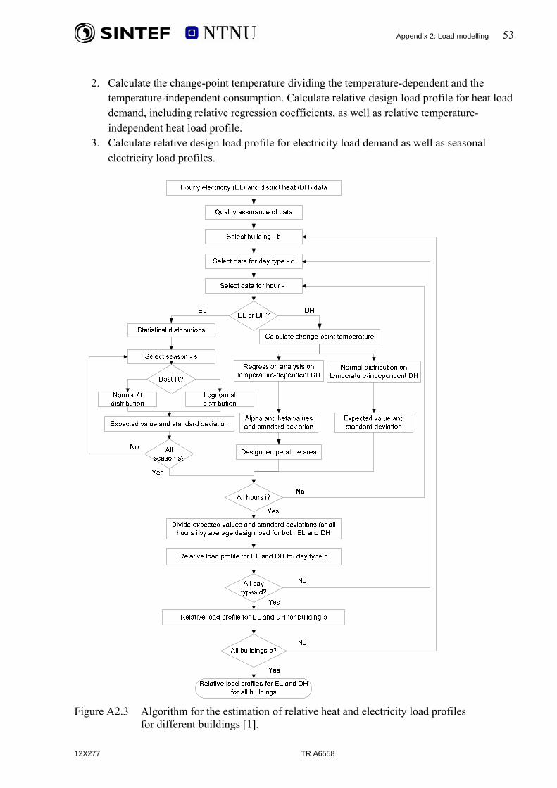
Appendix 2: Load modelling 53
2. Calculate the change-point temperature dividing the temperature-dependent and the temperature-independent consumption. Calculate relative design load profile for heat load demand, including relative regression coefficients, as well as relative temperature-independent heat load profile.
3. Calculate relative design load profile for electricity load demand as well as seasonal electricity load profiles.
Figure A2.3 Algorithm for the estimation of relative heat and electricity load profiles
for different buildings [1].
12X277 TR A6558

Appendix 2: Load modelling 54
A2.4.3 GENERALIZED LOAD PROFILE ALGORITHM The algorithm for generalised heat and electricity load profiles have been developed for various building categories, such as single family houses and apartment blocks, office buildings, educational buildings, hotels and restaurants. The procedure for the solution algorithm for generalized load profiles for different building categories/archetypes proposed in [1] is as following:
1. Load relative heat and electricity load profiles for all buildings analyzed. 2. Sort load profiles by building category and archetype. 3. Calculate expected value and standard deviation for all archetypes.
Figure A2.4 Algorithm for the generalization of relative heat and electricity load profiles for a given building category or archetype [1].
12X277 TR A6558

Appendix 2: Load modelling 55
12X277 TR A6558
Also, the division of buildings into different archetypes has been identified in relation to load profiles, especially for heat load profiles in educational buildings. The building’s age and whether or not it has been subject to rehabilitation play a very important role in determining the generalised load profile’s categorization, and not just the building category. A2.4.4 LOAD AGGREGATION A bottom-up approach has been applied for the aggregation of individual building load profiles in order to derive the heat and electricity load profiles for a specified planning area supplied by district heating and electricity (example in Figure A2.1). The procedure for the solution algorithm for aggregation of load profiles for a specified planning area with a given mixture of buildings is as following:
1. Select a specific planning area (example in Figure A2.1) with a defined mixture of buildings.
2. Apply generalized heat and electricity load profiles for building b based on the building category.
3. Use specific load indicators to construct real heat and electricity load profiles as well as standard deviations for design day.
4. Apply design reference year (DRY) for calculating relative yearly load profiles. Use specific energy indicators to calculate real yearly heat and electricity load profiles.
5. Add real design heat and electricity load profiles at node connection points as well as standard deviations. Add yearly load profiles at the same node.
6. Add all design and yearly load profiles at the energy distribution/transformer unit, including a 95% quantile for peak load estimations.
7. Calculate coincidence factor for heat and electricity for design load profiles. 8. Choose energy carriers and include distribution losses for maximum load and annual
energy accordingly.

Appendix 2: Load modelling 56
Figure A2.5 Algorithm for the aggregation of generalized heat and electricity load profiles and energy demand for a specified planning area including distribution load and energy losses [1].
A2.5 REFERENCES [1] Pedersen L: Load modelling of buildings in mixed energy distribution systems Doctoral thesis at NTNU, 2007:78, February 2007. [2] Ericson, T.: Short-term electricity demand response Doctoral thesis at NTNU, 2007:53, February 2007.
12X277 TR A6558
Appendix 3: Multi-criteria decision aid for energy planning 57
12X277 TR A6558
APPENDIX 3: MULTI-CRITERIA DECISION AID FOR ENERGY PLANNING
TABLE OF CONTENTS Page
A3.1 INTRODUCTION .............................................................................................................58 A3.1.1 SHORTLY ABOUT MCDA...............................................................................58
A3.2 APPLYING MCDA IN ENERGY PLANNING...............................................................60 A3.2.1 PROBLEM STRUCTURING .............................................................................60 A3.2.2 MODELLING .....................................................................................................60
A3.2.2.1 Impact modelling..............................................................................61 A3.2.2.2 Preference modelling and analysis using MCDA.............................63
A3.2.3 DERIVING RECOMMENDATIONS ................................................................66
A3.3 DATA REQUIREMENT AND CATEGORIES...............................................................68 A3.3.1 LOAD..................................................................................................................68 A3.3.2 ENERGY TRANSPORT SYSTEM....................................................................69 A3.3.3 GENERATION, CONVERSION AND STORAGE TECHNOLOGIES...........69 A3.3.4 EMISSIONS........................................................................................................69 A3.3.5 RELIABILITY AND QUALITY........................................................................69 A3.3.6 COSTS AND PRICES ........................................................................................70
A3.4 REFERENCES ..................................................................................................................71

Appendix 3: Multi-criteria decision aid for energy planning 58
12X277 TR A6558
A3.1 INTRODUCTION The process of decision making for local energy systems planning is complex. Decentralization, the interplay between different energy and emission markets, and the movement toward sustainability have changed the priorities of energy planners and policy makers. Therefore, in most situations the economic, environmental, political or social impacts of different decisions must be carefully estimated and evaluated simultaneously. Multi-criteria decision analysis is a discipline that has a lot to offer when it is necessary to tackle the complex decision situations when planning sustainable energy systems. The purpose of this appendix is to give an overview and description of the main elements when using multi-criteria decision aid for planning. The material in this appendix is extracted from two PhD studies carried out at NTNU: one was part of the SEDS project [1] and the other was part of another project, connected to SEDS, ‘Analysis of energy transport systems with multiple energy carriers’ (eTransport) [2] [3]. The research has partly been presented at conferences, workshops and in scientific journals. A3.1.1 SHORTLY ABOUT MCDA Multi-Criteria Decision Analysis (MCDA) is an alternative to the traditional analysis methods (e.g. cost-benefit analysis) used for decision support. Multi-Criteria Decision Analysis (MCDA) is the discipline that studies methods and procedures by which concerns about multiple conflicting criteria can be formally incorporated into the management planning process. A review of MCDA methods can be found in [1] and [2]. The use of MCDA in energy systems planning is justified by the simple fact that not all aspects that matter (and must be considered) in distribution system asset management can easily be given a monetary value. When using MCDA light can be shed on what tradeoffs, uncertainties and value judgments are crucial to the decision and what issues do not matter. MCDA is a process which seeks to help decision makers (DMs) learn about and better understand the problem they face, their own values and priorities and the different perspectives of other stakeholders. It is important however to stress the fact that MCDA does not provide ‘the right answer’, as some mathematical or engineering methods would be expected to do. Instead it provides recommendations or advice regarding which decision to make based on the information available in a given decision situation. Practice showed that MCDA’s recommendations are often at least as good as the choices based on intuition (as most decisions are made). The MCDA process (Figure A3.1) starts with problem identification and structuring. Sometimes, in real-life decision situations goals are not so clear, nor the options that will satisfy these goals in

Appendix 3: Multi-criteria decision aid for energy planning 59
the long run. MCDA can thus help decision makers in understanding what they really want to do, ensuring that they look at the ‘right problem’. The next step is modelling. There are two types of modelling for MCDA: the modelling of consequences (impacts) each decision may have in terms of the relevant goals and the modelling of decision-makers’ preferences regarding their options (decision alternatives) with respect to the chosen goals.
Identification of :Key issuesGoalsCriteria/objectivesAlternativesStakeholdersUncertaintiesConstraints
Problem structuring
ConsequencesDM’s values
and preferences
Modeling
Based on:Total valuesDecision rules Dominance
indicators
Deriving recommendations
Figure A3.1 The MCDA process.
Preferences in terms of each individual criterion and preferences across criteria will be aggregated into a preference model or value model. A value model focuses on and clarifies many complex and intertwined issues. For example it is usually not possible to achieve the best level to all objectives in a decision situation. The question then is: ‘’How much should be given up with regard to one objective to achieve a specified improvement in another?’’ Moreover, in circumstances that could lead to relatively undesirable consequences with any given alternative, an important factor that contributes to the decision, and that can be modelled, is DM’s risk attitude. Thus, the advantage of a multi-criteria approach is that both value tradeoffs and risk attitudes regarding conflicting objectives can be explicitly addressed. The scope is to provide insights into a complex situation and to complement intuitive thinking. The success of decision-support in practice depends considerably on the method chosen. The method should conform to the opportunities for its application and the abilities of the individuals involved in the process, to use it. In general, an analyst is usually involved in guiding the decision
12X277 TR A6558

Appendix 3: Multi-criteria decision aid for energy planning 60
12X277 TR A6558
support process. Different methods prescribe a different type of interaction between the analyst and the decision maker. Moreover, methods differ in the way they allow the representation of alternatives in a decision situation. MADM (Multi-Attribute Decision Making) methods can deal with problems in which the set of alternatives is discrete (and finite) while MODM (Multi-Objective Decision Making) methods can deal with problems in which the set of alternatives cannot be explicitly defined or given. A review of methods and more theoretical details can be found in [2] and [8]. A3.2 APPLYING MCDA IN ENERGY PLANNING A3.2.1 PROBLEM STRUCTURING Problem structuring is the first step in a MCDA decision support process. This is an important step because it reveals all important aspects of a decision: the main key issues in planning, alternatives, uncertainties, divergent goals, values, constraints or issues related to the external environment, decision makers and stakeholders and other stakeholders. Good problem structuring is a key success factor of the decision process and greatly contributes to reaching consensus among all decision makers and stake-holders involved. Moreover this information is essential for further modelling of the planning problem. The problem structuring part is illustrated and described by the first half of the ‘Local Energy Planning Flowchart’ found in Figure A3.2 of the main part of this report. Additionally, a couple of issues are described separately in other appendices: ‘Decision Makers, Stakeholders and Stakes’ (Appendix 1), ‘Uncertainty’ (Appendix 4). In this appendix the focus is set on how MCDA can be integrated in the planning process and on decision modelling issues. A3.2.2 MODELLING There are two types of modelling for MCDA: the modelling of consequences (impacts) each decision may have in terms of the relevant goals and the modelling of decision-makers’ preferences regarding their options (decision alternatives) with respect to the chosen goals. In energy planning advanced decision aid can be achieved by combining:
• Energy system models – for impact modelling • Multi criteria decision analysis models – for preference modelling.

Appendix 3: Multi-criteria decision aid for energy planning 61
12X277 TR A6558
Energy System Models
-Optimization of operation in investment alternatives;-Simulation of scenarios: prices, demand levels, etc.
Advanced decision-aid for energy planning
Multi-Criteria
Decision Analysis
-Structuring complex decision problems-Modeling decision-maker’s preferences
Energy System Models
Energy System Models
Advanced decision-aid for energy planning
Advanced decision-aid for energy planning
Multi-Criteria
Decision Analysis
Multi-Criteria
Decision Analysis
-Optimization of operation in investment alternatives;-Simulation of scenarios: prices, demand levels, etc.
-Structuring complex decision problems-Modeling decision-maker’s preferences
Figure A3.2 Decision-aid for energy planning, combining Energy System Models with Multi-Criteria Decision Analysis (MCDA).
A3.2.2.1 Impact modelling The quantification of impacts different system alternatives may have can be done using an energy system model. Energy models are generalized descriptions of the physical energy systems. Depending upon the purpose for modelling, the level of detail needed and the assumptions made, the components of a system can be modelled by taking into consideration physical characteristics and phenomena as well as complex relations between system parameters. A more detailed discussion of the subject and a short review of energy models can be found in [2]. eTransport is an energy model developed to provide support for the planning of local or regional integrated energy distribution systems. It is a deterministic linear model, and it describes in sufficient detail the various types of technical components of an energy system [3]. The model determines the cheapest way - from a socio-economic point of view - to satisfy end-use energy demand. eTransport is flexible, in that it is applicable to relatively small systems (local/municipal regional), but it can be extended to large systems as well. It can be used for short-term operation planning, but also for long-term (investment) analyses. In analyses using this model, uncertainty can be taken into account by simulating scenarios using forecasted values of various important parameters (energy costs, prices, demand levels, etc.). It is also important to emphasise that the model can be used by different kinds of decision-makers to support planning at both the operational and investment levels. The task of the energy system model, also called impact model, is to calculate for each alternative the attributes (criteria) that will be used when making decisions about the current planning problem, i.e. to rank the alternatives according to preferences. eTransport can be used in providing basic information about the impacts decisions may have at any planning level (investment or operational levels). It can offer information about the operational and investment costs, the quantity of pollutants emitted when operating the system as well the energy losses.

Appendix 3: Multi-criteria decision aid for energy planning 62
The eTransport model can be used to rank alternatives according to the minimum operational costs. Emissions and reliability aspects can be included in this optimization provided these aspects are monetized. Then, investment costs may be added to the analysis, and alternatives can be compared based on Net present value (NPV). Additional aspects that are not monetized have to be considered separately and then brought into the decision process based on decision maker(s) values and preferences.
The eTransport model can be used to rank alternatives according to the minimum operational costs. Emissions and reliability aspects can be included in this optimization provided these aspects are monetized. Then, investment costs may be added to the analysis, and alternatives can be compared based on Net present value (NPV). Additional aspects that are not monetized have to be considered separately and then brought into the decision process based on decision maker(s) values and preferences. However, possible future developments of the model (for example the advanced decision aid module –as proposed in [2]) will be directed towards providing decision-makers with the ability to extend their analyses to additional qualitative issues, which so far cannot be done with the model.
However, possible future developments of the model (for example the advanced decision aid module –as proposed in [2]) will be directed towards providing decision-makers with the ability to extend their analyses to additional qualitative issues, which so far cannot be done with the model. Figure A3.3 shows the proposed algorithm of using the eTransport model in a multi-criteria setting.
Figure A3.3 shows the proposed algorithm of using the eTransport model in a multi-criteria setting.
Impact modelImpact model eTRANSPORT –energy system model Preference model MAUT – Multi-attribute utility theory
Figure A3.3 A framework for decision aid [2].
12X277 TR A6558
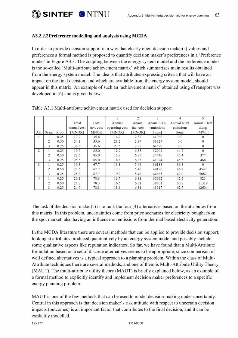
Appendix 3: Multi-criteria decision aid for energy planning 63
A3.2.2.2 Preference modelling and analysis using MCDA In order to provide decision support in a way that clearly elicit decision maker(s) values and preferences a formal method is proposed to quantify decision maker’s preferences in a ‘Preference model’ in Figure A3.3. The coupling between the energy system model and the preference model is the so-called ‘Multi-attribute achievement matrix’ which summarizes main results obtained from the energy system model. The idea is that attributes expressing criteria that will have an impact on the final decision, and which are available from the energy system model, should appear in this matrix. An example of such an ‘achievement matrix’ obtained using eTransport was developed in [6] and is given below.
Table A3.1 Multi-attribute achievement matrix used for decision support.
The task of the decision maker(s) is to rank the four (4) alternatives based on the attributes from this matrix. In this problem, uncertainties come from price scenarios for electricity bought from the spot market, also having an influence on emissions from thermal based electricity generation. In the MCDA literature there are several methods that can be applied to provide decision support, looking at attributes produced quantitatively by an energy system model and possibly include some qualitative aspects like reputation indicators. So far, we have found that a Multi-Attribute formulation based on a set of discrete alternatives seems to be appropriate, since comparison of well defined alternatives is a typical approach to a planning problem. Within the class of Multi-Attribute techniques there are several methods, and one of them is Multi-Attribute Utility Theory (MAUT). The multi-attribute utility theory (MAUT) is briefly explained below, as an example of a formal method to explicitly identify and implement decision maker preferences to a specific energy planning problem. MAUT is one of the few methods that can be used to model decision-making under uncertainty. Central in this approach is that decision maker’s risk attitude with respect to uncertain decision impacts (outcomes) is an important factor that contributes to the final decision, and it can be explicitly modelled. 12X277 TR A6558
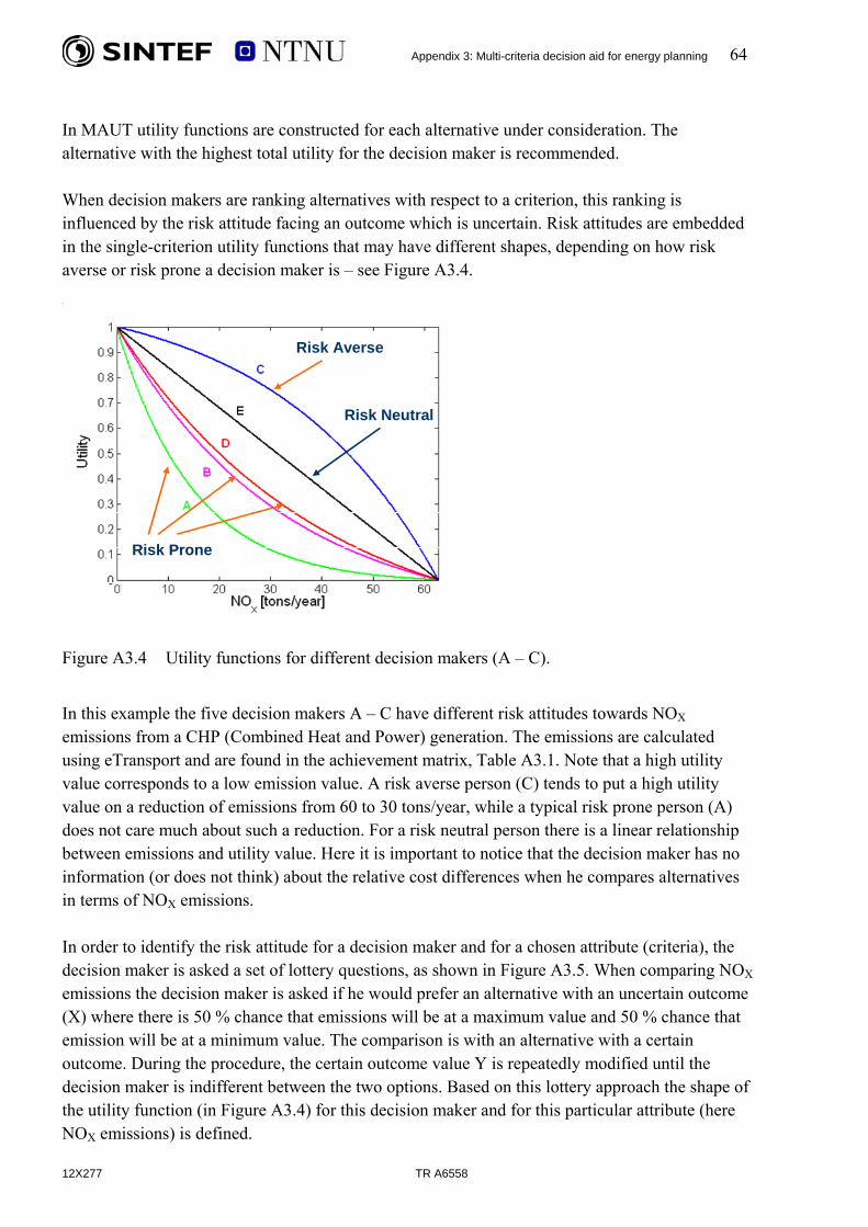
Appendix 3: Multi-criteria decision aid for energy planning 64
In MAUT utility functions are constructed for each alternative under consideration. The alternative with the highest total utility for the decision maker is recommended. When decision makers are ranking alternatives with respect to a criterion, this ranking is influenced by the risk attitude facing an outcome which is uncertain. Risk attitudes are embedded in the single-criterion utility functions that may have different shapes, depending on how risk averse or risk prone a decision maker is – see Figure A3.4.
Risk Averse
Risk Prone
Risk Neutral
Risk Averse
Risk Prone
Risk Neutral
Figure A3.4 Utility functions for different decision makers (A – C).
In this example the five decision makers A – C have different risk attitudes towards NOX emissions from a CHP (Combined Heat and Power) generation. The emissions are calculated using eTransport and are found in the achievement matrix, Table A3.1. Note that a high utility value corresponds to a low emission value. A risk averse person (C) tends to put a high utility value on a reduction of emissions from 60 to 30 tons/year, while a typical risk prone person (A) does not care much about such a reduction. For a risk neutral person there is a linear relationship between emissions and utility value. Here it is important to notice that the decision maker has no information (or does not think) about the relative cost differences when he compares alternatives in terms of NOX emissions. In order to identify the risk attitude for a decision maker and for a chosen attribute (criteria), the decision maker is asked a set of lottery questions, as shown in Figure A3.5. When comparing NOX emissions the decision maker is asked if he would prefer an alternative with an uncertain outcome (X) where there is 50 % chance that emissions will be at a maximum value and 50 % chance that emission will be at a minimum value. The comparison is with an alternative with a certain outcome. During the procedure, the certain outcome value Y is repeatedly modified until the decision maker is indifferent between the two options. Based on this lottery approach the shape of the utility function (in Figure A3.4) for this decision maker and for this particular attribute (here NOX emissions) is defined.
12X277 TR A6558

Appendix 3: Multi-criteria decision aid for energy planning 65
50 %
50 %
X
Y
Uncertain outcome
Certain outcome
Indifference between X and Y
50 %
12X277 TR A6558
32 tonnes/yr100 %
50 %
Uncertain outcome
Certain outcome
Indifference
100 %
0 tonnes/yr
64 tonnes/yr
NOx emissions
50 %
50 %
X
Y
Uncertain outcome
Certain outcome
Indifference between X and Y
50 %
100 %
50 %
Uncertain outcome
Certain outcome
Indifference
45 tonnes/yr32 tonnes/yr
100 %
0 tonnes/yr
64 tonnes/yr
0 tonnes/yr
64 tonnes/yr
NOx emissions
45 tonnes/yr
ui (xi) – individual utility function –
ki – scaling constants –
Figure A3.5 Utility function identification [6].
Attribute preferences (weights)
U (x) – multi-attribute utility function a – alternative with its corresponding set of attributes, ai
i – index corresponding to the set of criteria
( ) ( )1
mi
i ii
U a k u a=
=∑
questionnaire 1
questionnaire 2
[ ]1..i n∈
U (x) – multi-attribute utility function a – alternative with its corresponding set of attributes, ai
i – index corresponding to the set of criteria
ui (xi) – individual utility function –
ki – scaling constants –
( ) ( )1
mi
i ii
U a k u a=
=∑
questionnaire 1
questionnaire 2
[ ]1..i n∈
U (x) – multi-attribute utility function a – alternative with its corresponding set of attributes, ai
i – index corresponding to the set of criteria
ui (xi) – individual utility function –
ki – scaling constants –
( ) ( )1
mi
i ii
U a k u a=
=∑U (x) – multi-attribute utility function a – alternative with its corresponding set of attributes, ai
i – index corresponding to the set of criteria
ui (xi) – individual utility function –
ki – scaling constants –
( ) ( )1
mi
i ii
U a k u a=
=∑
questionnaire 1
questionnaire 2
questionnaire 1
questionnaire 2
[ ]1..i n∈
The utility function for a certain attribute is scaled according to decision maker’s relative preference among criteria [6]. The scaling constants ki (or weights) associated with a certain attribute (criteria) expresses the preference the decision maker gives to this particular attribute compared to the other criteria defined for the problem being analysed. For each decision maker the scaling factors (weights) are identified based on a set of trade-off questions (a second interview round). Attributes are compared pair wise, see Figure A3.6. First, the decision maker has to identify which attribute he considers to be most important. This becomes the reference attribute and is represented on the abscissa axis in Figure A3.6. In this example the reference attribute chosen was the operation cost. Then, two hypothetical alternatives W and Z are considered comparing attribute (i) with the reference (most important) attribute. Alternative W is kept at the best (min) value in the reference attribute (cost) and the worst (max) value in attribute (i), here emissions NOX. Then, alternative Z is kept at the best (min) value in attribute (i) and moved along the reference attribute axis until the decision maker is indifferent to the two alternatives W and Z1. The process is then repeated for the other criteria, comparing each one with the reference criteria.

Appendix 3: Multi-criteria decision aid for energy planning 66
12X277 TR A6558
13 28 Op.cost [Mkr/yr]
64
0
NOX [tonnes/yr]
Z
W Indifference between A and BIndifference between W and Z
Z1 Z0
13 28 Op.cost [Mkr/yr]
64
0
NOX [tonnes/yr]
Z
W Indifference between A and BIndifference between W and Z
Z1 Z0
13 28 Op.cost [Mkr/yr]
64
0
NOX [tonnes/yr]
Z
W
13 28 Op.cost [Mkr/yr]
64
0
NOX [tonnes/yr]
Z
W Indifference between A and BIndifference between W and ZIndifference between A and BIndifference between W and Z
Z0Z0Z1Z1
Figure A3.6 Identification of scaling constants (weights) k by using trade-off questions.
A3.2.3 DERIVING RECOMMENDATIONS The answers of decision makers to all types of preference elicitation questions contributed to the construction of utility functions. In this example expected utilities have been calculated, because several expected electricity price scenarios (with the afferent probabilities) have been considered. The three possible different scenarios in electricity price lead to three possible impact values in all five criteria considered – see Table A3.1. Decision makers have been interviewed with respect to the whole spectrum of possible impacts and the total expected utility functions have been calculated according to the formula:
( )1
p
j j k j k j kk
a p U a=
= ⋅∑ , ,( ) ( )E(Uj(aj)) total expected utility, investment alternative j
Uj,k(xj,k) total utility, alternative j, scenario k
pk probability for scenario k
( )1
p
j j k j k j kk
a p U a=
= ⋅∑ , ,( ) ( )E(Uj(aj)) total expected utility, investment alternative j
Uj,k(xj,k) total utility, alternative j, scenario k
pk probability for scenario k
E UE U
Then, for each decision maker, the four alternatives have been ranked according to the total expected utility. Figure A3.7 shows the results of preference modelling for two decision makers according to expected utility assigned to the alternatives considered. The illustration clearly shows which attributes (criteria) that are considered to be important for a decision maker and why a certain alternative is given a high rank. Note that a high utility value (large “bar”) means that this alternative is preferred (given a high value) by the decision maker.

Appendix 3: Multi-criteria decision aid for energy planning 67
Respondent C
0
0,1
0,2
0,3
0,4
0,5
0,6
0,7
0,8
1 2 3 4
Alternative
Util
ity
Heat dump
12X277 TR A6558
NOxCO2Inv. CostOp. cost
Respondent E
0
0,1
0,2
0,3
0,4
0,5
0,6
0,7
0,8
1 2 3 4
Alternative
Util
ityHeat dumpNOxCO2Inv. CostOp. cost
Local emission (heat dump and NOx) important for decision maker C.
Costs important for decision maker E.
Respondent C
0
0,1
0,2
0,3
0,4
0,5
0,6
0,7
0,8
1 2 3 4
Alternative
Util
ity
Heat dumpNOxCO2Inv. CostOp. cost
Respondent E
0
0,1
0,2
0,3
0,4
0,5
0,6
0,7
0,8
1 2 3 4
Alternative
Util
ityHeat dumpNOxCO2Inv. CostOp. cost
Local emission (heat dump and NOx) important for decision maker C.
Costs important for decision maker E.
Figure A3.7 Synthesis of preference modelling.
A possible approach to improve the interpretation of results form a MAUT analysis is the Equivalent Attribute Technique (EAT) as proposed in [7]. The EAT principle is straightforward. Assume for example that there are two alternatives (a and b) that have different performances in a number of criteria, one of which is cost. An expected total utility has been determined for each alternative, and E(U(a)) > E(U(b)), thus a is preferred to b. For the decision maker this recommendation might not be complete. He/she would probably like to know, for example, how much the cost of the least preferred alternative (b) must be reduced (ΔRed) so that b will reach the same expected utility as a, provided that all other attributes are held at a fix level. ΔRed will be in this case the equivalent cost difference between the two alternatives. Another possibility is to calculate how much the cost of the best alternative a would have to increase (ΔInc) so that its total expected utility will decrease to the value corresponding to alternative b. Figure A3.8 below illustrates this principle for one of the decision makers (DM A) in the example above. For this decision maker, the alternative that gives him the highest utility is alternative 3 (UA, alt3=0,679) while alternative 1 gives him the lowest utility (UA, alt1=0,631). A simplified EAT linear model is used further to determine the equivalent cost reduction (ΔRedA1) that would make the two alternatives equal from the total utility point of view. The figure below shows that the cost for alternative 1 must be reduced from 21,2 MNOK/yr to 20,0 MNOK/yr for this alternative to be assigned the same utility as the original preferred alternative (alternative 3).
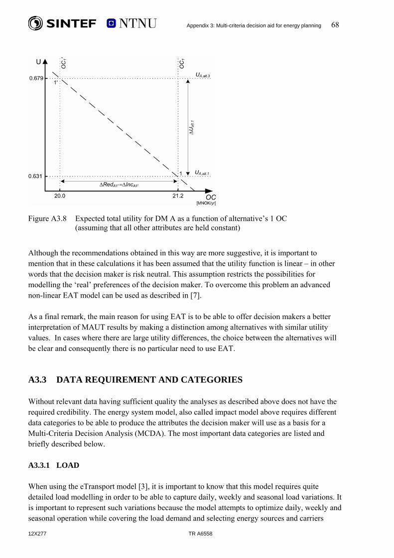
Appendix 3: Multi-criteria decision aid for energy planning 68
Figure A3.8 Expected total utility for DM A as a function of alternative’s 1 OC (assuming that all other attributes are held constant)
Although the recommendations obtained in this way are more suggestive, it is important to mention that in these calculations it has been assumed that the utility function is linear – in other words that the decision maker is risk neutral. This assumption restricts the possibilities for modelling the ‘real’ preferences of the decision maker. To overcome this problem an advanced non-linear EAT model can be used as described in [7]. As a final remark, the main reason for using EAT is to be able to offer decision makers a better interpretation of MAUT results by making a distinction among alternatives with similar utility values. In cases where there are large utility differences, the choice between the alternatives will be clear and consequently there is no particular need to use EAT. A3.3 DATA REQUIREMENT AND CATEGORIES Without relevant data having sufficient quality the analyses as described above does not have the required credibility. The energy system model, also called impact model above requires different data categories to be able to produce the attributes the decision maker will use as a basis for a Multi-Criteria Decision Analysis (MCDA). The most important data categories are listed and briefly described below. A3.3.1 LOAD When using the eTransport model [3], it is important to know that this model requires quite detailed load modelling in order to be able to capture daily, weekly and seasonal load variations. It is important to represent such variations because the model attempts to optimize daily, weekly and seasonal operation while covering the load demand and selecting energy sources and carriers
12X277 TR A6558

Appendix 3: Multi-criteria decision aid for energy planning 69
12X277 TR A6558
according to the optimization criterion. Then, it is also necessary to split load demand into categories. Some load categories are specific to a given energy source or carrier. For example, there are electricity specific load like lighting or supply to other electric appliances. Space heating is a typically flexible type of load that can be covered by alternative sources or carriers (such as gas or district heating). In summary, generating load profiles for the impact model is an important and comprehensive task. In a system analysis load profiles can be built bottom up, starting from end use categories and accumulating to nodes in a network model. From electric power distribution planning there are models and methods available for this task. More details about load and load modelling can be found in Appendix 2. A3.3.2 ENERGY TRANSPORT SYSTEM Energy transport is being modelled in order to capture the geographical dimension, the losses and capacity constraints. Different networks (electric power lines and cables, district heating and gas pipelines) have different physical characteristics. They are mapped into a generic transportation network model with branches and nodes where energy flow, losses and may be voltage or pressure also is modelled. The necessary network data for different energy carriers must be available to accomplish this transport modelling. A3.3.3 GENERATION, CONVERSION AND STORAGE TECHNOLOGIES This type of data encompasses technical descriptions and physical processes from which the attributes associated with energy flow through the transportation network can be developed. In electric power networks these data supports what is usually called load flow or power flow models. For gas networks and district heating networks similar power flow models exist. Therefore, the data needed to model generation, conversion and storage technologies depend closely on the applied network model. Generation and storage technologies are source and carrier specific, while conversion technologies can be carrier specific like AC-DC or DC-AC or they represent conversion from one carrier to another like combined heat and power (CHP). A3.3.4 EMISSIONS Environmental impact from energy processes (generation, conversion, transport and end use) is an important attribute for decision makers. Hence, the physical processes have to be modelled such that the important type of emissions (CO2, NOX, SOX) can be extracted and quantified. A3.3.5 RELIABILITY AND QUALITY Reliability of supply is an important attribute for decision makers. Reliability modelling and analysis is a well known technique for electric power networks. It is then required to have access

Appendix 3: Multi-criteria decision aid for energy planning 70
12X277 TR A6558
to component reliability data bases, and much work has been done to build up such data bases in many countries around the world. In Norway the so-called FASIT computer based system has been established, and this system supports very well reliability analysis of electric power networks. There are also data bases with reliability data for components that belong to other types of equipment, particularly connected to equipment applied in off-shore oil and gas industry. It appears, however, that reliability analysis and associated component data bases are currently not that well established for on-shore gas networks and district heating systems as it is for electric power networks. Regarding quality attributes and indicators for different energy carriers it is well known that voltage quality for electric power is important, and it is currently focused in the Norwegian regulation of electric power supply. Quality indicators that can be used to compare different energy carriers from end user point of view seem currently to be a qualitative and subjective exercise. Then, it seems natural to include this aspect into the preference modelling phase. A3.3.6 COSTS AND PRICES This type of data includes first of all costs and prices connected to equipment used for generation, transport, conversion and end use of energy. There are data bases available, for example for electric power networks there are handbooks such as [10]. Also for other type of equipment costs and prices should be available. Another type of economical data is energy carrier prices that are subject to a market, to transport costs and to taxes. Such data are also available from market operators, network/transport companies and through public channels. For application of such data in system analysis one should remember the principles described in connection with ‘system boundaries’ [9].

Appendix 3: Multi-criteria decision aid for energy planning 71
12X277 TR A6558
A3.4 REFERENCES [1] Løken, E.: Multi-Criteria Planning of Local Energy Systems with Multiple Energy Carriers. Doctoral thesis at NTNU, 2006:62, April 2006. [2] Catrinu, M.D.: Decision Aid for Planning Local Energy Systems. Doctoral thesis at NTNU, 2006:62, April 2006. [3] Bakken, B.H., Wolfgang, O: eTransport, A novel tool for energy planning. Trondheim: SINTEF Energiforskning AS 2006. (TR A6255) [4] Energy Planning Toolbox web-site:
http://www.energy.sintef.no/prosjekt/energyplanningtoolbox/ [5] Catrinu, M., Løken, E., Botterud, A., Holen, A.T.: Constructing a multi-criteria framework
for local energy system planning Proceedings of the 17th International Conference on Multiple Criteria Decision Analysis
(MCDM 2004), Whistler, Canada, August 2004. [6] Botterud, A. ,Catrinu, M., Løken, E., Holen, A.T.: Integrated energy distribution systems
planning: A multi-criteria approach Proceedings of the 15th Power Systems Computation Conference
(PSCC 2005), Liege, Belgium, August 2005. [7] Løken, E., Botterud, A., Holen, A.T.: Use of Equivalent Attribute Technique in Multi-
Criteria Planning of Local Energy Systems. Proceedings of Operational Research Models and Methods in the Energy Sector
(ORMMES’2006), Portugal, September 2006. [8] Matos, Manuel: Tutorial on Application of Risk Analysis and Multi-Criteria Models in
Energy Systems Planning. NTNU, Trondheim, 6-9 October 2003. [9] Sand. K. et al: Planning of mixed energy distribution systems. Part I: Problem definition and principles Trondheim: NTNU/SINTEF Energy Research 2007. (TR A6557) [10] Planleggingsbok for kraftnett
(Handbook for planning of electrical power networks – in Norwegian) Trondheim: SINTEF Energy Research


Appendix 4: Uncertainty 73
12X277 TR A6558
APPENDIX 4: UNCERTAINTY
TABLE OF CONTENTS Page
A4.1 INTRODUCTION .............................................................................................................74
A4.2 CLASSES OF UNCERTAINTIES ...................................................................................74 A4.2.1 EXTERNAL UNCERTAINTIES .......................................................................74 A4.2.2 INTERNAL UNCERTAINTY AND IMPRECISION .......................................74
A4.3 MODELLING UNCERTAINTY ......................................................................................75
A4.4 REFERENCES ..................................................................................................................79
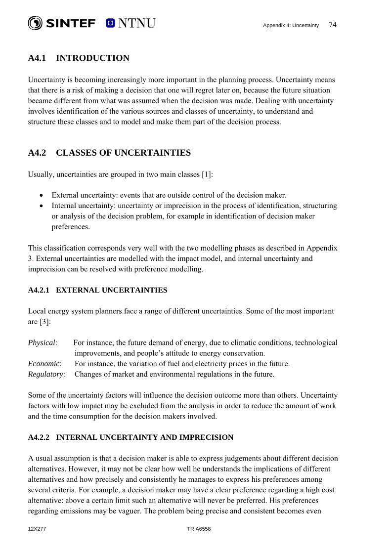
Appendix 4: Uncertainty 74
12X277 TR A6558
A4.1 INTRODUCTION Uncertainty is becoming increasingly more important in the planning process. Uncertainty means that there is a risk of making a decision that one will regret later on, because the future situation became different from what was assumed when the decision was made. Dealing with uncertainty involves identification of the various sources and classes of uncertainty, to understand and structure these classes and to model and make them part of the decision process. A4.2 CLASSES OF UNCERTAINTIES Usually, uncertainties are grouped in two main classes [1]:
• External uncertainty: events that are outside control of the decision maker. • Internal uncertainty: uncertainty or imprecision in the process of identification, structuring
or analysis of the decision problem, for example in identification of decision maker preferences.
This classification corresponds very well with the two modelling phases as described in Appendix 3. External uncertainties are modelled with the impact model, and internal uncertainty and imprecision can be resolved with preference modelling. A4.2.1 EXTERNAL UNCERTAINTIES Local energy system planners face a range of different uncertainties. Some of the most important are [3]: Physical: For instance, the future demand of energy, due to climatic conditions, technological
improvements, and people’s attitude to energy conservation. Economic: For instance, the variation of fuel and electricity prices in the future. Regulatory: Changes of market and environmental regulations in the future. Some of the uncertainty factors will influence the decision outcome more than others. Uncertainty factors with low impact may be excluded from the analysis in order to reduce the amount of work and the time consumption for the decision makers involved. A4.2.2 INTERNAL UNCERTAINTY AND IMPRECISION A usual assumption is that a decision maker is able to express judgements about different decision alternatives. However, it may not be clear how well he understands the implications of different alternatives and how precisely and consistently he manages to express his preferences among several criteria. For example, a decision maker may have a clear preference regarding a high cost alternative: above a certain limit such an alternative will never be preferred. His preferences regarding emissions may be vaguer. The problem being precise and consistent becomes even
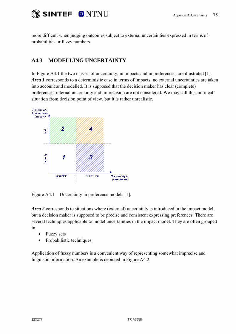
Appendix 4: Uncertainty 75
more difficult when judging outcomes subject to external uncertainties expressed in terms of probabilities or fuzzy numbers. A4.3 MODELLING UNCERTAINTY In Figure A4.1 the two classes of uncertainty, in impacts and in preferences, are illustrated [1]. Area 1 corresponds to a deterministic case in terms of impacts: no external uncertainties are taken into account and modelled. It is supposed that the decision maker has clear (complete) preferences: internal uncertainty and imprecision are not considered. We may call this an ‘ideal’ situation from decision point of view, but it is rather unrealistic.
Figure A4.1 Uncertainty in preference models [1].
Area 2 corresponds to situations where (external) uncertainty is introduced in the impact model, but a decision maker is supposed to be precise and consistent expressing preferences. There are several techniques applicable to model uncertainties in the impact model. They are often grouped in
• Fuzzy sets • Probabilistic techniques
Application of fuzzy numbers is a convenient way of representing somewhat imprecise and linguistic information. An example is depicted in Figure A4.2.
12X277 TR A6558

Appendix 4: Uncertainty 76
50 load
50 load
u(P)
12X277 TR A6558
Figure A4.2 Crisp set (left) and fuzzy set (right) [1], [5]. Figure A4.2 Crisp set (left) and fuzzy set (right) [1], [5].
poss
1
0
poss
1
0 45 55 load 3
poss
1
0 2.7 4 4.4 load
poss
1
0 10 12
“Load about 50 MW” ”Load more or less between 3 and 4 MW”
“Load between 10 and 12 MW”
50 load
poss
1
0 45 55 load 3
poss
1
0 2.7 4 4.4 load
poss
1
0 10 12 50 load
poss
1
0 45 55
poss
1
0 50 load 45 55 load 3
poss
1
0 2.7 4 4.4 load 3
poss
1
0 2.7 4 4.4 load
poss
1
0 10 12 load
poss
1
0 10 12
“Load about 50 MW” ”Load more or less between 3 and 4 MW”
“Load between 10 and 12 MW”
800 P (kW
Figure A4.3 More linguistic (qualitative) expressions and associated possibility functions [5].
In Figure A4.3 one can see the difference between a certain (crisp) value of load and an uncertain (fuzzy) value. The shape of the so-called possibility function corresponds to the linguistic statement as depicted in the same figure. The triangle in the middle is a simpler geometric form than the non linear curve in Figure A4.3, i.e. simpler to handle numerically in fuzzy arithmetic. Another type of techniques classified under Area 2 in Figure A4.1 is the well known probabilistic techniques. Application of probability distributions requires operational experience or measurements that can justify a certain probability distribution function with the associated parameters. Alternatively, subjective probabilities can be applied to model different scenarios. The price scenarios applied in the achievement matrix in Appendix 3, Table A.3.1 is an example of using subjective probabilities. The table depicted in Figure A4.4 is in fact a general form of the achievement matrix where probabilities are associated with the scenarios.
)
1
0
u(P)
800 P (kW)
1
0 770 830
Crisp“A load of 800 kW”
Fuzzy“A load about 800 kW”
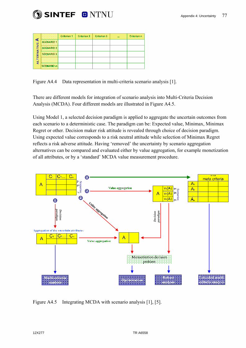
Appendix 4: Uncertainty 77
Figure A4.4 Data representation in multi-criteria scenario analysis [1].
There are different models for integration of scenario analysis into Multi-Criteria Decision Analysis (MCDA). Four different models are illustrated in Figure A4.5. Using Model 1, a selected decision paradigm is applied to aggregate the uncertain outcomes from each scenario to a deterministic case. The paradigm can be: Expected value, Minimax, Minimax Regret or other. Decision maker risk attitude is revealed through choice of decision paradigm. Using expected value corresponds to a risk neutral attitude while selection of Minimax Regret reflects a risk adverse attitude. Having ‘removed’ the uncertainty by scenario aggregation alternatives can be compared and evaluated either by value aggregation, for example monetization of all attributes, or by a ‘standard’ MCDA value measurement procedure.
Scenarios
Decision
paradigm
Utility aggregation
Dec
isio
n pa
radi
gm
Scenarios
Figure A4.5 Integrating MCDA with scenario analysis [1], [5].
12X277 TR A6558

Appendix 4: Uncertainty 78
Model 2 is based on utility theory and tries to capture decision maker risk attitude and attribute preferences into a total utility encompassing all criteria. Probabilities associated with scenarios are handled by application of expected utility. The MAUT method that was described in Appendix 3 is an example of a Model 2 approach. As shown in Figure A3.7, the choice of best alternative is a mono-criterion decision problem looking at expected utility. The two remaining models, 3 and 4 are explained in reference [1]. Area 3 in Figure A4.1 corresponds to the incomplete assessment of certain outcomes. In these cases we are dealing with imprecision in human judgement in situations without external uncertainties. Let us take an example. A decision maker comparing two alternatives in a particular criterion is asked to state if alternative A is preferred to alternative B. Instead of answering ‘yes’ or ‘no’ the answer is like ‘perhaps’, ‘may be’, ‘I do not know’. Particularly if the issue is to state a certain degree of preference (for example in a scale of 1 to 10) the problem of being sure about the answer becomes evident. With application of the method called Analytical Hierarchy Process (AHP) it is allowed to give verbal statements like ‘weakly preferred’ and ‘equally preferred’. The verbal statements are however translated to a numerical scale, and it has been observed that the numerical scale applied may have a decisive impact on the comparison of alternatives. There are methods that allow decision makers to specify interval statements about the elements in a value model. These methods are often classified under so-called preference programming. The consequence of allowing interval statements is that when comparing the overall values for different alternatives one cannot expect a clear recommendation. Most probably we will see overlapping intervals as depicted in Figure A4.6. Then, a final decision paradigm is needed to make the final ranking. This paradigm can be Central value, Maximax, Maximin or Minimax Regret. The essence is: decision maker imprecision is explicitly modelled and a final decision paradigm is applied to resolve this imprecision.
Alt 1
Alt 2
Alt 3
Alt 4
Alt 5
Alt 6
0 0,2 0,4 0,6 0,8 1values
Figure A4.6 Comparing values based on overlapping intervals.
12X277 TR A6558
Appendix 4: Uncertainty 79
12X277 TR A6558
Fuzzy sets can also be applied to translate vague statements into numerical values. Then, fuzzy arithmetic has to be implemented into modelling of decision maker statements. Area 4 in Figure A4.1 corresponds to the incomplete assessment of cases including external uncertainties. Using fuzzy sets is a possible technique to cope with these situations. More explanations can be found in [1]. A4.4 REFERENCES [1] Catrinu, M.D.: Decision Aid for Planning Local Energy Systems. Doctoral thesis at NTNU, 2006:62, April 2006. [2] Botterud, A., Catrinu, M.D., Wolfgang, O., Holen, A.T.: Integrated Energy System
Planning: A Multi-Criteria Approach. Proceedings of the 15th Power Systems Computation Conference, (PSCC2005) Liege,
Belgium, August 2005. [3] Løken, E., Botterud, A., Holen, A.T.: Decision Analysis and Uncertainties in Planning
Local Energy Systems. Proceedings of Probability Methods Applied to Power Systems (PMAPS 2006),
Stockholm, June 2006. [4] Løken, E., Botterud, A., Holen, A.T.: Use of Equivalent Attribute Technique in Multi-
Criteria Planning of Local Energy Systems. Proceedings of Operational Research Models and Methods in the Energy Sector
(ORMMES’2006), Portugal, September 2006. [5] Matos, Manuel: Tutorial on Application of Risk Analysis and Multi-Criteria Models in
Energy Systems Planning. NTNU, Trondheim, 6-9 October 2003.

Appendix 5: Case studies 81
12X277 TR A6558
APPENDIX 5: CASE STUDIES
TABLE OF CONTENTS Page
A5.1 INTRODUCTION .............................................................................................................82
A5.2 CASE-STUDY 1: AN ENERGY COMPANY IS PLANNING NEW ENERGY INFRASTRUCTURE........................................................................................................83 A5.2.1 PROBLEM STRUCTURING .............................................................................83
A5.2.1.1 System boundaries............................................................................83 A5.2.1.2 Identification of alternatives.............................................................84 A5.2.1.3 Identification of criteria ....................................................................85
A5.2.2 MODELLING THE PROBLEM.........................................................................86 A5.2.2.1 Gathering data ..................................................................................86 A5.2.2.2 Considering the uncertainty..............................................................86 A5.2.2.3 Energy system modelling/Impact modelling....................................87 A5.2.2.4 Preference modelling........................................................................88
A5.2.3 USE THE MODELS TO INFORM THE DECISION MAKER.........................89
A5.3 CASE-STUDY 2: ENOVA’S ROLE IN BUILDING NEW ENERGY INFRASTRUCTURE........................................................................................................92 A5.3.1 PROBLEM STRUCTURING .............................................................................93
A5.3.1.1 System boundaries............................................................................93 A5.3.1.2 Identification of alternatives.............................................................93 A5.3.1.3 Identification of criteria ....................................................................93
A5.3.2 MODELLING THE PROBLEM.........................................................................94 A5.3.2.1 Gathering data ..................................................................................94 A5.3.2.2 Considering the uncertainty..............................................................95 A5.3.2.3 Energy system modelling .................................................................95 A5.3.2.4 Preference modelling........................................................................96
A5.3.3 SOME RESULTS FROM ETRANSPORT MODEL .........................................96
A5.4 CASE-STUDY 3: LOAD MODELING............................................................................99 A5.4.1 DESCRIPTION OF PLANNING AREA............................................................99 A5.4.2 SOLUTION PROCEDURE ..............................................................................100 A5.4.3 RESULTS..........................................................................................................101
A5.4.3.1 Design load profiles for heat and electricity demand.....................102 A5.4.3.2 Yearly load profiles and duration profiles......................................103
A5.4.4 CONCLUSION .................................................................................................106
A5.5 REFERENCES ................................................................................................................107

Appendix 5: Case studies 82
12X277 TR A6558
A5.1 INTRODUCTION This appendix presents several case-studies that exemplify the complexity in the process of local energy systems planning. The first two case-studies are examples of energy planning problems, seen from the perspective of different types of decision-makers: an energy distribution company and an authority in charge with supervising and giving incentives for energy infrastructure planning (Enova). These examples will show how decision-makers can use the planning methodology and tools to solve specific planning problems. Each example is structured so that the main challenges for planning (identifying system’s boundaries, alternatives and criteria for analysis) will be first revealed, then the use of different tools to support the final decision will be discussed. The third case-study is about forecasting energy demand. It shows how to use the available tools for load modelling for obtaining important information about the energy demand: maximum loads, yearly energy consumption and load duration profiles. This case study differs from the first two ones because it describes in details only one planning task (energy demand estimation) and not the whole process. However, this task is crucial in planning studies because it provides information that will be used further in the design and the dimensioning of energy distribution infrastructures, with respect to investment (irreversible) and to operation decisions. The case studies presented here are direct applications of the SEDS planning methodology.
Appendix 5: Case studies 83
12X277 TR A6558
A5.2 CASE-STUDY 1: AN ENERGY COMPANY IS PLANNING NEW ENERGY INFRASTRUCTURE
This is an example of a typical planning problem in many regions/towns in Norway. Several local factors – for example the demographic development in some regions – can trigger an expansion/re-enforcement/diversification of the existing local energy distribution system in order to be able to supply the increase in energy demand and/or to connect new customers. The decision maker in this case is the local energy distribution company that is planning to increase the capacity of supply of an existing energy distribution system4. The increase in the local energy demand can be supplied by different energy carriers such as electricity, gas, hot water/district heating or biomass. In this area electricity is the traditional and most common used energy carrier and therefore, the use of a new resource (gas for example) would require that the local energy company will invest in new energy distribution infrastructure (gas and district heating). The material presented here is based on [1-4]. A5.2.1 PROBLEM STRUCTURING A5.2.1.1 System boundaries Primarily, system’s boundaries have been drawn geographically, in order to include the area where an increase in energy demand has been forecasted. The main increase in energy consumption comes from a large area where new residential buildings (over 2000 households) will be constructed in the near future. In addition, a potential for heat demand has been identified at an industrial site. This industry has a large demand of heat (for special industrial processes) that is currently supplied by a local heat generation facility (an oil-fired boiler). However because the boiler is almost reaching optimal life time, and because of increased oil prices, the management of the company is searching for solutions to replace it. One alternative will be to buy the heat from the local distribution company if the costs and other criteria are better that building a new boiler in the backyard. The energy system analysed in this case study consists of the existing electricity distribution system and a new district heating system, provided that the end consumers will be supplied with both electricity and district heating. Gas and electricity are ‘imported’ at system boundary. The electricity import is in terms of quantity of energy imported (with its daily variations) with associated marginal cost (price) at system boundary and emissions. It has been assumed that the electricity import triggers marginal
4 Although the case-study is based on a real planning problem, no reference to company’s name or details about the region will be given here.

Appendix 5: Case studies 84
changes in the global CO2 emissions and that the price of electricity at system border does not include environmental taxes (for CO2 or other local emissions). The gas import is taken into consideration only in terms of quantity and price. This assumption may underestimate the environmental impact from processes outside the selected system boundary. The system analysed can be schematically represented as in Figure A5.1.
gas
New housesCHP
CHP
12X277 TR A6558
electricity
Industrial heat demand
The town
gas
New housesCHP
CHPelectricity
Industrial heat demand
The town
Figure A5.1 A schematic representation of system boundaries.
A5.2.1.2 Identification of alternatives Four investment alternatives have been identified for further investigation. The planning approach to increase the capacity of the local electricity distribution system - in order to be able to accommodate new customers, is compared with the approach of using gas as local energy source and hot water as energy carrier in a new, parallel district heating infrastructure. The first alternative consists of reinforcing the electricity grid with a new supply line to the area, so that one can continue to rely on electricity to supply the local stationary energy demand. A district heating network and a CHP plant is built in the other three alternatives, to serve the heat demand for the customers in the residential area. In addition, a gas boiler is built to meet the peak demand for district heating. In the second alternative, the district heating network also covers the industrial site outside the residential area. The CHP plant is placed at the industrial site, and can also meet the heat demand there, which is currently supplied with a diesel boiler. In alternatives 3 and 4 the CHP plant is placed nearby the residential area. The only difference between these alternatives is the size of the CHP plant. The larger CHP plant in alternative 4 facilitates generation of more electricity, which can be sold to the electricity market when it is profitable to do so. A consequence of higher electricity generation might be excess heat from the CHP plant, which must be dumped to the local surroundings.

Appendix 5: Case studies 85
The following table summarises the four alternatives.
Table A5.1 List of alternatives.
Alternative New el line DH network CHP plant Gas boiler 1 yes no no no 2 no large 3.6 MW 5.0 MW 3 no small 3.6 MW 5.0 MW 4 no small 5.0 MW 5.0 MW
A5.2.1.3 Identification of criteria The main objective for the planner is to cover the increase in energy demand in the area. Within this framework, the planner wants to assure a stable/reliable energy supply, with minimal costs for the consumers and minimal impact on the environment. Therefore, the objectives for this planning problem were organized as following:
Figure A5.2 The hierarchy of objectives.
In this hierarchy one can observe that four of the objectives are related to the system operation planning (operating cost, CO2 emissions, NOX emissions and heat dump from CHP plants to the environment) and one is related to strategic planning (investment cost). In order to deal with the multiple objectives, measurement scales had to be decided for each of these objectives (or criteria):
Table A5.2 Attributes considered in the case-study.
No. Objective Unit 1 Operating cost [MNOK/year] 2 Investment cost [MNOK/year] 3 CO2 emissions [tons/year] 4 NOX emissions [tons/year] 5 Heat dump [MWh/year]
(MNOK is million NOK)
12X277 TR A6558

Appendix 5: Case studies 86
A5.2.2 MODELLING THE PROBLEM A5.2.2.1 Gathering data The data used for this case study was extracted from a realistic case of an existing planning problem in Norway. In order to simplify the analysis we only considered the operations of the system for one time stage (year) in the future. Hence, in this analysis we do not consider the long-term changes in demand, and the timing of investment decisions. Total investment costs were therefore converted to annualised costs and could therefore be compared to the operating costs. An interest rate of 7 % was used for investment costs. Hourly data for electricity and heat demand were specified for 8 different days in the year. The load days represented four seasons and two days within the week (weekday and weekend day). A 122 bus network was used for the electricity grid, with hourly electricity load specified in 55 of them. A simplified load flow model was used to calculate the load flow and the corresponding losses in the impact model. Potential district heating networks were represented with either 14 or 16 heat demand points, all of them with hourly demand data for the 8 load days. Note that while the electricity load can only be met by electricity, any connected energy carrier can meet the heat load. In this case that is electricity or district heating. A5.2.2.2 Considering the uncertainty The main uncertainty considered in the analysis is the price of electricity. The electricity price is very important for the total cost of meeting the load, since there can be substantial exchange of electricity from the area, both imports and exports. Three scenarios were used for hourly prices of electricity, as shown in Figure A5.3. For simplicity the same price data were used for all the 8 load days.
0.001 2 3 4 5 6 7 8 9 10 11 12 13 14 15 16 17 18 19 20 21 22 23 24
Hour
50.00
100.00
150.00
200.00
250.00
300.00
350.00
Pric
e [N
OK
/MW
h]
highbaselow
Figure A5.3 Price scenarios. Currency rate: € 1 ≈ NOK 8.
12X277 TR A6558
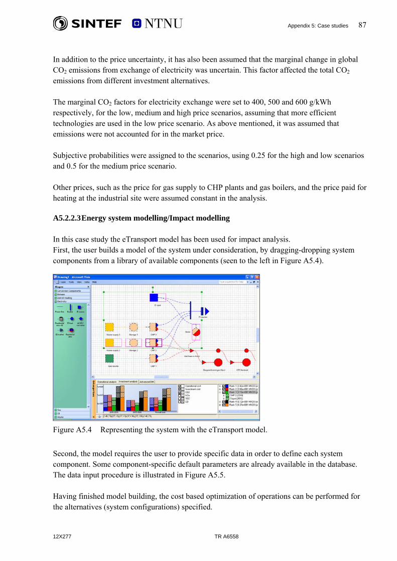
Appendix 5: Case studies 87
In addition to the price uncertainty, it has also been assumed that the marginal change in global CO2 emissions from exchange of electricity was uncertain. This factor affected the total CO2 emissions from different investment alternatives. The marginal CO2 factors for electricity exchange were set to 400, 500 and 600 g/kWh respectively, for the low, medium and high price scenarios, assuming that more efficient technologies are used in the low price scenario. As above mentioned, it was assumed that emissions were not accounted for in the market price. Subjective probabilities were assigned to the scenarios, using 0.25 for the high and low scenarios and 0.5 for the medium price scenario. Other prices, such as the price for gas supply to CHP plants and gas boilers, and the price paid for heating at the industrial site were assumed constant in the analysis. A5.2.2.3 Energy system modelling/Impact modelling In this case study the eTransport model has been used for impact analysis. First, the user builds a model of the system under consideration, by dragging-dropping system components from a library of available components (seen to the left in Figure A5.4).
Figure A5.4 Representing the system with the eTransport model.
Second, the model requires the user to provide specific data in order to define each system component. Some component-specific default parameters are already available in the database. The data input procedure is illustrated in Figure A5.5. Having finished model building, the cost based optimization of operations can be performed for the alternatives (system configurations) specified.
12X277 TR A6558
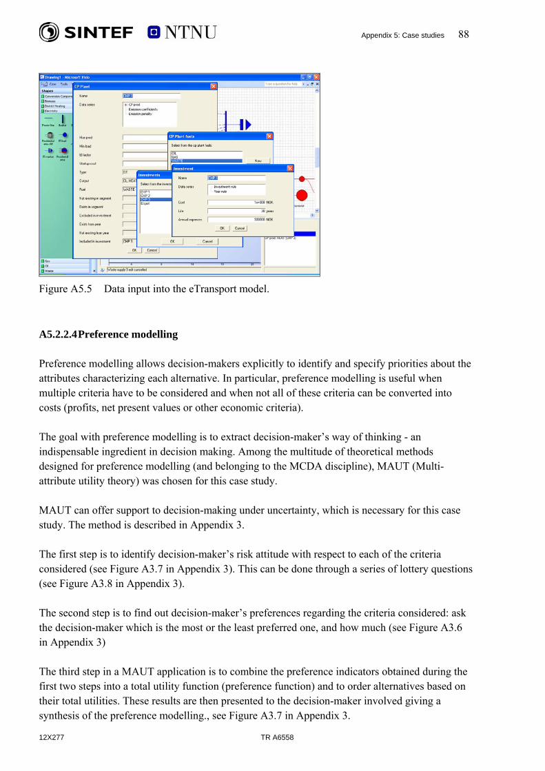
Appendix 5: Case studies 88
Figure A5.5 Data input into the eTransport model.
A5.2.2.4 Preference modelling Preference modelling allows decision-makers explicitly to identify and specify priorities about the attributes characterizing each alternative. In particular, preference modelling is useful when multiple criteria have to be considered and when not all of these criteria can be converted into costs (profits, net present values or other economic criteria). The goal with preference modelling is to extract decision-maker’s way of thinking - an indispensable ingredient in decision making. Among the multitude of theoretical methods designed for preference modelling (and belonging to the MCDA discipline), MAUT (Multi-attribute utility theory) was chosen for this case study. MAUT can offer support to decision-making under uncertainty, which is necessary for this case study. The method is described in Appendix 3. The first step is to identify decision-maker’s risk attitude with respect to each of the criteria considered (see Figure A3.7 in Appendix 3). This can be done through a series of lottery questions (see Figure A3.8 in Appendix 3). The second step is to find out decision-maker’s preferences regarding the criteria considered: ask the decision-maker which is the most or the least preferred one, and how much (see Figure A3.6 in Appendix 3) The third step in a MAUT application is to combine the preference indicators obtained during the first two steps into a total utility function (preference function) and to order alternatives based on their total utilities. These results are then presented to the decision-maker involved giving a synthesis of the preference modelling., see Figure A3.7 in Appendix 3.
12X277 TR A6558

Appendix 5: Case studies 89
A5.2.3 USE THE MODELS TO INFORM THE DECISION MAKER The main tools used for decision support in this case study are an energy system model, also called impact model (eTransport) and a preference model (based on MAUT). The complexity of the analysis is increased by the fact that both economic criteria and criteria describing the environmental impacts (non-monetized) have been considered in the analysis. The use of the two models gives deep insight into the problem. For example, when running the eTransport model, the decision-maker has the opportunity to simulate how the system can be operated in one system configuration (system alternative) during different time-periods and under various price or load scenarios. Figure A5.6 and Figure A5.6 show how the optimization results with this model can be presented to the decision-makers. For example, the model shows the optimal daily operation of each system component or of the system as a whole (Figure A5.6).
Figure A5.6 The operational analysis-mode.
Moreover, the decision-maker can see how investment alternatives are ordered based on their total costs during the period of analysis. The contribution of each cost element (the operating cost, the investment cost or different emission costs) to the total costs figure is also clearly showed (Figure A5.7).
Figure A5.7 The investment analysis mode.
12X277 TR A6558
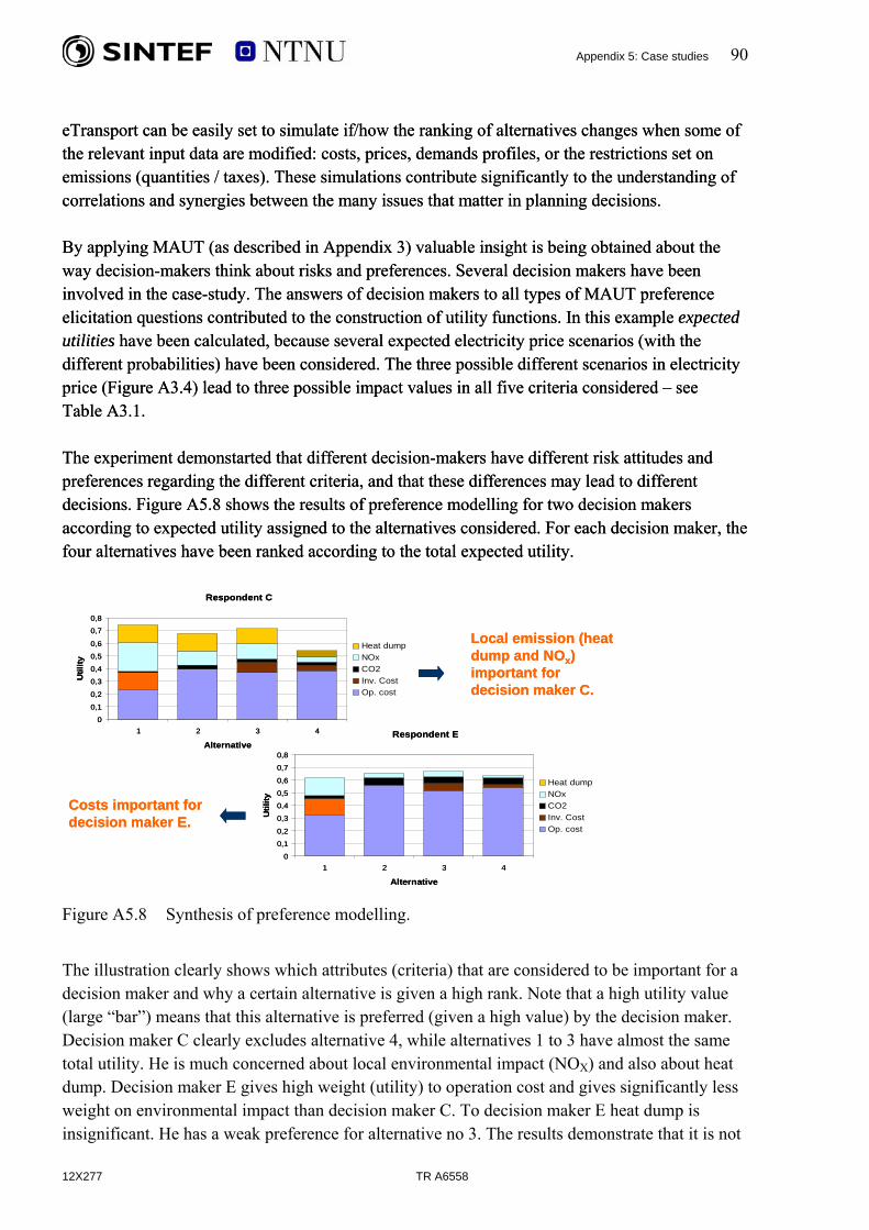
Appendix 5: Case studies 90
eTransport can be easily set to simulate if/how the ranking of alternatives changes when some of the relevant input data are modified: costs, prices, demands profiles, or the restrictions set on emissions (quantities / taxes). These simulations contribute significantly to the understanding of correlations and synergies between the many issues that matter in planning decisions.
eTransport can be easily set to simulate if/how the ranking of alternatives changes when some of the relevant input data are modified: costs, prices, demands profiles, or the restrictions set on emissions (quantities / taxes). These simulations contribute significantly to the understanding of correlations and synergies between the many issues that matter in planning decisions. By applying MAUT (as described in Appendix 3) valuable insight is being obtained about the way decision-makers think about risks and preferences. Several decision makers have been involved in the case-study. The answers of decision makers to all types of MAUT preference elicitation questions contributed to the construction of utility functions. In this example expected utilities have been calculated, because several expected electricity price scenarios (with the different probabilities) have been considered. The three possible different scenarios in electricity price (Figure A3.4) lead to three possible impact values in all five criteria considered – see Table A3.1.
By applying MAUT (as described in Appendix 3) valuable insight is being obtained about the way decision-makers think about risks and preferences. Several decision makers have been involved in the case-study. The answers of decision makers to all types of MAUT preference elicitation questions contributed to the construction of utility functions. In this example expected utilities have been calculated, because several expected electricity price scenarios (with the different probabilities) have been considered. The three possible different scenarios in electricity price (Figure A3.4) lead to three possible impact values in all five criteria considered – see Table A3.1. The experiment demonstarted that different decision-makers have different risk attitudes and preferences regarding the different criteria, and that these differences may lead to different decisions. Figure A5.8 shows the results of preference modelling for two decision makers according to expected utility assigned to the alternatives considered. For each decision maker, the four alternatives have been ranked according to the total expected utility.
The experiment demonstarted that different decision-makers have different risk attitudes and preferences regarding the different criteria, and that these differences may lead to different decisions. Figure A5.8 shows the results of preference modelling for two decision makers according to expected utility assigned to the alternatives considered. For each decision maker, the four alternatives have been ranked according to the total expected utility. Respondent C
0
0,1
0,2
0,3
0,4
0,5
0,6
0,7
0,8
1 2 3 4
Alternative
Util
ity
Heat dumpNOxCO2Inv. CostOp. cost
Respondent E
0,3
0,4
0,5
0,6
0,7
0,8
Util
ity
12X277 TR A6558
0
0,1
0,2
1 2 3 4
Alternative
Heat dumpNOxCO2Inv. CostOp. cost
Local emission (heat dump and NOx) important for decision maker C.
Costs important for decision maker E.
Respondent C
0
0,1
0,2
0,3
0,4
0,5
0,6
0,7
0,8
1 2 3 4
Alternative
Util
ity
Heat dumpNOxCO2Inv. CostOp. cost
Respondent E
0
0,1
0,2
0,3
0,4
0,5
0,6
0,7
0,8
1 2 3 4
Alternative
Util
ity
Heat dumpNOxCO2Inv. CostOp. cost
Local emission (heat dump and NOx) important for decision maker C.
Costs important for decision maker E.
Figure A5.8 Synthesis of preference modelling.
The illustration clearly shows which attributes (criteria) that are considered to be important for a decision maker and why a certain alternative is given a high rank. Note that a high utility value (large “bar”) means that this alternative is preferred (given a high value) by the decision maker. Decision maker C clearly excludes alternative 4, while alternatives 1 to 3 have almost the same total utility. He is much concerned about local environmental impact (NOX) and also about heat dump. Decision maker E gives high weight (utility) to operation cost and gives significantly less weight on environmental impact than decision maker C. To decision maker E heat dump is insignificant. He has a weak preference for alternative no 3. The results demonstrate that it is not
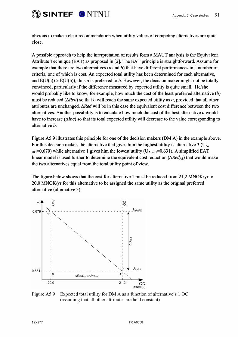
Appendix 5: Case studies 91
obvious to make a clear recommendation when utility values of competing alternatives are quite close. obvious to make a clear recommendation when utility values of competing alternatives are quite close. A possible approach to help the interpretation of results form a MAUT analysis is the Equivalent Attribute Technique (EAT) as proposed in [2]. The EAT principle is straightforward. Assume for example that there are two alternatives (a and b) that have different performances in a number of criteria, one of which is cost. An expected total utility has been determined for each alternative, and E(U(a)) > E(U(b)), thus a is preferred to b. However, the decision maker might not be totally convinced, particularly if the difference measured by expected utility is quite small. He/she would probably like to know, for example, how much the cost of the least preferred alternative (b) must be reduced (ΔRed) so that b will reach the same expected utility as a, provided that all other attributes are unchanged. ΔRed will be in this case the equivalent cost difference between the two alternatives. Another possibility is to calculate how much the cost of the best alternative a would have to increase (ΔInc) so that its total expected utility will decrease to the value corresponding to alternative b.
A possible approach to help the interpretation of results form a MAUT analysis is the Equivalent Attribute Technique (EAT) as proposed in [2]. The EAT principle is straightforward. Assume for example that there are two alternatives (a and b) that have different performances in a number of criteria, one of which is cost. An expected total utility has been determined for each alternative, and E(U(a)) > E(U(b)), thus a is preferred to b. However, the decision maker might not be totally convinced, particularly if the difference measured by expected utility is quite small. He/she would probably like to know, for example, how much the cost of the least preferred alternative (b) must be reduced (ΔRed) so that b will reach the same expected utility as a, provided that all other attributes are unchanged. ΔRed will be in this case the equivalent cost difference between the two alternatives. Another possibility is to calculate how much the cost of the best alternative a would have to increase (ΔInc) so that its total expected utility will decrease to the value corresponding to alternative b. Figure A5.9 illustrates this principle for one of the decision makers (DM A) in the example above. For this decision maker, the alternative that gives him the highest utility is alternative 3 (UA,
alt3=0,679) while alternative 1 gives him the lowest utility (UA, alt1=0,631). A simplified EAT linear model is used further to determine the equivalent cost reduction (ΔRedA1) that would make the two alternatives equal from the total utility point of view.
Figure A5.9 illustrates this principle for one of the decision makers (DM A) in the example above. For this decision maker, the alternative that gives him the highest utility is alternative 3 (UA,
alt3=0,679) while alternative 1 gives him the lowest utility (UA, alt1=0,631). A simplified EAT linear model is used further to determine the equivalent cost reduction (ΔRedA1) that would make the two alternatives equal from the total utility point of view. The figure below shows that the cost for alternative 1 must be reduced from 21,2 MNOK/yr to 20,0 MNOK/yr for this alternative to be assigned the same utility as the original preferred alternative (alternative 3).
The figure below shows that the cost for alternative 1 must be reduced from 21,2 MNOK/yr to 20,0 MNOK/yr for this alternative to be assigned the same utility as the original preferred alternative (alternative 3).
Figure A5.9 Expected total utility for DM A as a function of alternative’s 1 OC
(assuming that all other attributes are held constant)
12X277
TR A6558

Appendix 5: Case studies 92
12X277 TR A6558
The main reason for using EAT is to be able to offer decision makers a better interpretation of MAUT results by making a distinction among alternatives with quite similar utility values. In cases where there are large utility differences, the choice between the alternatives will be clear and consequently there is no particular need to use EAT. This case study demonstrates how decision making including several criteria and several decision makers with different preferences and different risk attitude can be handled by a systematic MCDA method. The decision process becomes transparent, and ranking of alternatives can be explained. A5.3 CASE-STUDY 2: ENOVA’S ROLE IN BUILDING NEW ENERGY
INFRASTRUCTURE The planning concerns the extension of the existing energy distribution system in a town. Unlike the previous example (‘all-electric’) the existing energy distribution system under consideration comprises both the electrical system and a district heating system. The heat is supplied by a district heating plant SARA (Norwegian: Sentrum Avløps Rense Anlegg) that has been used since 1994. This heat plant is composed of two heat pump installations (SARA), two oil boilers and one electric boiler. The material here is based on [5]. The energy balance for the area shows that the maximum forecasted demand is approximately two times larger than the existing capacity of the heat plant. Together with some operation problems these are reasons to seek for upgrading solutions. The possibility of building a new heat plant consisting of a bio-boiler and an oil-boiler, with the associated district heating network is estimated. The decision-maker in this case is Enova which is a governmental agency whose ‘main mission is to contribute to environmentally sound and rational use and production of energy, relying on financial instruments and incentives to stimulate market actors and mechanisms to achieve national energy policy goals’. This agency has the capacity to stimulate energy efficiency by motivating and giving financial support for cost-effective and environmentally sound investment decisions. In relation with this particular case-study, Enova wants to make a decision on what expansion alternative to support financially. However, the existing infrastructure is owned and operated by the local municipality (administration) who is also the main investor in the new infrastructure. In these decision settings, the commune is practically a stakeholder: Enova’s final decision for supporting one of the expansion alternatives will have to be implemented by the commune. Customers that will get access to the district heating network will be also stakeholders in this planning problem. There are no concession rights on the district heating infrastructure. This means that the commune has no obligation to deliver energy or to connect new customers to the

Appendix 5: Case studies 93
12X277 TR A6558
district heating network. Therefore, most of the customers in the area have installed local heat back-ups, small oil-based boilers. This leads to unpredictable loads in the system and consequently to a suboptimal use of the district heating infrastructure. A5.3.1 PROBLEM STRUCTURING A5.3.1.1 System boundaries The ‘target’ area is also defined strictly geographically, as a circle with the centre in the centre of the town and a radius of 2 km. For example, the 22 kV distribution network considered in this study has been cut from the larger local distribution network: only 165 stations (from 732) have been included and those lines that go out from the area (to connect to larger transformer stations) have been defined as electricity-sources at the system border. These supply points have been assigned hourly prices. Electricity price at each customer has been calculated as a sum of an average common price at system border plus the cost of losses in conversion and distribution to each customer location. A5.3.1.2 Identification of alternatives There are two alternatives in this planning problem: to build or not the new heat plant and the afferent district heating network. Initial prospects identified that the best position for the new plant would be in the eastern part of town’s centre and that this plant should have two components - a bio-fuelled boiler (with capacity of 3-4 MW) and an oil-fuelled boiler (with a capacity of 4 MW). It is important to mention that the electricity distribution system does not seem to need major reinforcements in order to cover the possible increase in demand, although the replacement of electricity with other carries in covering the heat demand will alleviate the loading of the electrical network. With the addition of the new heat plant, the local heat supply capacity will increase to 14 GWh/year. However, there is one more condition to include in the analysis. If more than 10 GW heat will be sold annually, concession is obligatory. When concession rights are applied in the region, all new buildings should connect to the district heating networks and therefore be constructed with heating systems based on hot water. A5.3.1.3 Identification of criteria The main objective for the decision-maker in this case-study is to find a candidate for financial support, among the available planning alternatives. As mentioned previously, Enova’s main task is to stimulate energy efficiency by motivating and giving financial support for cost-effective and
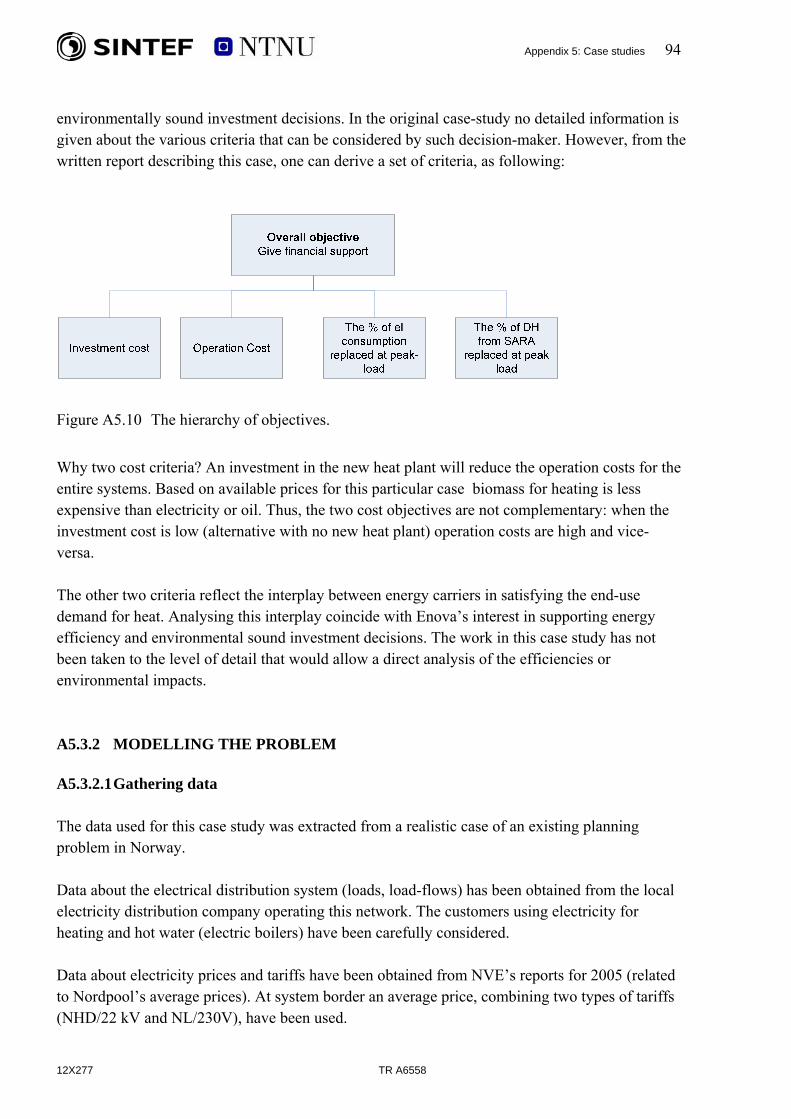
Appendix 5: Case studies 94
environmentally sound investment decisions. In the original case-study no detailed information is given about the various criteria that can be considered by such decision-maker. However, from the written report describing this case, one can derive a set of criteria, as following:
Figure A5.10 The hierarchy of objectives.
Why two cost criteria? An investment in the new heat plant will reduce the operation costs for the entire systems. Based on available prices for this particular case biomass for heating is less expensive than electricity or oil. Thus, the two cost objectives are not complementary: when the investment cost is low (alternative with no new heat plant) operation costs are high and vice-versa. The other two criteria reflect the interplay between energy carriers in satisfying the end-use demand for heat. Analysing this interplay coincide with Enova’s interest in supporting energy efficiency and environmental sound investment decisions. The work in this case study has not been taken to the level of detail that would allow a direct analysis of the efficiencies or environmental impacts. A5.3.2 MODELLING THE PROBLEM A5.3.2.1 Gathering data The data used for this case study was extracted from a realistic case of an existing planning problem in Norway. Data about the electrical distribution system (loads, load-flows) has been obtained from the local electricity distribution company operating this network. The customers using electricity for heating and hot water (electric boilers) have been carefully considered. Data about electricity prices and tariffs have been obtained from NVE’s reports for 2005 (related to Nordpool’s average prices). At system border an average price, combining two types of tariffs (NHD/22 kV and NL/230V), have been used.
12X277 TR A6558

Appendix 5: Case studies 95
12X277 TR A6558
Oil prices at the consumer have been calculated by adding to the oil prices at system border the conversion losses (the efficiency has been set to 0,9 for large boilers and 0,8 for smaller boilers). Oil prices at system border are highly variable, and therefore three price scenarios have been considered in this analysis: 20, 40 and 60 øre/kWh. Several assumptions had to be made about the district heating system. First, the heat source for heat pumps have been considered as a free resource while the costs for electricity used has been calculated as explained above. The price of biomass has been estimated to 14øre/kWh (humid biomass with a burning efficiency of 0,85). Also, the losses in the district heating system have been considered to be 30% for the existing network and 10 % for the new, reinforced network. Loads of potential end-users that are not currently connected to the existing district heating network are also defined, individually. No CO2 taxes have been taken into consideration. It has been assumed that the new investments (alternative 2) will not take place before 2010. Consequently, two periods of analysis have been defined: Period 1 (2005-2010) and Period 2 (2010-2015). Moreover, for each period, it has been assumed a certain increase of demand for electricity and heat. A5.3.2.2 Considering the uncertainty In this case-study the uncertainty in oil price is represented by three price scenarios: 20, 40 and 60 øre/kWh. For biomass it is assumed a price of 14 øre/kWh for humid mass and 17 øre/kWh for dry mass. Then, it is expected that an investment in the bio-boiler might not be profitable without financial support from Enova, depending on the price of biomass. Therefore, the following analysis reveals the maximum biomass price corresponding to a given level of financial support. A5.3.2.3 Energy system modelling The eTransport model is used to model the local energy system. The level of modelling detail is quite high as can be seen from Figure A5.11.

Appendix 5: Case studies 96
Figure A5.11 The model of the local energy system, represented with eTransport.
The model has been used to simulate the operation of the system in each system alternative during different time periods (day, season, year) and to derive the total costs (operation plus investment costs) under each oil price scenario. A5.3.2.4 Preference modelling The scope of this case study was to inform Enova about the energy supply possibilities in the region. Unlike the previous example, the decision-maker has not been involved in the analysis process, and therefore no preference modelling took place. A5.3.3 SOME RESULTS FROM ETRANSPORT MODEL Some results provided by the eTransport model are shown below.The operation of the system without investment in new biomass boiler (left) and with the new investment (right) is found in Figure A5.12. Oil price scenario is 40 øre/kWh.
12X277 TR A6558
Load duration curve 2010-2015
456789
wer
[MW
]
0123
1 31 61 91 121 151 181 211 241 271 301 331 361
Day
Po
OIL NEWOIL SARAOILEL BOILEREL SARABIO NEWHP SARA
Load duration curve 2010-2015
456789
wer
[MW
]
0123
1 31 61 91 121 151 181 211 241 271 301 331 361
Day
Po
OIL NEWOIL SARAOILEL BOILEREL SARABIO NEWHP SARA
Load duration curve 2010-2015
456789
wer
[MW
]
0123
1 31 61 91 121 151 181 211 241 271 301 331 361
Day
Po
OIL NEW
OIL SARAOILEL BOILEREL SARABIO NEW
HP SARA
Load duration curve 2010-2015
456789
wer
[MW
]
0123
1 31 61 91 121 151 181 211 241 271 301 331 361
Day
Po
OIL NEW
OIL SARAOILEL BOILEREL SARABIO NEW
HP SARA
Figure A5.12 Load duration curves: existing system (left) and with new biomass boiler (right).

Appendix 5: Case studies 97
These figures show how the demand is covered during the year and how heat is generated. One can observe that without the expansion of the district heating system (left) peak load demand will be covered by electric boilers and oil. The heat pump (HP SARA) covers most of the base load. If a biomass boiler is introduced, it will replace the (local) electric boilers used as base load. Electric boilers still cover the peak load, now replacing oil. The surprising result, however, is that use of biomass will partly replace another renewable source, the heat pump (SARA). The reason is that the pipeline system connected to the heat pump and the biomass boiler circuit will be physically disconnected due to different water temperatures, and many customers are moved from the heat pump circuit to the biomass boiler circuit if an investment takes place. Energy sources, heating (2010-2015)
10000
15000
20000
25000
Ener
gy[M
Wh/
år]
12X277 TR A6558
0
5000
20 40 60
Oil price [øre/kWh]
EL BOILEROILOIL SARA
EL SARAHP SARA
Energy sources, heating (2010-2015)
10000
15000
20000
25000
Ener
gy[M
Wh/
år]
0
5000
20 40 60
Oil price [øre/kWh]
EL BOILEROILOIL SARA
EL SARAHP SARA
Energy sources, heating (2010-2015)
10000
15000
20000
Ener
gy[M
Wh/
år]
0
5000
20 40 60
Oil price [øre/kWh]
BIO NEWOIL NEWEL BOILEROILOIL SARAEL SARAHP SARA
Energy sources, heating (2010-2015)
10000
15000
20000
Ener
gy[M
Wh/
år]
0
5000
20 40 60
Oil price [øre/kWh]
BIO NEWOIL NEWEL BOILEROILOIL SARAEL SARAHP SARA
Figure A5.13 Sources for covering the heat demand: existing system (left), biomass boiler (right).
The effect of the three different oil price scenarios is depicted in Figure A5.13. For the existing system one can observe that with an oil price of 20 øre/kWh it becomes profitable to use the large-scale oil boiler (SARA) as well as distributed boilers. However, when the oil price is higher, electricity becomes a cheaper energy supply solution. With a new biomass plant the price of oil should be low in order to be profitable to use oil. Biomass replaces oil as well as the heat pump, as explained above. The main question is if it is profitable to make the investment in a new biomass boiler, considering operation costs as well as investment costs. Figure A5. 14 shows the total costs, net present value (NPV) of investment cost + operation cost. With humid biomass the price is 14 øre/kWh, and with dry biomass the price is 17 øre/kWh. The costs have been calculated based on an oil price of 40 øre/kWh.
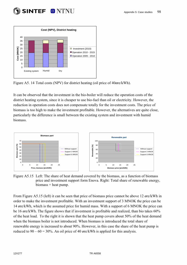
Appendix 5: Case studies 98
Cost (NPV), District heating
0
5
10
1520
25
30
35
40
Humid
Cos
t [M
NO
K]
Investment (2010)
12X277 TR A6558
Operation 2010 - 2015Operation 2005 - 2010
DryExisting system
Cost (NPV), District heating
0
5
10
1520
25
30
35
40
Humid
Cos
t [M
NO
K]
Investment (2010)Operation 2010 - 2015Operation 2005 - 2010
Cost (NPV), District heating
0
5
10
1520
25
30
35
40
Humid
Cos
t [M
NO
K]
Investment (2010)Operation 2010 - 2015Operation 2005 - 2010
DryExisting system
Figure A5. 14 Total costs (NPV) for district heating (oil price of 40øre/kWh).
It can be observed that the investment in the bio-boiler will reduce the operation costs of the district heating system, since it is cheaper to use bio-fuel than oil or electricity. However, the reduction in operation costs does not compensate totally for the investment costs. The price of biomass is too high to make the investment profitable. However, the alternatives are quite close, particularly the difference is small between the existing system and investment with humid biomass. Biomass part
40
50
60
70
spa
rt [%
]
0
10
20
30
0 5 10 15 20 25
Price, biomass [øre/kWh]
Bio
mas
Without supportSupport 3 MNOKSupport 6 MNOK
Biomass part
40
50
60
70
spa
rt [%
]
0
10
20
30
0 5 10 15 20 25
Price, biomass [øre/kWh]
Bio
mas
Without supportSupport 3 MNOKSupport 6 MNOK
0
20
40
0 5 10 15 20 25
Biomass price [øre/kWh]
Ren
ew
60
80
100
able
[%]
Without supportSupport 3 MNOKSupport 6 MNOK
Renewable part
0
20
40
0 5 10 15 20 25
Biomass price [øre/kWh]
Ren
ew
60
80
100
able
[%]
Without supportSupport 3 MNOKSupport 6 MNOK
0
20
40
0 5 10 15 20 25
Biomass price [øre/kWh]
Ren
ew
60
80
100
able
[%]
Without supportSupport 3 MNOKSupport 6 MNOK
Renewable part
Figure A5.15 Left: The share of heat demand covered by the biomass, as a function of biomass
price and investment support form Enova. Right: Total share of renewable energy, biomass + heat pump.
From Figure A5.15 (left) it can be seen that price of biomass price cannot be above 12 øre/kWh in order to make the investment profitable. With an investment support of 3 MNOK the price can be 14 øre/kWh, which is the assumed price for humid mass. With a support of 6 MNOK the price can be 16 øre/kWh. The figure shows that if investment is profitable and realized, than bio takes 60% of the heat load. To the right it is shown that the heat pump covers about 50% of the heat demand when the biomass boiler is not introduced. When biomass is introduced the total share of renewable energy is increased to about 90%. However, in this case the share of the heat pump is reduced to 90 – 60 = 30%. An oil price of 40 øre/kWh is applied for this analysis.

Appendix 5: Case studies 99
12X277 TR A6558
A5.4 CASE-STUDY 3: LOAD MODELING This case study is about forecasting energy demand. It shows how to use the available tools for load modelling (described in Appendix 2) in deriving important information about the energy demand: maximum loads, yearly energy consumption and load duration profiles. This case study differs from the ones presented earlier in this Appendix because it describes in details only one planning task (energy demand estimation) and not the whole process. However, this task is crucial in planning studies because it provides information that will be used further in the design and the dimensioning of energy distribution infrastructures, with respect to investment and operation decisions. The example here shows how generalized load profiles can be applied to a specified planning area in order to estimate the maximum loads, yearly load profiles, load duration profiles and annual energy demands, all divided into heat and electricity purposes. A short description of the planning area along with the solution procedure and results are also presented. This material is based on [6]. A5.4.1 DESCRIPTION OF PLANNING AREA It is important to set the system boundaries when estimating the maximum load and annual energy demand for a planning area. Thus, the following information has to be collected in advance:
• Number of buildings within each building category or archetype. • Available area for each building. • Construction year for each building. • Major retrofitting, if any, for each building. • Type of heating within each building: hydronic heating system or electricity distribution
system only. • Future development, if any, within the system boundaries.
The specified planning area in this example is located in Trondheim, Norway. The case-study is constructed on a fictitious development scenario for this area. This means that all buildings defined within the system boundaries will be built within the planning horizon. Table A5.3 lists the various building categories analyzed in this case-study, and the corresponding average available area. It is assumed that all buildings within the system boundaries will be built within the planning horizon and that all buildings will have hydronic heating systems.
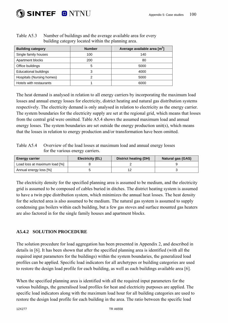
Appendix 5: Case studies 100
12X277 TR A6558
Table A5.3 Number of buildings and the average available area for every building category located within the planning area.
Building category Number Average available area [m2] Single family houses 100 140 Apartment blocks 200 80 Office buildings 5 5000 Educational buildings 3 4000 Hospitals (Nursing homes) 2 5000 Hotels with restaurants 1 6000
The heat demand is analysed in relation to all energy carriers by incorporating the maximum load losses and annual energy losses for electricity, district heating and natural gas distribution systems respectively. The electricity demand is only analysed in relation to electricity as the energy carrier. The system boundaries for the electricity supply are set at the regional grid, which means that losses from the central grid were omitted. Table A5.4 shows the assumed maximum load and annual energy losses. The system boundaries are set outside the energy production unit(s), which means that the losses in relation to energy production and/or transformation have been omitted.
Table A5.4 Overview of the load losses at maximum load and annual energy losses for the various energy carriers.
Energy carrier Electricity (EL) District heating (DH) Natural gas (GAS) Load loss at maximum load [%] 8 2 9 Annual energy loss [%] 5 12 3
The electricity density for the specified planning area is assumed to be medium, and the electricity grid is assumed to be composed of cables buried in ditches. The district heating system is assumed to have a twin pipe distribution system, which minimizes the annual heat losses. The heat density for the selected area is also assumed to be medium. The natural gas system is assumed to supply condensing gas boilers within each building, but a few gas stoves and surface mounted gas heaters are also factored in for the single family houses and apartment blocks. A5.4.2 SOLUTION PROCEDURE The solution procedure for load aggregation has been presented in Appendix 2, and described in details in [6]. It has been shown that after the specified planning area is identified (with all the required input parameters for the buildings) within the system boundaries, the generalized load profiles can be applied. Specific load indicators for all archetypes or building categories are used to restore the design load profile for each building, as well as each buildings available area [6]. When the specified planning area is identified with all the required input parameters for the various buildings, the generalised load profiles for heat and electricity purposes are applied. The specific load indicators along with the maximum load hour for all building categories are used to restore the design load profile for each building in the area. The ratio between the specific load

Appendix 5: Case studies 101
indicator and the relative maximum load for each building is calculated and multiplied by the building’s available area according to the following equation:
Every hour of the weekday’s design load profile is then multiplied by this factor, because the design heat load will always occur during this day type for the buildings analysed. The relative standard deviations for each building are also multiplied by the same factor. The yearly load profiles divided into heat and electricity are calculated based on the generalised load profiles. The HCIs (heat consumption indicators) and ELCIs (electricity consumption indicators) are applied to restore the yearly load profiles for each building within the selected development area using the following equation:
where ECI can be HCI (heat consumption indicator) or ELCI (electricity consumption indicator) depending on purpose, and is measured in [kWh/m2⋅yr]. The design load profiles and yearly load profiles estimated for each building are then aggregated, and the aggregated standard deviation for design load profiles is also found. Details about the aggregation formulas used can be found in [6], chapter 6, paragraph 6.5.1. For this example, the maximum load was estimated using the 95 % t-quantile with n-1 = 310 degrees of freedom, based on the number of buildings within the selected planning area. For this fictitious case study, the tα-value is assumed to be 1.65. The expected yearly load profiles for heat and electricity are estimated based on the DRY for Oslo climate and a reference year respectively see [6]. The HCI and ELCI estimated from the buildings located in Trondheim are applied due to the small difference between the degree days for Trondheim- and Oslo-climate. The load duration profiles are also calculated for both heat and electricity purposes. Finally, the distribution losses for maximum load and annual energy consumption are included in the analysis for each energy carrier. A5.4.3 RESULTS The results in this case-study are in terms of design load profiles divided into heat purposes for every energy carrier and electricity purposes for electricity only. The maximum loads for each scenario are estimated based on the t-quantile analysis. The coincidence factor is given by the design load profiles’ shapes, that is, the maximum load for the area is divided by the sum of the maximum load for each building’s generalised load profile. The yearly load profiles and the load duration profiles for every energy carrier are presented, as well as the expected annual energy demand divided into the different energy carriers.
12X277 TR A6558

Appendix 5: Case studies 102
A5.4.3.1 Design load profiles for heat and electricity demand The load losses have not been differentiated based on the load level throughout the day. The design heat load profiles obtained for the development area are shown in for all energy carriers.
Figure A5.16 Maximum estimated design heat load profiles for all energy
carriers in the planning area analysed.
The maximum load losses are added to the specific load indicators with the percentages tabulated in Table A5.4. One can observe that the maximum heat load will occur at 8 a.m. during weekdays with a heat coincidence factor of 0.975. This is the heat coincidence factor for the generalised load profiles and not the real heat coincidence factor for the development area. The heat load profiles supplied by either electricity or natural gas coincide because the maximum load losses only vary by one per cent. The maximum estimated heat load for the electricity, district heating and natural gas distribution systems are presented in Table A5.5.
Table A5.5 Maximum estimated heat load for the various energy carriers supplying the planning area.
Energy carrier Electricity (EL) District heating (DH) Natural gas (GAS) Maximum heat load 4,70 MWh/h 4,44 MWh/h 4,75 MWh/h
The design electricity load profile for electricity for the development area is shown in Figure A5. 17. The maximum electricity load will occur at 13 p.m. for weekdays with an electricity coincidence factor of 0.899. The maximum electricity load is estimated to 1.54 MWh/h, which constitutes for approximately 25 % of the total load demand for the development area.
12X277 TR A6558

Appendix 5: Case studies 103
Figure A5. 17 Maximum estimated design electricity load profile for the planning area analysed.
The standard deviation is higher for electricity load estimations due to the nature of the electricity load model. The residuals are more scattered when continuous probability distribution analysis rather than regression analysis has been applied. The division of day types is also more challenging for the electricity load model because the climatic influence is diminished by using seasonal load profiles. However, the aggregated standard deviations for both heat and electricity design load profiles decrease relatively as the number of buildings analysed increases. A5.4.3.2 Yearly load profiles and duration profiles The annual heat and electricity losses are added to the HCIs and ELCIs indicators respectively with the percentages tabulated in Table A5.4. The yearly load profiles are shown in Figure A5.18 and Figure A5.19 for heat and electricity demand supplied by district heat and electricity respectively.
Figure A5.18 Yearly and duration heat load profiles for the selected development area.
12X277 TR A6558
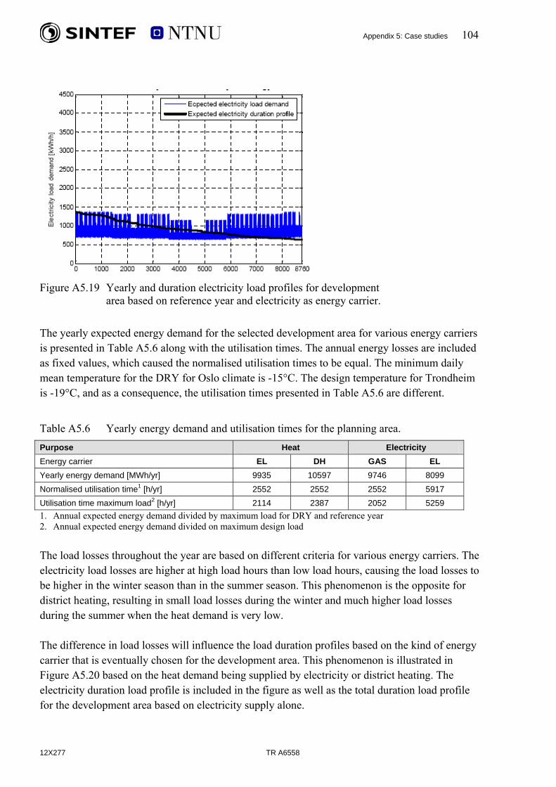
Appendix 5: Case studies 104
Figure A5.19 Yearly and duration electricity load profiles for development
area based on reference year and electricity as energy carrier. The yearly expected energy demand for the selected development area for various energy carriers is presented in Table A5.6 along with the utilisation times. The annual energy losses are included as fixed values, which caused the normalised utilisation times to be equal. The minimum daily mean temperature for the DRY for Oslo climate is -15°C. The design temperature for Trondheim is -19°C, and as a consequence, the utilisation times presented in Table A5.6 are different.
Table A5.6 Yearly energy demand and utilisation times for the planning area. Purpose Heat Electricity Energy carrier EL DH GAS EL Yearly energy demand [MWh/yr] 9935 10597 9746 8099 Normalised utilisation time1 [h/yr] 2552 2552 2552 5917 Utilisation time maximum load2 [h/yr] 2114 2387 2052 5259 1. Annual expected energy demand divided by maximum load for DRY and reference year 2. Annual expected energy demand divided on maximum design load The load losses throughout the year are based on different criteria for various energy carriers. The electricity load losses are higher at high load hours than low load hours, causing the load losses to be higher in the winter season than in the summer season. This phenomenon is the opposite for district heating, resulting in small load losses during the winter and much higher load losses during the summer when the heat demand is very low. The difference in load losses will influence the load duration profiles based on the kind of energy carrier that is eventually chosen for the development area. This phenomenon is illustrated in Figure A5.20 based on the heat demand being supplied by electricity or district heating. The electricity duration load profile is included in the figure as well as the total duration load profile for the development area based on electricity supply alone.
12X277 TR A6558
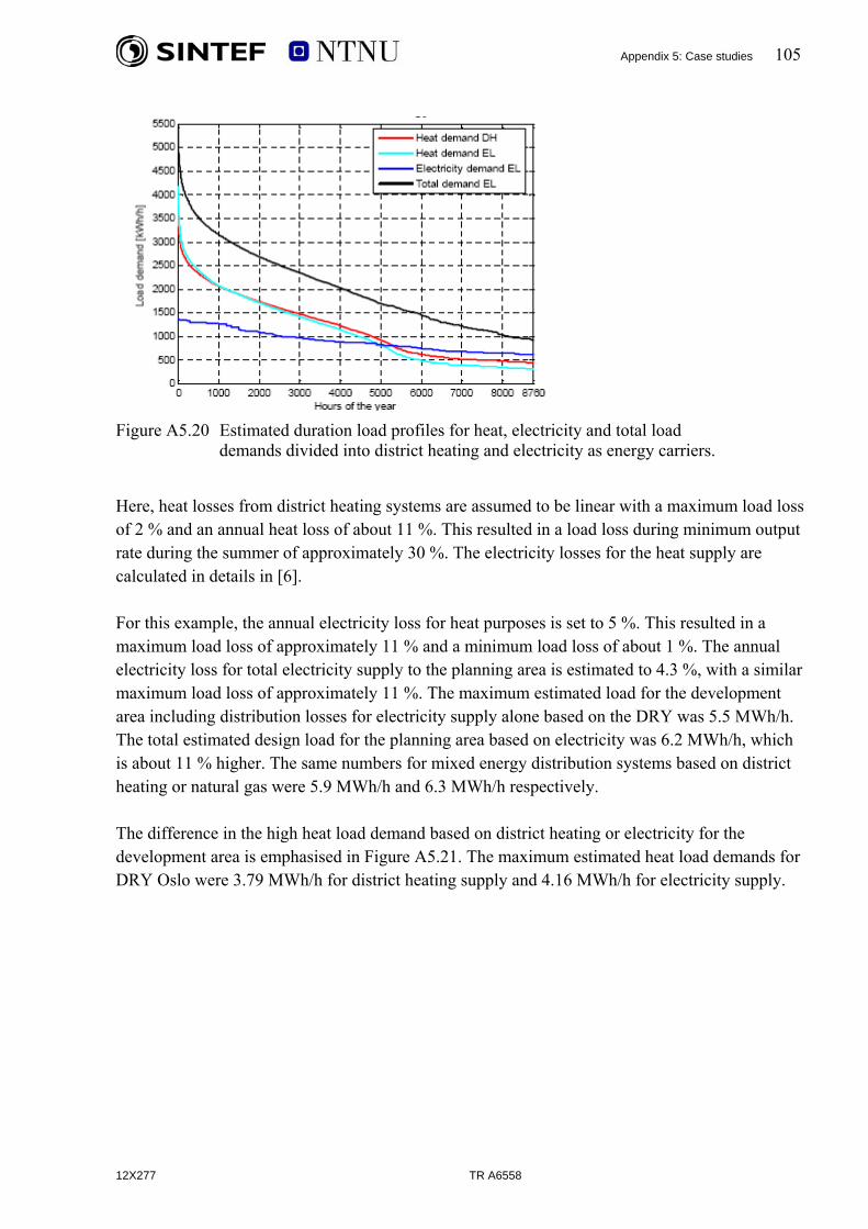
Appendix 5: Case studies 105
Figure A5.20 Estimated duration load profiles for heat, electricity and total load
demands divided into district heating and electricity as energy carriers.
Here, heat losses from district heating systems are assumed to be linear with a maximum load loss of 2 % and an annual heat loss of about 11 %. This resulted in a load loss during minimum output rate during the summer of approximately 30 %. The electricity losses for the heat supply are calculated in details in [6]. For this example, the annual electricity loss for heat purposes is set to 5 %. This resulted in a maximum load loss of approximately 11 % and a minimum load loss of about 1 %. The annual electricity loss for total electricity supply to the planning area is estimated to 4.3 %, with a similar maximum load loss of approximately 11 %. The maximum estimated load for the development area including distribution losses for electricity supply alone based on the DRY was 5.5 MWh/h. The total estimated design load for the planning area based on electricity was 6.2 MWh/h, which is about 11 % higher. The same numbers for mixed energy distribution systems based on district heating or natural gas were 5.9 MWh/h and 6.3 MWh/h respectively. The difference in the high heat load demand based on district heating or electricity for the development area is emphasised in Figure A5.21. The maximum estimated heat load demands for DRY Oslo were 3.79 MWh/h for district heating supply and 4.16 MWh/h for electricity supply.
12X277 TR A6558

Appendix 5: Case studies 106
Figure A5.21 High load segment for the heat load duration profile based on district heating or
electricity as energy carrier.
A5.4.4 CONCLUSION Modelling and forecasting energy demand is an important task in energy planning studies. The doctoral study reported in [6] has provided methods for load modelling of buildings divided into different purposes, such as heat (space heating, ventilation heating and hot tap water) and electricity (lighting, pumps and fans, electrical appliances and others). This case-study has shown how the proposed methods can be applied in practice (although it was a constructed example of a fictitious load development). The reader should also consult reference [6] or Appendix 2 for more details regarding the theoretical background that can support the calculations for this example.
12X277 TR A6558

Appendix 5: Case studies 107
12X277 TR A6558
A5.5 REFERENCES [1] Catrinu, M.D.: Decision Aid for Planning Local Energy Systems. Doctoral thesis at NTNU, 2006:62, April 2006. [2] Løken, E.: Multi-Criteria Planning of Local Energy Systems with Multiple Energy Carriers. Doctoral thesis at NTNU, 2006:62, April 2006. [3] Botterud, A., Catrinu, M.D., Wolfgang, O., Holen, A.T.: Integrated Energy System
Planning: A Multi-Criteria Approach. Proceedings of the 15th Power Systems Computation Conference, (PSCC2005) Liege,
Belgium, August 2005. [4] Løken, E., Botterud, A., Holen, A.T.: Use of Equivalent Attribute Technique in Multi-
Criteria Planning of Local Energy Systems. Proceedings of Operational Research Models and Methods in the Energy Sector
(ORMMES’2006), Portugal, September 2006. [5] Skjelbred, H.I., Wolfgand, O.: Energitransport i Stjørdal. Trondheim: SINTEF Energiforskning AS 2005 (TR A6217) [6] Pedersen L: Load modelling of buildings in mixed energy distribution systems Doctoral thesis at NTNU, 2007:78, February 2007.


SINTEF Energiforskning ASAdresse: 7465 TrondheimTelefon: 73 59 72 00
SINTEF Energy ResearchAddress: NO 7465 TrondheimPhone: + 47 73 59 72 00